





1. Introduction
River systems such as mountain streams or downstream sections of regulated rivers are characterised by coarse-grained beds with gravel or cobbles as the dominant grain sizes due to streamwise grain sorting or limited fine-sediment supply (Ferguson et al. Reference Ferguson, Prestegaard and Ashworth1989; Powell Reference Powell1998). Gravel beds are critical aquatic habitats, providing spawning grounds for fish (Kondolf & Wolman Reference Kondolf and Wolman1993), refugia for macroinvertebrates (Gibbins et al. Reference Gibbins, Vericat, Batalla and Gomez2007) and enabling groundwater–surface water exchange (Pretty & Hildrew Reference Pretty, Hildrew and Trimmer2006). Anthropogenic increases in fine-sediment supply, for example from land-use change or reservoir flushing, can clog the bed surface (Grant Reference Grant, Church, Biron and Roy2012), compromising habitat quality by reducing bed porosity, spawning sites and macroinvertebrate populations (Wharton et al. Reference Wharton, Mohajeri and Righetti2017; Dubuis & De Cesare Reference Dubuis and De Cesare2023). Predicting fine-sediment transport and erosion over coarse substrates is therefore essential for habitat restoration (Grams & Wilcock Reference Grams and Wilcock2007; Kuhnle et al. Reference Kuhnle, Wren and Langendoen2016). However, the processes involved in superficial declogging remain poorly understood (Dubuis & De Cesare Reference Dubuis and De Cesare2023), explanations relying on particle–particle interactions, such as collision-induced entrainment (e.g. Schälchli Reference Schälchli1993). Furthermore, transport models developed for uniform sediment beds (e.g. Meyer-Peter & Müller Reference Meyer-Peter and Müller1948; Smart & Jäggi Reference Smart and Jäggi1983), including those accounting for hiding and exposure effects (e.g. Egiazarov Reference Egiazarov1956; Parker et al. Reference Parker, Klingeman and McLean1982), become unreliable over immobile substrates as they overestimate sediment transport, not accounting for the hydrodynamic impacts of immobile grains (Rickenmann Reference Rickenmann2001; Yager et al. Reference Yager, Kirchner and Dietrich2007; Schneider et al. Reference Schneider, Rickenmann, Turowski, Bunte and Kirchner2015). Crucially, the role of roughness-scale hydrodynamics in interstitial sediment-transport mechanics remains largely unexplored.
Coarse immobile grains protruding from a fine-sediment bed alter the erosion and transport of fine sediments compared with a uniform bed composed of uni-sized sediments (McKenna Neuman & Nickling Reference McKenna Neuman and Nickling1995; Grams & Wilcock Reference Grams and Wilcock2007; Trevisson & Eiff Reference Trevisson and Eiff2022). Two main factors contribute to these alterations: the planar density and protrusion of the immobile grains. In aeolian transport, Al-Awadhi & Willetts (Reference Al-Awadhi and Willetts1999) and Gillies et al. (Reference Gillies, Nickling and King2006) observed a reduction in sediment transport with increasing density due to sediments being trapped in the immobile grains’ lee. This trapping results in an increased critical shear stress for the inception of motion (Gillette & Stockton Reference Gillette and Stockton1989; Iversen et al. Reference Iversen, Wang, Rasmussen, Mikkelsen and Leach1991). Density also affects the amount of sediments available on the surface (Grams & Wilcock 2007, 2014). Indeed, laboratory studies on gravel beds observed that transport scales with the area covered by fine sediments (Yager et al. Reference Yager, Kirchner and Dietrich2007; Kuhnle et al. 2013, 2017). Protrusion further introduces an additional competition: low protrusion tends to enhance transport, whereas high protrusion suppresses it (Nickling & McKenna Neuman Reference Nickling and McKenna Neuman1995; Grams & Wilcock Reference Grams and Wilcock2007; Stradiotti et al. Reference Stradiotti, Righetti, Tarekegn, Wharton and Toffolon2020; Trevisson & Eiff Reference Trevisson and Eiff2022). However, these findings arise from morphodynamic observations alone, and the hydrodynamic mechanisms linking these opposing effects remain largely speculative.
The competition between erosion enhancement and sheltering is expected to depend on the near-bed shear stress, which is highly spatially variable in gravel beds due to the heterogeneity both in immobile-grain and form roughness (Buffin-Bélanger et al. Reference Buffin-Bélanger, Rice, Reid and Lancaster2006; Cooper Reference Cooper2012). Shear stress is governed by coherent structures generated by the roughness elements (e.g. horseshoe vortices) and varies with their protrusion and density, as evidenced by studies on rough beds over immobile substrates composed of hemispheres with varying protrusion (Raus et al. Reference Raus, Moulin and Eiff2019) or of fully exposed boulders with varying density (Fang et al. Reference Fang, Liu and Stoesser2017). The latter studies showed that, for low protrusion or low planar density, the roughness elements behave as isolated obstacles, generating horseshoe vortices with elevated stoss-side shear (e.g. Shamloo et al. Reference Shamloo, Rajaratnam and Katopodis2001; Sutton & McKenna Neuman Reference Sutton and McKenna Neuman2008; Dixen et al. Reference Dixen, Sumer and Fredsoe2013) and lee-side recirculation zones with reduced or even negative shear (Dey et al. Reference Dey, Sarkar, Bose, Tait and Castro-Orgaz2011a ; Hajimirzaie et al. Reference Hajimirzaie, Tsakiris, Buchholz and Papanicolaou2014). On mobile beds, such high- and low-shear regions are thought to produce obstacle marks such as scour holes and sediment shadows (Karcz Reference Karcz1973; Paola et al. Reference Paola, Gust and Southerland1986; Euler et al. Reference Euler, Herget, Schlömer and Benito2017), indicating interaction between flow and morphology.
As protrusion or density increases, the roughness elements no longer act in isolation. Their wakes begin to interact, and the flow transitions to array-like behaviour (Fang et al. Reference Fang, Liu and Stoesser2017; Raus et al. Reference Raus, Moulin and Eiff2019). The classic framework by Morris (Reference Morris1955) identifies three flow regimes for increasing planar density of roughness elements over an immobile, flat bed: isolated, wake-interference and skimming flows. These regimes are characterised by increasing interaction between the wake’s recirculation region and the neighbouring elements until the outer flow is fully disconnected from the interstitial flow. These flow regimes have been predominantly studied under immobile-bed conditions, mainly in relation to their influence on total flow resistance, which peaks at the transition from wake-interference to skimming flow (e.g. Raupach et al. Reference Raupach, Antonia and Rajagopalan1991; Jiménez Reference Jiménez2004; Placidi & Ganapathisubramani Reference Placidi and Ganapathisubramani2015) and decreases at higher densities due to mutual sheltering between roughness elements (Raupach et al. Reference Raupach, Antonia and Rajagopalan1991). Part of the total resistance is expended as form drag on the roughness elements (Marshall Reference Marshall1971; Raupach Reference Raupach1992), reducing the surface shear stress available for fine-sediment transport (Yager et al. Reference Yager, Kirchner and Dietrich2007; Rickenmann & Recking Reference Rickenmann and Recking2011). For example, Canovaro et al. (Reference Canovaro, Paris and Solari2007) observed that, for boulder arrangements maximising the total resistance, less than 40 % contributes to surface shear stress. While such studies provide relevant insights into roughness-induced flow structures and shear partitioning, they are limited by the assumption of an immobile underlying bed, which neglects feedbacks between flow and evolving topography (Neuman & Bédard Reference Neuman and Bédard2015).
Only a few studies investigated the shear stress within the canopy of complex rough beds by varying the protrusion of roughness elements. Smith & Nicholas (Reference Smith and Nicholas2005) and Hardy et al. (Reference Hardy, Best, Lane and Carbonneau2010) investigated the flow over a two-dimensional cast of a gravel bed with varying exposures and over a gravel bed with different sand infilling, respectively, both under fixed bed conditions. In both cases, the lee-side separation region increased with protrusion, suggesting enhanced sheltering. Only recently, Raus et al. (Reference Raus, Moulin and Eiff2019) measured the shear stress on a flat, immobile fine-sediment bed beneath a square array of hemispheres for different protrusion levels
 $P$
(defined as the distance between the hemispheres’ top and the fine-sediment bed divided by the hemisphere’s radius). They found that for
 $P\lt 0.4$
, the shear layer forming at canopy top reaches the immobile fine-sediment bed inducing higher shear stress than a flat uniform sediment bed. For
 $P\gt 0.6$
, the recirculation region fully occupies the interspace, damping the near-bed shear stress. These findings provided the first hydrodynamic evidence based on the local time-averaged shear stress for the competition between erosion enhancement and sheltering, albeit still in the absence of a mobile bed.
In turbulent flows, however, it is the instantaneous turbulent events underlying the time-averaged bed shear stress which set the fine sediments into motion (e.g. Nelson et al. Reference Nelson, McLean and Drake1995; Dwivedi et al. Reference Dwivedi, Melville and Shamseldin2010; Radice et al. Reference Radice, Nikora, Campagnol and Ballio2013). Over uniform beds, transport was shown to depend on the bursting and sweep cycle (Nelson et al. Reference Nelson, McLean and Drake1995; Niño & Garcia Reference Niño and Garcia1996; Sechet & Guennec Reference Sechet and Guennec2000), characterised by a quasi-cyclic alternation of low-speed upward motions, termed ejections, and high-speed inward motions, termed sweeps (Nezu & Nakagawa Reference Nezu and Nakagawa1993). The presence of immobile roughness elements likely modifies these instantaneous events at the fine-sediment level due to roughness-generated coherent motions. Flow investigations at the canopy top observed an increase in the number of sweeps and ejections for increasing density (Papanicolaou et al. Reference Papanicolaou, Diplas, Dancey and Balakrishnan2001) or increasing protrusion of the roughness elements (Smith & Nicholas Reference Smith and Nicholas2005; Wren & Kuhnle Reference Wren and Kuhnle2014). However, within the roughness canopy – in particular near the bed – Raus et al. (Reference Raus, Moulin and Eiff2019) showed that the sweep occurrence decreases with increasing protrusion. This leads to quasi-isotropic turbulence, reducing the near-bed shear stress. Similarly, Fang et al. (Reference Fang, Liu and Stoesser2017) observed that decreasing the spacing between boulders shifts the dominant near-bed turbulent events from sweeps and ejections to inward and outward interactions. These findings suggest that changes in turbulent events within the canopy may influence local sediment transport, yet such changes have not been investigated over mobile beds.
We recently proposed a unifying framework for the morphological and hydrodynamic processes involved in the erosion of fine sediments from rough immobile beds (Trevisson & Eiff Reference Trevisson and Eiff2022). In that study, we investigated the erosion of an initially uniform and mobile fine-sediment bed covering a fixed layer of spheres arranged in a staggered pattern. Single-camera topographic measurements provided time-resolved average bed levels around the spheres as the fine sediments erode. Analysis of the erosion rates revealed four erosive regimes for increasing sphere protrusion with an alternation of erosion-enhancing and erosion-reducing conditions. In the absence of hydrodynamic measurements but based on the evolving planar density as well as angle of attack of the protruding spherical caps inferred from the topographic measurements, the initial decrease in erosion rate for
 $P\lt 0.2$
was attributed to the increased drag exerted by the emerging spheres, named drag-sheltering regime. For higher protrusions (
 $0.2\lt P\lt 0.4$
), the erosion rate increased, consistent with the development of a horseshoe vortex formerly identified for corresponding angles of attack of 20
 $^{\circ}$
–30
 $^{\circ}$
on cones and hemispheres by Okamoto et al. (Reference Okamoto, Yagita and Kataoka1977) and Raus (Reference Raus2019), defining the turbulent enhancement regime. In the third regime (
 $0.4\lt P\lt 0.7$
), named the wake-interference sheltering regime, the erosion rate decreased again as the result of wake-interference flow conditions observed at planar densities
 $0.3 \lt \lambda _p \lt 0.5$
(with
 $\lambda _p$
defined as the ratio of the spheres’ planar area to the total bed area – Grimmond & Oke Reference Grimmond and Oke1999) corresponding to the observed range of
 $P$
. Finally, for
 $P\gt 0.7$
, a skimming-flow sheltering regime with negligible erosion was identified, in agreement with the threshold
 $\lambda _p=0.5$
for skimming-flow conditions (Grimmond & Oke Reference Grimmond and Oke1999). The three transitions in erosive regimes – occurring at given protrusions
 $P$
at least for spheres – were found to be independent of the Shields parameter and the flow depth, suggesting that they are governed purely by geometry. While flow measurements were performed above the spheres, allowing reach-scale morphodynamics (ridges) to be characterised, measurements within the canopy capable of resolving the hydrodynamic processes and the local bed shear stress concurrently with the bed morphology were not possible.
To address this gap, we set up a new measurement configuration for the simultaneous measurement of bed topography, canopy flow and sediment transport. The approach combines a stereo-photogrammetric technique which continuously resolves the evolving bed topography with subgrain-size vertical resolution along with the sediment transport, with a steep-viewing-angle stereo particle image velocimetry (sPIV) technique which captures the interstitial flow within the emerging canopy. The sPIV application is described and validated in Trevisson et al. (Reference Trevisson, Akutina and Eiff2024). The aim is to couple the evolution of the bed morphology with changes in near-bed hydrodynamics for a fine-sediment bed eroding from an immobile bed of spheres, similar to the one analysed by Trevisson & Eiff (Reference Trevisson and Eiff2022).
After presenting the experimental methods, including the statistical definitions of the morphological parameters in § 2, we present the evolution of the bed topography over the entire duration of the experiment (67 hours) at the bedform and pattern scale in § 3. We then analyse the interstitial hydrodynamics at the pattern scale combined with the bed morphology in § 4. The results are discussed in § 5, before drawing conclusions in § 6.
(a) Longitudinal view of the experimental set-up. The green area indicates the measurement area of the sPIV system; (b) staggered pattern of spheres with the reference pattern highlighted in green with
 $l_{x}=4.54$
cm and
 $l_{y}=2.62$
cm. The blue lines indicate the lateral positions of the laser sheet (planes A and B). (c) Cross-sectional view of the sPIV and stereo-photogrammetric systems.

Figure 1. Long description
Panel (a) shows the 9 m recirculating flume. Flow passes through inlet grids, over an 0.8 m ramp and the two-layer bed of spheres, through the measurement section at x = 0 (5.8 m downstream of the inlet), and towards the downstream weir and sediment trap. Ultrasonic sensors monitor water level upstream. At the measurement section, two stereo-PIV cameras and two photogrammetric cameras view the bed through a glass plate at the water surface while a laser illuminates the flow. Panel (b) shows the staggered sphere arrangement. A representative pattern of length l_x = 4.54 cm and width l_y = 2.62 cm is outlined, with laser-sheet planes A at y/l_y = 0 and B at y/l_y = 0.25. Panel (c) shows the cross-sectional optical geometry: the photogrammetric cameras view the bed from above, while the stereo-PIV cameras view the vertical laser sheet at about 70 degrees to the horizontal, enabling flow measurements within the sphere interstices.
2. Experimental methods
2.1. Flume facility
The experiments were conducted in a 9 m long, 30 cm wide and 32 cm high tilting flume at the Institute for Water and Environment at the Karlsruhe Institute of Technology (figure 1
a). Two horizontal and two vertical grids with open areas of 46 % and 64 %, respectively, were installed at the inlet to reduce the turbulence (turbulence intensity
 ${\lt} 2\,\%$
) and uniformise the inflow (spatial variability of the mean streamwise velocity
 ${\lt} 5\,\%$
). The water levels were regulated with a downstream weir and measured with two ultrasonic sensors with a vertical resolution of 0.5 mm and a sampling frequency of 1 Hz. They were positioned 0.35 and 3.9 m upstream of the measuring section to set uniform flow conditions at the beginning of the experiment, as well as to monitor and maintain the water level. The flow rate was measured with a calibrated Venturi meter. A sediment trap installed at the outlet collected the eroded sediments. There was no upstream sediment supply.
2.2. Bed and sediment properties
An immobile gravel bed with mobile sand was modelled similarly to Trevisson & Eiff (Reference Trevisson and Eiff2022) by using immobile polyurethane spheres with a radius
 $R=1$
cm as surrogate gravel, and plastic granulate with a mean diameter
 $d_{50}=1.72$
mm as surrogate sand. The granulate was made of urea, melamine and phenol with a specific weight
 $\rho _{s}=1.49$
 $\mathrm{g\,cm^{-3}}$
and a dry bulk porosity
 $\phi _{s}=0.45$
. It was characterised by a log-normal grain-size distribution like natural sediments. The granulate had a friction angle
 $\phi _f=35^\circ$
(determined with the fixed funnel method), displaying as such a similar frictional behaviour as sand. For a full characterisation of the granulate properties see Trevisson & Eiff (Reference Trevisson and Eiff2022).
Rather than adopting a single layer of spheres as in Trevisson & Eiff (Reference Trevisson and Eiff2022), which is less permeable than a multi-layered bed due to the reduced interstitial-fluid interaction with the surface flow (Manes et al. Reference Manes, Pokrajac, McEvan and Nikora2009), this set-up employed two layers with a combined thickness of 3.3 cm, glued over the entire flume bed (figure 1
a). Thus, a bed matrix with permeability conditions closer to a natural gravel bed was achieved. Each layer was arranged in a staggered symmetric pattern of length
 $l_{x}=4.54$
cm and width
 $l_{y}=2.62$
cm (figure 1
b). The bed’s porosity
 $\phi =0.57$
was comparable to static armoured gravel beds (Aberle Reference Aberle2007). When half-exposed, the spheres of the first layer yielded a planar density
 $\lambda _{p}=S_{p}/S_{r}=0.53$
(with
 $S_{p}$
the spheres’ planar area and
 $S_{r}=l_x l_{y}$
the area of the pattern), characteristic of skimming-flow conditions (Grimmond & Oke Reference Grimmond and Oke1999).
Before the experiment, the spheres were covered with a layer of granulates 4.3 cm thick (i.e. 1 cm above the top of the spheres), to reproduce an immobile gravel bed covered by fine sediments due to a temporary increase in upstream sediment supply. The procedure was as follows: first, the immobile bed was filled with water up to 1 cm over the sphere’s top and the sediments were then poured into the bed matrix to create a fully saturated sediment layer. The bed was then mechanically screeded with a plastic plate to a flat uniform surface to reduce roughness anisotropies. After screeding, the flume was filled with water to reach the desired water level. The flow rate was then carefully increased to the working flow conditions to avoid an abrupt sediment flushing. For this purpose, an 80 cm long ramp inclined by 2.5
 $^\circ$
and covered with glued granulate was installed at the channel entrance with its downstream end 3 mm below the top of the spheres (figure 1
a). In this manner, the shear layer developing at the ramp’s edge breaks up through the presence of the spheres, thereby avoiding a localised erosion with possible downstream influence.
2.3. Flow parameters
A single experiment of 67 hours was performed under uniform flow conditions to investigate the erosive regimes identified by Trevisson & Eiff (Reference Trevisson and Eiff2022). We focus on one experiment since Trevisson & Eiff (Reference Trevisson and Eiff2022) showed that the transitions between erosive regimes depend only on the protrusion level and are independent of the Shields parameter. Yet, due to the more realistic two-layered bed of spheres used here, a lower shear stress (table 1) was applied to reach a similar erosion depth as in experiments 1, 4 and 5 of Trevisson & Eiff (Reference Trevisson and Eiff2022). The difference in shear stress is due to changes in the hyporheic flow in the new bed, which can affect sediment transport (e.g. Rao & Sitaram Reference Rao and Sitaram1999).
Flow parameters of the experiment: water depth
 $H$
, flow rate
 $Q$
, slope
 $i$
, bulk velocity
 $U$
=
 $Q/(WH)$
with
 $W$
the flume width, hydraulic radius with sidewall correction
 $R_{H}$
, bulk shear velocity
 $u_{{*}_b}$
=
 $\sqrt {gR_{H}i}$
, bulk Shields parameter
 $\theta ={u_{{*}_b}^{2}}/({\varDelta g d_{50}})$
, particle Reynolds number
 $Re^{*}$
=
 $u_{{*}_b}d_{50}/\nu$
, bulk Reynolds number
 $Re$
=
 $HU/\nu$
, Froude number
 $Fr$
=
 $U/\sqrt {gH}$
, time duration of the experiment
 $T_{e}$
.

Table 1. Long description
The table lists the uniform-flow conditions used in the 67 h experiment. Water depth H is 5.8 plus or minus 0.05 cm, discharge Q is 4.5 plus or minus 0.5 L/s, and channel slope i is 0.11 plus or minus 0.01 percent. The bulk velocity U is 26 plus or minus 3 cm/s and the side-wall-corrected hydraulic radius R_H is 4.18 plus or minus 0.1 cm. Bulk shear velocity u_*b is 2.3 plus or minus 0.2 cm/s. The bulk Shields parameter theta is 0.065 plus or minus 0.008, approximately twice the critical value used in the study, and the particle Reynolds number Re_* is 40 plus or minus 2. The bulk Reynolds number Re is 15,000 and the Froude number Fr is 0.34. These parameters describe a subcritical, turbulent open-channel flow and provide the constant hydraulic forcing under which the fine-sediment layer erodes, exposing the fixed sphere bed and allowing the successive erosive regimes to develop. The duration covers the evolution to near-static high-protrusion conditions.
The flow parameters are given in table 1. The water depth
 $H$
is defined with reference to the top of the spheres. The bulk shear stress
 $\rho _{f}u_{{*}_b}^2$
acting on the bed was determined from the integral momentum balance for a uniform flow with
 $u_{{*}_b}=\sqrt {gR_{H}i}$
, where
 $i$
is the channel slope,
 $g$
is the gravitational acceleration and
 $R_{H}$
the hydraulic radius with sidewall correction by Chiew & Parker (Reference Chiew and Parker1994). The quantity
 $\rho _{f}u_{{*}_b}^2$
represents the average shear stress acting on a fine-sediment bed located at the top of the spheres. The flow rate was set on the basis of the Darcy–Weissbach equation for a uniform flow, where the friction factor was obtained with the standard logarithmic friction law with an equivalent sand roughness equal to
 $d_{50}$
for uniform sediments (Kironoto & Graf Reference Kironoto and Graf1995; Powell Reference Powell1998).
The sediments were transported as bedload. The bulk Shields parameter
 $\theta =u_{*b}^{2}/(g\varDelta d_{50})$
(with
 $\varDelta =\rho_s/\rho_f -1=0.49$
the submerged relative density of the sediments) was equal to twice the critical Shields parameter
 $\theta _{c}=0.033$
, determined on the basis of the Shields diagram (Shields Reference Shields1936) by means of the explicit relationship by Wu & Wang (Reference Wu and Wang1999).
2.4. Flow development
Flow development was assessed through planar PIV measurements performed at the inlet over the transition between the ramp and the bed of spheres without fine sediments. An outer boundary layer (OBL) develops over the ramp and an internal boundary layer (IBL) over the spheres. The OBL and the IBL are estimated to reach full development 2 m (34
 $H$
) and 3 m (52
 $H$
) downstream of the ramp, respectively. This is consistent with Zampiron et al. (Reference Zampiron, Cameron, Stewart, Marusic and Nikora2023), who measured flow development in uniform rough-bed open channels and concluded that approximately 100
 $H$
from the inlet is required to attain fully developed flow conditions. It is therefore reasonable to assume that uniform fully developed flow conditions are present at the measurement section (100
 $H$
downstream of the inlet, see figure 1
a) under uniform-bed conditions, i.e. at the beginning of the experiment with the flat uniform fine-sediment bed (with just the OBL developing) and at the end, when the spheres uniformly protrude (in the presence of the IBL as well).
When the bed erodes during the experiment, the absence of upstream sediment supply leads to the development of an erosive front which can induce streamwise flow non-uniformities. However, measurements of fine-sediment erosion on a one-layered bed of spheres by Trevisson & Eiff (Reference Trevisson and Eiff2022) performed 3.3 and 5.8 m downstream showed that the erosion dynamics, albeit lagged in time, are similar at both locations, i.e. the erosive regimes are streamwise invariant and unaffected by the erosive front. This suggests that the near-bed flow conditions induced by protruding spheres dominate the morphodynamics over outer-layer flow non-uniformities, in accordance with results showing that the roughness sublayer reaches equilibrium more rapidly than the outer flow in response to streamwise changes in roughness (e.g. Cheng & Castro Reference Cheng and Castro2002; Raus et al. Reference Raus, Moulin and Eiff2019). The near-bed flow can therefore be assumed to locally adjust to the evolving roughness at the measurement location throughout the experiment.
2.5. Measurement configuration
To investigate the bed morphodynamics, simultaneous measurements of the flow field, bed topography and sediment transport were performed at the same location 5.8 m downstream of the inlet (figure 1
a). A sPIV set-up with steep vertical viewing angles was used to measure the flow above and inside the canopy of the protruding spheres down to the fine-sediment bed. The bed topography and the sediment transport were measured with a stereo-photogrammetric system. While the topographic and sediment-transport measurements were performed continuously during the whole experiment, the flow measurements were performed at selected times to investigate specific erosive regimes. The reference system was located at the measurement section on top of the spheres and at the centre of the channel with
 $x$
the streamwise direction,
 $z$
the vertical (figure 1
a) and
 $y$
the lateral (figure 1
c).
2.5.1. Stereo-PIV set-up and processing
The sPIV set-up was developed to measure the canopy flow down to the bed and is described in Trevisson et al. (Reference Trevisson, Akutina and Eiff2024). It consists of a blue (445 nm) continuous laser and of two high-speed cameras looking down through a glass plate with a steep vertical viewing angle (
 $\zeta \approx 70^\circ$
to the horizontal, see figure 1
c). This allows access to the bed interstices down to a maximum erosion depth of
 $z=-2.3R$
(figure 1
c). Laser reflections at the bed are filtered out via in-house fluorescent particles emitting in yellow (570 nm) and a long-pass filter with a cutoff wavelength of 475 nm. The glass plate (hereafter boat) is fixed at
 $z=5.8$
cm, levelled with the undisturbed water surface to avoid optical distortions due to surface waves. As shown in Trevisson et al. (Reference Trevisson, Akutina and Eiff2024), flow perturbations induced by the plate in this configuration are negligible, particularly in the roughness sublayer. During the experiment, slight adjustments of the water surface within
 $\pm 0.5$
mm are performed to keep it in contact with the boat.
Three PIV runs were performed at
 $t\approx [3, 6, 50]$
h, capturing three of the four erosive regimes identified by Trevisson & Eiff (Reference Trevisson and Eiff2022). Due to the fast bed evolution, the first erosive regime could not be captured. During each PIV run, two measurements were performed over the fourth pattern of spheres below the boat (figure 1
a): one in the central plane (A) at
 $y/l_ y=0$
and one in the quarter plane (B) at
 $y/l_ y=0.25$
(blue lines in figure 1(b)), to characterise the hydrodynamic conditions within a representative pattern area,
 $l _x \times l_ y$
(green box in figures 1(b) and 2(a)). The field of view extended from the water surface to the fine-sediment bed over one streamwise pattern length
 $l_x$
(green box in figure 1(a)). The following acronyms will be used: ‘
 $r1, r2, r3$
’ for the three PIV runs and ‘
 $pA$
or
 $pB$
’ for the measurement plane. For
 $r2$
and
 $r3$
, 4500 PIV bursts were recorded during each PIV measurement at a frequency of 5 Hz (equivalent to approximately one bulk time unit
 $H/U$
), low enough to obtain statistically independent samples. The measurement duration of 15 minutes is short enough to consider the fine-sediment bed stationary. However, for
 $r1$
, characterised by a faster evolving bed topography, the measurement duration was reduced to 600 and 500 PIV bursts (acquired also at 5 Hz) over planes A and B, respectively, to guarantee stationary bed conditions. For
 $r2$
and
 $r3$
, convergence errors of the turbulent statistics estimated via the confidence intervals taken with 95 % confidence (Bendat & Piersol Reference Bendat and Piersol2018, p.89) are less than 1 % and 5 % for the first- and second-order moments, respectively. For
 $r1$
, the flow statistics were necessarily not as well converged (2 % and 10 % for the first- and second-order moments for plane A and 3 % and 13 % for plane B).
The images were processed with the Davis PIV software 8.4.0 using an iterative multi-pass algorithm by Wieneke (Reference Wieneke2005). A spatial and a time filter were applied to the data, i.e. the universal outlier detection algorithm by Westerweel & Scarano (Reference Westerweel and Scarano2005) and the multivariate detection algorithm by Griffin et al. (Reference Griffin, Schultz, Holman, Ukeiley and Cattafesta2010), respectively. The final correlation box size was
 $36\times 36$
pixels (
 $2.2\times 2.2$
 $\mathrm{mm^2}$
) with a 50 % overlap. The resulting measurement resolution of approximately 1.7 mm is enough to resolve the Taylor microscale (ranging from 3 to 9 mm) and is comparable to the grain size.
(a) Stereo-PIV measurement region and definition of the protrusion height
 $k(x,y)=$
−
 $z_{b}(x,y)$
; (b) example of a DEM
 $z_{b}$
for
 $t=50.2$
h; (c) two-dimensional field of the protrusion levels of the spheres
 $P=-z_b/R$
obtained from the DEM in (b); (d) lateral profile of the longitudinally averaged protrusion levels
 $\langle P\rangle _{x}$
. The regions contoured in red in (b) and (c) identify the reference pattern of spheres.

Figure 2. Long description
Panel (a) defines the geometry used to quantify sphere protrusion within the stereo-PIV region. The sphere tops define z = 0, the local fine-sediment surface lies below, and protrusion height k is the vertical distance from the sediment surface to the sphere top; protrusion level is P = k/R. Panel (b) shows a digital elevation model at t = 50.2 h, where repeated circular contours identify exposed spheres and colours represent bed elevation. The reference sphere pattern is outlined in red. Panel (c) converts the same bed topography into a two-dimensional protrusion map P = -z_b/R; the exposed spheres appear as holes in the fine-sediment field. Panel (d) shows the longitudinally averaged protrusion profile <P>_x versus lateral position y/W. Values are mostly of order one but vary laterally, reflecting troughs and locally higher sediment levels such as ridges. The profiles and maps provide the morphological variables used throughout the analysis.
2.5.2. Stereo-photogrammetric system
The reconstruction of the bed topography is performed via a stereo-photogrammetric system composed of two iDS high-frequency cameras (model UI-3180 CP Rev. 2.1 with a resolution of
 $2592\times 2048$
pixels) equipped with 50 mm f/1.2 Nikkor lenses. The cameras are installed in the centre of the channel 130 cm above the top of the spheres, symmetrically facing each other at a distance of 85 cm (figure 1
a). The cameras view the measurement area through the boat with a vertical viewing angle of 18
 $^\circ$
, equivalent to the camera stereo angle. A white LED flash lamp is installed above the measurement area to provide uniform lighting.
The measurement area is 28.5 cm wide in the lateral direction to cover the channel width (figure 1(c)) and spans the length of the fourth pattern of spheres beneath the boat (see the longitudinal extension of the digital elevation model (DEM) in figure 2(b)). Each camera captures a burst of nine bed images every 3 minutes with a frequency of 32 Hz throughout the experiment. Only the first image in each burst is used for the bed reconstruction, while the others are used for the sediment-transport measurements (§ 2.5.3). The time resolution is deemed sufficient to resolve the morphological changes of the fine-sediment bed (Trevisson & Eiff Reference Trevisson and Eiff2022).
During the PIV measurements, the photogrammetric system is triggered at a lower frequency of 5 Hz in phase with the sPIV system with a negligible time delay. In this mode, each camera captures a burst of three images. The LED lamp is triggered simultaneously with the photogrammetric cameras to avoid interference with the acquisition of the sPIV images necessitating dark conditions. The stereo-photogrammetric cameras are equipped with long-pass filters with a cutoff wavelength of 590 nm to filter out laser reflections on the bed during the PIV measurements.
The stereo-photogrammetric system is calibrated using the camera pinhole model to represent the optical system mathematically (Luhmann et al. Reference Luhmann, Robson, Kyle and Boehm2014). Internal and external camera parameters are estimated using the calibration method by Zhang (Reference Zhang1999), implemented in the calibration toolbox by Bouguet (Reference Bouguet2010). The calibration is performed underwater to account for optical distortions caused by refraction through the boat and the water surface, as done by Bertin et al. (Reference Bertin, Friedrich, Delmas and Chan2013). A second-order radial and full tangential distortion model (Heikkilä & Silvén Reference Heikkilä and Silvén1997) is applied to correct distortions induced by both lens imperfections and refraction. At the end of the experiment, 30 images of a submerged flat calibration plate (
 $160\times 160\times 1$
mm
 $^{3}$
) with a
 $7\times 7$
dot pattern are captured at various locations and orientations below the boat. Dot detection is performed using a pattern-recognition technique with sub-pixel interpolation (Astruc et al. Reference Astruc, Cazin, Cid, Eiff, Lacaze, Robin, Toublanc and Cáceres2012), achieving a detection accuracy of 0.03–0.05 pixels. Final reprojection errors are below 0.1 pixels.
For the reconstruction of the bed topography, stereo matching of homologous points in the stereo-image pairs of the bed was performed through a pattern-based correlation method exploiting the principles of epipolar geometry and a least-squares image matching technique for sub-pixel interpolation. For each pixel of interest in the downstream camera’s image plane, the corresponding epipolar line in the image plane of the camera upstream is constructed (Ma et al. Reference Ma, Soatto, Kosecka and Shankar Sastry2004). A
 $50\times 50$
pixel reference pattern centred on the target pixel is correlated with a similarly sized search box sliding along the epipolar line. The homologous pixel is identified as the one with the highest correlation value. Due to differing perspective distortions between the cameras, the search-box position and shape are adjusted to minimise the difference in intensity level with the reference pattern via least-squares image matching (Ackermann Reference Ackermann1984). Adjustments include affine transformations for geometric distortions and linear radiometric transformations for intensity corrections. In the presence of protruding spheres lacking surface texture, image matching is restricted to the fine-sediment bed, while spheres are reconstructed analytically. The cloud of fine-sediment bed points is triangulated using projective geometry and re-interpolated to yield a DEM with a regular grid spacing of
 $1\times 1$
 $\mathrm{mm^2}$
within the reference pattern of spheres (figure 1
b) and of
 $3\times 3$
 $\mathrm{mm^2}$
outside. Theoretical estimates of quantisation errors in reconstructed point positions yield
 $\epsilon _x \approx \epsilon _y \approx 70$
 $\mathrm{{\unicode[Arial]{x03BC}} m}$
and
 $\epsilon _z \approx 100$
 $\mathrm{{\unicode[Arial]{x03BC}} m}$
(Benetazzo Reference Benetazzo2006).
2.5.3. Sediment-transport measurements
In the presence of bedload transport, the sediment-transport rate is given by
 $q_{s}=C_{s}v_{s}d_{50}$
(Radice et al. Reference Radice, Malavasi and Ballio2006; Yager & Schmeeckle Reference Yager and Schmeeckle2013), where
 $C_{s}$
is the spatially averaged aerial concentration of displaced grains and
 $v_{s}$
the spatially averaged grain velocity. Since sediment transport is primarily modulated by the sediment concentration and only secondarily by the grain velocity (Lajeunesse et al. Reference Lajeunesse, Malverti and Charru2010),
 $C_{s}$
is used hereafter as a proxy for sediment-transport rates. The concentration
 $C_{s}$
is computed by detecting the number of displaced grains,
 $N_{s}$
, from the subtraction of successive bed images, following a methodology similar to Radice et al. (Reference Radice, Malavasi and Ballio2006), where
 $C_{s}$
is defined as
 \begin{equation} C_{s}=\frac {N_{s}V_{g}}{\Delta x \Delta y d_{50}}, \end{equation}
where
 $V_{g}$
=
 $\pi d_{50}^{3}/6$
is the volume of a grain and
 $\Delta x \Delta y$
the spatial extent of the measurement area. Since
 $N_{s}$
depends on the time lag between image frames, (2.1) provides a concentration averaged both temporally and spatially.
The images obtained from the subtraction of two consecutive frames exhibit zero intensity where no sediment motion occurs and positive or negative values where grains are displaced. Since this subtraction image displays both the initial and final position of the displaced grains, only its positive part is retained. The used plastic granulate, composed of black and white grains in a proportion of 20–80, ensures enough background contrast to distinguish moving particles. Automatic object detection is performed using the method of Otsu (Reference Otsu1979), which binarises the subtraction image into white blobs (representing grains) against a black background. Noise-related small blobs, which do not correspond to actual grain displacements, are filtered out using a morphological erosion filter with a circular structural element of three pixels in diameter (Jähne Reference Jähne2012), followed by a dilation filter of the same size to restore particle dimensions. Following Radice et al. (Reference Radice, Malavasi and Ballio2006), particles smaller than 20 % of the average particle size are excluded. The remaining particles are counted to determine
 $N_{s}$
.
The parameter
 $C_s$
is measured with the camera of the stereo-photogrammetric system positioned downstream of the measurement region. The images are first stereo-rectified and
 $C_s$
is determined within the reference pattern of spheres below the sPIV measurement region (figure 1
b). To capture sediment displacement, a burst of nine images is recorded every 3 minutes, as described earlier. The selected image frequency of 32 Hz ensures a minimum particle displacement of 0.3
 $d_{50}$
between frames. At the same time, the image frequency is high enough to constrain the grain motion to trajectories not overstepping two resting periods of a grain, so that
 $C_{s}$
can be considered instantaneous (Radice et al. Reference Radice, Malavasi and Ballio2006). Each image burst provides eight samples of
 $C_{s}$
, which are averaged to increase measurement accuracy. Comparing
 $N_{s}$
derived from the image processing and from visual counting, the image-processing approach underestimates
 $C_{s}$
by approximately 1 % under conditions of diffuse sediment transport. The measured and observed
 $N_{s}$
tend to converge instead when the spheres protrude and sediment transport tends to zero.
2.6. Morphological parameters
The morphological parameters are defined based on the DEM of the bed topography, describing the two-dimensional field of bed elevation
 $z_{b}(x,y,t)$
within the measurement area, as exemplarily shown in figure 2(b) for
 $t=50.2$
h. The protruding spheres are distinctly identifiable by the circular iso-contour lines. The main morphological parameter is the protrusion level
 $P$
of the spheres,
 $P=k/R$
, where
 $k(x,y)=-z_{b}$
(
 $z_{b} \in \text{fine-sediment bed}$
) is the local protrusion height defined as the distance between the top of the spheres and the local fine-sediment bed level (figure 2
a). Note that
 $P\lt 0$
if the spheres are covered by fine sediments and
 $P\gt 0$
if they are exposed. Figure 2(c) shows an example of a protrusion map obtained from the DEM in figure 2(b). The holes represent the regions where the spheres are protruding.
To analyse the evolution at the bedform scale, the protrusion-level map (as in figure 2(c) for
 $t=50.2$
h) is spatially averaged in the longitudinal direction, yielding a lateral profile of longitudinally averaged protrusion levels
 $\langle P\rangle _{x}$
(y) (see figure 2(d) for a typical lateral profile at
 $t=50.2$
h).
For the analysis of the bed morphodynamics at the pattern scale (i.e. within the reference pattern of spheres outlined in red in figure 2(b)), the following morphological variables are also defined:
-
(i) pattern-averaged protrusion level
 $\langle P\rangle$
, obtained by spatially averaging
$P$
within the reference pattern;
-
(ii) planar density of the spheres
$\lambda _{p}=A_{p}/A_{r}$
, where
$A_{p}$
is the planar area of the protruding spheres and
$A_{r}$
the total planar area of the pattern; -
(iii) erosion rate
$E=(1-\lambda _{p})\textit{CR}\partial _{t}\langle P\rangle$
, where
$C=1-\phi _s$
is the solidity of the fine sediments. The erosion rate
$E$
represents the effective volume of fine sediments eroded from the bed via the
$1-\lambda _p$
term, which accounts for the reduction of area covered by fine sediments once the spheres protrude from the fine-sediment bed (Trevisson & Eiff Reference Trevisson and Eiff2022). This term acts in competition with the enhancement of erosion rates during the second erosive regime, since it reduces the amount of sediments available. Yet, it does not influence the onset and the characteristics of the erosive regimes (Trevisson & Eiff Reference Trevisson and Eiff2022).


3. Morphological evolution at the bedform and pattern scale
The bed evolution is first investigated at the bedform scale to identify bedform structures influencing the local morphology (§ 3.1). In § 3.2, the focus shifts to the pattern scale to quantify the effect of sphere protrusion on erosion and sediment transport and identify erosive regimes. An analysis of the pattern-resolved morphology follows in § 3.3 to assess the impact of the erosive regimes on the local bed topography.
Longitudinally averaged protrusion levels
 $\langle P\rangle _{x}$
as a function of
 $t$
and
 $y$
. The vertical dot-dashed lines represent the time instants of the PIV measurements and the horizontal dashed lines the lateral extent of the reference pattern of spheres.

Figure 3. Long description
The colour map shows longitudinally averaged sphere protrusion <P>_x as a function of elapsed time and lateral position y/W. Red and yellow indicate negative protrusion, when spheres remain buried, whereas green and blue indicate positive protrusion and increasing exposure. During the first approximately 3 h, alternating bands show migrating transverse dunes repeatedly burying and exposing the spheres. A longitudinal ridge with lower protrusion is also visible and migrates laterally. At about 3.23 h, the spheres become permanently exposed across the flume and protrusion rapidly increases towards values of order one in strongly eroded troughs. A less-eroded ridge persists near one side of the channel, broadens and later splits into two branches at about 10.5 h. Horizontal dashed lines delimit the reference pattern; vertical dot-dashed lines mark PIV runs r1 near 3 h, r2 near 6 h and r3 near 50 h.
3.1. Bedform evolution
The bedform evolution is analysed via the longitudinally averaged protrusion level
 $\langle P\rangle _{x}(y,t)$
in figure 3. Since the longitudinal averaging scale (§ 2.6) is much smaller than the wavelength of the developing bedforms,
 $\langle P\rangle _{x}$
preserves their spatial variability and enables their identification. During the first three hours,
 $\langle P\rangle _{x}\lt 0$
(red–yellow regions), indicating that the spheres are fully covered by sediments with initial levels
 $\langle P\rangle _{x}\simeq -1$
. The bed exhibits two-dimensional transverse periodic patterns with crests (red regions with lower
 $\langle P\rangle _x$
) and troughs (yellow regions with higher
 $\langle P\rangle _x$
), corresponding to dunes with an amplitude of approximately 0.5 cm. Despite their small amplitude, these features correspond to dunes rather than ripples, as
 $Re_*\gt 35$
is above the threshold for dune formation (da Silva & Yalin Reference da Silva and Yalin2017). Dunes are indeed expected given the high initial sediment availability (Kleinhans et al. Reference Kleinhans, Wilbers, De Swaaf and Van Den Berg2002). Between 1.1 and 3.23 h, the spheres intermittently emerge (light green patterns of
 $\langle P\rangle _{x}\gt 0$
) but are repeatedly buried by migrating dunes. For
 $t\gt 3.23$
h, the sediment layer above the spheres is fully eroded and the spheres remain permanently exposed across the flume width (light green and blue regions of
 $\langle P\rangle _{x}\gt 0$
).
In terms of lateral topographic variations, a longitudinal band of higher bed elevation (red region of low
 $\langle P\rangle _{x}$
over yellow regions) is observed at
 $y/W\simeq -0.08$
for
 $t\lt 2$
h, indicating the presence of a ridge. This ridge migrates towards the right sidewall near
 $y/W\simeq -0.15$
between
 $t=2$
and
 $t=3$
h (yellow/turquoise region over blue regions). Its coexistence with dunes for
 $t\lt 3.23$
h confirms the superimposition of longitudinal and transverse bedforms, previously reported qualitatively by Trevisson & Eiff (Reference Trevisson and Eiff2022) under similar experimental conditions.
For
 $t\gt 3.23$
h, once the spheres become permanently exposed,
 $\langle P\rangle _{x}$
rapidly increases within about one hour to values of order unity over most of the bed (dark blue regions). These more strongly eroded areas are referred to as troughs (Trevisson & Eiff Reference Trevisson and Eiff2022); there, the bed reaches a stable configuration and only sporadic grain motion is observed visually. The stable configuration is interrupted by a secondary shallow ridge which appears between 4 and 6 h closer to the centre at
 $y/W\simeq -0.025$
, locally perturbing the otherwise homogeneous trough conditions, but disappears shortly thereafter. The main ridge at
 $y/W\simeq -0.15$
is higher (lower protrusion levels) and in contrast to the troughs, it remains morphodynamically active until the end of the experiment, with
 $\langle P\rangle _{x}$
gradually decreasing. For
 $t\gtrsim 6$
h, this ridge begins to enlarge and eventually splits at
 $t\simeq 10.5$
h into a major branch closer to the channel centre and a minor branch closer to the wall. For
 $t\gtrsim 6$
h, erosion is therefore confined to the main ridge, while the troughs remain in static equilibrium. A more detailed analysis of trough and ridge dynamics is provided by Trevisson & Eiff (Reference Trevisson and Eiff2022).
3.2. Pattern-averaged evolution
The local morphodynamics within the reference pattern at the channel centre (between the horizontal dashed lines in figure 3) are investigated in figure 4 via the pattern-averaged protrusion level
 $\langle P \rangle$
, the normalised erosion rate
 $E/E_{P0}$
, and the normalised concentration of displaced sediments
 $C_{s}/C_{\!P0}$
, where
 $E_{P0}$
and
 $C_{\!P0}$
are the erosion rate and sediment concentration for a uniform flat sediment bed, respectively. The experiment to measure
 $E_{P0}$
and
 $C_{\!P0}$
is detailed in Appendix A. To obtain robust erosion rates (§ 2.6) and avoid spurious gradients,
 $\langle P \rangle$
is smoothed using a smoothing spline (blue dashed line in figure 4(a)). For clarity, the results in figure 4 are plotted for
 $t\gt 0.8$
h only.
As seen in figure 3, dunes dominate the early stage (
 $t\lt 3.23$
h), during which
 $\langle P \rangle$
,
 $E/E_{P0}$
and
 $C_{s}/C_{\!P0}$
oscillate due to the dunes’ passage in figure 4(a–c). Local minima in
 $\langle P \rangle$
correspond to dune crests and maxima to dune tails, with peaks in displaced sediments occurring over the crests and erosion peaks over the tails consistent with flow acceleration on the dunes’ stoss (Best Reference Best2005; Sarkar & Dey Reference Sarkar and Dey2020).
Once the spheres become permanently exposed at
 $t\simeq 3.23$
h,
 $\langle P \rangle$
increases rapidly within 20 minutes to approximately
 $0.8$
(inset in figure 4(a)). The slight subsequent decrease in
 $\langle P \rangle$
(i.e. sediment deposition) is due to the development of the secondary ridge close to the centre around
 $t \simeq 4$
h (figure 3), followed by a renewed increase from
 $t \simeq 4.5$
h as the ridge is progressively eroded. Nevertheless, as shown by Trevisson & Eiff (Reference Trevisson and Eiff2022), the same erosive trends are observed over ridges and troughs, indicating that the secondary ridge does not affect the dynamics of the erosive regimes. For
 $t\gtrsim 6$
h, the influence of the secondary ridge becomes negligible and
 $\langle P \rangle$
gradually increases, stabilising around unity by
 $t\simeq 11$
h. The oscillations observed thereafter fall within the vertical measurement accuracy (
 $\pm$
0.1 mm), indicating a stable bed.
Temporal evolution of the pattern-averaged protrusion level
 $\langle P\rangle$
(a), of the erosion rates
 $E$
(b) and of the concentration of displaced sediments
 $C_{s}$
(c). The quantities
 $E$
and
 $C_{s}$
are normalised by the erosion rates and the concentration of displaced sediments for a uniform fine-sediment bed,
 $E_{P0}$
and
 $C_{\!P0}$
, respectively. The blue line in (a) represents the smoothed
 $\langle P\rangle$
profile to estimate the erosion rates. The vertical lines identify the time at which the spheres protrude without being covered again (continuous) and the time of the first (dashed), second (dot-dashed) and third (dotted) transition in erosive behaviour. The green dots in (a) identify the PIV runs.

Figure 4. Long description
Panel (a) shows pattern-averaged protrusion <P>. Before about 3.23 h it oscillates as dunes pass; after permanent sphere exposure, it rises rapidly to about 0.8 and later approaches one. The inset identifies critical protrusions near 0.15, 0.43 and 0.8 separating the four erosive regime; green markers show the PIV runs. Panel (b) shows erosion rate E normalized by the uniform-bed value E_P0. After exposure, erosion first falls below half the reference value, rises again to a local maximum just below E_P0, then decreases through ER3 and becomes negligible in ER4 after about 9 h. Panel (c) shows displaced-sediment concentration C_s/C_P0. It follows a similar but slightly delayed sequence: after a local minimum, it peaks near 1.4 times the uniform-bed value at about 3.57 h and then progressively declines. Low, intermittent particle motion remains in ER4 despite negligible net erosion. Vertical lines mark permanent exposure and the three regime transitions.
The normalised erosion rate
 $E/E_{P0}$
in figure 4(b) shows a peak just before the spheres become permanently exposed at
 $t=3.23$
h, caused by the last dune’s passage. For
 $t\geq 3.23$
h,
 $E$
decreases below
 $E_{P0}$
(inset in figure 4(b)), reaching a first local minimum at
 $t=3.36$
h (vertical dashed line) where the erosion rate drops below 50 % of the uniform-bed value. Subsequently,
 $E$
increases again, attaining a local maximum slightly lower than
 $E_{P0}$
at
 $t=3.52$
h (vertical dot-dashed line), before decreasing and becoming negligible for
 $t\gt 9$
h.
The temporal evolution of
 $E/E_{P0}$
can be divided into four erosive regimes for
 $t\gt 3.23$
h when
 $\langle P \rangle \gt 0$
(inset in figure 4(a)). The first erosive regime (ER1: blue shading in figure 4(a–c)) is characterised by a rapid decrease in erosion rates, the second one (ER2: red shading) by an increase, the third one (ER3: green shading) by a further decrease (not necessarily monotonic) and the fourth one (ER4: yellow shading) by a negligible erosion rate. These regimes are consistent with those identified by Trevisson & Eiff (Reference Trevisson and Eiff2022). The transitions are defined by the first local minimum in
 $E/E_{P0}$
(ER1
 $\rightarrow$
ER2), the subsequent by a local maximum (ER2
 $\rightarrow$
ER3) and the last at the time beyond which
 $E$
no longer exceeds
 $0.5\,\%$
of
 $E_{P0}$
at any later time (ER3
 $\rightarrow$
ER4). The corresponding transition times are indicated by dashed, dot-dashed and dotted vertical lines in figure 4(a–c). These transitions occur at critical protrusion levels
 $\langle P_{c1}\rangle =0.15$
,
 $\langle P_{c2}\rangle =0.43$
and
 $\langle P_{c3}\rangle =0.8$
, consistent with Trevisson & Eiff (Reference Trevisson and Eiff2022). The measured planar densities at the second and third transitions,
 $\lambda _{p,c2}=0.34$
and
 $\lambda _{p,c3}=0.49$
, suggest a transition from isolated to wake-interference flow and from wake-interference to skimming flow (Grimmond & Oke Reference Grimmond and Oke1999), respectively.
The normalised sediment-transport rate
 $C_{s}/C_{\!P0}$
(figure 4
c) follows a similar overall evolution. After the sphere exposure at t
 $\simeq$
3.23 h,
 $C_{s}/C_{\!P0}$
exhibits a peak followed by a local minimum at
 $t\simeq 3.46$
h and a subsequent maximum at
 $t=3.57$
h which exceeds sediment-transport rates over a uniform bed by 40 % (inset in figure 4(c)). Thereafter,
 $C_s$
has a decreasing trend until the end of the experiment suggesting that sediment transport will eventually cease. The low transport rates in ER4 up to 30 % of
 $C_{\!P0}$
indicate still an active surface. However, visual observations show that in ER4 particles undergo short, intermittent displacements being rapidly redeposited nearby or trapped in sediment shadows, resulting in a negligible net longitudinal flux consistent with the negligible erosion rates in figure 4(b).
While
 $C_s$
generally follows the same trend as
 $E$
, the
 $C_s$
-extrema are slightly delayed (compare the insets in figures 4(b) and 4(c)). This lag probably reflects a longer adjustment time of sediment transport to the changing flow conditions. Since the erosion rates correspond to the longitudinal variation in sediment-transport rates (Trevisson & Eiff Reference Trevisson and Eiff2022), a lag between the erosion and sediment-transport extrema is possible.
3.3. Pattern-resolved evolution
The spatial organisation of the erosive regimes at the pattern scale is illustrated in figure 5, which shows the evolution of the bed elevation
 $z_b/R$
along the pattern centre (
 $y/W=0$
) at selected times during the four erosive regimes. During ER1 (
 $3.23 \lt t \leq 3.37$
h), the bed remains nearly uniform, with similar levels in the sphere’s lee, stoss and centre, resulting in an essentially horizontal profile. In ER2 (
 $3.37 \lt t \leq 3.52$
h), a pronounced heterogeneity develops: higher bed levels in the sphere’s lee, lower at the centre and intermediate on the stoss side indicate the formation of a sediment shadow for
 $x/l_x \lt 0.45$
. This sediment redistribution resembles that observed during horseshoe vortex development around isolated obstacles (Dixen et al. Reference Dixen, Sumer and Fredsoe2013; Euler et al. Reference Euler, Herget, Schlömer and Benito2017). The slight depression at the pattern centre is attributed to flow acceleration between the central spheres, which act as a contraction (see § 4.2).
Longitudinal profiles of bed elevations
 $z_{b}$
at y/
 $W$
= 0 at selected times during the four erosive regimes.

Figure 5. Long description
The graph shows longitudinal fine-sediment bed profiles z_b/R along the centre of one sphere pattern, from the upstream sphere at x/l_x = 0 to the downstream sphere at x/l_x = 1, at selected times from 3.23 to 60 h. In ER1 the bed remains comparatively flat, indicating similar elevations in the sphere lee, pattern centre and downstream stoss. In ER2 a clear spatial asymmetry develops: sediment remains higher in the upstream sphere’s lee, the bed is lower towards the centre, and intermediate to lower near the downstream stoss, forming a sediment shadow in the lee. Through ER3 this shape persists while the overall bed level shifts downward as erosion continues. In ER4 the profiles approach their lowest, nearly stable elevations. The lee-side sediment shadow remains visible up to about 20 h, after which lee, centre and stoss elevations converge, although localized fluctuations persist because of intermittent deposition and erosion.
In ER3 (
 $3.52\lt t\leq 9$
h), this spatial structure persists, with sediment trapping in the sphere’s lee, while the overall bed levels shift downward. In ER4 (
 $t\gt 9$
h), the sediment shadow remains visible up to
 $t=20$
h, after which the bed levels in the lee converge with those in the central and stoss regions. However, bed-level fluctuations remain larger in the lee, reflecting intermittent deposition and erosion.
Overall, as long as
 $C_s/C_{\!P0}\gt 0.3$
, sediment shadows are continuously replenished by newly transported grains that are temporarily deposited. As transport becomes increasingly intermittent in ER4, sediment supply diminishes and the shadow gradually weakens. Nevertheless, intermittently dislodged grains can still be temporarily trapped in the sphere lee under near-critical conditions in ER4, intermittently enhancing bed levels.
4. Near-bed hydrodynamics and bed topography in the erosive regimes
4.1. Bed topography
Three PIV runs were conducted to investigate the near-bed hydrodynamics during the erosive regimes. The timing of the runs relative to the bed evolution is indicated by the vertical dot-dashed lines in figure 3 and the green markers in figure 4(a). Since the regimes are difficult to identify visually, the start of the PIV measurements was selected based on Trevisson & Eiff (Reference Trevisson and Eiff2022), although the exact timing of the regimes, particularly of the first ones of short duration, remains difficult to predict.
The first two runs,
 $r1$
and
 $r2$
, were performed outside the period of fastest bed evolution when the first two regimes occur. Run
 $r1$
took place just before the passage of the final dune and run
 $r2$
at the end of the temporary secondary shallow ridge formation (figures 3 and 4
a). Despite the approaching dune during
 $r1$
, the measured flow fields are representative of the second erosive regime ER2:
 $\langle P\rangle \approx 0.25$
exceeds the critical protrusion level
 $\langle P_{c1}\rangle$
(figure 4
a) and the erosion and transport rates during
 $r1$
are consistent with those of ER2 (figures 4
b and 4
c). Moreover, figures 6(a) and 6(b) show that the bed topography during the two PIV measurements of
 $r1$
(planes A and B) displays typical patterns of ER2, i.e. sediment shadows in the sphere’s lee and higher erosion in the stoss. Thus, the local erosive conditions are dominated by the protruding spheres and the influence of the approaching dune can be neglected during
 $r1$
. During
 $r2$
,
 $\langle P\rangle \approx 0.6$
lies within the range of protrusion levels characteristic of ER3 (figure 4
a). While the bed topography is asymmetric due to the secondary ridge, with higher bed levels for
 $y/W\lt 0$
(figures 6
c and 6
d), sediment shadows persist in the sphere’s lee (e.g. figure 6(c)), indicating that the spheres still control the local morphodynamics. Moreover, the sediment-transport rates during
 $r2$
are consistent with those characterising ER3 (figure 4
c). In summary,
 $r1$
and
 $r2$
are representative of ER2 and ER3, respectively.
Bed topographies at the pattern scale measured during the PIV measurements in plane
 $A$
(a,c,e) and
 $B$
(b,d,f). The red lines identify the position of the PIV planes.

Figure 6. Long description
The six plan-view maps show bed topography within one representative sphere pattern at the times of the stereo-PIV measurements. The left column corresponds to plane A and the right column to plane B; a red line marks the PIV plane in each map. The top row, near 3 h in ER2, shows relatively high sediment levels with localized erosion and sediment accumulation in the spheres’ lee. The middle row, near 6 h in ER3, shows substantially greater sphere exposure and a pronounced lateral asymmetry caused by a temporary secondary ridge, with higher bed levels on one side of the pattern; lee-side sediment shadows are still visible. The bottom row, near 50 h in ER4, shows a much lower and more uniform bed with strongly exposed spheres and reduced sediment shadows. Small differences between the two ER4 maps, taken at 50.22 and 50.47 h, reflect intermittent displacement and redeposition of individual grains after the mean bed has nearly stabilized.
The final run,
 $r3$
, was performed once the bed reached a quasi-stable level within the fourth erosive regime ER4 (figure 4
a). Sediment shadows are still present (figures 6
e and 6
f), but are reduced in extent and magnitude compared with ER2 (figures 6
a and 6
b). Despite the stability of the bed levels, slight changes in the bed topography occur between the PIV measurements
 $r3pA$
and
 $r3pB$
, due to intermittent and localised motion of individual grains.
4.2. Time-averaged flow
The evolution of the time-averaged streamwise velocity
 $\overline {u}$
and vertical velocity
 $\overline {w}$
along plane A is shown in figures 7(a–c) and 7(d-f), respectively, as the bed evolves through regimes ER2 (r1), ER3 (r2) and ER4 (r3). In all regimes,
 $\overline {u}$
decreases within the bed interstices (
 $z\lt 0$
) due to the sheltering effect of the protruding spheres. During ER2, with a relatively low plane-averaged protrusion level of
 $\langle P\rangle _{x}=0.23$
, the strongest deceleration occurs at the pattern centre (figure 7
a). As the protrusion increases in ER3 and ER4 (
 $\langle P\rangle _{x}\gt 0.6$
; figures 7(b) and 7(c)), the deceleration shifts to the spheres’ lee and stoss due to flow separation and stagnation, respectively. A local acceleration persists at
 $x/l_x=0.5$
, where the pair of central spheres on the sides induces a flow contraction (figure 1
b) whose intensity and extent decreases with increasing protrusion.
Time-averaged fields of the streamwise
 $\overline {u}$
and vertical
 $\overline {w}$
velocities, normalised by the bulk velocity
 $U$
, in plane
 $A$
during erosive regimes ER2, ER3 and ER4. The red isocontours identify the isovelocity lines for which
 $\overline {u}$
= 0 or
 $\overline {w}$
= 0.

Figure 7. Long description
The upper row shows mean streamwise velocity u/U in plane A for ER2, ER3 and ER4. In every regime, velocity decreases below the sphere tops because the protruding spheres shelter the interstitial flow. In ER2, at low protrusion, the strongest deceleration occurs near the pattern centre. With increasing protrusion in ER3 and ER4, the low-velocity regions shift towards the spheres’ lee and stoss, while a local acceleration near x/l_x = 0.5 persists because neighbouring spheres laterally constrict the flow. The lower row shows mean vertical velocity w/U. ER2 is dominated by downflow within the interstice except for local upflow near the downstream stoss. In ER3, upflow develops in the upstream sphere’s lee and downflow strengthens farther downstream. In ER4, the lee-side upflow expands vertically above the canopy, while downflow becomes confined to the downstream stoss. The red contours mark zero streamwise or vertical velocity.
Vector plots and streamlines of the time-averaged velocity field in the x–z plane superimposed on the normalised time-averaged lateral-velocity field
 $\overline {v}/U$
in planes
 $A$
(a-c) and
 $B$
(d-f) during erosive regimes ER2, ER3 and ER4.

Figure 8. Long description
The upper row shows plane A and the lower row plane B for ER2, ER3 and ER4. Black vectors and streamlines represent the time-averaged streamwise-vertical flow, superimposed on colour fields of lateral velocity v/U. In ER2, streamlines in both planes are nearly horizontal and only weakly deflected; lateral velocity is small. In ER3, streamlines emerge from the porous bed in the upstream sphere’s lee and bend towards the downstream stoss. Plane A also shows lateral motion associated with the temporary asymmetric ridge. In plane B, greater protrusion produces strong lateral diversion around the central sphere, with opposite lateral directions on either side. In ER4, strong upflow in plane A carries streamlines above the canopy, and a stagnation point separates flow passing over the downstream sphere from flow remaining within the interstices. In plane B, streamlines stay within the canopy and meander laterally. No mean recirculation region is visible in any regime.
The vertical velocity field in figure 7(d) shows that, during ER2, downflow dominates the interstices, except for an upflow region on the sphere’s stoss. During ER3 (figure 7
e), upflow develops in the sphere’s lee, accompanied by intensified downflow on the stoss side for
 $0.5\lt x/l_x\lt 0.8$
. During ER4 (figure 7
f), the upflow region expands vertically up to one
 $R$
above the sphere tops, while the downflow becomes confined to the sphere’s stoss within the bed interstices. Thus, increasing protrusion levels lead to a transition from downflow- to upflow-dominated interstitial flow in the centre of the pattern (plane A).
Time-averaged streamline patterns were computed for both plane A (figure 8
a–c) and plane B (figure 8
d–f), and overlaid onto the time-averaged lateral-velocity field
 $\overline {v}$
. The streamlines in both planes of ER2 (figures 8
a and 8
d) are only slightly deflected by the spheres. In ER3, streamlines emerge from the porous bed in the sphere’s lee and bend towards the stoss region in both planes (figure 8
b and 8
e). In plane A during ER4 (figure 8
c), the streamlines originating from the bed in the sphere’s near lee (
 $x/l_x\lt 0.3$
) reach above the canopy due to the dominant upflow (figure 7
f). A stagnation point on the downstream sphere’s stoss at
 $z/R\simeq -0.3$
separates flow passing over the sphere from flow remaining within the canopy. Conversely to plane A, no streamline escapes the bed in plane B during ER4 (figure 8
f), indicating that downflow remains dominant there, except for local upflow in the sphere’s lee. It should be noted that no recirculation region is present in the sphere’s wake for any regime, unlike for wakes of obstacles over flat, immobile beds (Shamloo et al. Reference Shamloo, Rajaratnam and Katopodis2001; Papanicolaou et al. Reference Papanicolaou, Kramer, Tsakiris, Stoesser, Bomminayuni and Chen2012; Raus et al. Reference Raus, Moulin and Eiff2019).
The lateral velocities in figures 8(a) and 8(c) remain close to zero in plane A during ER2 and ER4, consistent with the nearly symmetric bed topography (figures 6
a and 6
e). In plane A during ER3 (figure 8
b), however, negative values of
 $\overline {v}\approx -0.1U$
appear, reflecting the lateral asymmetry induced by the shallow secondary ridge which temporally formed (figure 3). In plane B, the lateral velocities are negligible during ER2 (figure 8
d), but increase to 15 %–20 % of
 $U$
in ER3 and ER4 (figures 8
e and 8
f), with negative
 $\overline {v}$
for
 $x/l_x\lt 0.5$
(left of the central sphere) and positive
 $\overline {v}$
for
 $x/l_x\gt 0.5$
(right of the central sphere). These results in plane B indicate that while lateral flow deflection is negligible at low protrusion (ER2), higher protrusion levels (ER3 and ER4) induce a horizontally meandering flow within the interstices around the central sphere.
4.3. Reynolds shear-stress fields
Figure 9 shows the total shear stress
 $\tau _{xz}=\mu \partial _z \overline {u}-\rho _f \overline {u'w'}$
in planes A and B, normalised by the bed shear stress over a uniform fine-sediment bed
 $\tau _{P0}$
(Appendix A). With the spheres protruding, a shear layer develops at the canopy top with elevated shear stress compared with a uniform bed (
 $\tau _{xz}/\tau _{P0} \gt 1$
) for all three regimes (ER2, ER3, ER4). Its intensity increases with protrusion level, with maximum values in plane A rising from 1.5
 $\tau _{P0}$
in ER2 (figure 9
a) to 2.5
 $\tau _{P0}$
in ER4 (figure 9
c).
Streamwise total shear-stress fields
 $\tau _{xz}$
normalised by the reference bed shear stress for a uniform fine-sediment bed
 $\tau _{P0}$
in planes A (a-c) and B (d-f) during erosive regimes ER2, ER3 and ER4. The red isocontour lines define the isostress lines
 $\tau _{xz}/\tau _{P0}$
= 1. The stars identify the inflection points in the local streamwise-velocity profiles.

Figure 9. Long description
The six panels show streamwise total shear stress tau_xz normalized by the reference stress over a uniform fine-sediment bed. The top row is plane A and the bottom row plane B; columns correspond to ER2, ER3 and ER4. Red contours mark tau_xz/tau_P0 = 1, and stars in ER3 and ER4 locate inflection points in local streamwise-velocity profiles. In ER2, the high-stress shear layer in plane A penetrates from the canopy top to the sediment bed, producing enhanced near-bed stress, especially towards the downstream sphere’s stoss; plane B is closer to the uniform-bed value. In ER3, lee-side upflow prevents the layer from reaching the bed upstream, while the layer is deflected downward onto the downstream stoss. In ER4, the high-stress region in plane A is lifted above the interstice, leaving low stress near the bed; in plane B it remains approximately horizontal. Together, the ER4 panels show a merged shear layer above the canopy and a sheltered sediment bed below.
During ER2 in plane A (figure 9
a), the shear layer reaches the fine-sediment bed, enhancing near-bed shear stress. The local shear-stress peak at
 $x/l_x\sim 0.75$
, preceded by a discontinuity at
 $x/l_x\sim 0.6$
, suggests the presence of a horseshoe vortex on the stoss side of the downstream sphere, although the spatial resolution is insufficient to resolve it. In plane B (figure 9
d), where spheres remain embedded, near-bed shear stresses are comparable to those over a uniform bed. The stress heterogeneity near the bed is within the roughness sublayer (approximately two grain diameters thick) and may also reflect limited temporal convergence of this measurement in plane B (§ 2.5.1).
During ER3 in plane A (figure 9
b), the shear layer is deflected downwards by the downstream sphere and reaches the bed in the sphere’s stoss at
 $x/l_x\approx 0.7$
, where interstitial downflow persists (figure 7
e). In contrast, the upflow in the upstream sphere’s lee prevents the shear layer from reaching the bed, resulting in reduced shear stress (
 $\tau _{xz}/\tau _{P0}\lt 1$
) and sediment sheltering, consistent with the reduced erosion rates (figure 4
b). These shear-layer features are indicative of wake-interference flow conditions. In plane B (figure 9
e), a similar behaviour is found, albeit the shear layer impacts the bed on the spheres’ stoss and forms a continuous layer over the spheres.
During ER4 in plane A (figure 9
c), the shear layer no longer reaches the bed and tilts upward, consistent with the dominant interstitial upflow (figure 7
f), which lifts the shear layer above the downstream sphere. In plane B (figure 9
f), located off the spheres’ crests, the shear layer developing at
 $z/R=-0.3$
remains horizontal due to the absence of upward flow deflection (figure 8
f). The region of higher shear stress about one
 $R$
thick above the spheres’ top, which is seen over both planes (figures 9
c and 9
f), reflects the shear layers generated by each sphere being forced out of the interstices and forming a single shear layer covering the entire canopy through longitudinal and lateral merging. This detachment of the shear layer from the near-bed region, characteristic of skimming flow, decouples the interstitial flow from the outer flow, leading to near-bed shear stresses well below those of a uniform bed.
4.4. Shear layer vortices
To characterise the shear layers, inflection points in the local streamwise-velocity profiles were identified, as they are associated with Kelvin–Helmholtz (K-H) instabilities (e.g. Raupach et al. Reference Raupach, Finnigan and Brunet1996; Finnigan Reference Finnigan2000; Loucks & Wallace Reference Loucks and Wallace2012). Their locations are plotted as stars in figures 9(b–c) and 9(e–f) (during the first PIV run, the low spatial resolution near the bed did not allow the identification of inflection points). The shear layers develop along the lines connecting the inflection points, suggesting the development of K-H vortices within them.
To identify vortices in the shear layers, the
 $Q$
-criterion (Chen et al. Reference Chen, Zhong, Meilan and Wang2015) was applied to the instantaneous velocity fields
 $(u-U_c, w)$
, where
 $U_c=\langle \overline {u}\rangle _x (z=0)$
is the convection velocity defined at canopy top. Two instantaneous
 $Q$
-fields from the third PIV run in planes A and B (figures 10
aand 10
b), with only positive values shown, reveal quasi-periodic vortical structures co-located with the shear layers, supporting the presence of K-H instabilities in both planes.
Instantaneous vortices identified through the Q-criterion during the third PIV run (ER4) in plane A (a) and plane B (b).

Figure 10. Long description
Panel (a) shows an instantaneous Q-criterion field in plane A and panel (b) the corresponding field in plane B during the third PIV run, which represents ER4. Only positive Q values are plotted. Blue indicates values close to zero, while yellow to red marks increasingly strong vortical motion, reaching about 600 s^-2. Hatched circular sections show the protruding spheres and the irregular lower boundary represents the fine-sediment bed. In both planes, several compact regions of high positive Q occur quasi-periodically in the streamwise direction near the canopy top. Their locations follow the shear-layer region identified from the mean velocity and shear-stress fields. The repeated vortical cores in both measurement planes provide instantaneous evidence that coherent vortices develop within the canopy-top shear layer, consistent with a Kelvin-Helmholtz-type instability. The vortex spacing is visible in both planes despite differences in local bed geometry.
4.5. Shear stress acting on the fine sediments
While the exposed spheres generate a canopy-scale roughness sublayer which extends above the spheres, the fine-sediment bed also generates a roughness sublayer at the grain scale. Within this fine-sediment roughness sublayer the mean flow is also heterogeneous, as seen in figure 9(d). Raus et al. (Reference Raus, Moulin and Eiff2019) therefore proposed that in the presence of protruding roughness elements, the shear stress acting on the fine sediments should be evaluated at the top of the fine-sediment roughness sublayer. This approach filters out the mean-flow heterogeneities induced by the grains, retaining the influence of the flow heterogeneities induced by the spheres on the local shear stress.
(a–d) Normalised spatial dispersion 2
 $D_{s}$
of first- and second-order statistics for a flat uniform fine-sediment bed (P0). The horizontal black line defines the chosen fine-sediment roughness sublayer height equal to 2
 $d_{50}$
.

Figure 11. Long description
Four panels show the normalized spatial dispersion 2D_s of flow statistics above a flat, uniform fine-sediment bed as a function of distance from the bed in grain diameters. Panel (a) gives the dispersion of mean streamwise velocity, panel (b) the Reynolds shear-stress term u’ w’, panel (c) streamwise velocity variance u’^2, and panel (d) vertical velocity variance w’^2. Spatial variability is greatest close to the sediment surface and decreases rapidly with elevation. The second-order statistics show near-bed dispersions of roughly 20 to 40 percent. A horizontal black line at two grain diameters marks the selected fine-sediment roughness-sublayer height h_rs^sed. At and above this level, the normalized spatial dispersion of the second-order moments is about 10 percent or less. This criterion motivates evaluating the local fine-sediment shear stress at two grain diameters above the bed for the uniform-bed reference case.
Following Florens et al. (Reference Florens, Eiff and Moulin2013), the roughness sublayer thickness
 $h_{rs}$
is defined from the spatial dispersion of the time-averaged flow statistics, expressed as
 $2D_{s}(\overline {\phi }_{v}(z))$
= 2
 $\sqrt {\langle \tilde {\phi }_{v}^{2}\rangle _{x}}-\langle \epsilon _{\overline {\phi }_{v}}\rangle _{x}$
. The variable
 $\tilde {\phi }_{v}=\overline {\phi }_{v}-\langle \overline {\phi }_{v}\rangle _{x}$
represents the longitudinal spatial fluctuations of the flow variable
 $\overline {\phi }_{v}$
and
 $\langle \epsilon _{\overline {\phi }_{v}}\rangle _{x}$
the time-convergence error defined on a 95 % confidence interval. To define the fine-sediment roughness sublayer
 $h_{rs}^{\textit{sed}}$
, it is hypothesised that
 $h_{rs}^{\textit{sed}}$
remains unaffected by the presence of the protruding spheres. Thus,
 $h_{rs}^{\textit{sed}}$
is estimated from flow measurements over a uniform fine-sediment bed with sediment transport, as described in Appendix A. Figure 11(a–d) shows that the normalised spatial dispersion above the uniform fine-sediment bed is highest near the bed, reaching values of 20 %–40 % for the second-order moments. To ensure a spatial dispersion below 10 % for these moments, a reference sublayer height
 $h_{rs}^{\textit{sed}}=2d_{50}$
is chosen (horizontal lines in figure 11(b–d)). For a flat, immobile fine-sediment bed, Raus (Reference Raus2019) reported
 $h_{rs}^{\textit{sed}}=d_{50}$
, indicating that
 $h_{rs}^{\textit{sed}}$
increases with sediment transport. Since sediment transport decreases during the experiment,
 $h_{rs}^{\textit{sed}}$
is assumed to decrease accordingly and is scaled proportionally to the sediment concentration
 $C_s/C_{\!P0}$
(see table 2).
Roughness sublayer height of the fine-sediment bed
 $h_{rs}^{\textit{sed}}$
and normalised concentration of displaced sediment
 $C_{s}/C_{\!P0}$
during the PIV measurements.

Table 2. Long description
The table summarizes the six stereo-PIV measurements in planes A and B and their associated fine-sediment conditions. In ER2, r1pA and r1pB were recorded at 2.95 and 3.03 h. For both, the fine-sediment roughness-sublayer height h_rs^sed is 2 d50 and displaced-sediment concentration C_s/C_P0 is 1.1, indicating transport slightly above the uniform-bed reference. In ER3, r2pA and r2pB were recorded at 6.05 and 6.32 h; h_rs^sed decreases to 1.5 d50 and C_s/C_P0 to 0.6. In ER4, r3pA and r3pB were recorded at 50.22 and 50.47 h; h_rs^sed is reduced to 1 d50 and C_s/C_P0 to 0.1. The paired A and B measurements therefore use the same roughness-sublayer height and sediment concentration within each regime. Across ER2 to ER4, both quantities decrease systematically as sediment activity weakens and the bed approaches a stable, sheltered state. This scaling is used when evaluating shear stress at the top of the fine-sediment roughness sublayer in each PIV run.
Local coordinate system [
 $z'$
,
 $x'$
] = [
 $z-z_{b}$
,
 $(x-l_{x}/2)/b$
] for the definition of the fine-sediment shear stress at an elevation equal to the fine-sediment roughness sublayer height
 $z'=h_{rs}^{\textit{sed}}$
(red line). The curvilinear coordinate
 $t_s$
follows the fine-sediment bed at
 $z'$
=
 $h_{rs}^{\textit{sed}}$
and is used to define the slope
 $\alpha _{x}$
of the bed topography.

Figure 12. Long description
The schematic shows a fine-sediment bed between two adjacent protruding spheres and defines the local coordinates used to evaluate shear stress on the sediment. The horizontal coordinate x’ is centred midway between the spheres and normalized by their clear spacing b, extending from -0.5 to 0.5. The local vertical coordinate z’ = z - z_b is measured from the spatially varying fine-sediment bed elevation. A red curve follows the bed at a vertical distance equal to the fine-sediment roughness-sublayer height h_rs^sed; the local shear stress acting on the grains is evaluated along this curve rather than directly at the irregular bed surface. A curvilinear coordinate t follows the red line. The angle alpha_x between the local tangent and the horizontal defines the streamwise bed slope used to correct the critical Shields parameter for local topographic inclination. The sketch therefore links the measured bed geometry to the local sediment-transport criterion.
As proposed by Raus (Reference Raus2019), the local shear stress acting on the fine sediments
 $\tau _{s}$
is determined at
 $h_{rs}^{\textit{sed}}$
above the local bed level
 $z'$
(x,y) = z-
 $z_{b}$
(x,y) (red line in figure 12)
 \begin{equation} \tau _{s}=-\rho _{f}\overline {u'w'}\big |_{z'=h_{rs}^{\textit{sed}}}+\mu \frac {\partial \overline {u}}{\partial z}\bigg |_{z'=h_{rs}^{\textit{sed}}}. \end{equation}
Given the relatively shallow slopes of the fine-sediment bed, projecting the total shear stress along the local bed slope was neglected (since the projection
 $\tau _s^{c}=\tau _s \cos (2\alpha _x) + \rho_{f} [\overline {u^{\prime 2}}-\overline {w^{\prime 2}}]\sin (2\alpha _x)$
/2 depends on
 $\cos (2\alpha _x)$
and on
 $\sin (2\alpha _x)$
which tend to 1 and 0 for small angles). The associated error for the steepest observed slopes is estimated to be less than 15 %. The interstitial Shields parameter based on
 $\tau _{s}$
is given by
 \begin{equation} \theta _{S} = \frac {|\tau _{s}|}{\rho _{f}\Delta gd_{50}}. \end{equation}
To assess whether the spheres are able to shelter the grains to a point where not even localised grain movement takes place,
 $\theta _S$
is compared with a critical Shields parameter. The latter is, however, not estimated on the basis of the Shields curve (Shields Reference Shields1936), which represents a threshold for permanent grain movement observable at all locations of the bed (Rijn Reference Rijn1993) and is thus not suitable to gauge the onset of grain motion. Instead, a modified critical Shields parameter for the onset of motion
 $\theta _{c}^{\prime }=0.021$
was estimated experimentally (Appendix B). Unlike
 $\theta _S$
,
 $\theta _{c}^{\prime }$
needs to be slope corrected since otherwise errors up to 50 % arise in the present study, yielding
 $\theta _{c,\alpha }^{\prime }$
(Dey Reference Dey2003)
 \begin{equation} \theta ^{\prime }_{c,\alpha }=\cos (\alpha _{x})\left (1-\frac {\tan \alpha _{x}}{\tan \phi _{f}}\right )\left (1-\frac {\sin ^{2}\alpha _{y}}{\sin ^{2}\phi _{f}}\right )\theta ^{\prime }_{c}, \end{equation}
where
 $\alpha _{x}$
and
 $\alpha _{y}$
are the bed slopes in the streamwise and lateral directions (see figure 12 for
 $\alpha _{x}$
), respectively, with
 $\alpha _{x}\gt 0$
for downslopes and
 $\alpha _{x}\lt 0$
for upslopes. The slope
 $\alpha _{y}$
is always positively defined. The influence of the flume slope is considered negligible.
With the aid of the Shields parameter for a uniform flat fine-sediment bed (Appendix A) given by
 \begin{equation} \theta _{P0} = \frac {|\tau _{P0}|}{\rho _{f}\Delta gd_{50}}, \end{equation}
one can quantify how the protruding spheres affect the shear stress and sediment-transport conditions as compared with a uniform flat sediment bed, via the following ratio:
 \begin{equation} \Delta \theta =\frac {\theta _{S}-\theta _{c,\alpha }^{\prime }}{\theta _{P0}-\theta _{c}^{\prime }}. \end{equation}
The quantity
 $\varDelta \theta$
is a normalised sediment-transport parameter which gives the ratio between the interstitial sediment-transport parameter
 $\theta _{S}-\theta _{c,\alpha }^{\prime }$
and the sediment-transport parameter for a uniform fine-sediment bed
 $\theta _{P0}-\theta _{c}^{\prime }$
. While critical shear-stress conditions are reached for
 $\varDelta \theta = 0$
, three erosion states can be distinguished
 \begin{equation} \begin{cases} \Delta \theta \gt 1 & \textrm {Enhanced shear stress:}\textrm { enhanced shear stress with respect to a} \\ &\textrm {uniform flat bed and consequently enhanced relative sediment} \\ &\textrm {transport,} \\[12pt] 0 \lt \Delta \theta \leq 1 & \textrm {Partial sheltering:} \textrm { damped shear stress with respect to a uniform} \\ & \textrm {flat bed and consequently reduced relative sediment transport,} \\[12pt] \Delta \theta \leq 0 & \textrm {Full sheltering:} \textrm { shear stress below critical conditions and} \\ & \textrm {consequently without sediment transport.} \end{cases} \end{equation}
The measured
 $\varDelta \theta$
distributions are shown in figures 13(a) and 13(b) for planes A and B, respectively. A local reference system
 $x^{\prime }$
is adopted with origin in the centre of the pattern and normalised by the distance
 $b$
between the spheres, as illustrated in figure 12. Figure 13(a) shows that, in plane
 $A$
during ER2,
 $\varDelta \theta \gt 1$
along most of the bed, i.e. the fine-sediment bed experiences enhanced shear-stress conditions, up to 2.5 times higher than those for a uniform fine-sediment bed. The sphere’s stoss side experiences greater shear stresses than the lee side, leading to faster erosion on the stoss side and the formation of a sediment shadow in the lee, as evidenced in figure 5. These enhanced shear stresses align with the increasing erosion rates observed during this regime (figure 4
b). In plane
 $B$
during ER2 (figure 13
b), strong variations in
 $\varDelta \theta$
are observed. The spikes with
 $\varDelta \theta \gt 1$
are likely associated with flow separation on the sphere’s sides. Still,
 $\varDelta \theta \approx 1$
dominates, and, in contrast to plane A, oscillates between enhancement and partial sheltering despite similar protrusion.
Longitudinal profiles of the normalised fine-sediment-transport parameter
 $\varDelta \theta$
in plane A (a) and plane B (b) as the bed evolves. The empty space between
 $-0.25 \lt x^{\prime } \lt 0.25$
in plane B for ER3 and ER4 corresponds to the position of the central sphere.

Figure 13. Long description
The two panels show normalized fine-sediment transport parameter Delta theta along the inter-sphere coordinate x’. Delta theta = 1 represents the uniform-bed transport parameter, while Delta theta = 0 marks the critical condition for onset of motion. In plane A, ER2 values are mostly above one and reach about 2 to 2.5, showing strong shear enhancement, particularly towards the downstream stoss. In ER3, Delta theta falls below one over roughly two-thirds of the upstream sphere’s lee, indicating partial sheltering, but rises above one on the downstream stoss where the shear layer reaches the bed. In ER4, Delta theta is at or below zero across almost the entire accessible bed, indicating full sheltering, with only a local approach to critical conditions near the stoss. Plane B is more variable in ER2; in ER3 and ER4 the central gap is occupied by the sphere and the remaining bed is predominantly sheltered, apart from a temporary stoss-side excess associated with a local sediment deposit.
During ER3, in plane A (figure 13
a), a partial sheltering region with
 $0\lt \varDelta \theta \leq 1$
develops in the lee of the spheres, extending across approximately two thirds of the inter-sphere spacing. In contrast, the stoss side experiences enhanced shear stress (
 $\varDelta \theta \gt 1$
) for
 $0.2 \lt x^{\prime } \lt 0.4$
, where the shear layer interacts with the fine-sediment bed (figure 9
b). Thus, even though the bed is partially sheltered in the sphere’s lee, the bed still erodes on the stoss side. In plane B during ER3 (figure 13
b), sheltering conditions prevail, with transport parameters reduced to approximately half of those for a uniform fine-sediment bed. Thus, since on average,
 $\varDelta \theta \lt 1$
over the whole pattern, the sediment-transport rates are damped (i.e.
 $C_{s}/C_{\!P0}\lt 1$
), as observed in figure 4(c).
During ER4, in plane A, the bed is completely sheltered, with
 $\varDelta \theta \leq 0$
across the entire bed, reflecting the stable bed conditions observed previously (figure 4
a). In the sphere’s stoss, the shear stress reaches the critical threshold (
 $\varDelta \theta = 0$
) at
 $x'\simeq 0.35$
, suggesting sporadic sediment transport in this region. This residual activity likely stems from the localised downflow near the stoss side, as seen in figure 7(f). In plane B during ER4 (figure 13
b), sheltering becomes complete along most of the plane, except for the region
 $0.3 \lt x^{\prime } \lt 0.5$
on the stoss side of the downstream sphere where the shear stress exceeds the critical threshold. This excess is due to the presence of a local sediment deposit behind the central sphere in plane B in figure 6(f), which pushes the bed closer to the high-shear-stress region at canopy top. However, this local deposit is absent in the bed topography measured just beforehand in figure 6(e). This suggests that the excess in shear stress is only temporary and will lead to the erosion of the deposit, consistent with the sporadic sediment transport observed once the bed stabilises for
 $\langle P\rangle \approx 1$
.
4.6. Near-bed turbulent events
To elucidate the origin of the changes in bed shear stress across the different erosive regimes, the evolution of the turbulent events near the bed and within the overlying shear layer are examined using quadrant analysis. The latter separates velocity fluctuations,
 $u'$
and
 $w'$
, into four quadrants: outward interactions (Q1:
 $u'\gt 0$
,
 $w'\gt 0$
), ejections (Q2:
 $u'\lt 0$
,
 $w'\gt 0$
), inward interactions (Q3:
 $u'\lt 0$
,
 $w'\lt 0$
) and sweeps (Q4:
 $u'\gt 0$
,
 $w'\lt 0$
). Figure 14 presents the joint probability density functions (JPDFs) of
 $u'$
and
 $w'$
sampled in plane A at four locations within the bed interstices shown in figures 14(a), 14(f) and 14(k) for ER2, ER3 and ER4, respectively. The first location (black dots) lies in the shear layer on the sphere’s lee with the corresponding JPDFs shown in figures 14(b), 14(g) and 14(l) (black contours). The other three are at the top of the fine-sediment roughness sublayer: in the lee (red dots, figures 14(c), 14(h) and 14(m): red contours), in the centre (blue dots, figures 14(d), 14(i) and 14(n): blue contours) and in the sphere’s stoss (green dots, figures 14(e), 14(j) and 14(o): green contours). The velocity fluctuations,
 $u'$
and
 $w'$
, are normalised by the shear velocity
 $u_{*}$
obtained from the linear extrapolation of the double-averaged total shear stress to the spheres’ top (
 $u_{*}=[1.9, 2.2, 2.6]$
 $\textrm{cm}\,\textrm{s}^{-1}$
for ER2, ER3 and ER4, respectively). It should be noted that this stress is not equivalent to the local total bed resistance in low-submergence rough beds (Pokrajac et al. Reference Pokrajac, Finnigan, Manes, McEwan, Nikora, Leal, Cardoso and Alves2006; Chagot et al. Reference Chagot, Moulin and Eiff2020), but it scales the turbulence above the bed (Florens et al. Reference Florens, Eiff and Moulin2013; Rouzes et al. Reference Rouzes, Moulin, Florens and Eiff2019).
Joint probability density functions of the streamwise and vertical velocity fluctuations,
 $u'$
and
 $w'$
, sampled within the shear layer at the spheres’ top (black isocontours), at the top of the fine-sediment roughness sublayer at 1.5
 $d_{50}$
downstream of the sphere upstream (red isocontours), in the centre of the pattern (blue isocontours) and at 1.5
 $d_{50}$
upstream of the sphere downstream (green isocontours) in plane
 $A$
as the bed evolves. The sampling points are shown with the colours of the corresponding quadrant plots in (a,f,k) superimposed on the time-averaged turbulent shear-stress field. The quantities
 $u'$
,
 $w'$
and
 $\tau _{xz}$
are normalised by the local shear velocity
 $u_{*}$
obtained from the extrapolation of the double-averaged total shear stress to the top of the spheres. The outermost contour in each JPDF corresponds to a joint probability density of 0.01 with isocontour jumps of 0.015.

Figure 14. Long description
Rows correspond to ER2, ER3 and ER4. The first panel in each row shows turbulent shear stress in plane A and four sampling positions: black in the canopy-top shear layer, red in the upstream sphere’s lee, blue at the pattern centre, and green near the downstream stoss. The other panels show joint probability density contours of normalized streamwise and vertical velocity fluctuations in four quadrants: outward interactions, ejections, inward interactions and sweeps. In ER2, all distributions are elongated along the ejection-sweep diagonal, indicating that shear-layer events penetrate to the sediment. In ER3, the lee-side distribution becomes nearly circular and concentrated near zero, while centre and stoss increasingly resemble the shear layer. In ER4, the lee distribution is vertically elongated with reduced streamwise fluctuations, while centre and stoss are compact and nearly circular. Near-bed turbulence becomes less sweep/ejection dominated as protrusion increases.
In the shear layer of all three regimes (black dots), figures 14(b), 14(g) and 14(l) show that sweeps and ejections dominate over outward and inward interactions. Similar characteristics have been observed in rough beds with an immobile fine grain bed by Raus (Reference Raus2019) or over gravel beds (Strom & Papanicolaou Reference Strom and Papanicolaou2007; Mignot et al. Reference Mignot, Hurther and Barthelemy2009; Mohajeri et al. Reference Mohajeri, Righetti, Wharton and Romano2016). Yet, to what extent do these high-energy sweep events penetrate the bed interstices?
During ER2, all three JPDFs near the bed (figure 14 c-e) exhibit ellipses predominantly oriented toward the fourth and second quadrants similar to the shear-layer turbulent structure (figures 14 b), indicating the dominant penetration of sweep and ejection events to the top of the fine-sediment layer. In this regime, the low sphere protrusion evidently allows these turbulent motions to reach the bed and enhance the shear stress (figure 13 a), driving significant sediment transport, as seen in figure 4(c). The dominance of sweeps and ejection events during ER2 suggests that they drive sediment transport similarly to uniform flat sediment beds (Dey et al. Reference Dey, Sarkar and Solari2011b ; Radice et al. Reference Radice, Nikora, Campagnol and Ballio2013; Shih et al. Reference Shih, Diplas, Celik and Dancey2017; Cecchetto et al. Reference Cecchetto, Tregnaghi, Bottacin-Busolin, Tait and Marion2017). Furthermore, at all locations, the occurrence of sweeps and ejections (defined as the probability that instantaneous velocity fluctuations fall within the ejection or sweep quadrant) is approximately 15 % higher than over a uniform sediment bed (Appendix A), suggesting that protruding spheres generate additional turbulence enhancing sediment transport.
During ER3, the JPDFs exhibit spatial variability within the bed interstices. In the spheres’ lee (figure 14
h), the JPDF becomes nearly circular, reflecting a reduction in the probability of strong sweep and ejection events. This corresponds to the sheltering region characterised by damped shear stresses in the lee (figure 13
a), which arise from reduced streamwise-velocity fluctuations evident from the increased number of isocontours close to
 $[u',w']=[0,0]$
. In contrast, moving from the pattern centre to the sphere stoss (figures 14
i and 14
j), the probability of sweeps and ejections increases, particularly in the stoss region. Here, the JPDF resembles that of the shear layer (figure 14
g), indicating that turbulent structures generated in the shear layer effectively reach the sediment bed. This explains the localised shear-stress enhancement in the sphere’s stoss during this regime (figure 13
a).
During ER4, the JPDF becomes vertically elongated in the sphere’s lee (figure 14
m) with a reduction in sweep occurrence of approximately 25 % as compared with a uniform bed and an increase in inward interaction of 20 %. The vertical elongation implies that vertical velocity fluctuations surpass streamwise ones, resulting in lift forces exceeding drag forces. The substantial reduction in
 $u'$
-fluctuations minimises the drag acting on the grains (Dwivedi et al. Reference Dwivedi, Melville and Shamseldin2010; Celik et al. Reference Celik, Diplas and Dancey2013), consistent with reduced sediment transport (figure 4
c). Furthermore, the dominance of ejections and inward interactions suggests that the momentum transfer is mainly oriented upstream, supporting bed stabilisation. In the pattern centre and in the sphere’s stoss (figure 14
n-o), the JPDFs approach circular symmetry, indicative of quasi-isotropic turbulence with a significant reduction in intensity of streamwise-velocity fluctuations. This distribution explains the complete sheltering observed in figure 13(a). Similar trends are observed for the JPDFs in plane B (not shown), reinforcing the conclusions drawn for plane A.
5. Discussion
5.1. Hydrodynamics of erosive regimes
The erosion rates obtained from time-resolved topographic measurements confirm that erosion over a bed of immobile spheres varies non-monotonically with increasing sphere protrusion, as the bed erodes. After an initial reduction, the erosion rate undergoes enhancement, followed again by reduction, before finally reaching critical conditions of motion with negligible transport. These changes occur as the spheres’ protrusion monotonically increases, resulting in four distinct erosive regimes consistent with those proposed by Trevisson & Eiff (Reference Trevisson and Eiff2022). The results of the steep-inclination sPIV measurements revealed how these transitions correspond to changes in the interstitial flow. Figure 15 summarises the erosive regimes, associated flow characteristics and parameters.
Schematic representation of the erosive regimes with transitions given by critical protrusion levels
 $P_{ci}$
defined on the basis of the angle of attack
 $\alpha _{a}$
and of the planar density
 $\lambda _{p}$
of the immobile roughness elements. The key hydrodynamic processes are: (i) upflow region (diagonal line pattern), (ii) intensity and extension of the shear layer (red-shaded region with the intensity proportional to the saturation), (iii) near-bed shear stress and (iv) near-bed turbulence.

Figure 15. Long description
The schematic summarizes four erosive regimes as sphere protrusion P increases. In ER1, drag sheltering, flow remains attached to shallow exposed caps; no separated shear layer or interstitial upflow is present, and erosion is damped. The transition near P_c1 corresponds to an angle of attack of about 20-30 degrees. In ER2, turbulent enhancement, a shear layer forms at canopy top and penetrates to the sediment bed, producing high near-bed shear stress and turbulence and enhanced transport. ER3 begins near planar density lambda_p about 0.3. Under wake-interference flow, lee-side upflow blocks shear-layer penetration over much of the bed, though the layer still reaches the downstream stoss, so erosion continues locally. ER4 begins near lambda_p about 0.5. Under skimming flow, upflow lifts a merged shear layer above the canopy and decouples it from the bed. Near-bed stress and turbulence are low and the bed stabilizes. Red shading indicates shear-layer intensity.
For the first erosive regime ER1 (
 $P\lt P_{c1}$
with
 $P_{c1}\approx 0.2$
), no flow measurements were possible due to the fast evolving bed. However, the spatially uniform erosion around the protruding spheres without obstacle marks suggests attached flow without flow separation. The absence of flow separation has been observed for shallow obstacles with stoss slopes below 20
 $^{\circ}$
–30
 $^{\circ}$
, such as cones (Okamoto et al. Reference Okamoto, Yagita and Kataoka1977), hills (Finnigan Reference Finnigan, Steffen and Denmead1988) and hemispheres (Raus Reference Raus2019). By defining an angle of attack
 $\alpha _a$
for a protruding spherical cap as the ratio between the protruding height and the planar radius measured at half-height, similarly to hills (Ferreira et al. Reference Ferreira, Lopes, Viegas and Sousa1995), the threshold
 $P_{c1}$
corresponds to
 $\alpha _a\approx 25^\circ$
, matching the expected separation criterion. The attached-flow theory developed for shallow hills (Jackson & Hunt Reference Jackson and Hunt1975; Mason & Sykes Reference Mason and Sykes1979) predicts drag even without flow separation. Thus, in ER1, part of total shear stress is expended as drag on the spheres (Schlichting Reference Schlichting1936; Raupach Reference Raupach1992), reducing the shear stress on the underlying fine-sediment bed. The reduction in erosion rates can be thus ascribed to the increased spherical-cap drag, justifying the designation of ER1 as drag-sheltering regime (Trevisson & Eiff Reference Trevisson and Eiff2022).
Regime ER2 (
 $P_{c1}\lt P\lt P_{c2}$
with
 $P_{c2}\approx 0.4$
) is initiated by the formation of a shear layer at the canopy top, which penetrates down to the fine sediments without interacting with the downstream sphere. Thus, the flow resembles that over isolated roughness elements with a separated wake (Morris Reference Morris1955). The near-bed shear stress is enhanced relative to that over a uniform fine-sediment bed due to the intense sweep and ejection events generated in the shear layer. This agrees with Raus et al. (Reference Raus, Moulin and Eiff2019), who observed similar shear-layer penetration at
 $P=0.2$
for a square pattern of spherical caps over an immobile, flat and impermeable sediment bed. These dynamics explain the erosion and sediment-transport enhancement observed here and in previous studies for similar protrusion levels (Nickling & McKenna Neuman Reference Nickling and McKenna Neuman1995; Grams & Wilcock Reference Grams and Wilcock2007; Trevisson & Eiff Reference Trevisson and Eiff2022). Shear-layer-generated turbulence is thus the main driver of ER2, supporting its designation as turbulent enhancement regime (Trevisson & Eiff Reference Trevisson and Eiff2022). Increased stoss-side stresses suggest additional horseshoe vortex activity, although its existence remains inconclusive due to limited spatial resolution.
Regime ER3 (
 $P_{c2}\lt P\lt P_{c3}$
with
 $P_{c3}\approx 0.8$
) is governed by upflow in the spheres’ lee, which prevents the shear layer from reaching the fine-sediment bed. This causes a local dampening of the bed shear stress (
 $\varDelta \theta \lt 1$
) explaining the reduction in sediment transport and erosion rates observed here and in previous studies for high protrusion levels (e.g. Nickling & McKenna Neuman Reference Nickling and McKenna Neuman1995; Grams & Wilcock Reference Grams and Wilcock2007). Nevertheless, erosion persists, albeit damped, since the shear layer is deflected downward in the downstream sphere’s stoss, producing high localised near-bed stress. This shear-layer obstacle interaction is consistent with the one observed by Raus et al. (Reference Raus, Moulin and Eiff2019) for similar protrusion levels and reflects wake-interference flow (Morris Reference Morris1955). The critical protrusion level
 $P_{c2}=0.4$
corresponds to
 $\lambda _p\approx 0.3$
which is associated with the onset of wake-interference flow (Grimmond & Oke Reference Grimmond and Oke1999). Thus, the third erosive regime can be named a wake-interference sheltering regime, in accordance with Trevisson & Eiff (Reference Trevisson and Eiff2022).
In ER4 (
 $P \gt P_{c3}$
), the upflow originating in the spheres’ lee expands to the canopy top in the central plane (A), lifting the shear layer out of the bed interstices and disconnecting it from the sediment bed. While a similar disconnection was reported also by Raus et al. (Reference Raus, Moulin and Eiff2019) for a square array of hemispheres over an immobile and flat sediment bed, the underlying mechanism differs: in their case, a recirculation region within the bed interstices maintains the shear layer parallel to the bed, whereas here a strong upflow allows the shear layer to be lifted away from the canopy. In the off-symmetry plane (B), the shear layer above the spheres closely matches that in the central plane, indicating a single shear layer covering the whole canopy detached from the underlying bed. Similar bands of enhanced turbulence due to merged shear layers at canopy top were observed over infilled gravel beds by Hardy et al. (Reference Hardy, Best, Lane and Carbonneau2010). As a result, the bed interstices are fully sheltered with near-bed shear stresses below or close to the threshold of motion (
 $\varDelta \theta \leq 0$
), leading to a stable bed with only intermittent sediment transport. This complete decoupling of the outer flow from the canopy region is characteristic of skimming flow (Morris Reference Morris1955) and explains why previous studies observed static equilibrium of fine-sediment beds at high protrusion (e.g. Nickling & McKenna Neuman Reference Nickling and McKenna Neuman1995; Raus Reference Raus2019). Accordingly, ER4 is classified as a skimming-flow sheltering regime, in accordance with Trevisson & Eiff (Reference Trevisson and Eiff2022), with
 $P_{c3}=0.8$
corresponding to the planar-density threshold
 $\lambda _p\approx 0.5$
for skimming flow (Grimmond & Oke Reference Grimmond and Oke1999). The slightly lower threshold value reported by Trevisson & Eiff (Reference Trevisson and Eiff2022) (
 $P_{c3}=0.7$
) arises from estimating the bed level from the exposed sphere area (an approach that masks the influence of obstacle marks), whereas here the full bed topography is resolved.
The shear layer developing at canopy top during ER4 is likely associated with a K-H-type instability. The observed periodic vortical motions and the inflection points in the local velocity profiles suggest a mixing layer, similar to vegetated flows (Raupach et al. Reference Raupach, Finnigan and Brunet1996; Ghisalberti & Nepf Reference Ghisalberti and Nepf2002). This supports previous results indicating that mixing layers can also form in gravel beds (Katul et al. Reference Katul, Wiberg, Albertson and Hornberg2002; Voermans et al. Reference Voermans, Ghisalberti and Ivey2017; Stradiotti et al. Reference Stradiotti, Pisaturo, Noak and Righetti2025). It also agrees with Manes et al. (Reference Manes, Poggi and Ridolfi2011) who argue that such layers occur only over highly permeable beds, while low-permeability beds exhibit a competition between shear-instability eddies and attached eddies.
5.2. Turbulent events as drivers of morphological changes
The analysis of the turbulent near-bed events (figure 14) revealed how changes in bed shear stress across the erosive regimes are directly linked to shifts in the dominant turbulent events. Earlier studies concluded that changes in sediment transport as protrusion increases are due to increased sweep and ejection activity at the canopy top (Smith & Nicholas Reference Smith and Nicholas2005; Wren & Kuhnle Reference Wren and Kuhnle2014). While we observe similar sweep and ejection dominated turbulence at canopy top, the quadrant analysis near the fine-sediment bed shows that this shear-layer turbulence governs the near-bed dynamics only during ER2. In this regime, when the spheres behave as isolated obstacles, sweep and ejection events dominate, driving the morphological changes. This contrasts with Papanicolaou et al. (Reference Papanicolaou, Diplas, Dancey and Balakrishnan2001), who reported dominance of inward and outward interactions for a bed of spheres with low packing density. However, their measurements were taken only above the spheres’ crests.
During ER2, the occurrence of sweeps and ejections impinging on the fine-sediment bed increases relative to the flat uniform fine-sediment bed. The rapid morphological changes observed in this regime can therefore be attributed to the additional turbulence generated by the roughness elements. This interpretation is consistent with the observations of Sutton & McKenna Neuman (Reference Sutton and McKenna Neuman2008) and McKenna Neuman et al. (Reference McKenna Neuman, Sanderson and Sutton2013), who reported erosion triggered by turbulence generated by cylinders over an otherwise immobile fine-sediment bed.
As protrusion increases, the roughness elements substantially reorganise the near-bed turbulent quadrant-event structure, which progressively departs from sweep- and ejection-dominated turbulence. In ER3, under wake-interference flow, weakened shear-layer turbulence reaches the bed only on the stoss side, while the sheltering region in the lee is marked by quasi-isotropic turbulence which induces a reduction in erosion and sediment-transport rates. In ER4, under skimming-flow conditions, inward interactions and ejections dominate locally in the lee, whereas the turbulence on the stoss side approaches a quasi-isotropic state, completely sheltering the fine-sediment bed. Raus et al. (Reference Raus, Moulin and Eiff2019) also identified quasi-isotropic near-bed turbulence at high protrusion levels of a square array of hemispheres over an immobile and flat sediment bed. Yet, their quadrant analysis was a spatial average on the pattern scale, whereas the present results reveal the spatial localisation and heterogeneity of the quadrant structure.
The spatially heterogeneous turbulent structure as identified here is not universal and is driven by the morphology of the sediment bed. For instance, Fang et al. (Reference Fang, Liu and Stoesser2017) found a different structure for closely spaced boulders over a porous, flat and immobile sphere bed under conditions classified by the authors as wake-interference or skimming flow: outward interactions dominated the boulder lee and inward interactions the stoss with sweeps and ejections suppressed over the whole interspace. This difference may reflect the distinct interstitial flow topologies. The fully exposed boulders considered by Fang et al. (Reference Fang, Liu and Stoesser2017) generate a weak recirculation region in the boulders’ lee and a strong gap flow between the boulders and the underlying bed spheres (oriented upwards in the boulder’s lee and downwards in the sphere’s stoss). Here, the sediment shadows in the sphere’s lee induce an upflow that is primarily directed upstream (figure 8 c), resulting in the predominance of inward interactions and ejections, whereas in the centre and stoss, the near absence of mean vertical motion, which prevents the penetration of shear-layer turbulence from canopy top, produces locally nearly isotropic turbulence. These differences indicate that the evolving mobile-bed topography can substantially reorganise the near-bed turbulent structure in addition to roughness geometry. Nevertheless, we expect the suppression of the penetration of intense sweep and ejection events from the canopy top, and the resulting sheltering of the fine-sediment bed, to be general features of rough beds under skimming-flow conditions.
5.3. Relevance of the arrangement
The staggered sphere arrangement used here has often been adopted to model immobile roughness (e.g. Nickling & McKenna Neuman Reference Nickling and McKenna Neuman1995; Grams & Wilcock Reference Grams and Wilcock2007). To what extent does the near-bed hydrodynamics observed for this configuration extend to other arrangements? For instance, Raus et al. (Reference Raus, Moulin and Eiff2019) used a square arrangement of hemispheres with similar planar density and reported comparable enhancement and damping of shear stress in the plane crossing the sphere crests. In contrast to the arrangement used here, the alleys between spheres consistently exhibited higher shear than a uniform bed at all protrusion levels. In square arrangements, alleys permit outer-flow structures to penetrate directly to the bed, so that the sheltering characteristic of ER3 and ER4 develops only in the streamwise interspaces. Similarly, Fang et al. (Reference Fang, Liu and Stoesser2017) investigating the influence of longitudinal spacing for a staggered pattern of boulders with wide constant lateral spacing, observed sheltering conditions associated with skimming flow only in the sphere interspace for low spacing, whereas the alleys always exhibited high shear stresses. These findings indicate that the near-bed hydrodynamics depends on element arrangement: for a given roughness density, sheltering may remain localised to the interspaces when regular patterns or large lateral spacings create preferential pathways for outer-flow penetration. By contrast, the regimes identified here are expected to better represent the bed behaviour when roughness elements are densely packed and such alleys are absent, as in natural gravel beds (Stradiotti et al. Reference Stradiotti, Righetti, Tarekegn, Wharton and Toffolon2020).
The influence of the arrangement is also evident when comparing the erosion trends over the regular sphere bed studied here and over the random gravel bed studied by Stradiotti et al. (Reference Stradiotti, Righetti, Tarekegn, Wharton and Toffolon2020). Although erosion generally decreases with increasing protrusion in both cases, the random bed exhibits multiple localised increases in erosion at low protrusion levels. Since grain exposure varies spatially in a random gravel bed, shear layers are triggered intermittently as newly exposed grains protrude. Consequently, the transition to ER2 cannot be defined by a single representative protrusion level but becomes spatially variable and controlled by bed randomness. Additional experiments on randomly arranged gravel with fine-sediment infilling are therefore needed to clarify how stochastic particle exposure modifies the onset and spatial structure of the identified flow regimes.
5.4. On the absence of a recirculation region
The sheltered flow conditions observed in ER3 and ER4 differ markedly from classical flow patterns associated with sheltering for roughness elements on immobile surfaces where sheltering is typically attributed to lee-side recirculation regions (Papanicolaou et al. Reference Papanicolaou, Kramer, Tsakiris, Stoesser, Bomminayuni and Chen2012; Fang et al. Reference Fang, Liu and Stoesser2017; Raus Reference Raus2019). Here, however, in the present mobile and porous bed, no recirculation region is observed. Instead, a comparable sheltering effect arises through different mechanisms: under wake-interference flow, lee-side upflow locally prevents the shear layer from reaching the bed, whereas under skimming flow with increasing lee-side upflow, the shear layer fully detaches from the bed, disconnecting the outer flow from the canopy. This suggests an equifinality of hydrodynamic configurations, whereby different flow patterns can produce similar sheltering conditions. Consequently, classical definitions of wake-interference and skimming flow (Morris Reference Morris1955), which emphasise recirculation as a defining feature, may not encompass all relevant flow conditions over mobile and porous beds. Rather, the behaviour and impact of the shear-layer on the bed should be considered, i.e. a functional rather than a structural characterisation of the flow may be more appropriate.
The question arises as to why no recirculation regions are observed here. Previous studies for flows past (hemi)spheres over immobile rough beds in arrays (e.g. Papanicolaou et al. Reference Papanicolaou, Kramer, Tsakiris, Stoesser, Bomminayuni and Chen2012; Liu et al. Reference Liu, Stoesser, Fang, Papanicolaou and Tsakiris2017; Fang et al. Reference Fang, Liu and Stoesser2017; Raus Reference Raus2019) or as isolated elements (e.g. Shamloo et al. Reference Shamloo, Rajaratnam and Katopodis2001; Dey et al. Reference Dey, Sarkar and Solari2011b ; Hajimirzaie et al. Reference Hajimirzaie, Tsakiris, Buchholz and Papanicolaou2014) consistently report the formation of a recirculation region in the obstacle lee due to downflow occurring roughly one diameter downstream of the (hemi)sphere. In contrast, here with a mobile and porous bed, bedforms develop at the roughness scale, in particular a lee-side sediment deposit. Consequently, the flow dynamically interacts with the sediment deposit to induce a lee-side upflow. We hypothesise that this upflow suppresses the vorticity generation associated with boundary-layer separation at canopy top, as flow convergence is known to annihilate vorticity (Hunt & Eames Reference Hunt and Eames2002; Sau et al. Reference Sau, Hwang, Sheu and Yang2003).
Since the upflow draws fluid from the porous bed, hyporheic exchange likely plays a role. The flow is evidently not just diverted around but also beneath the spheres through the sediment bed. Indeed, flow downwelling into and upwelling from the fine-sediment bed has been documented in the stoss and lee side of boulders, respectively, by Dudanake et al. (Reference Dudanake, Tonina, Reeder and Monsalve2020). Such upwelling likely enhances drag and lift forces on lee-side sediments, as shown for boulders by Tang et al. (Reference Tang, Stoesser, Haung, Liu and Fang2025), and may additionally reinforce the suppression of the recirculation region.
An absence of recirculation regions was also noted in scouring experiments around isolated obstacles by Neuman & Bédard (Reference Neuman and Bédard2015) and Euler et al. (Reference Euler, Herget, Schlömer and Benito2017). Both studies documented stoss- and sidewall erosion driven by a horseshoe vortex, while sediments accumulated in the lee due to upwards flow. Neuman & Bédard (Reference Neuman and Bédard2015) proposed that the legs of the horseshoe vortex exiting in the obstacle lee counteract the recirculation region through vorticity of opposite sign. In our case, however, no clear horseshoe vortex is detected in the spheres’ stoss.
6. Conclusions
The hydrodynamic processes governing the erosion of fine sediments from a rough immobile bed of spheres were investigated via simultaneous topographic measurements of the eroding bed and flow-field measurements within the canopy. For the first time to our knowledge, the flow field inside the canopy of a rough bed was resolved while the fine-sediment bed is eroding, revealing the effect of flow regimes on sediment transport and erosion, and conversely, the effect of the changing bed topography on the mean flow and turbulence.
Three of the four erosive regimes recently identified from a morphological perspective by Trevisson & Eiff (Reference Trevisson and Eiff2022) were characterised in terms of the hydrodynamics within the canopy. The first could not be captured due to its short lifetime and rapid evolution. The increase in protrusion of the immobile roughness elements was shown to modify the flow field in the bed interstices, leading to successive transitions from drag sheltering to turbulent enhancement at
 $P = 0.2$
, on to wake-interference sheltering at
 $P = 0.4$
and finally to skimming-flow sheltering at
 $P = 0.8$
. In the turbulent enhancement regime, the shear layer developing at the canopy top does not reach over the downstream sphere but impinges onto the fine-sediment bed, inducing higher near-bed shear stresses and enhancing as a result the erosion relative to a flat uniform bed. Under such conditions, where roughness elements behave as effectively isolated obstacles given by low but not too low protrusion, gravel beds have thus the ability to self-clean and remove superficial clogging. At higher protrusion levels in the wake-interference sheltering regime, the roughness elements induce bed sheltering: the wake-interference flow partially shelters the grains from the shear layer in the spheres’ lee while allowing the shear layer to penetrate the bed interstices further downstream on the spheres’ stoss. However, the lee-side flow is not marked by a typical recirculation region as for immobile and generally flat beds, but exhibits an upward flow likely induced by sediment shadows in the lee in combination with hyporheic exchange. With further erosion and increasing protrusion, the upward flow strengthens and induces a detachment of the shear layer from the interstitial region. This flow detachment, characteristic of skimming-flow conditions, prevents shear-layer penetration leading to the cessation of sediment transport and to a static equilibrium of the bed in this skimming-flow sheltering regime. The grain sheltering is thus not only pure grain hiding within the bed interstices but it is related to the flow patterns in between roughness elements. These flow patterns arise from a dynamic equilibrium between the flow and the evolving bed topography and differ fundamentally from those developing behind roughness elements over immobile and flat beds. Consequently, bed mobility and bed porosity must be considered when characterising the link between near-bed hydrodynamics and fine-sediment erosion over rough beds. For future works, a rough bed composed of an irregular arrangement of roughness elements should be used to capture the stochastic structure of natural gravel beds.
(a) Temporal evolution of the longitudinally averaged flat and uniform (without protruding spheres) fine-sediment bed level
 $\langle z_{b}\rangle _x$
at
 $y/W$
= 0; the red line is the linear fit for the definition of the reference erosion rate
 $E_{P0}$
; (b) double-averaged total shear stress
 $\langle \tau _{xz}\rangle _x$
normalised by the reference shear velocity
 $u_{*P0}$
, obtained from the linear extrapolation of
 $\langle \tau _{xz}\rangle _x$
down to the mean bed elevation (red line); (c) JPDF of the streamwise and vertical fluctuations,
 $u'$
and
 $w'$
, at the edge of the fine-sediment roughness sublayer
 $z=h_{rs}^{\textit{sed}}=2d_{50}$
.

Figure 16. Long description
The three panels characterize the uniform fine-sediment reference bed without protruding spheres. Panel (a) shows longitudinally averaged bed elevation at the channel centre over about 120 s. Individual measurements fluctuate because of local erosion and deposition, but the overall level decreases from roughly 0.21 to 0.12 cm. The red linear fit defines the reference erosion rate E_P0 = 1.55 cm/h. Panel (b) shows double-averaged total shear stress versus normalized height above the bed. The profile is approximately linear; extrapolation to the mean bed elevation gives the reference shear stress tau_P0 = 0.34 Pa and shear velocity u_*P0 = 1.84 cm/s. Panel (c) shows the joint probability density of normalized streamwise and vertical velocity fluctuations at two grain diameters above the bed. The contours are elongated along the ejection-sweep diagonal: sweeps and ejections each occur about 28 percent of the time, compared with about 22 percent each for inward and outward interactions.
Acknowledgements
The authors thank D. Gross, M. Ziegler and J. Ulrich for the invaluable help in the preparation of the experiments, and three anonymous reviewers whose comments helped to improve the manuscript.
Funding
M.T.’s PhD was financially supported by the Landesgraduiertenförderung of the Land Baden-Württemberg (Germany) and by the Graduate School for Climate and Environment (KIT).
Declaration of interests
The authors report no conflict of interest.
Author contributions
Conceptualisation and conception of the experiments was performed by M.T. and O.E.; methodology by M.T. and O.E.; investigation, data curation, formal analysis and writing – original draft and visualisation – by M.T.; writing – review and editing – by M.T. and O.E.; funding acquisition by M.T. and O.E.; resources by O.E.; supervision by O.E.
Appendix A. Morphodynamic characterisation of a uniform fine-sediment bed
The flow and erosion characterising a uniform fine-sediment bed without protruding spheres were investigated to provide reference conditions when the spheres protrude. An experiment was conducted with the same flow conditions as in table 1 with a uniform flat bed made of plastic granulate two to three grain diameters higher than the top of the spheres. The spheres were embedded within the bed matrix in order to guarantee hyporheic flow conditions similar to the bed in the main study. The same measurement systems described in § 2.5 were employed, with the sPIV laser sheet positioned at the channel centre. The measurements were started five minutes after the start of the experiment to allow the screeded bed to adjust to the flow. Thereafter, 1000 simultaneous flow and topographic samples were acquired over a 2 minute interval, before the spheres started to protrude.
To define the erosion rate,
 $E_{P0}=-C\partial _t \langle z_{b}\rangle _x$
, the temporal evolution of the longitudinally averaged bed elevation,
 $\langle z_{b}\rangle _x$
, beneath the laser sheet was analysed (figure 16
a). Although the bed elevations fluctuate due to the spatial and temporal variability in sediment transport caused by local sediment pockets being momentarily eroded or deposited, a clear decreasing trend is evident.
 $\partial _t \langle z_{b}\rangle _x$
is estimated on the basis of the slope of the linear best fit of the temporal profile of
 $\langle z_{b}\rangle _x$
(the red line in figure 16(a)). The resulting reference erosion rate for a uniform fine-sediment bed is
 $E_{P0}=1.55$
cm h
 $^{-1}$
. It was ascertained that the central plane is representative of the highest erosive conditions observed over the bed.
The aerial concentration of displaced sediments
 $C_{s}$
was defined over the reference area
 $l_{x}\times l_{y}$
matching the footprint of a sphere pattern and centred beneath the laser sheet. At each time step, the number of displaced sediment particles
 $N_{p}$
within this area was counted. The resulting time-averaged reference aerial concentration of displaced sediments for a uniform fine-sediment bed is
 $C_{\!P0}$
= 2
 $\,\%$
.
For the analysis of the flow statistics, the vertical profiles were assumed to remain self-similar as the bed lowered. Accordingly, the time average was performed over horizontal layers with the same relative distance
 $z/\delta$
from the fine-sediment bed (where
 $\delta$
is the instantaneous boundary-layer depth, defined as the level where the double-averaged total shear stress
 $\langle \tau _{xz}\rangle _x=0$
). Figure 16(b) shows the vertical profile of the double-averaged total shear stress
 $\langle \tau _{xz}\rangle _x=-\rho _{f}\langle \overline {u'w'}\rangle _x+\mu \partial _z \langle \overline {u}\rangle _x-\rho _{f}\langle \tilde {u}\tilde {w}\rangle _x$
, i.e. the sum of the longitudinally averaged Reynolds, viscous and form-induced stresses. The near-linear profile of
 $\langle \tau _{xz}\rangle _x$
indicates weak secondary currents. The reference shear stress for a fine-sediment bed in the absence of spheres,
 $\tau _{P0} = 0.34$
Pa, was obtained by linear extrapolation of
 $\langle \tau _{xz}\rangle _x$
to the mean bed elevation. The corresponding shear velocity is
 $u_{*P0} = 1.84$
 $\textrm{cm}\,\textrm{s}^{-1}$
.
A quadrant analysis was performed at the edge of the fine-sediment roughness sublayer
 $z=h_{rs}^{\textit{sed}}$
defined in § 4.5. The JPDF in figure 16(c) shows that ejection and sweep events dominate over inward and outward interactions as expected for uniform fine-sediment beds in the presence of bedload (e.g. Dey et al. Reference Dey, Sarkar and Solari2011b
; Radice et al. Reference Radice, Nikora, Campagnol and Ballio2013). In particular, sweeps and ejections each occur approximately 28 % of the time, while inward and outward interactions only 22 % each.
Appendix B. Critical Shields parameter for the onset of motion
The critical Shields parameter for the onset of motion
 $\theta _{c}^{\prime }$
was determined by assessing the shear-stress conditions under which sporadic particle movement is initiated on a flat, uniform fine-sediment bed of thickness 20 grain diameters. The threshold condition for the onset of motion was defined using the non-dimensional number of moving grains per unit area and time,
 \begin{equation} n=\frac {N(d_{50})^3}{Au_{*}t}=10^{-5}, \end{equation}
as proposed by Neill & Yalin (Reference Neill and Yalin1969), where
 $A$
is a reference area and
 $u_{*,c}$
the critical shear velocity. A uniform flow with water depth 5.8 cm was maintained, while the flow rate and bed slope were gradually increased until the threshold was reached (with a critical flow rate
 $Q=3.5$
l s−1 and slope
 $i=0.047\,\%$
). The number of moving grains was determined with the same technique described in § 2.5.3 by recording three images of the bed over a reference area
 $A$
= 20 × 30
 $\mathrm{cm}^2$
at a frequency of 32 Hz every 0.29 s for 20 min. Simultaneous sPIV measurements were acquired in the centre of the measurement area to determine the critical shear stress at the onset of motion,
 $\rho _f u_{*,c}^2$
, by linearly extrapolating the Reynolds shear stress
 $-\rho _{f}\langle \overline {u'w'}\rangle _x$
to the top of the fine-sediment bed. The experiment was repeated three times to ensure reproducibility. The resulting critical Shields parameter for the onset of motion
 $\theta _{c}^{\prime }$
= 0.021 is lower than the one defined on the basis of the Shields diagram (Shields Reference Shields1936) by approximately 30 %.

 lx=4.54
 ly=2.62
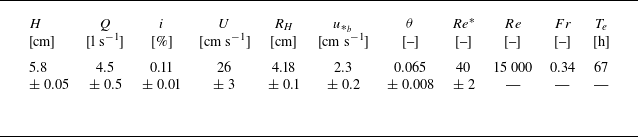
 H
 Q
 i
 U
 Q/(WH)
 W
 RH
 u∗b
 gRHi
 θ=u∗b2/(Δgd50)
 Re∗
 u∗bd50/ν
 Re
 HU/ν
 Fr
 U/gH
 Te

 k(x,y)=
 zb(x,y)
 zb
 t=50.2
 P=−zb/R
 ⟨P⟩x

 ⟨P⟩x
 t
 y

 ⟨P⟩
 E
 Cs
 E
 Cs
 EP0
 CP0
 ⟨P⟩

 zb
 W

 A
 B

 u¯
 w¯
 U
 A
 u¯
 w¯

 v¯/U
 A
 B

 τxz
 τP0
 τxz/τP0
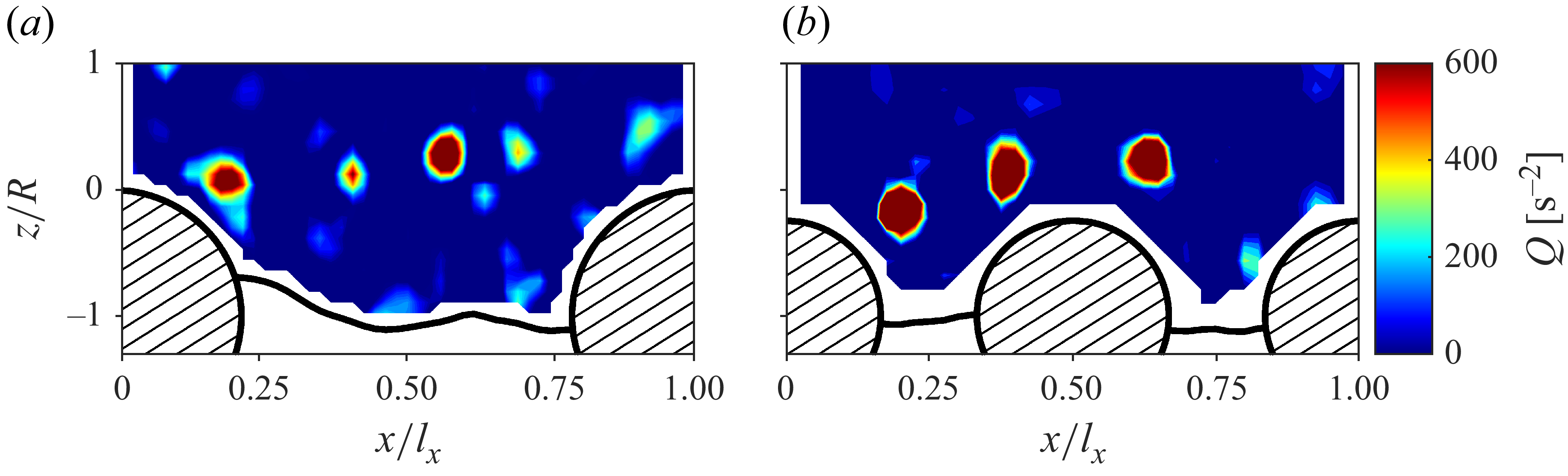
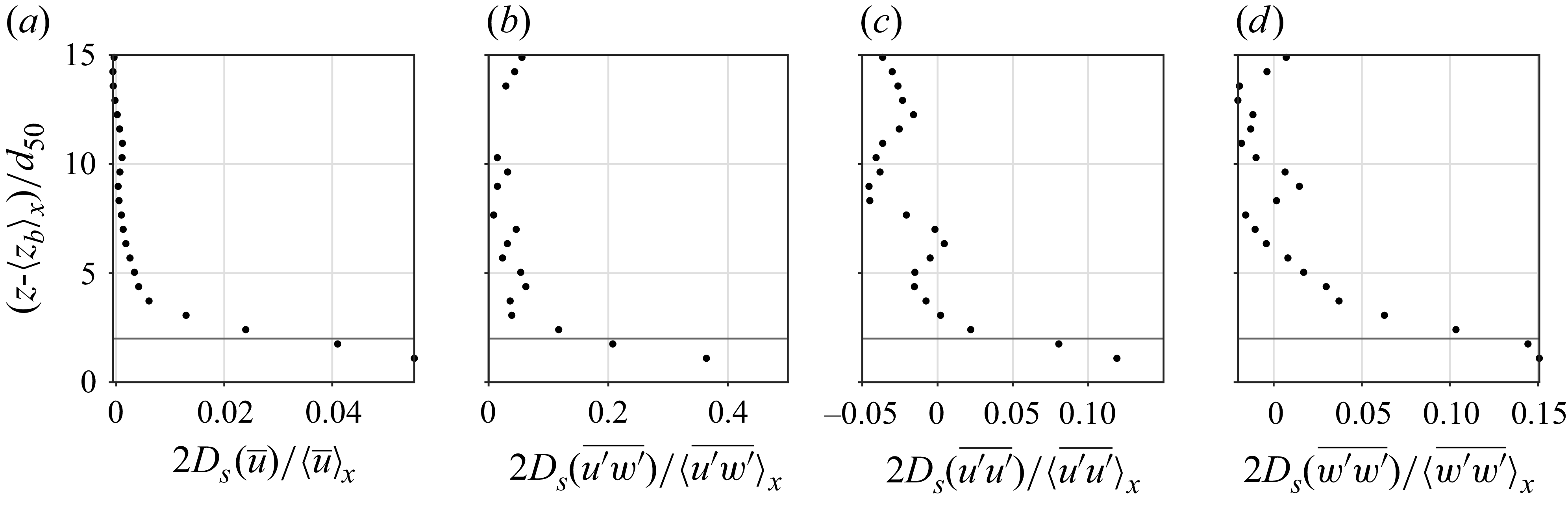
 Ds
 d50
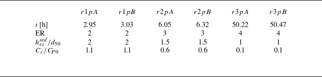
 hrssed
 Cs/CP0

 z′
 x′
 z−zb
 (x−lx/2)/b
 z′=hrssed
 ts
 z′
 hrssed
 αx

 Δθ
 −0.25

 u′
 w′
 d50
 d50
 A
 u′
 w′
 τxz
 u∗

 Pci
 αa
 λp

 ⟨zb⟩x
 y/W
 EP0
 ⟨τxz⟩x
 u∗P0
 ⟨τxz⟩x
 u′
 w′
 z=hrssed=2d50

 Open access

