1 Introduction
Turbulent wall layers are a pervasive feature in engineering and environmental flows. The relationship between the near-wall structures and the outer flow in these layers is of particular importance. This is because the former can be significantly altered by perturbations at the wall, such as those found in many practical flows in the form of surface roughness generated by defects, erosion and deposition, including that of living organisms.
Townsend (Reference Townsend1956) used simple dimensional arguments to demonstrate that on an outer domain where the direct influence of viscosity is negligible, the turbulent flow can depend only on the height of the wall layer and the wall stresses. The statement implies little consequence from near-wall modifications on outer-layer dynamics, other than that reflected in the appropriate length and velocity scales of the outer region. Where wall perturbations are present, similar arguments can be constructed, but similarity can only be anticipated external to perturbation-generated flow patterns. Therefore, in flows above perturbed walls an outer similarity region of measurable length is only plausible when the Reynolds number of the flow is high, and when the perturbation scale(s) are significantly smaller than the layer thickness. It is important to note here that, although commonly attempted in the literature, most perturbations cannot be characterised by a single scale – extreme examples are transverse bar/rod and highly directional or heterogeneous surfaces which can generate flow patterns significantly larger than their wall-normal perturbation height (see Volino, Schultz & Flack (Reference Volino, Schultz and Flack2011), Barros & Christensen (Reference Barros and Christensen2014), Anderson et al. (Reference Anderson, Barros, Christensen and Awasthi2015) and Vanderwel & Ganapathisubramani (Reference Vanderwel and Ganapathisubramani2015)). Here, we limit our discussion to studies above wall perturbations that are well-characterised; surfaces that are not known to produce disproportionately large flow patterns, and that have characteristic scales that are only a small fraction of the wall-layer thickness.
Investigations into the validity of Townsend’s hypothesis where the wall condition is modified (typically by roughening the bounding wall) are abundant in the literature. Many recent studies attempt to evaluate the effect of wall perturbations on the spatial structure of the outer flow. Allen et al. (Reference Allen, Shockling, Kunkel and Smits2007), Kunkel, Allen & Smits (Reference Kunkel, Allen and Smits2007) and Volino, Schultz & Flack (Reference Volino, Schultz and Flack2007), for example, demonstrate good agreement between smooth- and rough-wall streamwise wavelength spectra, particularly those of streamwise velocity fluctuations. Similar outer-layer agreement is observed by Chung, Monty & Ooi (Reference Chung, Monty and Ooi2014) in wavelength spectra from a turbulent channel flow direct numerical simulation (DNS) with no-slip and uniform shear-stress boundary conditions. These results, however, are contrasted by the smooth–rough-wall spectral comparisons of Krogstad, Antonia & Browne (Reference Krogstad, Antonia and Browne1992) and Krogstad & Antonia (Reference Krogstad and Antonia1999). In addition to differences in the magnitude of their compared spectra, Krogstad and colleagues demonstrate that their rough-wall spectra are generally shifted towards smaller wavelengths, particularly for spectra and co-spectra involving the wall-normal velocity component. Many other spatial investigations above well-characterised surface perturbations assess outer-layer structure in the context of the hairpin-packet paradigm, for which there is considerable evidence in smooth-wall flows (see Adrian, Meinhart & Tomkins Reference Adrian, Meinhart and Tomkins2000). Across these studies, there is generally agreement that the large-scale streamwise structure of rough- and smooth-wall boundary layers is qualitatively similar (see, for example Volino et al. (Reference Volino, Schultz and Flack2007) and Wu & Christensen (Reference Wu and Christensen2010)), but quantitative differences are noted in a number of cases. Krogstad & Antonia (Reference Krogstad and Antonia1994) and Volino et al. (Reference Volino, Schultz and Flack2007), for example, both report reductions in characteristic rough-wall velocity length scales, relative to those observed above smooth walls.
1.1 Relating time and space above perturbed walls
Many of the studies described in the previous paragraph deduce structural descriptions from temporally sampled point measurements. Exclusively, this is achieved using Taylor’s (Reference Taylor1938) hypothesis, which assumes that over the sampling time the turbulence is frozen and convected at the local mean streamwise velocity (see Zaman & Hussain (Reference Zaman and Hussain1981) for a derivation/description of the hypothesis). Posed originally for advected grid turbulence, early theoretical studies demonstrate some justification for the use of Taylor’s hypothesis in shear flows, but only for small wavelengths (Lin Reference Lin1953; Lumley Reference Lumley1965). Generally, the approach is considered to be substantially accurate for intermediate-scale streamwise motions (
 $\unicode[STIX]{x1D706}_{x}\lesssim 6\unicode[STIX]{x1D6FF}$
) in the outer layer of smooth-wall boundary layers, provided that the temporal fluctuations in the convecting frame are small – see, for example, Dennis & Nickels (Reference Dennis and Nickels2008), Geng et al. (Reference Geng, He, Wang, Xu, Lozano-Durán and Wallace2015) and de Kat & Ganapathisubramani (Reference de Kat and Ganapathisubramani2015). Near to the wall, structures are influenced by large-scale motions that are centred farther from the wall and so generally convect faster than the local mean (del Álamo & Jiménez Reference del Álamo and Jiménez2009). More accurate conversion between time and space in smooth-wall flows is obtained when the assumed convection velocity is determined as a function of location and scale (or frequency). Cenedese, Romano & Di Felice (Reference Cenedese, Romano and Di Felice1991) and Romano (Reference Romano1995), for example, use two-point laser Doppler anemometry measurements to quantify a frequency-dependent convection velocity that enables conversion between temporal and spatial descriptions of their turbulent channel flows. The latter show that when the convection velocity is characterised thus, the assumption that the turbulence is frozen can be considered generally appropriate in smooth-wall flows when the standard deviation of the streamwise velocity fluctuations is less than 30 % of the local streamwise velocity (that is,
 $\sqrt{\overline{u^{2}}}/U<0.3$
). Similarly, Lee, Lele & Moin (Reference Lee, Lele and Moin1992) report an approximate threshold of
 $\sqrt{\overline{u^{2}}}/U<15\,\%{-}25\,\%$
for incompressible isotropic turbulent flow using a similar quantification of the convection velocity.
There is significantly less justification for the application of the frozen turbulence hypothesis in flows above perturbed walls, where the turbulence intensities as a proportion of the local mean can be significantly higher. Squire et al. (Reference Squire, Morrill-Winter, Hutchins, Schultz, Klewicki and Marusic2016b
), for example, demonstrate that under identical wind tunnel operating conditions, roughening the bounding wall with sandpaper can cause a percentage increase in
 $\sqrt{\overline{u^{2}}}/U$
relative to the smooth wall of approximately 40 %, and that this percentage increase grows with roughness Reynolds number. Presuming then that
 $\sqrt{\overline{u^{2}}}/U$
provides a crude indication of the amplitude of temporal fluctuations in the convecting frame, it seems inevitable that the frozen turbulence assumption will become decreasingly accurate as roughness Reynolds number is increased, with an increasing proportion of the total energy in the temporal framework being aliased to erroneous wavelengths. Additionally, at high roughness Reynolds numbers, wall protrusions can generate stationary regions of low and high pressure – ‘residual stresses’ – in their wake. It is conceivable that these features could influence the advection of nearby events, especially given that under certain conditions these features will detach with regular frequency (see, for example, Bandyopadhyay Reference Bandyopadhyay1987). Presumably, however, the influence of stationary features above well-characterised rough surfaces is limited to within a few roughness heights from the wall.
There are a few notable studies that enable insight into the applicability of Taylor’s hypothesis in flows above perturbed walls. The conclusions of these studies, however, differ in this regard. Perry & Li (Reference Perry and Li1990) compare rough-wall spectra measured using a stationary hot-wire probe to those obtained by flying the probe through the same flow. When flying the hot-wire probe, the influence of temporal changes in the velocity field are less appreciable than for stationary measurements, so that a better measure of the spatial field is obtained. In agreement with the crude simulations of Perry, Henbest & Chong (Reference Perry, Henbest and Chong1986), Perry & Li (Reference Perry and Li1990) demonstrate that the application of Taylor’s hypothesis in rough-wall flows artificially redistributes energy to smaller wavelengths. This has interesting implications on the smooth- and rough-wall hot-wire measurements of Krogstad et al. (Reference Krogstad, Antonia and Browne1992) and Krogstad & Antonia (Reference Krogstad and Antonia1999) described above. However, the spectral comparisons of Perry & Li (Reference Perry and Li1990) indicate, assuming frozen turbulence, that the average convection velocity in the outer layer of their rough-wall flow is approximately twice the local mean velocity across all resolved scales. This equates to a convection velocity that is approximately equal to the free-stream velocity of the flow. Kaimal et al. (Reference Kaimal, Eversole, Lenschow, Stankov, Kahn and Businger1982) perform measurements in the atmospheric boundary layer over uneven terrain, covered with alternating patches of wheat stubble and winter wheat. They compare spectra obtained from stationary tower measurements, with those obtained from an aircraft bearing alongwind. While the aircraft and tower spectra are virtually indistinguishable for the streamwise velocity fluctuations, the tower spectra of the other velocity components are shifted towards larger wavelengths compared to the aircraft spectra, implying an average convection velocity that is less than the local mean velocity. Wilczek, Stevens & Meneveau (Reference Wilczek, Stevens and Meneveau2015) use large eddy simulation (LES) to resolve the wavenumber–frequency spectrum of the streamwise velocity in a rough-wall turbulent channel flow. They compare the true wavenumber spectrum with the wavenumber spectrum approximated from the frequency spectrum using Taylor’s hypothesis. The two spectra are very similar, except at small wavelengths. The small differences here, however, are assigned to ‘smearing’ in the frequency domain of the pronounced LES wavenumber cutoff, rather than to issues with Taylor’s approximation.
1.2 The present contribution
There are clearly ongoing questions in the literature regarding the influence of surface perturbations on the outer-region spatial structure of wall-bounded flows. Some of the confusion may arise from the application of Taylor’s hypothesis where the wall condition has negated the assumptions of the hypothesis. Here, we compare smooth- and rough-wall measurements at
 $\unicode[STIX]{x1D6FF}^{+}\approx 12\,000$
. The rough-wall measurements are obtained above a well-characterised surface roughness as described in Squire et al. (Reference Squire, Morrill-Winter, Hutchins, Schultz, Klewicki and Marusic2016a
) (sandpaper roughness:
 $k/\unicode[STIX]{x1D6FF}<1/380$
, where
 $k$
is the characteristic roughness height, and
 $\unicode[STIX]{x1D6FF}$
is the boundary layer thickness). For each wall condition, both temporal and true spatial descriptions of the same flow are compared – via hot-wire anemometry and high-spatial-range particle image velocimetry, respectively – enabling investigation of the applicability of Taylor’s hypothesis in the outer region. As will be shown, the application of Taylor’s hypothesis to the wall-normal velocity component produces inaccurate spatial estimates in the present rough-wall flow. Throughout this paper,
 $x$
,
 $y$
and
 $z$
denote the streamwise, spanwise and wall-normal directions. Mean and fluctuating (mean subtracted) quantities are denoted using uppercase and lowercase variables, respectively.
2 Experimental details
The present study utilises existing smooth- and rough-wall boundary layer data obtained using hot-wire anemometry (HWA) and particle image velocimetry (PIV). Key parameters of all experiments are provided in table 1. All measurements were carried out in the high Reynolds number boundary layer wind tunnel (HRNBLWT) at the University of Melbourne. The working section of this facility is 27 m long and has a cross-sectional area of approximately 2 m
 $\times$
1 m, producing moderate/high-Reynolds-number boundary layer flows with relatively large – and hence more readily resolvable – smallest energetic scales. Further details of the HRNBLWT are provided in Nickels et al. (Reference Nickels, Marusic, Hafez and Chong2005, Reference Nickels, Marusic, Hafez, Hutchins and Chong2007). The rough-wall measurements were performed above a single sheet of P36 grit sandpaper, covering the entire floor of the HRNBLWT test section. This rough surface has a physical roughness height
 $k=0.902$
mm and an equivalent sandgrain roughness height
 $k_{s}=1.96$
mm (Nikuradse Reference Nikuradse1933). For all rough-wall measurements presented herein,
 $z=z^{\prime }+\unicode[STIX]{x1D716}$
, where
 $z^{\prime }=0$
is located at the crest of the roughness, and
 $\unicode[STIX]{x1D716}$
is the wall offset parameter, required to account for the fact that the roughness displaces the entire flow outwards (Raupach, Antonia & Rajagopalan Reference Raupach, Antonia and Rajagopalan1991). As described in Squire et al. (Reference Squire, Morrill-Winter, Hutchins, Schultz, Klewicki and Marusic2016a
), the location of the local roughness crest is determined to within
 $\pm 25~\unicode[STIX]{x03BC}$
m, and the wall offset parameter is taken to be
 $\unicode[STIX]{x1D716}=0.902$
mm. No reasonable adjustment to
 $\unicode[STIX]{x1D716}$
can alter the results of the present study. A large floating element drag balance was used to determine
 $U_{\unicode[STIX]{x1D70F}}$
to within an accuracy of
 ${<}1\,\%$
for all rough-wall measurements (Baars et al.
Reference Baars, Squire, Talluru, Abbassi, Hutchins and Marusic2016). Further details of the rough surface are provided in Squire et al. (Reference Squire, Morrill-Winter, Hutchins, Schultz, Klewicki and Marusic2016a
).
Summary of the smooth (‘Sm.’) and rough (‘Ro.’) wall experiments. Note that
 $\widetilde{T}=TU_{\infty }/\unicode[STIX]{x1D6FF}\times 10^{-3}$
, where
 $T$
is the sampling time. T14, MW16 and S16b are abbreviations for Talluru et al. (Reference Talluru, Baidya, Hutchins and Marusic2014a
), Morrill-Winter et al. (Reference Morrill-Winter, Squire, Klewicki, Hutchins, Schultz and Marusic2016) and Squire et al. (Reference Squire, Morrill-Winter, Hutchins, Schultz, Klewicki and Marusic2016b
), respectively.

All HWA data were obtained using multiple-component probes that resolve at least the streamwise and wall-normal velocity components simultaneously. Note that the probe geometry was different for the smooth- and rough-wall measurements; for the smooth-wall case a conventional cross-wire probe was used, whereas the rough-wall HWA data were obtained using a four-wire probe similar in arrangement to that of Foss & Haw (Reference Foss and Haw1990), but significantly smaller in size. However, the wall-normal component in both cases is obtained from a similar viscous-scaled
 $\times$
-wire array. In identical flow conditions, both probes produce estimates of first- and second-order turbulence statistics that agree very well. Details of the calibration and operation of the smooth- and rough-wall HWA measurements are provided in Talluru et al. (Reference Talluru, Baidya, Hutchins and Marusic2014a
) and Morrill-Winter et al. (Reference Morrill-Winter, Klewicki, Baidya and Marusic2015), respectively. To briefly summarise, all probes were operated in constant temperature mode using a Melbourne University Constant Temperature Anemometer (MUCTA II) of in-house design. The hot-wire signals were filtered at the Nyquist frequency and were sampled using a 16-bit data-acquisition board. The diameter and length of the sensing element for all measurements were
 $d=2.5$
 $\unicode[STIX]{x03BC}$
m and
 $l=0.5$
mm, respectively. Full two-dimensional calibration was achieved in situ using an automated pitching jet, and the intermediate single-point recalibration technique was used to account for calibration drift during all measurements (Talluru et al.
Reference Talluru, Kulandaivelu, Hutchins and Marusic2014b
). For the latter, a stationary Pitot-static pair located in the free stream constituted the calibration standard. The PIV measurements employed here are described and validated in de Silva et al. (Reference de Silva, Gnanamanickam, Atkinson, Buchmann, Hutchins, Soria and Marusic2014) and Squire et al. (Reference Squire, Morrill-Winter, Hutchins, Schultz, Klewicki and Marusic2016b
), respectively, for the smooth and rough walls. All PIV data were obtained using an array of eight 14-bit PCO 4000 PIV cameras (CCD sensor:
 $2672\times 4008$
pixels), arranged in two horizontal rows. The combined field-of-view of this arrangement spans
 $L_{x}\approx 2\unicode[STIX]{x1D6FF}$
in the streamwise direction and resolves streamwise scales spanning well over two orders of magnitude. Note that the magnification of the top row of cameras is
 ${\sim}$
75 % of the bottom row. Thus, to approximately match spatial resolution (in wall units) across the entire field-of-view, the top cameras are processed using a correspondingly smaller pixel interrogation window size. Tracer particles were delivered by a Rosco smoke generator in the form of polyamide particles (diameter
 ${\approx}$
1
 $\unicode[STIX]{x03BC}$
m), and were illuminated using a Spectra Physics ‘Quanta-Ray’ PIV
 $400~\text{mJ}~\text{pulse}^{-1}$
Nd:YAG double-pulse laser.
As demonstrated in table 1, the data employed herein were all obtained at
 $\unicode[STIX]{x1D6FF}^{+}\approx 12\,000$
. Here, the boundary layer thickness,
 $\unicode[STIX]{x1D6FF}$
, was determined as the wall-normal location at which the mean streamwise velocity is 99 % of the free-stream velocity,
 $U_{\infty }$
. For each wall condition, we utilise data from HWA and PIV which were obtained under approximately matched wind tunnel operating conditions (streamwise location,
 $x$
, and free-stream velocity,
 $U_{\infty }$
). It is important to note, however, that the finite sensor size in HWA and PIV causes spatial attenuation of velocity measurements that differs between the two techniques – see Wyngaard (Reference Wyngaard1969) and Foucaut, Carlier & Stanislas (Reference Foucaut, Carlier and Stanislas2004) for discussions of the spatial attenuation resulting from each technique. The present PIV measurements were processed using an interrogation window size,
 $w_{Ix}^{+}\times w_{Iz}^{+}\approx 80\times 80$
(and laser sheet thickness
 $w_{Iy}^{+}\approx 20$
), whereas the wire length of the HWA probes was
 $l^{+}\approx 20$
. The latter satisfies the approximate guidelines laid out by Hutchins et al. (Reference Hutchins, Nickels, Marusic and Chong2009) for single wall-parallel wires to accurately resolve the streamwise turbulence intensity within the logarithmic region. However, the effect of finite dimensions differs for single- and multi-wire probes (Philip et al.
Reference Philip, Baidya, Hutchins, Monty and Marusic2013). Therefore, we emphasise only that we expect different degrees of spatial attenuation between the HWA and PIV measurements obtained under matched conditions – rows of table 1 – with the HWA data resolving more small-scale energy. When comparing smooth- and rough-wall data from a particular technique – columns of table 1 – the spatial resolutions are approximately matched, so a similar level of attenuation is expected.
3 Comparison of spectra
Recently, Morrill-Winter et al. (Reference Morrill-Winter, Squire, Klewicki, Hutchins, Schultz and Marusic2016) and Squire et al. (Reference Squire, Morrill-Winter, Hutchins, Schultz, Klewicki and Marusic2016a
) presented statistical and spectral comparisons between smooth-wall flow and the flow generated above the present surface roughness. Both studies exclusively employed temporal measurements and, where necessary, used Taylor’s hypothesis to approximate length scales. One aspect of the former work revealed that at matched friction Reynolds number and wallward of the logarithmic region, there are significant differences in the energy of streamwise velocity fluctuations between smooth- and rough-wall boundary layers in scales that are several
 $\unicode[STIX]{x1D6FF}$
in length. A similar observation was made by Monty et al. (Reference Monty, Allen, Lien and Chong2011), and is apparent in the smooth–rough comparisons of Rosenberg et al. (Reference Rosenberg, Hultmark, Vallikivi, Bailey and Smits2013).
Our approach to comparing the spatial structure of smooth- and rough-wall boundary layer flows is similar to these previous studies. Except where explicitly stated, Taylor’s hypothesis is used to present temporally sampled data in a spatial framework. However, here we investigate the energy of the streamwise and wall-normal velocity fluctuations, and incorporate comparisons to true spatial spectra obtained using PIV. Of course, the streamwise extent of the PIV (
 $L_{x}\approx 2\unicode[STIX]{x1D6FF}$
) is insufficient to resolve all scales for which Squire et al. (Reference Squire, Morrill-Winter, Hutchins, Schultz, Klewicki and Marusic2016a
) observed significant modification by the rough wall (in fact, their data indicate that this would require a streamwise extent of approximately
 $40\unicode[STIX]{x1D6FF}$
, which is very difficult and expensive to achieve using PIV at high Reynolds numbers). This is not to say that scales of length
 ${>}2\unicode[STIX]{x1D6FF}$
are not present in the PIV realisations, only that they cannot be fully resolved. The energy present in streamwise scales larger than the length of the field-of-view are present spectrally in the fluctuation of the local mean of a particular realisation about the global mean – that is, in the zeroth wavenumber, or D.C., Fourier mode (and, to some extent, leaked into the first few fully resolved modes). Therefore, limited investigation of these large-scale motions using the PIV data is still possible. In the following, all spectra are computed via fast Fourier transform. To avoid spatial aliasing of the PIV spectra, interrogation windows with 50 % overlap are used to attenuate aliased energy content above the Nyquist limit. Similarly, the analogue HWA signals are low-pass filtered at half of their sampling frequency (see table 1) prior to digitisation to avoid temporal aliasing. At each wall-normal height, the computed spectra are smoothed (Kaimal et al.
Reference Kaimal, Wyngaard, Izumi and Coté1972) and linearly interpolated onto 60 logarithmically spaced points in wavenumber space. Note that the results of the present study are not influenced by the smoothing or interpolation scheme, or by the number of interpolated points.
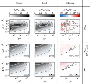
Comparison of the inner-normalised premultiplied energy spectrogram of streamwise velocity fluctuations,
 $k_{x}\unicode[STIX]{x1D6F7}_{uu}/U_{\unicode[STIX]{x1D70F}}^{2}$
, above the smooth (first column) and rough (second column) walls. The third column shows the difference between the smooth- and rough-wall spectrograms.
 $(a)$
Shows the full spectrograms computed using the HWA data;
 $(b)$
shows the spectrograms also computed using the HWA data, but processed in a similar manner to the PIV measurements (window size, overlap, and sampling frequency in the spatial framework); and
 $(c)$
shows the spectra from the PIV measurements. In
 $(a)$
, the vertical black hatched line shows the wall-normal location of the beginning of the logarithmic region according to the rough-wall formulation of Mehdi, Klewicki & White (Reference Mehdi, Klewicki and White2013) and the dashed box shows the flow domain resolved by the PIV. The datasets used in each plot are also indicated, in accord with table 1, by the symbol in the bottom right of each plot. Contour lines are shown in the first and second column in the range
 $k\unicode[STIX]{x1D6F7}_{uu}/U_{\unicode[STIX]{x1D70F}}^{2}=0.1{-}1.3$
with a spacing of 0.4, and in the third column in the range
 $k\unicode[STIX]{x1D6F7}_{uu}/U_{\unicode[STIX]{x1D70F}}^{2}|_{S-R}=0.02{-}0.38$
with a spacing of 0.12. Solid and dashed black lines are used to denote positive and negative contour levels, respectively.

3.1 Spectra of streamwise velocity fluctuations
The observations of Squire et al. (Reference Squire, Morrill-Winter, Hutchins, Schultz, Klewicki and Marusic2016a
) are reproduced using the present HWA data in figure 1(a), which shows the inner-normalised premultiplied spectrogram of the streamwise velocity fluctuations,
 $k_{x}\unicode[STIX]{x1D6F7}_{uu}/U_{\unicode[STIX]{x1D70F}}^{2}$
, obtained above the smooth wall (first column) and the rough wall (second column), and their subtracted difference (third column). In the latter, two key regions are highlighted. Close to the wall, roughness causes attenuation of inner-normalised streamwise energy relative to a smooth wall, which is well documented in the literature (Grass Reference Grass1971; Schultz & Flack Reference Schultz and Flack2007; Squire et al.
Reference Squire, Morrill-Winter, Hutchins, Schultz, Klewicki and Marusic2016a
). The attenuation is typically described as evidence for roughness-generated modifications to the near-wall cycle, which, in smooth-wall flows, is responsible for the inner (small-scale) energy peak. This description is appropriate for small-scale modifications close to the wall – see region
 $\unicode[STIX]{x2460}$
in the third column of figure 1(a). Region
 $\unicode[STIX]{x2461}$
indicates that there is an additional roughness influence far beyond the location of the smooth-wall energy peak, with a significant proportion of this influence in scales greater than approximately
 $2\unicode[STIX]{x1D6FF}$
. Squire et al. (Reference Squire, Morrill-Winter, Hutchins, Schultz, Klewicki and Marusic2016a
) demonstrated that the approximate edge of this region of influence coincides with the start of the logarithmic or inertial sublayer, beyond which, the smooth- and rough-wall energy are apparently equal. Mehdi et al. (Reference Mehdi, Klewicki and White2013) provide an empirical formulation for this location in rough-wall flows that is indicated by the black hatched lines in figure 1.
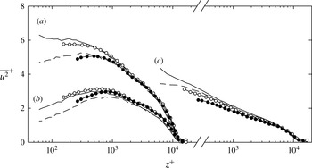
The variance of
 $u$
above smooth and rough walls: (a) the broadband variance profiles; (b) the variance profiles obtained subsequent to low-pass filtering with a cutoff wavelength equal to the streamwise extent of the PIV measurement; (c) the variance profiles obtained subsequent to high-pass filtering at the same cutoff wavelength. Symbols are defined in table 1. Note that the abscissa is shifted for plot (c).

Unfortunately, the present PIV measurements are incapable of resolving either of the regions described above, due to their limited streamwise extent and to laser reflection issues near to the wall (see Squire et al.
Reference Squire, Morrill-Winter, Hutchins, Schultz, Klewicki and Marusic2016b
). This is demonstrated by the dashed box in figure 1(a), which shows the range of wall-normal locations and streamwise scales fully resolved by the PIV measurements. The inner-normalised streamwise velocity spectra computed from the smooth- and rough-wall PIV data are presented in figure 1(c) following the same layout as figure 1(a). In figure 1(b), the HWA spectra are represented, but these are computed using a window size, overlap and sampling frequency in the spatial framework that are approximately equal to those used to compute the PIV spectra, thus assisting direct comparisons to the PIV spectra. Generally, the smooth- and rough-wall spectrograms, and their difference are similar for the HWA and PIV measurements (figures 1
b and 1
c), indicating that Taylor’s hypothesis is approximately appropriate for smooth- and rough-wall streamwise velocity fluctuations over the domain
 $z/\unicode[STIX]{x1D6FF}\gtrsim 0.02$
and
 $0.007\lesssim \unicode[STIX]{x1D706}_{x}/\unicode[STIX]{x1D6FF}\lesssim 2$
. These approximate bounds are limited by the resolved domain of the PIV measurements. Recall that due to spatial attenuation differences between the two techniques, small-scale differences between HWA and PIV spectra obtained under matched conditions are expected, with less energy resolved by the PIV. At the large scales, quantitative comparisons of the smooth, rough, HWA and PIV measurements are achievable through decomposition of the total energy into small- and large-scale contributions. These are presented in figure 2, which shows: (a), the total streamwise variance from the HWA and PIV measurements; (b), the low-pass filtered variance profiles, computed using a cutoff wavelength equal to the streamwise extent of the PIV measurement,
 $L_{cut}=L_{x}\approx 2\unicode[STIX]{x1D6FF}$
(i.e. removing small-scale contributions); and (c), the high-pass filtered profiles using the same cutoff wavelength. Note that the PIV profiles in figure 2(b) represent the energy associated with all scales longer than the streamwise extent of the PIV measurements, while those in figure 2(c) show the energy that is fully resolved by these measurements; addition of these contributions returns the broadband streamwise energy (variance) profiles in figure 2(a). Generally, predictions from HWA and PIV agree well. Comparing figures 2(a) and 2(c), it is clear that the PIV measurements only fully resolve scales that contribute to approximately half of the total variance, with the remaining energy residing in scales longer than
 $L_{x}$
. Near the wall, both measurement techniques demonstrate substantial differences between the smooth- and rough-wall broadband variance profiles (see figure 2
a). Both techniques also reveal in figure 2(b) that streamwise scales larger than
 $L_{x}$
are responsible for a large proportion of these differences. This is particularly remarkable given that the characteristic roughness scale is approximately 400 times smaller than
 $\unicode[STIX]{x1D6FF}$
, and yet the roughness appears to significantly influence the energy of streamwise motions that are longer than
 $2\unicode[STIX]{x1D6FF}$
(especially near the wall, where PIV data are not available – see the smooth- and rough-wall HWA spectra in figure 1
a). The energy contained in scales less than
 $L_{x}$
seems to be affected by the rough wall across the entire boundary layer. In figure 2(c), the smooth- and rough-wall profiles both show approximately log-linear decay absent large-scale contributions, and are consistent with the attached eddy hypothesis and its prediction of
 $k_{x}^{-1}$
spectral behaviour (Hutchins & Marusic Reference Hutchins and Marusic2007). However, the rough-wall energy is attenuated slightly below that of the smooth wall for both the HWA and PIV measurements. Considering the differenced spectrograms in figure 1(b,c), the attenuation of small-scale energy is apparently similar across all contributing scales. It is important to note, however, that the smooth–rough differences in figure 2(c) are small; comparable to the expected level of uncertainty in each measurement. This is discussed in detail in § 3.3.
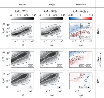
Inner-normalised premultiplied energy spectrograms of the wall-normal velocity fluctuations,
 $k_{x}\unicode[STIX]{x1D6F7}_{ww}/U_{\unicode[STIX]{x1D70F}}^{2}$
, plotted in the same format as figure 1. Contour lines are shown in the first and second column in the range
 $k\unicode[STIX]{x1D6F7}_{ww}/U_{\unicode[STIX]{x1D70F}}^{2}=0.07{-}0.29$
with a spacing of 0.11, and in the third column in the range
 $k\unicode[STIX]{x1D6F7}_{ww}/U_{\unicode[STIX]{x1D70F}}^{2}|_{S-R}=0.02{-}0.06$
with a spacing of 0.02. Solid and dashed black lines are used to denote positive and negative contour levels, respectively.

3.2 Spectra of wall-normal velocity fluctuations
In a similar manner to figure 1, figure 3 presents smooth- and rough-wall inner-normalised premultiplied spectrograms of the wall-normal velocity fluctuations,
 $k_{x}\unicode[STIX]{x1D6F7}_{ww}/U_{\unicode[STIX]{x1D70F}}^{2}$
from HWA and PIV. As before, figure 3(a,b) is computed using HWA data, while figure 3(c) shows PIV data. The HWA spectra in figure 3
 $(b)$
are computed using similar spectral processing parameters to those from the PIV. Generally, the smooth- and rough-wall HWA spectra appear qualitatively similar. However, their difference indicates that the spectral intensity in rough-wall flow is generally shifted to larger wavelengths across the entire boundary layer. This is demonstrated by the regions of positive and negative difference in the third column of figure 3(a) (regions
 $\unicode[STIX]{x2460}$
and
 $\unicode[STIX]{x2461}$
, respectively). Given that the smooth- and rough-wall inner-normalised variances approximately collapse, the observation implies that somehow the rough wall redistributes energy to larger scales but does not affect its total magnitude. We emphasise that this observation is robust over a range of matched Reynolds number smooth- and rough-wall HWA measurements, although, for brevity, these are not presented here. In contrast, figure 3(c) indicates that the smooth- and rough-wall spectrograms of wall-normal fluctuations obtained using PIV are similar in their distribution. Over the range of fully resolved scales, the PIV measurements indicate marginally less rough-wall energy than smooth-wall energy across the boundary layer. However, the difference is small and, considering how it is distributed in figure 3(c), it seems unlikely that the observed differences are physically meaningful. Note that the regions labelled
 $\unicode[STIX]{x2462}$
in figure 3(c) are not considered to represent real physical differences between smooth- and rough-wall energy. The top larger-wavelength region likely results from small errors in determining
 $\unicode[STIX]{x1D6FF}$
; this region can be removed by changing either the smooth- or rough-wall
 $\unicode[STIX]{x1D6FF}$
by only 1 %. The smaller-wavelength region appears for the range of wall-normal locations that are imaged by the lower row of cameras for the smooth-wall measurements, but the upper row for the rough-wall measurements. Thus, it may result from small differences in spatial resolution between the smooth- and rough-wall measurements across this region, and/or from low-level noise present in the top four cameras of the rough-wall measurement.
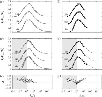
Profiles of the inner-normalised premultiplied energy spectra of wall-normal velocity fluctuations,
 $k_{x}\unicode[STIX]{x1D6F7}_{ww}/U_{\unicode[STIX]{x1D70F}}^{2}$
, in smooth- and rough-wall flows within the logarithmic region. (a) Compares Taylor-approximated spectra in smooth- and rough-wall flows; (b) compares PIV spectra in smooth- and rough-wall flows; (c) compares Taylor-approximated and PIV spectra in smooth-wall flows; and (d) compares Taylor-approximated and PIV spectra in rough-wall flows. Plots (e,f) show the difference,
 $D$
, between the Taylor-approximated and true spectra for the smooth and rough walls, respectively. Profiles are shown in all plots at: (i),
 $z/\unicode[STIX]{x1D6FF}\approx 0.05$
; (ii),
 $z/\unicode[STIX]{x1D6FF}\approx 0.1$
; (iii),
 $z/\unicode[STIX]{x1D6FF}\approx 0.14$
(note the arrows in (e,f) show increasing wall-normal location). The grey shaded region shows
 $\unicode[STIX]{x1D706}_{x}\lesssim 10w_{Ix}$
, where, recall,
 $w_{Ix}$
represents the interrogation window size of the PIV. Differences in spatial attenuation between the HWA and PIV measurements are expected to be negligible outside of this approximate region. Symbols are defined in table 1.

The behaviours described in the previous paragraph are perhaps better perceived in figures 4(a) and 4(b), which compare smooth- and rough-wall spectra,
 $k_{x}\unicode[STIX]{x1D6F7}_{ww}/U_{\unicode[STIX]{x1D70F}}^{2}$
, obtained from the HWA and PIV measurements, respectively. At each wall-normal location presented, the rough-wall HWA spectra of figure 4(a) are shifted towards larger wavelengths relative to the corresponding smooth-wall spectra. The same trend, however, is not apparent when comparing true spatial descriptions of the smooth- and rough-wall energy given in figure 4(b). In figure 4(c,d) the HWA and PIV spectra are compared for each wall condition. The grey shaded region shows
 $\unicode[STIX]{x1D706}_{x}\lesssim 10w_{Ix}$
, where, recall,
 $w_{Ix}$
represents the interrogation window size of the PIV. Differences in spatial attenuation between the HWA and PIV measurements are expected to be negligible outside of this approximate region. As is demonstrated in figure 4(c), the smooth-wall HWA and PIV spectra collapse well for scales larger than those strongly influenced by spatial attenuation of either measurement technique. Thus, the discrepancies observed between the HWA and PIV spectra in the third columns of figures 3(b) and 3(c), respectively, result primarily from differences between HWA and PIV spectra above the rough wall. This is demonstrated in figure 4(e,f), which shows the difference,
 $D$
, between the Taylor-approximated and true spectra for the smooth and rough walls, respectively. As is demonstrated in the Appendix, these general behaviours are also apparent from comparisons of
 $k_{x}\unicode[STIX]{x1D6F9}_{uw}/U_{\unicode[STIX]{x1D70F}}^{2}$
, again despite approximate agreement between all estimates of the smooth- and rough-wall Reynolds shear-stress profiles. Possible interpretations are considered in the following section.
3.3 Possible interpretations of results
Before considering the implications of the present observations on the use of Taylor’s hypothesis, we first note that, albeit small, the observed differences between temporal and spatial wall-normal velocity spectra cannot be explained by potential errors in
 $U_{\unicode[STIX]{x1D70F}}$
,
 $\unicode[STIX]{x1D716}$
and
 $\unicode[STIX]{x1D6FF}$
. Certainly, changing our estimate of
 $U_{\unicode[STIX]{x1D70F}}$
for the rough-wall PIV measurement by only
 $2\,\%$
results in outer-region collapse between smooth- and rough-wall PIV spectra across all fully resolved wavelengths. However, no reasonable adjustment of
 $U_{\unicode[STIX]{x1D70F}}$
can remove the apparent shift to larger wavelengths in the energy of rough-wall wall-normal fluctuations that was observed in the HWA measurements in figures 3 and 4. Similarly, it is not possible to adjust
 $\unicode[STIX]{x1D6FF}$
or
 $\unicode[STIX]{x1D716}$
in figure 3(a) to produce collapse of the smooth- and rough-wall spectra, since the former influences both the abscissa and the ordinate of these plots, and the latter is physically bounded between
 $\unicode[STIX]{x1D716}=0$
and
 $\unicode[STIX]{x1D716}=k$
(Jackson Reference Jackson1981).
Given these points, the results of figures 3 and 4 question the validity of Taylor’s hypothesis in flows above perturbed walls. Without spatio-temporal measurements, however, the precise nature of the violation cannot be determined. Rather, it can only be deduced that wall perturbations apparently influence the convection velocities of outer-region structures, and/or influence the temporal evolution of the flow. It is worth noting that, for the present rough-wall measurements, the streamwise turbulence intensity is as high as 22 % of the local mean velocity. This lies within the range of limits determined by Romano (Reference Romano1995) and Lee et al. (Reference Lee, Lele and Moin1992), where Taylor’s hypothesis was observed to break down in smooth-wall flows (
 $\sqrt{\overline{u^{2}}}/U<15\,\%{-}30\,\%$
). However, if wall perturbations further violate the assumption that the turbulence is frozen, one would expect that Taylor-advected spectra would be shifted to smaller wavelengths than true spatial spectra (the opposite is observed here). Because spatial and temporal descriptions of the same flow are available, it is possible to determine the time-to-length mapping such that the spatial spectrum can be recovered from the temporal spectrum in the rough-wall case. The approach is similar to those previously applied in smooth-wall flows – see del Álamo & Jiménez (Reference del Álamo and Jiménez2009), Monty & Chong (Reference Monty and Chong2009) and Chung & McKeon (Reference Chung and McKeon2010). We begin by defining the dispersion relation,
 $\unicode[STIX]{x1D714}_{c}(k_{x},z)$
from the spatial spectrum,
 $\unicode[STIX]{x1D6F7}(k_{x},z)$
, and temporal spectrum,
 $E(\unicode[STIX]{x1D714},z)$
, where
 $\unicode[STIX]{x1D714}$
represents frequency and
 $k_{x}=2\unicode[STIX]{x03C0}/\unicode[STIX]{x1D706}_{x}$
represents wavenumber;
 $$\begin{eqnarray}\unicode[STIX]{x1D6F7}(k_{x},z)\equiv \unicode[STIX]{x1D714}_{c}^{\prime }(k_{x},z)E(\unicode[STIX]{x1D714}_{c}(k_{x},z),z),\quad \text{where }\unicode[STIX]{x1D714}_{c}^{\prime }\equiv \,\text{d}\unicode[STIX]{x1D714}_{c}/\text{d}k_{x}.\end{eqnarray}$$
Following Chung & McKeon (Reference Chung and McKeon2010), a convection velocity can be defined in terms of the dispersion relation,
 $U_{c}(k_{x},z)=\unicode[STIX]{x1D714}_{c}(k_{x},z)/k_{x}$
, such that, under Taylor’s hypothesis,
 $\unicode[STIX]{x1D714}_{c}(k_{x},z)=\unicode[STIX]{x1D714}_{c,T}(k_{x},z)=U(z)k_{x}$
. In the present work, we introduce the variable
 $C(k_{x},z)$
, where
 $$\begin{eqnarray}\unicode[STIX]{x1D714}_{c}(k_{x},z)=C(k_{x},z)U(z)k_{x},\end{eqnarray}$$
and determine
 $C(k_{x},z)$
to minimise the difference between the left- and right-hand sides of (3.1). We emphasise that, in order to interpret
 $C(k_{x},z)U(z)$
as the mean convection velocity of the most energetic eddies with wavenumber
 $k_{x}$
, one must first neglect potential influences that are unrelated to variable convection velocity, which is particularly questionable in rough-wall flows. Additionally, using the present data,
 $C$
can be expressed only as a function of streamwise wavelength and wall-normal location. However, del Álamo & Jiménez (Reference del Álamo and Jiménez2009) demonstrate in smooth-wall flows that the convection velocity is at least a function of both streamwise and spanwise wavelength. Furthermore, energy at a single wavenumber can contribute to multiple frequencies (and vice versa), making the definition of a single scale-dependent convection velocity difficult (see McKeon & Sharma (Reference McKeon and Sharma2010), Higgins et al. (Reference Higgins, Froidevaux, Simeonov, Vercauteren, Barry and Parlange2012) and de Kat & Ganapathisubramani (Reference de Kat and Ganapathisubramani2015)). For these reasons, it is safest to interpret
 $C(k_{x},z)$
as a correction to Taylor’s hypothesis that, under the assumption that the turbulence is frozen, enables conversion between temporal and spatial descriptions of the flow above the present rough surface.
The correction,
 $C(k_{x},z)$
, required to minimise the difference between HWA and PIV spectra of the wall-normal velocity fluctuations under the assumption that the turbulence is frozen (see (3.1) and (3.2)). In (a), the correction is presented for the smooth-wall (
 $C_{S}$
) and rough-wall (
 $C_{R}$
) flows. Contour levels are shown at
 $C=0.67,0.80,0.90,1.11,1.25,1.5$
, where dashed and solid lines represent
 $C<1$
and
 $C>1$
, respectively. Hatched lines show the location of the maximum wavelength,
 $\unicode[STIX]{x1D706}_{x}=10w_{x}$
, for which
 $C$
is expected to be strongly influenced by spatial resolution differences between the HWA and PIV measurements. In (b), the HWA spectra from figure 3(b) are recomputed using the corrections
 $C_{S}$
and
 $C_{R}$
, where superscript
 $C$
indicates corrected quantities.

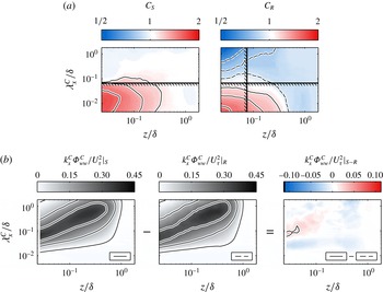
In figure 5(a),
 $C(\unicode[STIX]{x1D706}_{x},z)$
is presented for the smooth wall,
 $C_{S}$
, and the rough wall,
 $C_{R}$
. In each case,
 $C$
is deduced to minimise the error between the temporal HWA spectra,
 $E_{ww}(\unicode[STIX]{x1D714},z)$
, and the true spatial PIV spectra,
 $\unicode[STIX]{x1D6F7}_{ww}(k_{x},z)$
, according to (3.1) and (3.2), and is median-filtered using a kernel spanning approximately half an order of magnitude in each dimension to obtain a smooth estimate of
 $C$
(the discussions below are not influenced by this filtering). Where small-scale energy is present in the HWA spectra, this approach produces erroneous estimates of
 $C$
which reflect only the difference in the (spatial) attenuation resulting from the HWA and PIV measurements. This effect is responsible for the increase in
 $C_{S}$
and
 $C_{R}$
in small wavelengths near to the wall. As above, spatial resolution influences from either measurement technique are not expected for scales larger than
 $\unicode[STIX]{x1D706}_{x}\approx 10w_{x}$
, which is indicated by the horizontal hatched black lines in figure 5(a). The general behaviours of
 $C_{S}$
and
 $C_{R}$
can be predicted from the comparisons in figure 4(c,d). Because the smooth-wall Taylor-approximated HWA and PIV spectra collapse where spatial attenuation effects are negligible, a value of
 $C_{S}\approx 1$
is determined over this region. To relate HWA and PIV spectra above the rough wall, however,
 $C_{R}\approx 0.85$
is necessary in the outer layer (note that, as in figure 1, the vertical black hatched line in figure 5(a) shows the beginning of the logarithmic region according to the rough-wall formulation of Mehdi et al. (Reference Mehdi, Klewicki and White2013)). Under the assumption that the turbulence is frozen, this implies that the appropriate convection velocity over this region is approximately 85 % of the local mean streamwise velocity. In figure 5(b), the HWA spectra from figure 3(b) are recomputed using the corrections
 $C_{S}$
and
 $C_{R}$
. As previously, the first and second columns show the smooth- and rough-wall spectra, and the third column shows their difference. Evidently (and predictably), the estimated spatial spectra now indicate that the outer regions of the present rough- and smooth-wall flows are spatially similar, at least to the extent that can be determined from time-averaged spectra.
It is important to note that the streamwise and wall-normal velocity fluctuations need not necessarily follow the same dispersion relation; even if the turbulence were frozen, del Álamo & Jiménez (Reference del Álamo and Jiménez2009) show that the convection velocities of
 $u$
and
 $w$
motions differ. While it is indeed possible to determine new values for
 $C$
from
 $E_{uu}(\unicode[STIX]{x1D714},z)$
and
 $\unicode[STIX]{x1D6F7}_{uu}(k_{x},z)$
, these reveal only that, to within the experimental uncertainty of the present measurements, Taylor’s hypothesis is equally appropriate for streamwise velocity fluctuations in the outer region of the present smooth- and rough-wall flows. An important point should be made here. The subtle differences between the rough-wall HWA and PIV wall-normal velocity spectra in figure 4(d,f) are only distinct because the field-of-view of the PIV measurements is sufficient to resolve the majority of energy-containing scales associated with this component (in particular, sufficient to resolve the maxima of the energy spectra). Similar differences in the streamwise velocity spectra may be more difficult to observe since a large proportion of this spectra (including its maxima) is not resolved by the current PIV measurements. Direct spatial measurements that resolve the full range of energy-containing motions in rough-wall flows will provide insight in this regard, but such experiments remain inaccessible at high Reynolds numbers given the limited dynamic range of current PIV equipment.
3.4 A word of caution
The present paper demonstrates that there are apparent differences between Taylor-estimated spectra and true spatial spectra of the wall-normal velocity component in a rough-wall flow. These differences are not observed in the flow above a smooth wall. One possible interpretation of the result that
 $C_{R}<1$
in figure 5(a) is that our rough wall reduces the average convection velocity of outer-region energy-containing eddies. However, readers are warned that this interpretation inherently assumes that the turbulence is frozen, which is a questionable assumption even in smooth-wall flows (see, for example, del Álamo & Jiménez Reference del Álamo and Jiménez2009). It is also expected that the extent to which wall perturbations violate Taylor’s hypothesis depends on parameters associated with the roughness (for example,
 $k_{s}^{+}$
,
 $\unicode[STIX]{x1D6FF}/k_{s}$
, roughness morphology). Certainly, the present results and the study of Kaimal et al. (Reference Kaimal, Eversole, Lenschow, Stankov, Kahn and Businger1982) above distributed roughnesses indicate that the application of Taylor’s hypothesis in such flows can artificially redistribute energy to larger wavelengths. Perry & Li (Reference Perry and Li1990), however, deduce that the opposite occurs above mesh roughness. (Krogstad et al. (Reference Krogstad, Antonia and Browne1992) and Krogstad & Antonia (Reference Krogstad and Antonia1999) also scrutinise the flow above an expanded mesh roughness, reporting that their Taylor-approximated rough-wall spectra are generally shifted towards smaller wavelengths than corresponding smooth-wall measurements.) True spatio-temporal measurements (for example, time-resolved planar PIV) across a range of roughness parameters are required to shed light on the nature and causes of these observations. Nonetheless, the results of the present study, and indeed those listed above, indicate that care must be taken when deducing structural information from temporal measurements in rough-wall flows.
4 Conclusions
Temporally and spatially sampled measurements have been used to experimentally investigate the spatial structure of smooth- and rough-wall boundary layer flows at
 $\unicode[STIX]{x1D6FF}^{+}\approx 12\,000$
. This was achieved using hot-wire anemometry and particle image velocimetry, which were obtained at matched friction Reynolds numbers for each wall condition. The latter has a streamwise field-of-view spanning approximately
 $2\unicode[STIX]{x1D6FF}$
, thus limiting the maximum resolvable streamwise scale. The analysis involved comparison of smooth- and rough-wall spectra, and of true spatial spectra with those approximated from temporal data using Taylor’s (Reference Taylor1938) frozen turbulence hypothesis. Generally, the results of these comparisons can be summarised as follows.
-
(i) To within experimental uncertainty, there is agreement between Taylor-estimated and true spatial streamwise velocity spectra regardless of wall condition, indicating that Taylor’s hypothesis is generally appropriate for this velocity component over the resolved flow domain (
 $z/\unicode[STIX]{x1D6FF}\approx 0.02$
,
$\unicode[STIX]{x1D706}_{x}\lesssim 2\unicode[STIX]{x1D6FF}$
). The same is true for the wall-normal velocity spectra above the smooth wall. However, in the present rough-wall flow, clear differences are observed between the true spatial and temporally convected wall-normal velocity spectra, with the latter generally shifted towards larger wavelengths. This is perhaps foreseeable, given the high turbulence levels associated with the present rough-wall flow. A correction is proposed to enable accurate prediction of wall-normal velocity length scales from measurements of their time scales. Assuming that the turbulence is frozen, one interpretation of this correction is that the convection velocity in the outer region of the present rough-wall flow is generally less than the local mean streamwise velocity.
-
(ii) All true spatial spectra indicate outer-region structural similarity between smooth- and rough-wall flows. The same, of course, is true for temporal spectra when the above correction is applied to the wall-normal velocity component. There are substantial differences in the energy of streamwise velocity fluctuations between smooth- and rough-wall flows interior to the logarithmic region. Previous studies using HWA have demonstrated that streamwise scales larger than twice the boundary layer thickness are responsible for much of this difference. Unfortunately, the field of views of the present PIV measurements are insufficient to fully resolve scales this large. However, decomposition of the streamwise variance into scales
$\unicode[STIX]{x1D706}_{x}>2\unicode[STIX]{x1D6FF}$
demonstrate that large-scale near-wall energetic differences are also predicted by PIV measurements and are responsible for a large proportion of the total energy difference between the smooth- and rough-wall flows.


The implication that Taylor’s hypothesis can be inaccurate in rough-wall flows may help explain conflicting conclusions regarding the outer-region spatial structure of these flows. To fully understand the nature and causes of the present observations, however, spatio-temporal measurements in flows above perturbed walls are required.
Acknowledgements
The authors are grateful to the Australian Research Council for the financial support of this research, and to Dr R. Baidya and Dr C. de Silva for providing their smooth-wall HWA and PIV data. M. P. Schultz would like to thank the US Office of Naval Research for supporting his sabbatical visit to the University of Melbourne.
Appendix. Co-spectra of streamwise and wall-normal velocity fluctuations
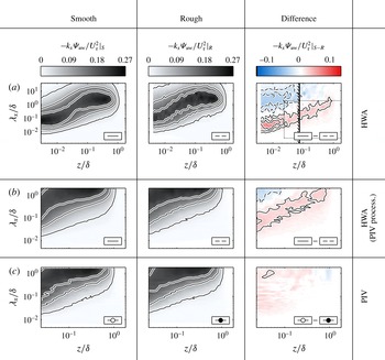
Discrepancies between Taylor-estimated and true spatial descriptions of rough-wall flows are also observed in the co-spectra of the streamwise and wall-normal velocity fluctuations. These are demonstrated in figure 6, which shows the PIV, HWA, smooth- and rough-wall co-spectra following the same layout as figures 1 and 3. As was observed for the wall-normal velocity spectra, subtraction of the Taylor-approximated smooth- and rough-wall co-spectra in figure 6(a) reveals distinct regions of positive and negative difference. However, such regions are apparently not observed for the true spatial measurements of the co-spectra in figure 6(c).
Inner-normalised premultiplied energy co-spectrograms of the streamwise and wall-normal velocity fluctuations,
 $-k_{x}\unicode[STIX]{x1D6F9}_{uw}/U_{\unicode[STIX]{x1D70F}}^{2}$
, plotted in the same format as figures 1 and 3. Contour lines are shown in the first and second column in the range
 $-k\unicode[STIX]{x1D6F9}_{uw}/U_{\unicode[STIX]{x1D70F}}^{2}=0.02{-}0.17$
with a spacing of 0.075, and in the third column in the range
 $-k\unicode[STIX]{x1D6F9}_{uw}/U_{\unicode[STIX]{x1D70F}}^{2}|_{S-R}=0.02{-}0.05$
with a spacing of 0.015. Solid and dashed black lines are used to denote positive and negative contour levels, respectively.