2 Double Beltrami states

The macroscopic evolution equations of the three dissipationless, collisionless and incompressible fluids read as

(2.1) $$\begin{eqnarray}\displaystyle & \displaystyle \frac{\unicode[STIX]{x2202}\boldsymbol{A}}{\unicode[STIX]{x2202}t}=\boldsymbol{V}_{+}\times \boldsymbol{B}-\unicode[STIX]{x1D735}\unicode[STIX]{x1D713}_{+}, & \displaystyle\end{eqnarray}$$

(2.2) $$\begin{eqnarray}\displaystyle & \displaystyle \frac{\unicode[STIX]{x2202}\boldsymbol{A}}{\unicode[STIX]{x2202}t}=\boldsymbol{V}_{-}\times \boldsymbol{B}+\unicode[STIX]{x1D735}\unicode[STIX]{x1D713}_{-}, & \displaystyle\end{eqnarray}$$

(2.3) $$\begin{eqnarray}\displaystyle & \displaystyle \frac{\unicode[STIX]{x2202}}{\unicode[STIX]{x2202}t}\left(\boldsymbol{V}_{i}+\boldsymbol{A}\right)=\boldsymbol{V}_{i}\times \left[\unicode[STIX]{x1D735}\times \boldsymbol{V}_{i}+\boldsymbol{B}\right]-\unicode[STIX]{x1D735}\unicode[STIX]{x1D713}_{i}, & \displaystyle\end{eqnarray}$$

where $\boldsymbol{V}_{j}\;(j=+,-,i)$ represents the velocity of the fluids normalized to the Alfvén velocity $V_{A}=B_{0}/\sqrt{\unicode[STIX]{x1D707}_{0}n_{i}m_{i}}$ ( $B_{0}$ is a constant magnetic field, $\unicode[STIX]{x1D707}_{0}$ is the permeability of free space, $n_{j}$ and $m_{j}$ represent the number densities and masses of the plasma species, respectively). The pressure of the species normalized to $B_{0}^{2}/\unicode[STIX]{x1D707}_{0}$ is represented by $p_{j}$ ; $\boldsymbol{E}$ is the electric field and satisfies the relation $\boldsymbol{E}=-\unicode[STIX]{x1D735}\unicode[STIX]{x1D719}-\unicode[STIX]{x2202}\boldsymbol{A}/\unicode[STIX]{x2202}t$ , $\unicode[STIX]{x1D719}$ is the scalar potential of the species normalized to $\unicode[STIX]{x1D706}_{i}B_{0}V_{A}$ and $\boldsymbol{A}$ is the vector potential $(\boldsymbol{B}=\unicode[STIX]{x1D735}\times \boldsymbol{A})$ normalized to  $\unicode[STIX]{x1D706}_{i}B_{0}$ . The magnetic field $\boldsymbol{B}$ is normalized to $B_{0}$ . All the distances are normalized to the ion skin depth $\unicode[STIX]{x1D706}_{i}=V_{A}/\unicode[STIX]{x1D714}_{c}=\sqrt{m_{i}/\unicode[STIX]{x1D707}_{0}n_{i}e^{2}}$ where  $\unicode[STIX]{x1D714}_{c}$ is the electron plasma frequency and $e$ is the elementary charge. Time is normalized to the inverse of the plasma frequency $\unicode[STIX]{x1D714}_{c}^{-1}=\unicode[STIX]{x1D706}_{i}/V_{A}$ . The scalars $(\unicode[STIX]{x1D713}_{j})$ in the gradient terms are $\unicode[STIX]{x1D713}_{+}=\unicode[STIX]{x1D719}+n_{i}p_{+}/n_{+}$ , $\unicode[STIX]{x1D713}_{-}=-\unicode[STIX]{x1D719}+n_{i}p_{-}/n_{-}$ and $\unicode[STIX]{x1D713}_{i}=\unicode[STIX]{x1D719}+\frac{1}{2}V_{i}^{2}+p_{i}$ . The pair particles are very much lighter and their masses have been ignored in comparison to the ions $(m\ll m_{i})$ in evaluating (2.1) and (2.2). The fluid pressures satisfy the relation $p_{j}=n_{j}T_{j}$ , where $T_{j}$ represents the temperature of the plasma species. The curls of (2.1), (2.2) and (2.3), yield respectively

(2.4) $$\begin{eqnarray}\displaystyle & \displaystyle \frac{\unicode[STIX]{x2202}\boldsymbol{B}}{\unicode[STIX]{x2202}t}=\unicode[STIX]{x1D735}\times [\boldsymbol{V}_{+}\times \boldsymbol{B}], & \displaystyle\end{eqnarray}$$

(2.5) $$\begin{eqnarray}\displaystyle & \displaystyle \frac{\unicode[STIX]{x2202}\boldsymbol{B}}{\unicode[STIX]{x2202}t}=\unicode[STIX]{x1D735}\times [\boldsymbol{V}_{-}\times \boldsymbol{B}], & \displaystyle\end{eqnarray}$$

(2.6) $$\begin{eqnarray}\displaystyle & \displaystyle \frac{\unicode[STIX]{x2202}}{\unicode[STIX]{x2202}t}(\unicode[STIX]{x1D735}\times \boldsymbol{V}_{i}+\boldsymbol{B})=\unicode[STIX]{x1D735}\times [\boldsymbol{V}_{i}\times (\unicode[STIX]{x1D735}\times \boldsymbol{V}_{i}+\boldsymbol{B})]. & \displaystyle\end{eqnarray}$$

These equations can be written in a more systematic form as

(2.7) $$\begin{eqnarray}\frac{\unicode[STIX]{x2202}\unicode[STIX]{x1D734}_{j}}{\unicode[STIX]{x2202}t}-\unicode[STIX]{x1D735}\times [\boldsymbol{U}_{j}\times \unicode[STIX]{x1D734}_{j}]=0,\end{eqnarray}$$

where $\unicode[STIX]{x1D734}_{j}\;(j=+,-,i)$ are the generalized vorticities $\unicode[STIX]{x1D734}_{-}=\unicode[STIX]{x1D734}_{+}=\boldsymbol{B}$ , $\unicode[STIX]{x1D734}_{i}=\unicode[STIX]{x1D735}\times \boldsymbol{V}_{i}+\boldsymbol{B}$ and $\boldsymbol{U}_{j}=\boldsymbol{V}_{j}$ are the effectual velocities. The general steady state solution of (2.7) is given by

(2.8) $$\begin{eqnarray}\boldsymbol{U}_{j}\times \unicode[STIX]{x1D734}_{j}=\unicode[STIX]{x1D735}\unicode[STIX]{x1D713}_{j},\end{eqnarray}$$

where $\unicode[STIX]{x1D713}_{j}\;(j=+,-,i)$ are the scalar fields and correspond to the energy densities of the fluids. The simplest equilibrium solution to (2.7) can be given in terms of the Beltrami condition, i.e. alignment of flows along the corresponding vorticities

(2.9) $$\begin{eqnarray}\unicode[STIX]{x1D734}_{j}=b_{j}\boldsymbol{U}_{j},\end{eqnarray}$$

where $b_{j}\;(j=+,-,i)$ are arbitrary constants and are referred to as the Beltrami parameters. Steady state solutions for the constituent fluids are, respectively,

(2.10) $$\begin{eqnarray}\displaystyle & \displaystyle b_{+}\boldsymbol{V}_{+}=\boldsymbol{B}, & \displaystyle\end{eqnarray}$$

(2.11) $$\begin{eqnarray}\displaystyle & \displaystyle b_{-}\boldsymbol{V}_{-}=\boldsymbol{B}, & \displaystyle\end{eqnarray}$$

(2.12) $$\begin{eqnarray}\displaystyle & \displaystyle b_{i}\boldsymbol{V}_{i}=\unicode[STIX]{x1D735}\times \boldsymbol{V}_{i}+\boldsymbol{B}. & \displaystyle\end{eqnarray}$$

The steady state solution shows that flows of pair particles follow the field lines while the ions follow the generalized vorticity (vorticity modified by the magnetic field). In order to find the magnetic field and velocities of the constituents, we make use of Ampere’s law which can be expressed as

(2.13) $$\begin{eqnarray}\boldsymbol{V}_{i}=\unicode[STIX]{x1D735}\times \boldsymbol{B}+\frac{\boldsymbol{V}_{-}}{N_{i}}-\frac{N_{+}}{N_{i}}\boldsymbol{V}_{+},\end{eqnarray}$$

where $N_{+}=n_{+}/n_{-}$ , and $N_{i}=n_{i}/n_{-}$ and we have taken into account the quasineutrality condition $n_{-}=n_{i}+n_{+}$ . Putting the value of $\boldsymbol{V}_{i}$ into (2.12), and using (2.10) and (2.11), we obtain

(2.14) $$\begin{eqnarray}(\unicode[STIX]{x1D735}\times )^{2}\boldsymbol{B}-a_{1}\unicode[STIX]{x1D735}\times \boldsymbol{B}+a_{0}\boldsymbol{B}=0,\end{eqnarray}$$

where

(2.15) $$\begin{eqnarray}\displaystyle & \displaystyle a_{0}=1-\frac{b_{i}}{N_{i}}\left(\frac{1}{b_{-}}-\frac{N_{+}}{b_{+}}\right)=1-\unicode[STIX]{x1D70C}b_{i}, & \displaystyle\end{eqnarray}$$

(2.16) $$\begin{eqnarray}\displaystyle & \displaystyle a_{1}=b_{i}-\frac{1}{N_{i}}\left(\frac{1}{b_{-}}-\frac{N_{+}}{b_{+}}\right)=b_{i}-\unicode[STIX]{x1D70C}, & \displaystyle\end{eqnarray}$$

and $\unicode[STIX]{x1D70C}=((1/b_{-})-(N_{+}/b_{+}))N_{i}^{-1}$ . Equation (2.14) is called a double Beltrami equation as it is equivalent to the linear sum of two Beltrami fields. It is worth noting that Beltrami conditions naturally give rise to the generalized Bernoulli condition ( $\unicode[STIX]{x1D713}_{j}=\text{const.}$ ). Putting the expressions (2.10)–(2.12) into the macroscopic evolution equations (2.1)–(2.3), we readily obtain

(2.17) $$\begin{eqnarray}\unicode[STIX]{x1D735}\unicode[STIX]{x1D713}_{j}=0,\end{eqnarray}$$

for steady state conditions. Integrating the above equation and introducing $\unicode[STIX]{x1D713}_{j}$ , we obtain

(2.18) $$\begin{eqnarray}\displaystyle & \displaystyle N_{i}p_{-}-\unicode[STIX]{x1D719}=g_{-}, & \displaystyle\end{eqnarray}$$

(2.19) $$\begin{eqnarray}\displaystyle & \displaystyle (N_{i}p_{+}/N_{+})+\unicode[STIX]{x1D719}=g_{+}, & \displaystyle\end{eqnarray}$$

(2.20) $$\begin{eqnarray}\displaystyle & \displaystyle (V_{i}^{2}/2)+p_{i}+\unicode[STIX]{x1D719}=g_{i}, & \displaystyle\end{eqnarray}$$

where $g_{j}\;(j=+,-,i)$ are arbitrary constants. Adding the above equations, we obtain

(2.21) $$\begin{eqnarray}\unicode[STIX]{x1D713}_{-}+\unicode[STIX]{x1D713}_{+}+\unicode[STIX]{x1D713}_{i}=g_{t},\end{eqnarray}$$

where $g_{t}=g_{-}+g_{+}+g_{i}$ . This equation can be written as

(2.22) $$\begin{eqnarray}N_{i}p_{-}+(N_{i}p_{+}/N_{+})+p_{i}+(V_{i}^{2}/2)+\unicode[STIX]{x1D719}=g_{t}.\end{eqnarray}$$

This shows that in the presence of a sheared flow, the system has the ability to confine an appreciable pressure (Mahajan & Yoshida Reference Mahajan and Yoshida1998, Reference Mahajan and Yoshida2000; Guzdar, Mahajan & Yoshida Reference Guzdar, Mahajan and Yoshida2005).

3 Root analysis

Equation (2.14) can also be expressed as

(3.1) $$\begin{eqnarray}(\unicode[STIX]{x1D735}\times )^{2}\boldsymbol{B}-(\unicode[STIX]{x1D706}+\unicode[STIX]{x1D707})\unicode[STIX]{x1D735}\times \boldsymbol{B}+\unicode[STIX]{x1D706}\unicode[STIX]{x1D707}\boldsymbol{B}=0,\end{eqnarray}$$

where $\unicode[STIX]{x1D706}$ and $\unicode[STIX]{x1D707}$ are taken as eigenvalues of the curl operator corresponding to two different eigenfunctions. Comparing (2.14) and (3.1), we obtain the following relations

(3.2) $$\begin{eqnarray}\displaystyle & \displaystyle \unicode[STIX]{x1D706}\unicode[STIX]{x1D707}=1-\unicode[STIX]{x1D70C}b_{i}, & \displaystyle\end{eqnarray}$$

(3.3) $$\begin{eqnarray}\displaystyle & \displaystyle \unicode[STIX]{x1D706}+\unicode[STIX]{x1D707}=b_{i}-\unicode[STIX]{x1D70C}. & \displaystyle\end{eqnarray}$$

The operators are commutative, the general solution of (2.14) can be written as

(3.4) $$\begin{eqnarray}\boldsymbol{B}=C_{\unicode[STIX]{x1D706}}\boldsymbol{F}_{\unicode[STIX]{x1D706}}+C_{\unicode[STIX]{x1D707}}\boldsymbol{F}_{\unicode[STIX]{x1D707}},\end{eqnarray}$$

where $\boldsymbol{F}_{\unicode[STIX]{x1D6FC}}$ (where $\unicode[STIX]{x1D6FC}=\unicode[STIX]{x1D706},\unicode[STIX]{x1D707}$ ) is the Beltrami field such that $\unicode[STIX]{x1D735}\times \boldsymbol{F}_{\unicode[STIX]{x1D6FC}}=\unicode[STIX]{x1D6FC}\boldsymbol{F}_{\unicode[STIX]{x1D6FC}}$ and $C_{\unicode[STIX]{x1D6FC}}$ are arbitrary constants. The eigenvalues of the curl operator are the roots of the quadratic equation

(3.5) $$\begin{eqnarray}\unicode[STIX]{x1D6FC}^{2}-a_{1}\unicode[STIX]{x1D6FC}+a_{0}=0,\end{eqnarray}$$

and read as

(3.6) $$\begin{eqnarray}\displaystyle & \displaystyle \unicode[STIX]{x1D706}=\frac{(b_{i}-\unicode[STIX]{x1D70C})+\sqrt{(b_{i}+\unicode[STIX]{x1D70C})^{2}-4}}{2}, & \displaystyle\end{eqnarray}$$

(3.7) $$\begin{eqnarray}\displaystyle & \displaystyle \unicode[STIX]{x1D707}=\frac{(b_{i}-\unicode[STIX]{x1D70C})-\sqrt{(b_{i}+\unicode[STIX]{x1D70C})^{2}-4}}{2}. & \displaystyle\end{eqnarray}$$

These are the roots of the DB field which is a superposition of two single Beltrami states. The roots may be real or complex. A mathematical treatment of the curl operators suggests that for a simply connected domain, the eigenvalues of the curl operator are real discrete numbers (Yoshida & Giga Reference Yoshida and Giga1990; Yoshida & Mahajan Reference Yoshida and Mahajan1999). The roots would be complex when the domain is multiply connected. The above expressions show that the scale parameters are functions of the Beltrami parameters and the number densities of the plasma species. The character of the roots of the quadratic equation (3.5) depends upon the discriminant ( $\unicode[STIX]{x1D6E5}$ ) which is defined as

(3.8) $$\begin{eqnarray}\unicode[STIX]{x1D6E5}=(b_{i}+\unicode[STIX]{x1D70C})^{2}-4.\end{eqnarray}$$

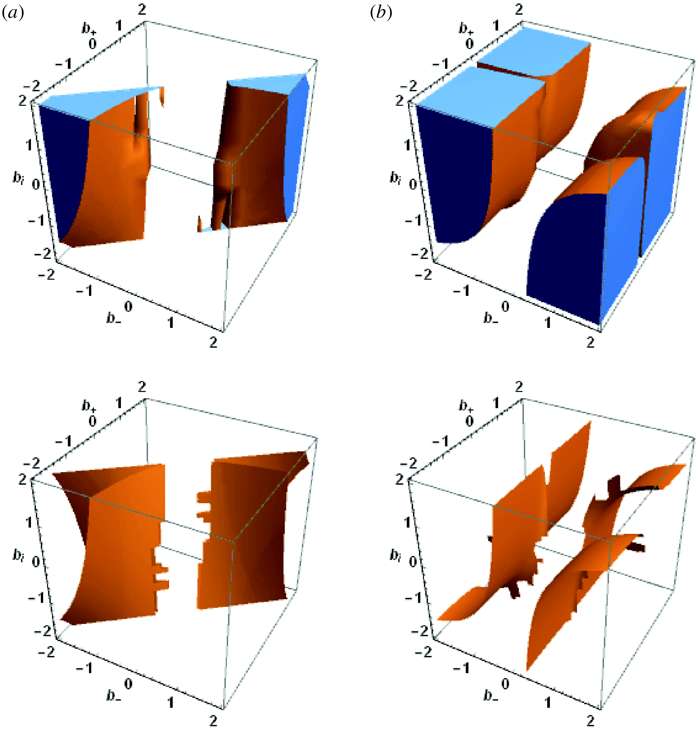
For $\unicode[STIX]{x1D6E5}<0$ or $b_{i}+\unicode[STIX]{x1D70C}<2$ , the roots are complex. The roots are degenerate when $\unicode[STIX]{x1D6E5}=0$ , i.e. when $b_{i}+\unicode[STIX]{x1D70C}=2$ . Both the scale parameters $\unicode[STIX]{x1D706}$ and $\unicode[STIX]{x1D707}$ become equal to $1-\unicode[STIX]{x1D70C}$ when $\unicode[STIX]{x1D6E5}=0$ . The impact of the number densities of the plasma constituents on the nature of the scale parameters and consequently on the formation of self-organized structures is shown in figure 1. Figure 1(a) shows the character of the eigenvalues as a function of the Beltrami parameters ( $b_{+},b_{-}$ and $b_{i}$ ) for $N_{i}=0.2$ . In this case, the electrons density is $5$ times greater than the ion density. On the other hand, figure 1(b) illustrates the character of the eigenvalues as a function of the Beltrami parameters ( $b_{+},b_{-}$ and $b_{i}$ ) for $N_{i}=0.9$ , that is $n_{i}=0.9n_{-}$ . The coloured regions of the graphs on the top show the regions where the scale parameters constitute a complex conjugate pair so that $|\unicode[STIX]{x1D706}|=|\unicode[STIX]{x1D707}|$ while the uncoloured regions show the points where they are real and distinct. On the other hand, the coloured region of the bottom graphs shows the points where the scale parameters become equal to each other $(\unicode[STIX]{x1D706}=\unicode[STIX]{x1D707})$ . The boundaries of the white regions coincide with the boundaries of the coloured region in the upper graphs, separating the scale parameter into two domains; one is the domain (white) where the eigenvalues are real while the other is the domain (coloured) where they become complex conjugate. The coloured region of the bottom graphs showing the degenerate roots are sandwiched between the coloured and white regions of the top graphs. Figure 1 shows that the densities of the species play a vital role in determining the character of the roots. It is evident that an increase in the density of ions strongly affects the scale parameters. Most of the real and distinct scale parameters are changed to complex conjugate pairs on increasing the ion density as compared to electrons, as shown in the top most graphs. The coloured portion increases with the increase in density in the top graphs which depicts that an increment of the ion density increases the complex eigenvalues. The degenerate roots also increases on an increase in the density of the ions, as shown in the bottom graphs.

Figure 1.

Character of the scale parameters of DB field as a function of the Beltrami parameters ( $b_{+},b_{-}$ and $b_{i}$ ) for (a) $N_{i}=0.2$ and (b) $N_{i}=0.9$ .

The explicit dependence of the scale parameters on the number densities is different from the scale parameters admitted by Hall MHD where only two species ions and inertialess electrons take part in the dynamics. The scale parameters of Hall MHD are independent of number density; they only depend on the Beltrami parameters which show the relation between flows and generalized vorticities only (Mahajan & Yoshida Reference Mahajan and Yoshida1998; Ohsaki et al. Reference Ohsaki, Shatashvili, Yoshida and Mahajan2001, Reference Ohsaki, Shatashvili, Yoshida and Mahajan2002). The formation of the self-organized structures and their features strongly depend on the scale parameters. Generally, the system will self-organize to a paramagnetic state when the scale parameters are real, to a diamagnetic state when they are complex and to a perfectly diamagnetic one when they are purely imaginary. For the real eigenvalues, the solution is expressed in terms of trigonometric functions in Cartesian coordinates which are oscillatory and generally we obtain the paramagnetic structures. On the other hand, when the eigenvalues of the curl operator are complex, the solution consists of hyperbolic functions which increase away from the centre and thus the magnetic field shows diamagnetic behaviour. Hence, it is expected that the number densities of the plasma components will play a role on a par with the flows and vorticities in the dynamics of multi-component plasmas. Eliminating $b_{i}$ from (3.2) and (3.3), we obtain

(3.9) $$\begin{eqnarray}(\unicode[STIX]{x1D706}+\unicode[STIX]{x1D70C})(\unicode[STIX]{x1D707}+\unicode[STIX]{x1D70C})=1.\end{eqnarray}$$

The Beltrami parameter can be written in terms of the scale parameters $\unicode[STIX]{x1D706}$  and $\unicode[STIX]{x1D707}$ . We have only two equations and there are three Beltrami parameters, therefore, we take one of the Beltrami parameters $b_{+}$ as constant and solve the equations for the two other parameters. After some algebraic manipulation, we obtain

(3.10) $$\begin{eqnarray}\tilde{b}_{-}=\frac{N_{+}}{b_{+}}-\left[\frac{\unicode[STIX]{x1D706}+\unicode[STIX]{x1D707}\mp \sqrt{(\unicode[STIX]{x1D706}-\unicode[STIX]{x1D707})^{2}+4}}{2}\right]N_{i},\end{eqnarray}$$

where $\tilde{b}_{-}=1/b_{-}$ . Solving (3.2) and (3.3), we obtain

(3.11) $$\begin{eqnarray}b_{i}=\frac{\unicode[STIX]{x1D706}+\unicode[STIX]{x1D707}\pm \sqrt{(\unicode[STIX]{x1D706}-\unicode[STIX]{x1D707})^{2}+4}}{2}.\end{eqnarray}$$

The composite velocity of the system reads as

(3.12) $$\begin{eqnarray}\unicode[STIX]{x1D70C}_{t}\boldsymbol{V}=\unicode[STIX]{x1D70C}_{i}\boldsymbol{V}_{i}+\unicode[STIX]{x1D70C}_{+}\boldsymbol{V}_{+}+\unicode[STIX]{x1D70C}_{-}\boldsymbol{V}_{-},\end{eqnarray}$$

where $\unicode[STIX]{x1D70C}_{t}=\unicode[STIX]{x1D70C}_{i}+\unicode[STIX]{x1D70C}_{+}+\unicode[STIX]{x1D70C}_{-}$ and $\unicode[STIX]{x1D70C}_{j}=m_{j}n_{j}\;(j=+,-,i)$ . As the masses of the positrons and electrons are neglected in comparison to the ions, therefore $\unicode[STIX]{x1D70C}_{+}=\unicode[STIX]{x1D70C}_{-}=0$ and the composite velocity $\boldsymbol{V}\approx \boldsymbol{V}_{i}$ . The composite velocity using (2.13) reads as

(3.13) $$\begin{eqnarray}\boldsymbol{V}=(\unicode[STIX]{x1D706}+\unicode[STIX]{x1D70C})C_{\unicode[STIX]{x1D706}}\boldsymbol{F}_{\unicode[STIX]{x1D706}}+(\unicode[STIX]{x1D707}+\unicode[STIX]{x1D70C})C_{\unicode[STIX]{x1D707}}\boldsymbol{F}_{\unicode[STIX]{x1D707}}.\end{eqnarray}$$

The loss of equilibrium gives rise to eruption and eruptive events are ubiquitous in space plasmas such as solar flares, eruptive prominences and coronal mass ejections in the solar atmosphere. The current system can lose equilibrium if either the scale parameters $\unicode[STIX]{x1D6FC}\;(\unicode[STIX]{x1D6FC}=\unicode[STIX]{x1D706},\unicode[STIX]{x1D707})$ go from real to complex or any one of the amplitudes $C_{\unicode[STIX]{x1D6FC}}$  ( $\unicode[STIX]{x1D6FC}=\unicode[STIX]{x1D706},\unicode[STIX]{x1D707}$ ) becomes complex. In order to investigate the possibility of the occurrence of sudden eruptive and catastrophic events within the framework of our approach, we assume a quasi-equilibrium state of a self-organized structure where the DB state is changing very slowly. The change is sufficiently slow so that the system remains in its local DB equilibrium. Equation (3.4) shows that the DB field depends on four physical parameters: two scale parameters $\unicode[STIX]{x1D6FC}^{\prime }s$ and two amplitudes $C_{\unicode[STIX]{x1D6FC}}$ . In order to find these parameters, we invoke the constants of motion following the work of Yoshida et al. (Reference Yoshida, Mahajan, Ohsaki, Iqbal and Shatashvili2001). To do so, first we need to know the constants of motion permitted by this system.

4 Constants of motion

Using (2.7) under appropriate boundary conditions (Steinhauer & Ishida Reference Steinhauer and Ishida1997; Mahajan & Yoshida Reference Mahajan and Yoshida1998, Reference Mahajan and Yoshida2000), it is straightforward to show that three helicities

(4.1) $$\begin{eqnarray}\displaystyle & \displaystyle h_{-}=\frac{1}{2}\int (\boldsymbol{A}\boldsymbol{\cdot }\boldsymbol{B})\,\text{d}v, & \displaystyle\end{eqnarray}$$

(4.2) $$\begin{eqnarray}\displaystyle & \displaystyle h_{+}=\frac{1}{2}\int (\boldsymbol{A}\boldsymbol{\cdot }\boldsymbol{B})\,\text{d}v, & \displaystyle\end{eqnarray}$$

(4.3) $$\begin{eqnarray}\displaystyle & \displaystyle h_{i}=\frac{1}{2}\int (\boldsymbol{A}+\boldsymbol{V})\boldsymbol{\cdot }(\boldsymbol{B}+\unicode[STIX]{x1D735}\times \boldsymbol{V})\,\text{d}v, & \displaystyle\end{eqnarray}$$

and the energy

(4.4) $$\begin{eqnarray}E=\frac{1}{2}\int (\boldsymbol{B}^{2}+\boldsymbol{V}_{i}^{2})\,\text{d}v,\end{eqnarray}$$

serve as constants of motion and remain invariant in time.

5 Conservation laws and DB parameters

The self-organized state of a two-fluid MHD plasma was derived by Steinhauer and Ishida (Steinhauer & Ishida Reference Steinhauer and Ishida1997, Reference Steinhauer and Ishida1998) using the variational principle where the total energy $E$ and two helicities are considered to evaluate the Euler–Lagrange equation. The double Beltrami self-organized state of a Hall MHD plasma has also been derived by Yoshida & Mahajan (Reference Yoshida and Mahajan2002) using the variational principle where the total energy $E$ , magnetic helicity and generalized helicity are taken to be constants. In the present system, the magnetofluid energy $(E)$ and helicities $(h_{j},j=+,-,i)$ for each plasma component act as constants of motion. The helicities for pair particles $h_{+}$ and $h_{-}$ are equal and in what follows we take $h_{+}=h_{-}=h$ . Hence the present system allows effectively three constants of motion just like that of Hall MHD (Ohsaki et al. Reference Ohsaki, Shatashvili, Yoshida and Mahajan2001, Reference Ohsaki, Shatashvili, Yoshida and Mahajan2002). It is easy to find out the algebraic relations for the constant of motions in terms of the scale parameters $\unicode[STIX]{x1D6FC}$ and $C_{\unicode[STIX]{x1D6FC}}$ . For this purpose, we choose $\unicode[STIX]{x1D706}$ as a control parameter and assume $|\unicode[STIX]{x1D706}|<|\unicode[STIX]{x1D707}|$ , that is $\unicode[STIX]{x1D706}$ specifies the large scale structure. We take a cube of length $L$ and consider a two-dimensional ABC field $\boldsymbol{F}_{\unicode[STIX]{x1D6FC}}\;(\unicode[STIX]{x1D6FC}=\unicode[STIX]{x1D706},\unicode[STIX]{x1D707})$ as expressed below

(5.1) $$\begin{eqnarray}\boldsymbol{F}_{\unicode[STIX]{x1D6FC}}=f_{\unicode[STIX]{x1D6FC}}^{x}\left(\begin{array}{@{}c@{}}0\\ \sin (\unicode[STIX]{x1D6FC}x)\\ \cos (\unicode[STIX]{x1D6FC}x)\end{array}\right)+f_{\unicode[STIX]{x1D6FC}}^{y}\left(\begin{array}{@{}c@{}}\cos (\unicode[STIX]{x1D6FC}y)\\ 0\\ \sin (\unicode[STIX]{x1D6FC}y)\end{array}\right),\end{eqnarray}$$

where $f_{\unicode[STIX]{x1D6FC}}^{x}$ and $f_{\unicode[STIX]{x1D6FC}}^{y}$ are constants and satisfy the relation $(f_{\unicode[STIX]{x1D6FC}}^{x})^{2}+(f_{\unicode[STIX]{x1D6FC}}^{y})^{2}=1$ . We assume $L=2\unicode[STIX]{x03C0}n_{\unicode[STIX]{x1D6FC}}/\unicode[STIX]{x1D6FC}$ , where $n_{\unicode[STIX]{x1D6FC}}$ are integers $(\unicode[STIX]{x1D6FC}=\unicode[STIX]{x1D706},\unicode[STIX]{x1D707})$ . We will consider only real $\unicode[STIX]{x1D6FC}$ and assume $L$ to be sufficiently large for $\unicode[STIX]{x1D6FC}\;(=2\unicode[STIX]{x03C0}n_{\unicode[STIX]{x1D6FC}}/L)$ to take continuous real values. The values of $\boldsymbol{F}_{\unicode[STIX]{x1D6FC}}$ also satisfy the following relations: $\int \boldsymbol{F}_{\unicode[STIX]{x1D6FC}}^{2}\,\text{d}r=L^{2}$ , and $\int \boldsymbol{F}_{\unicode[STIX]{x1D706}}\boldsymbol{\cdot }\boldsymbol{F}_{\unicode[STIX]{x1D707}}\,\text{d}r=0$ , where $\int \text{d}r=\int _{0}^{L}\int _{0}^{L}\,\text{d}x\,\text{d}y$ . The integrals of motion comes out to be

(5.2) $$\begin{eqnarray}\displaystyle & \displaystyle h=\frac{L^{2}}{2}\left(\frac{C_{\unicode[STIX]{x1D706}}^{2}}{\unicode[STIX]{x1D706}}+\frac{C_{\unicode[STIX]{x1D707}}^{2}}{\unicode[STIX]{x1D707}}\right) & \displaystyle\end{eqnarray}$$

(5.3) $$\begin{eqnarray}\displaystyle & \displaystyle h_{i}=\frac{L^{2}}{2}\left[\frac{C_{\unicode[STIX]{x1D706}}^{2}}{\unicode[STIX]{x1D706}}\left(\unicode[STIX]{x1D706}^{2}+\unicode[STIX]{x1D70C}\unicode[STIX]{x1D706}+1\right)^{2}+\frac{C_{\unicode[STIX]{x1D707}}^{2}}{\unicode[STIX]{x1D707}}\left(\unicode[STIX]{x1D707}^{2}+\unicode[STIX]{x1D70C}\unicode[STIX]{x1D707}+1\right)^{2}\right], & \displaystyle\end{eqnarray}$$

(5.4) $$\begin{eqnarray}\displaystyle & \displaystyle E=\frac{L^{2}}{2}\left[\left(1+\left(\unicode[STIX]{x1D706}+\unicode[STIX]{x1D70C}\right)^{2}\right)C_{\unicode[STIX]{x1D706}}^{2}+\left(1+\left(\unicode[STIX]{x1D707}+\unicode[STIX]{x1D70C}\right)^{2}\right)C_{\unicode[STIX]{x1D707}}^{2}\right]. & \displaystyle\end{eqnarray}$$

In what follows, we take

(5.5) $$\begin{eqnarray}\tilde{h}_{i}=h_{i}-h.\end{eqnarray}$$

Putting (5.2)–(5.3) into (5.5), and after some calculation, we obtain the following relation

(5.6) $$\begin{eqnarray}\tilde{h}_{i}=b_{i}E-\unicode[STIX]{x1D706}\unicode[STIX]{x1D707}h.\end{eqnarray}$$

Using (3.2) and eliminating $\tilde{h}_{i}$ from the above equations (5.5) and (5.6), we have

(5.7) $$\begin{eqnarray}b_{i}=\frac{h_{i}}{E+\unicode[STIX]{x1D70C}h}.\end{eqnarray}$$

Putting value of $b_{i}$ from (3.11) into (5.6), $\tilde{h}_{i}$ becomes

(5.8) $$\begin{eqnarray}\tilde{h}_{i}=\frac{E}{2}\left[\left(\unicode[STIX]{x1D706}+\unicode[STIX]{x1D707}\right)\pm \sqrt{\left(\unicode[STIX]{x1D706}-\unicode[STIX]{x1D707}\right)^{2}+4}\right]-\unicode[STIX]{x1D706}\unicode[STIX]{x1D707}h.\end{eqnarray}$$

After normalizing out the common factor $L^{2}/2$ , we obtain

(5.9) $$\begin{eqnarray}\displaystyle & \displaystyle C_{\unicode[STIX]{x1D706}}^{2}=\frac{\unicode[STIX]{x1D706}}{D}\left[E-h\unicode[STIX]{x1D707}\left\{1+\left(\unicode[STIX]{x1D707}+\unicode[STIX]{x1D70C}\right)^{2}\right\}\right], & \displaystyle\end{eqnarray}$$

(5.10) $$\begin{eqnarray}\displaystyle & \displaystyle C_{\unicode[STIX]{x1D707}}^{2}=\frac{\unicode[STIX]{x1D707}}{D}\left[-E+h\unicode[STIX]{x1D706}\left\{1+\left(\unicode[STIX]{x1D706}+\unicode[STIX]{x1D70C}\right)^{2}\right\}\right], & \displaystyle\end{eqnarray}$$

where

(5.11) $$\begin{eqnarray}\displaystyle D & = & \displaystyle \unicode[STIX]{x1D706}\left[1+\left(\unicode[STIX]{x1D706}+\unicode[STIX]{x1D70C}\right)^{2}\right]-\unicode[STIX]{x1D707}\left[1+\left(\unicode[STIX]{x1D707}+\unicode[STIX]{x1D70C}\right)^{2}\right],\end{eqnarray}$$

(5.12) $$\begin{eqnarray}\displaystyle & = & \displaystyle (\unicode[STIX]{x1D706}-\unicode[STIX]{x1D707})b_{i}(b_{i}+\unicode[STIX]{x1D70C}),\end{eqnarray}$$

which shows that $D=0$ for $\unicode[STIX]{x1D706}=\unicode[STIX]{x1D707}$ .

Figure 2.

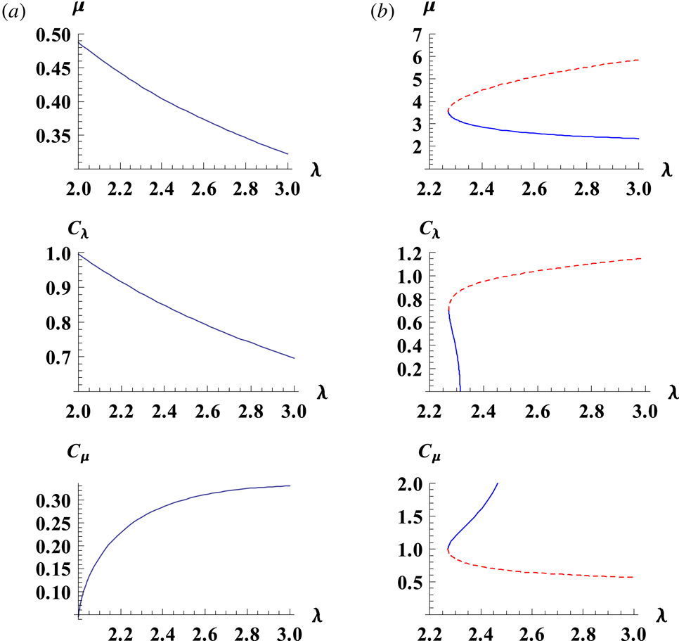
(a) Plots of $\unicode[STIX]{x1D707}$ , $C_{\unicode[STIX]{x1D706}}$ and $C_{\unicode[STIX]{x1D707}}$ versus $\unicode[STIX]{x1D706}$ for the densities of the plasma components $N_{i}=0.01$ , no catastrophe. (b) Plots of $\unicode[STIX]{x1D707}$ , $C_{\unicode[STIX]{x1D706}}$ and $C_{\unicode[STIX]{x1D707}}$ versus $\unicode[STIX]{x1D706}$ for $N_{i}=0.99$ . The equilibrium is lost at the critical point $\unicode[STIX]{x1D706}_{\text{crit}}\simeq 2.24$ . The energy of the plasma system $E=5.0$ , helicities $h=0.5$ and $h_{i}=5.0$ and the Beltrami parameter $b_{+}=0.2$ are taken as constant for both cases.

Figure 3.

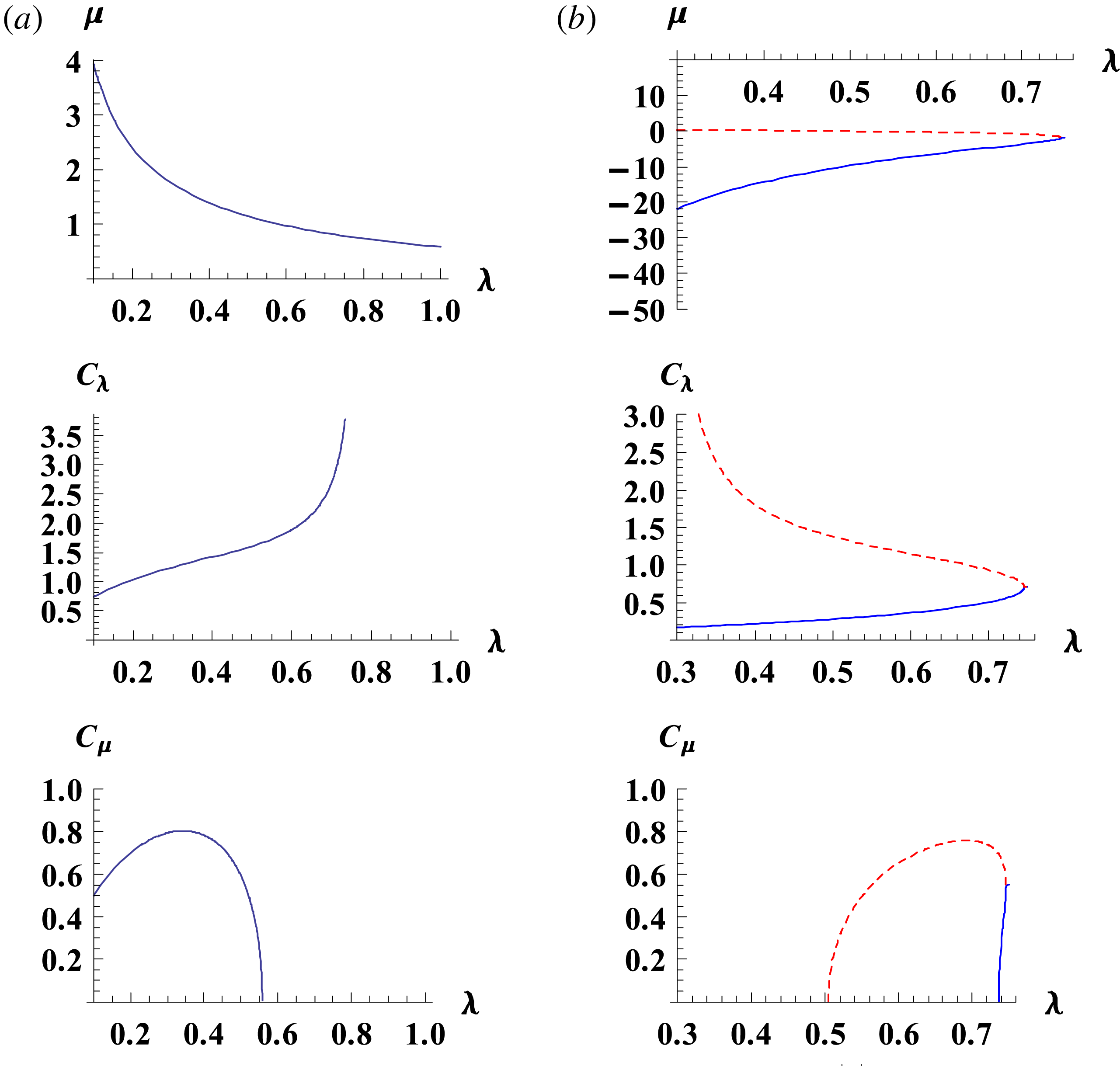
(a) Plots of $\unicode[STIX]{x1D707}$ , $C_{\unicode[STIX]{x1D706}}$ and $C_{\unicode[STIX]{x1D707}}$ versus $\unicode[STIX]{x1D706}$ for the helicities of the pair components of the plasma $h=5.5$ , no catastrophe. (b) Plots of $\unicode[STIX]{x1D707}$ , $C_{\unicode[STIX]{x1D706}}$ and $C_{\unicode[STIX]{x1D707}}$ versus $\unicode[STIX]{x1D706}$ for $h=0.5$ . The equilibrium is lost at the critical point $\unicode[STIX]{x1D706}_{\text{crit}}\simeq 0.75$ . The densities of the components $N_{i}=0.77$ , energy of the plasma system $E=5.0$ , helicity of the ions $h_{i}=5.0$ and the Beltrami parameter $b_{+}=0.2$ are taken as constant for both cases.

Figure 4.

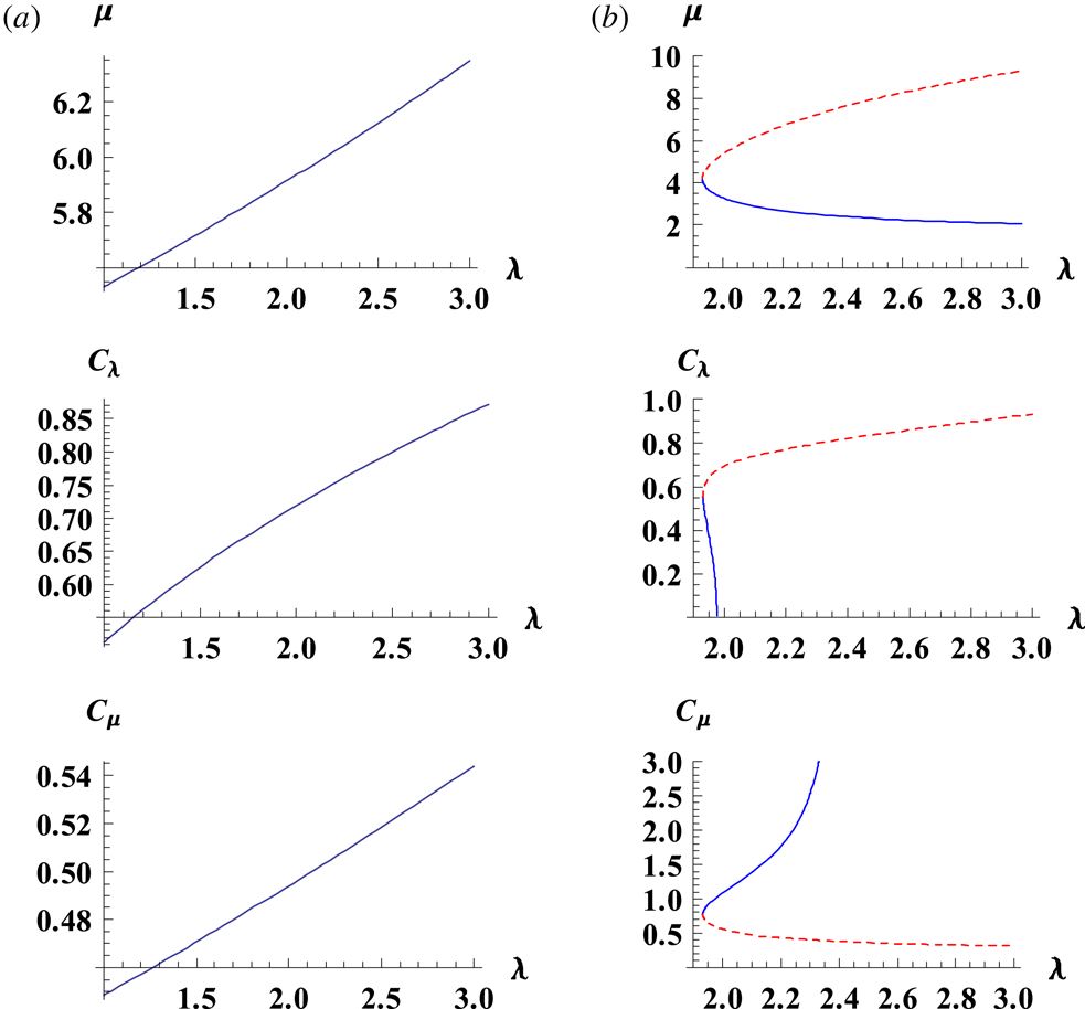
(a) Plots of $\unicode[STIX]{x1D707}$ , $C_{\unicode[STIX]{x1D706}}$ and $C_{\unicode[STIX]{x1D707}}$ versus $\unicode[STIX]{x1D706}$ for the helicity of the ions $h_{i}=25.0$ , no catastrophe. (b) Plots of $\unicode[STIX]{x1D707}$ , $C_{\unicode[STIX]{x1D706}}$ and $C_{\unicode[STIX]{x1D707}}$ versus $\unicode[STIX]{x1D706}$ for $h_{i}=5.0$ . The equilibrium is lost at the critical point $\unicode[STIX]{x1D706}_{\text{crit}}\simeq 1.93$ . The densities of the components $N_{i}=0.88$ , energy of the plasma system $E=5.0$ , helicities of the pair components $h=0.3$ and the Beltrami parameter $b_{+}=0.2$ are taken as constant for both cases.

6 Analysis of double Beltrami equilibrium

To investigate the impact of $N_{i}$ , $h$ , $h_{i}$ and $b_{+}$ on the equilibrium dynamics of an electron, positron and ion plasma, we make use of the equation

(6.1) $$\begin{eqnarray}h_{i}=\frac{(E+\unicode[STIX]{x1D70C}h)}{2}[(\unicode[STIX]{x1D706}+\unicode[STIX]{x1D707})\pm \sqrt{(\unicode[STIX]{x1D706}-\unicode[STIX]{x1D707})^{2}+4}],\end{eqnarray}$$

obtained by using (3.11) and (5.7). Figure 2 shows the characters of $\unicode[STIX]{x1D707}$ , $C_{\unicode[STIX]{x1D706}}$ and $C_{\unicode[STIX]{x1D707}}$ on varying the control parameter $\unicode[STIX]{x1D706}$ keeping all other physical parameters constant. In figure 2(a), plots of $\unicode[STIX]{x1D707}$ , $C_{\unicode[STIX]{x1D706}}$ and $C_{\unicode[STIX]{x1D707}}$ versus $\unicode[STIX]{x1D706}$ are shown for $N_{i}=n_{i}/n_{-}=0.01$ . The other parameters are $E=5.0$ , $h_{i}=5.0$ , $h=0.5$ and $b_{+}=0.2$ . There is no loss of equilibrium when $\unicode[STIX]{x1D706}$ is changed. On the other hand, for the same parameters $E=5.0$ , $h_{i}=5.0$ , $h=0.5$ and $b_{+}=0.2$ , the equilibrium is lost when $N_{i}=0.99$ . 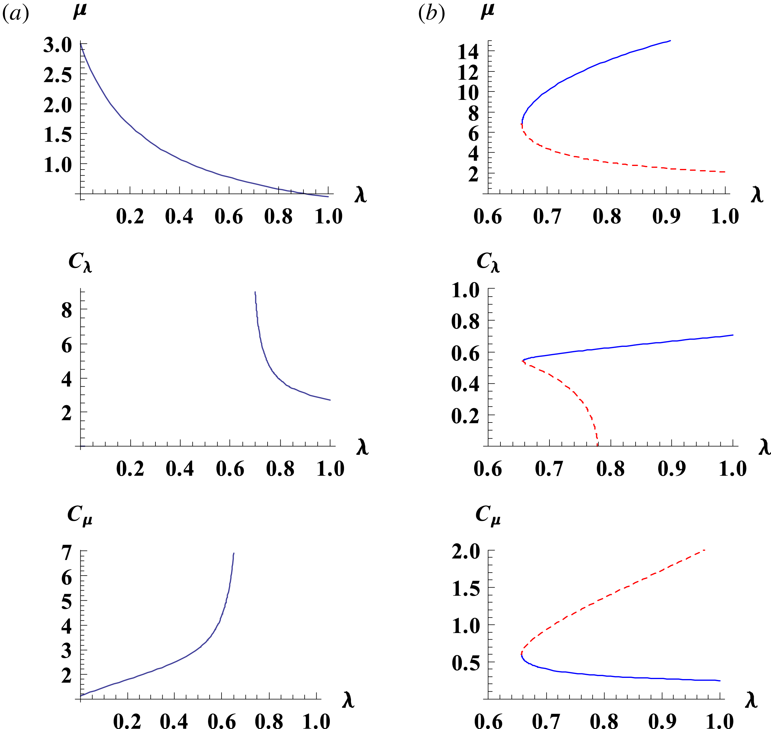It is evident from figure 2(b) that an increase in the number density of the ions as compared to positrons could cause the loss of equilibrium when the scale parameter attains a certain value. The size of the macro-structure increases and equilibrium is lost at a critical point. Figure 3 shows the variation of parameters with respect to the change of scale length $\unicode[STIX]{x1D706}$ for given energy $E=5.0$ , helicity of the ions $h_{i}=5.0$ , densities of the components $N_{i}=0.77$ and Beltrami parameter $b_{+}=0.2$ . It is observed that there is no solution (catastrophic loss of equilibrium) for smaller $h$ – helicities of the pair components of the plasma. Figure 3(a) shows no catastrophe for $h=5.5$ while figure 3(b) shows a loss in equilibrium at $\unicode[STIX]{x1D706}_{\text{crit}}\simeq 0.75$ for $h=0.5$ . The size of the large structure decreases and eruption occurs when the structure reduces to a certain critical value. In contrast to figure 3, keeping $h_{i}$ (helicity of ions) constant in figure 4, we observe that the solution changes drastically by varying $h_{i}$ from $25.0$ to $5.0$ for constant $E=5.0$ , $h=0.3$ , $N_{i}=0.88$ and $b_{+}=0.2$ . In figure 4(a), the system preserves its equilibrium for $h_{i}=25$ while the system faces a fundamentally different situation in figure 4(b) and ceases to be in equilibrium at $\unicode[STIX]{x1D706}_{\text{crit}}\simeq 1.93$ . The sequence of equilibria is lost when the macroscale structure increases to a certain limit. Figure 5 reveals the bifurcation conditions leading to loss of equilibrium for different values of $b_{+}$ (the ratio of magnetic field to positrons flow). Figure 5(a) shows the plots of $\unicode[STIX]{x1D707}$ , $C_{\unicode[STIX]{x1D706}}$ and $C_{\unicode[STIX]{x1D707}}$ versus $\unicode[STIX]{x1D706}$ for $b_{+}=0.01$ . In this case, there is no catastrophe, while figure 5(b) shows the plots of $\unicode[STIX]{x1D707}$ , $C_{\unicode[STIX]{x1D706}}$ and $C_{\unicode[STIX]{x1D707}}$ versus $\unicode[STIX]{x1D706}$ for $b_{+}=0.2$ . The size of the larger structure increases and the equilibrium is lost when the scale parameter reaches a critical value $\unicode[STIX]{x1D706}_{\text{crit}}\simeq 0.656$ . The energy of the plasma system is $E=15.0$ , helicities of pair particles $h=0.5$ , helicity of ions $h_{i}=5.0$ and the densities of the plasma components, $N_{i}=0.77$ , are taken constant for both cases.

Figure 5.

(a) Plots of $\unicode[STIX]{x1D707}$ , $C_{\unicode[STIX]{x1D706}}$ and $C_{\unicode[STIX]{x1D707}}$ versus $\unicode[STIX]{x1D706}$ for the ratio of magnetic field to positron flow $b_{+}=0.01$ , no catastrophe. (b) Plots of $\unicode[STIX]{x1D707}$ , $C_{\unicode[STIX]{x1D706}}$ and $C_{\unicode[STIX]{x1D707}}$ versus $\unicode[STIX]{x1D706}$ for $b_{+}=0.2$ . The equilibrium is lost at the critical point $\unicode[STIX]{x1D706}_{\text{crit}}\simeq 0.656$ . The energy of the plasma system $E=15.0$ , helicities $h=0.5$ and $h_{i}=5.0$ and the densities of the plasma components $N_{i}=0.77$ are taken constant for both cases.

7 Energy and loss of equilibrium

The equilibrium terminates when the system abruptly transforms its state from a DB state to a single Beltrami state. This happens when any one of the amplitudes $C_{\unicode[STIX]{x1D6FC}}$ vanishes and/or the scale parameters become degenerate. Hence, the equilibrium terminates if one of the roots disappears or they become equal.

7.1 Root disappearance

To find the condition for the loss of equilibrium through disappearance of the microscale component of the double Beltrami field, we will determine the extremum, i.e. $\text{d}\unicode[STIX]{x1D706}/\text{d}\unicode[STIX]{x1D707}=0$ for real $\unicode[STIX]{x1D706}$ and $\unicode[STIX]{x1D707}$ ( $\unicode[STIX]{x1D706}$ denotes the macroscale while $\unicode[STIX]{x1D707}$ is the microscale) using (5.8). The use of (5.7), which is equivalent to (5.8), is more suitable for analysis as it describes $b_{i}$ , where $b_{i}$ can be determined fully by the scale parameters $\unicode[STIX]{x1D706}$ and $\unicode[STIX]{x1D707}$ (see (3.11)). Equation (5.7) shows that $b_{i}$ depends on $b_{-}$ , hence we can replace the extremum condition $\text{d}\unicode[STIX]{x1D706}/\text{d}\unicode[STIX]{x1D707}=0$ by $\text{d}\unicode[STIX]{x1D706}/\text{d}b_{-}=0$ . From (3.6), we get,

(7.1) $$\begin{eqnarray}\displaystyle \frac{\text{d}\unicode[STIX]{x1D706}}{\text{d}b_{-}} & = & \displaystyle \frac{\text{d}b_{i}}{\text{d}b_{-}}\left[1+\frac{\left(b_{i}+\unicode[STIX]{x1D70C}\right)}{\sqrt{\left(b_{i}+\unicode[STIX]{x1D70C}\right)^{2}-4}}\right]\nonumber\\ \displaystyle & & \displaystyle -\,\frac{1}{N_{i}b_{-}^{2}}\left[\frac{\left(b_{i}+\unicode[STIX]{x1D70C}\right)}{\sqrt{\left(b_{i}+\unicode[STIX]{x1D70C}\right)^{2}-4}}-1\right]=0,\end{eqnarray}$$

and obtain

(7.2) $$\begin{eqnarray}\frac{\text{d}b_{i}}{\text{d}b_{-}}=\frac{1}{4N_{i}b_{-}^{2}}\left[\sqrt{\left(b_{i}+\unicode[STIX]{x1D70C}\right)^{2}-4}-\left(b_{i}+\unicode[STIX]{x1D70C}\right)\right]^{2}.\end{eqnarray}$$

Using (3.7) in the above equation, we get

(7.3) $$\begin{eqnarray}\frac{\text{d}b_{i}}{\text{d}b_{-}}=\frac{1}{N_{i}b_{-}^{2}}\left(\unicode[STIX]{x1D707}+\unicode[STIX]{x1D70C}\right)^{2}.\end{eqnarray}$$

Another expression for $\text{d}b_{i}/\text{d}b_{-}$ reads as

(7.4) $$\begin{eqnarray}\frac{\text{d}b_{i}}{\text{d}b_{-}}=\frac{hh_{i}}{N_{i}b_{-}^{2}\left(E+\unicode[STIX]{x1D70C}h\right)^{2}},\end{eqnarray}$$

using (5.6) and (3.2). From (7.3) and (7.4), we get

(7.5) $$\begin{eqnarray}hh_{i}=\left[\left(\unicode[STIX]{x1D707}+\unicode[STIX]{x1D70C}\right)\left(E+\unicode[STIX]{x1D70C}h\right)\right]^{2}\geqslant 0,\end{eqnarray}$$

which shows that equilibrium will be lost when the product of the two helicities is positive, otherwise there will be no loss of equilibrium (Ohsaki et al. Reference Ohsaki, Shatashvili, Yoshida and Mahajan2002).

In order to show that the extremum is physically acceptable, we need to evaluate a condition which ensures that all the physical parameters are real at the extremum. In this regard, we eliminate $\unicode[STIX]{x1D707}$ in favour of $b_{i}$ and $b_{-}$ , which results in a quadratic equation in $\unicode[STIX]{x1D70C}$ as expressed below

(7.6) $$\begin{eqnarray}\unicode[STIX]{x1D70C}^{2}\left(h\mp \sqrt{hh_{i}}\right)h+\unicode[STIX]{x1D70C}\left(2h\mp \sqrt{hh_{i}}\right)E+\left(E^{2}+hh_{i}\mp h_{i}\sqrt{hh_{i}}\right)=0.\end{eqnarray}$$

We observed that all the coefficients of the above quadratic equation in $\unicode[STIX]{x1D70C}$ consist of constants of motion ( $h,h_{i},E$ ). The value of $b_{-}$ is real at $\text{d}\unicode[STIX]{x1D706}/\text{d}b_{-}=0$ , if

(7.7) $$\begin{eqnarray}\displaystyle & & \displaystyle \left(2h\mp \sqrt{hh_{i}}\right)^{2}E^{2}-4h\left(h\mp \sqrt{hh_{i}}\right)\left(E^{2}+hh_{i}\mp h_{i}\sqrt{hh_{i}}\right)\nonumber\\ \displaystyle & & \displaystyle \quad =E^{2}-4\left(h\mp \sqrt{hh_{i}}\right)\left(h\mp \sqrt{hh_{i}}\right)\geqslant 0.\end{eqnarray}$$

Simplifying (7.7), we find that extremum will be physical when the following condition holds good

(7.8) $$\begin{eqnarray}E^{2}\geqslant E_{c}^{2}=4\left(h\mp \sqrt{hh_{i}}\right)^{2}.\end{eqnarray}$$

This shows that when the energy $(E)$ of the system is equal to or greater than $E_{c}$ , equilibrium will be terminated.

To find the corresponding value of the control parameter $\unicode[STIX]{x1D706}=\unicode[STIX]{x1D706}_{\text{crit}}$ , we set $\text{d}\unicode[STIX]{x1D706}/\text{d}\unicode[STIX]{x1D707}=0$ , using (3.6) and obtain

(7.9) $$\begin{eqnarray}E\left[1\mp \frac{\left(\unicode[STIX]{x1D706}-\unicode[STIX]{x1D707}\right)}{\sqrt{\left(\unicode[STIX]{x1D706}-\unicode[STIX]{x1D707}\right)^{2}+4}}\right]-2\unicode[STIX]{x1D706}h=0.\end{eqnarray}$$

From (3.2) and (3.3), we have

(7.10) $$\begin{eqnarray}\unicode[STIX]{x1D70C}^{2}+\unicode[STIX]{x1D70C}\left(\unicode[STIX]{x1D706}+\unicode[STIX]{x1D707}\right)+(\unicode[STIX]{x1D706}\unicode[STIX]{x1D707}-1)=0.\end{eqnarray}$$

The solution of the above quadratic equation reads as

(7.11) $$\begin{eqnarray}\unicode[STIX]{x1D70C}=\frac{1}{2}\left[-\left(\unicode[STIX]{x1D706}+\unicode[STIX]{x1D707}\right)\pm \sqrt{\left(\unicode[STIX]{x1D706}-\unicode[STIX]{x1D707}\right)^{2}+4}\right].\end{eqnarray}$$

From (7.9) and (7.11), we obtain

(7.12) $$\begin{eqnarray}E\left(\unicode[STIX]{x1D70C}+\unicode[STIX]{x1D707}\right)-\unicode[STIX]{x1D706}h\left(2\unicode[STIX]{x1D70C}+\unicode[STIX]{x1D706}+\unicode[STIX]{x1D707}\right)=0.\end{eqnarray}$$

This equation can be written as

(7.13) $$\begin{eqnarray}E=\unicode[STIX]{x1D706}h\left[1+\left(\unicode[STIX]{x1D706}+\unicode[STIX]{x1D70C}\right)^{2}\right],\end{eqnarray}$$

using (3.9). This is the value of the energy for which one of the amplitudes $C_{\unicode[STIX]{x1D707}}$ becomes zero (see (5.10)). Initially $C_{\unicode[STIX]{x1D707}}$ is positive and becomes zero at the extremum. As $C_{\unicode[STIX]{x1D707}}=0$ at the extremum, hence one of the Beltrami fields corresponding to $C_{\unicode[STIX]{x1D707}}$ vanishes and, as a result, the DB system reduces to single Beltrami. The extremum thus represents a critical point. When the system goes beyond this extremum point $C_{\unicode[STIX]{x1D707}}$ will become negative so that $C_{\unicode[STIX]{x1D707}}$ becomes imaginary. The critical value of the control parameter $\unicode[STIX]{x1D706}=\unicode[STIX]{x1D706}_{\text{crit}}$ at which transition takes place can be obtained from the simultaneous solution of (5.6) and (7.13). We make use of (3.3) and (5.6) and obtain

(7.14) $$\begin{eqnarray}\tilde{h}_{i}=\left(\unicode[STIX]{x1D706}+\unicode[STIX]{x1D707}+\unicode[STIX]{x1D70C}\right)E-\unicode[STIX]{x1D706}\unicode[STIX]{x1D707}h.\end{eqnarray}$$

Introducing value of $\unicode[STIX]{x1D707}$ from (3.9), the above equation becomes

(7.15) $$\begin{eqnarray}\tilde{h}_{i}=E\unicode[STIX]{x1D706}+\left(E-\unicode[STIX]{x1D706}h\right)\left(\unicode[STIX]{x1D706}+\unicode[STIX]{x1D70C}\right)^{-1}+\unicode[STIX]{x1D706}h\unicode[STIX]{x1D70C}.\end{eqnarray}$$

The above equation can be written as follows on using (7.13)

(7.16) $$\begin{eqnarray}\left(\unicode[STIX]{x1D706}+\unicode[STIX]{x1D70C}\right)[\tilde{h}_{i}-\unicode[STIX]{x1D706}\left(E-\unicode[STIX]{x1D706}h\right)]=2\left(E-\unicode[STIX]{x1D706}h\right).\end{eqnarray}$$

Using (7.13), the above equation becomes

(7.17) $$\begin{eqnarray}[\tilde{h}_{i}-Q]^{2}=4hQ,\end{eqnarray}$$

where

(7.18) $$\begin{eqnarray}Q=\unicode[STIX]{x1D706}\left(E-\unicode[STIX]{x1D706}h\right).\end{eqnarray}$$

Putting $\tilde{h}_{i}=h_{i}-h$ , into (7.17), we get

(7.19) $$\begin{eqnarray}Q=\left(\sqrt{h}\pm \sqrt{h_{i}}\right)^{2}.\end{eqnarray}$$

From (7.18) and (7.19), using (7.8) and taking $\unicode[STIX]{x1D706}=\unicode[STIX]{x1D706}_{\text{crit}}$ , we get

(7.20) $$\begin{eqnarray}\unicode[STIX]{x1D706}_{\text{crit}}=\frac{1}{2h}\left[E\pm \sqrt{E^{2}-E_{c}^{2}}\right].\end{eqnarray}$$

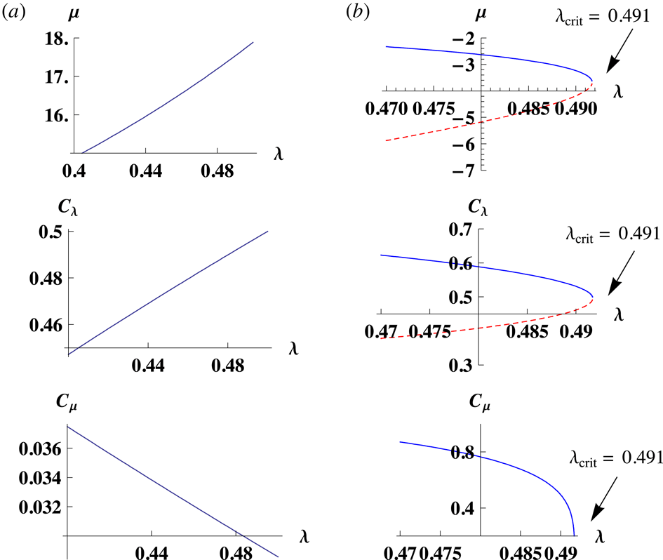
In order to show the catastrophic loss of equilibrium, the plots of $\unicode[STIX]{x1D707}$ and $C_{\unicode[STIX]{x1D6FC}}$ as functions of $\unicode[STIX]{x1D706}$ are displayed in figure 6 for given values of the invariants $h,h_{i},E$ and the densities of the plasma components. The equilibrium exists until $\unicode[STIX]{x1D707}$ and $C_{\unicode[STIX]{x1D6FC}}$ remain real, otherwise the equilibrium will be lost. Figure 6 shows the two sets of plots for two distinct values of energy while all other parameters are kept constant. The values of the parameters are taken as $h=0.5$ , $h_{i}=5.0$ and $n_{i}=n_{+}=0.5n_{-}$ . We have considered a constant density of the plasma constituents and this is an essential feature of this model which is missing in Hall MHD (Ohsaki et al. Reference Ohsaki, Shatashvili, Yoshida and Mahajan2001, Reference Ohsaki, Shatashvili, Yoshida and Mahajan2002). The factor of density appears naturally in the present system to describe the self-organized structures as the scale parameters $\unicode[STIX]{x1D706}$ and $\unicode[STIX]{x1D707}$ depend on the number densities of the species. It is observed that energy plays a key role in determining the loss of equilibrium. There exists a critical value of energy $E_{c}$ which plays a key role in defining the fate of the system. If the energy of the system is less than that of the critical value, the system remains in its state of equilibrium, but if the energy becomes equal to or exceeds the critical value $E_{c}$ , the system faces a catastrophic loss of equilibrium. In figure 6(a), the value of energy is taken to be $0.5$ which is less than the critical value of energy $E_{c}\simeq 2.16$ . In this case, the physical parameters $\unicode[STIX]{x1D707}$ and $C_{\unicode[STIX]{x1D6FC}}$ change smoothly and continuously by varying the control parameter $\unicode[STIX]{x1D706}$ . As $\unicode[STIX]{x1D707}$ and $C_{\unicode[STIX]{x1D6FC}}$ remain real, we observe equilibrium and there is no qualitative change and hence no catastrophe. On the other hand, in figure 6(b), the energy is taken to be 5, which is greater than the critical value. The parameters $\unicode[STIX]{x1D707}$ and $C_{\unicode[STIX]{x1D6FC}}$ do not remain real and become complex, as shown by the dotted lines. At this stage, the value of $\unicode[STIX]{x1D706}$ reaches a critical value $\unicode[STIX]{x1D706}_{\text{crit}}$ where the size of this macroscale structure reduces to such an extent that one of the amplitudes $C_{\unicode[STIX]{x1D706}}$ becomes complex. Consequently, the sequence of equilibrium is lost and the system is no longer in equilibrium.

Figure 6.

(a) Plots of $\unicode[STIX]{x1D707}$ , $C_{\unicode[STIX]{x1D706}}$ and $C_{\unicode[STIX]{x1D707}}$ versus $\unicode[STIX]{x1D706}$ for $E=0.5<E_{c}\simeq 2.16$ , the critical energy; no catastrophe. (b) Plots of $\unicode[STIX]{x1D707}$ , $C_{\unicode[STIX]{x1D706}}$ and $C_{\unicode[STIX]{x1D707}}$ versus $\unicode[STIX]{x1D706}$ for $E=5>E_{c}\simeq 2.16$ . The equilibrium is lost at the critical point $\unicode[STIX]{x1D706}_{\text{crit}}\simeq 0.491$ . The densities of the plasma components are taken as $n_{i}=n_{+}=0.5n_{-}$ .

Figure 7.

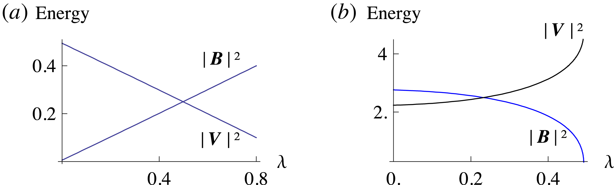
(a) Plots of magnetic and flow energies versus $\unicode[STIX]{x1D706}$ for $E=0.5<E_{c}\simeq 2.16$ , the critical energy; no catastrophe. (b) Plots of magnetic and flow energies versus $\unicode[STIX]{x1D706}$ for $E=5>E_{c}\simeq 2.16$ . The equilibrium is lost at the critical point $\unicode[STIX]{x1D706}_{\text{crit}}\simeq 0.491$ . The densities of the plasma components are taken as $n_{i}=n_{+}=0.5n_{-}$ .

For the same set of parameters as used in figure 6, the characters of the magnetic and flow energies are depicted in figure 7. The flow energy decreases and magnetic energy increases when the control parameter is increased, as shown in figure 7(a). The system energy $(E=0.5)$ is less than the critical value $(E_{c}\simeq 2.16)$ and the equilibrium is preserved. Figure 7(b) shows that magnetic energy decreases while the flow energy increases as the control parameters are increased slowly. Almost all the magnetic energy is converted to flow energy at $\unicode[STIX]{x1D706}_{\text{crit}}$ . 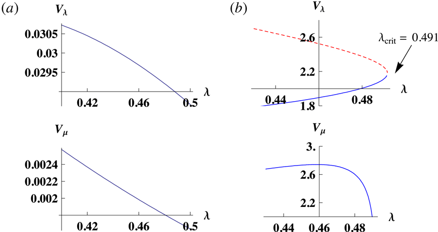In figure 7(b), it is observed that $V^{2}/B^{2}$ approaches infinity at $\unicode[STIX]{x1D706}_{\text{crit}}=0.491$ , whereas, on the other hand, when there is no catastrophe $V^{2}=B^{2}=1$ , that is $\boldsymbol{V}^{2}=\boldsymbol{B}^{2}$ at $\unicode[STIX]{x1D706}_{\text{crit}}=0.491$ as shown in figure 7(a). This shows a true manifestation of catastrophe as the magnetic energy is transformed to flow kinetic energy. Figure 8 displays the profiles of the flows ( $V_{\unicode[STIX]{x1D706}}$ and $V_{\unicode[STIX]{x1D707}}$ ) associated with both the scale parameters $\unicode[STIX]{x1D706}$ and $\unicode[STIX]{x1D707}$ . Figure 8(a) shows the velocities when there is no catastrophe. It is evident that the flow velocities of the macroscale component $(V_{\unicode[STIX]{x1D706}})$ and microscale component $(V_{\unicode[STIX]{x1D707}})$ both decrease on increasing the control parameter $(\unicode[STIX]{x1D706})$ . Figure 8(b) shows the same profiles for energy $E>E_{c}\simeq 2.16$ . In this scenario, the system is bound to face catastrophe when the control parameter reaches its critical value. It can be observed from figure 8(b) that the flow of large scale structures increases while the flow of smaller scales structure reduces. Thus the flow energy of the microscale component is transferred to the macroscale component and at $\unicode[STIX]{x1D706}_{\text{crit}}$ , the flow energy attains such a value that it is hard for the system to stay in equilibrium and consequently the catastrophic loss of equilibrium occurs. At this point, the flow energy becomes very high while the magnetic energy diminishes and becomes zero. The system thus transforms to a single Beltrami state which appears when the magnetic energy of the system decays to its ground state (Taylor Reference Taylor1974, Reference Taylor1986; Yoshida, Mahajan & Ohsaki Reference Yoshida, Mahajan and Ohsaki2004).

Figure 8.

(a) Plots of $V_{\unicode[STIX]{x1D706}}$ and $V_{\unicode[STIX]{x1D707}}$ versus $\unicode[STIX]{x1D706}$ for $E=0.5<E_{c}\simeq 2.16$ , the critical energy; no catastrophe. (b) Plots of $V_{\unicode[STIX]{x1D706}}$ and $V_{\unicode[STIX]{x1D707}}$ versus $\unicode[STIX]{x1D706}$ for $E=5>E_{c}\simeq 2.16$ . The equilibrium is lost at the critical point $\unicode[STIX]{x1D706}_{\text{crit}}\simeq 0.491$ . The densities of the plasma components are taken as $n_{i}=n_{+}=0.5n_{-}$ .

7.2 Root degeneracy

The equilibrium may terminate in the slowly evolving DB states when the two constituent states change themselves so that they become degenerate. This path to termination of equilibrium is fundamentally different from that of the root disappearance mode where the amplitudes of one of the original states vanishes and consequently the DB states relaxes to a single Beltrami state. The same phenomenon occurs when both of the original states coalesce to a single independent state, that is, the two scale parameters become degenerate. In this situation, the critical point acts as a boundary between the real and a pair of complex conjugate roots (scale parameters) of the DB states. In this way the critical point behaves as a boundary between the paramagnetic and diamagnetic structures. The conditions for the loss of equilibrium through degeneracy of the roots are satisfied when the parameters of the system make the $\unicode[STIX]{x1D706}(\unicode[STIX]{x1D707})$ curve intersect the $\unicode[STIX]{x1D706}=\unicode[STIX]{x1D707}$ line for real $\unicode[STIX]{x1D706}$ at the critical point, there is no scale separation. This shows that the parametric space for which the roots become degenerate is entirely different from the parametric space where one of the roots disappears. Hence, the field structures pertaining to the degeneracy of roots will be quite different. Using $\unicode[STIX]{x1D706}=\unicode[STIX]{x1D707}=\unicode[STIX]{x1D706}_{0}$ , we obtain from (3.11)

(7.21) $$\begin{eqnarray}b_{i}=\unicode[STIX]{x1D706}_{0}\pm 1.\end{eqnarray}$$

Using the above value of $b_{i}$ in (5.6), we obtain

(7.22) $$\begin{eqnarray}\tilde{h}_{i}=E\left(\unicode[STIX]{x1D706}_{0}\pm 1\right)-\unicode[STIX]{x1D706}_{0}^{2}h.\end{eqnarray}$$

Solving above equation, we obtain

(7.23) $$\begin{eqnarray}\unicode[STIX]{x1D706}_{0}=\frac{1}{2h}\left[E\pm \sqrt{E^{2}-4h(\tilde{h}_{i}\mp E)}\right].\end{eqnarray}$$

The condition for the loss of equilibrium when the roots become degenerate reads as

(7.24a,b ) $$\begin{eqnarray}E^{2}>E_{0}^{2},\quad E_{0}^{2}=4\left(h\mp \sqrt{hh_{i}}\right)^{2}.\end{eqnarray}$$

Elimination of $E$ from (7.13) and (5.9) gives

(7.25) $$\begin{eqnarray}C_{\unicode[STIX]{x1D706}}^{2}=\unicode[STIX]{x1D706}h.\end{eqnarray}$$

Putting $\unicode[STIX]{x1D706}=\unicode[STIX]{x1D707}$ in (7.13), we get

(7.26) $$\begin{eqnarray}E=\unicode[STIX]{x1D707}h\left(\left(\unicode[STIX]{x1D707}+\unicode[STIX]{x1D70C}\right)^{2}+1\right).\end{eqnarray}$$

Putting the above value of $E$ into (5.10) we get

(7.27) $$\begin{eqnarray}C_{\unicode[STIX]{x1D707}}^{2}=\unicode[STIX]{x1D706}h.\end{eqnarray}$$

Figure 9.

Plots for the catastrophe conditions through coalescence of the roots. (a) $E=1.5<E_{c}\simeq 2.16$ , the critical energy; no catastrophe. (b) $E=5>E_{c}\simeq 2.16$ , with $h=0.5$ and $h_{i}=5$ in both cases.

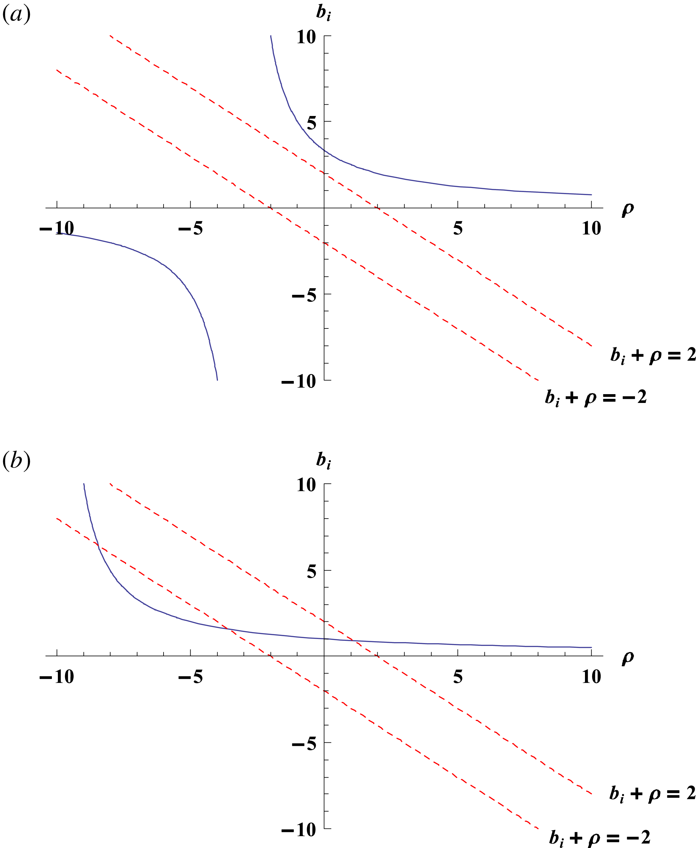
Equations (7.25) and (7.27) show that both the amplitudes become equal when the roots coalesce. Figure 9 shows graphs of $b_{i}$ versus $\unicode[STIX]{x1D70C}$ for $h=0.5$ and $h_{i}=5$ for both the catastrophe-free and catastrophe-prone energies. The dashed lines in both the graphs show the values of $b_{i}$ and $\unicode[STIX]{x1D70C}$ when both $\unicode[STIX]{x1D706}$ and $\unicode[STIX]{x1D707}$ are equal. The solid curves are drawn using (5.7). In figure 9(a), the energy taken is less than the critical energy. We find no crossing of the curves and the dashed lines, which shows that there will be no catastrophe when $\unicode[STIX]{x1D706}$ and $\unicode[STIX]{x1D707}$ are equal. On the other hand, the dashed lines and curves cross each other for $E=5$ which is greater than $E_{c}\simeq 2.16$ as shown in figure 9(b). In this case, the equilibrium will be lost.

In the present study, a constant density ratio of plasma particles is considered. The system could be transformed from para to diamagnetic states on varying the density ratio of the plasma components (Gondal et al. Reference Gondal, Iqbal, Khosa and Murtaza2017). The present study could be helpful in improving our knowledge about a variety of eruptive events occurring in multi-component astrophysical space plasmas.

8 Summary

The steady state equilibrium of an electron, positron and ion plasma can be expressed by three simultaneous Beltrami conditions showing the alignment of the fields and flows. Solving these equations, we obtain a double curl Beltrami equation. The double Beltrami field, being the sum of two Beltrami fields, is completely specified by two eigenvalues (scale parameters) and two amplitudes. The equations showing the relationships of the scale parameters, amplitudes and conserved physical quantities are developed to investigate the impact of densities, helicities and the ratio of field to positron flow on the loss of equilibrium by slowly varying the control parameter (one of the scale parameters). Keeping all the physical parameters constant, it is found that when the density of the ions is very small as compared to the positron density, the system remains in equilibrium when the control parameter is changed slowly. On the other hand, for a higher density of ions, we observe that the size of the macroscale structure increases and a loss of equilibrium occurs at a particular value of the control parameter. Moreover, for higher values of the helicities of the inertialess components, there is no catastrophic loss of equilibrium. However, for the lower helicities, the equilibrium is lost catastrophically when the macroscale shrinks to a critical value. Similar behaviour is observed for the ion helicity. It is worth noting that the size of the macroscale structure increases and leads to a loss of equilibrium for a smaller ion helicity. It is also found that positron flows effect the system dynamics and can cause loss of equilibrium.

The conditions for the loss of equilibrium are also derived. It is found that the energy of the system determines whether the system is likely to lose equilibrium or not. There exists a critical energy value which depends on the helicities. If the energy of the system is less than or equal to this critical energy, the system preserves its equilibrium for given helicities and scale parameters. On the other hand, when the system’s energy is greater than the critical value, the equilibrium will be lost at a particular value of the control parameter. The relation between the critical value of the control parameter and critical energy of the system is also derived. It is also observed that when equilibrium is lost, the magnetic energy becomes zero and most of the energy is converted to flow kinetic energy. This conversion of magnetic energy to flow energy suggests that the phenomenon is a manifestation of an eruptive event. The present work is useful to understand a variety of eruptive events taking place in space and astrophysical plasmas.