Implications
Sheep production environments can vary in terms of resources and management schemes. With such variation there is a risk that genotype by environment interactions (G×E) may exist, potentially reducing the efficiency of index selection and economic performance of flocks. By grouping flocks into similar environment types, this study found evidence of G×E in a sample of UK Charollais flocks when the response of genotypes to different environments was assessed. The identification of genotypes best suited to certain environments, or alternatively genotypes that perform consistently across environments, will allow producers to use G×E to their advantage, thus reducing inefficiency in performance.
Introduction
Genetic evaluations currently carried out for livestock use best linear unbiased prediction (BLUP) technology (Henderson, Reference Henderson1975). In sheep breeding, providing there are suitable levels of genetic linkage between flocks, BLUP allows estimated breeding values (EBVs) to be expressed relative to a common base, from which direct comparisons can be made across flocks. However, a problem that farmers can encounter is that having selected to use an individual animal based on their predicted performance, they obtain somewhat unexpected and inconsistent results when they are used in another location (Cienfuegos-Rivas et al., Reference Cienfuegos-Rivas, Oltenacu, Blake, Schwager, Castillo-Juarez and Ruiz1999).
The association between environment and the phenotypic expression of a genotype constitute a genotype by environment interaction (G×E), which can occur when genotypes respond differently to changes in the environment (Falconer and MacKay, Reference Falconer and MacKay1996). G×E studies in sheep are limited in number, particularly when compared with the dairy industry, perhaps due to the lack of globalisation within the industry, the use of locally adapted breeds in many areas and the often extensive nature of the production systems. Each flock has its own unique set of resources and management schemes. To investigate G×E, it may be valuable to classify individual flocks into different groups, based on variables related to climatic conditions, nutrition and overall flock management. One option available is to consider farm typologies, which use multivariate statistical methods to identify homogeneous groups of farms (Köbrich et al., Reference Köbrich, Rehman and Khan2003), allowing clusters, or groups, to be defined from large data sets that include a number of uncorrelated variables. In the dairy industry, Weigel and Rekaya (Reference Weigel and Rekaya2000), Zwald et al. (Reference Zwald, Weigel, Fikse and Rekaya2003) and Huquet et al. (Reference Huquet, Leclecr and Ducrocq2012a) have used cluster analyses in order to group countries, or individual herds. Similar methods have also been used by Neser et al. (Reference Neser, Erasmus and Scholtz2008) and Espasandin et al. (Reference Espasandin, Urioste, Naya and Alencar2013) when investigating G×E in beef cattle systems.
The purpose of this study was, initially, to develop a terminal sire sheep farm typology, exploring the differences and similarities of farms that performance-record their sheep as part of the Signet Sheepbreeder programme (www.signetfbc.co.uk). Then, using the clusters identified, the presence of G×E, for traits important for the genetic improvement of terminal sire lambs, was investigated using data available for Charollais lambs as a case-study.
Material and methods
Farm questionnaire
A questionnaire was developed, which adhered to the principles of Fowler (Reference Fowler2002), and was sent to all 515 members of the Signet Sheepbreeder programme. The questions posed covered aspects such as the farm location and land cover; sheep numbers and breed; the management of the flock at mating, ultrasound pregnancy scanning, lambing, weaning and post weaning; grazing and feeding throughout the year (Grazing options provided were; hill/rough grazing; in-bye/improved pasture; hay/silage fields; any other crop field. Feeding options provided were; feed blocks; hay; silage; concentrate feed); the use of vitamins and mineral supplements (as well as other health treatments) and labour use. The format of the questions varied, with some requiring a numerical answer (e.g. ewe numbers, ram to ewe ratios at mating, land areas); some a tick-box answer (e.g. the months concentrate feed was available, grazing locations throughout the year); some were scaled questions (e.g. grade the quality of grazing available between weaning and mating on a scale of 1 (poor quality) to 5 (high quality)) and some questions could be answered yes or no (e.g. organic or nonorganic, has any chemical resistance been identified on your farm).
The questionnaire attempted to characterise the specific management of each recorded sheep flock, relevant to the production data, and disregarded information on other enterprises on the farm. Where more than one breed was performance recorded on the same farm, respondents were asked to select one breed and answer the remaining questions based on the management of that breed only. A total of 200 questionnaires were returned, from a possible 515, achieving a 39% response rate. The questionnaires returned provided information for 28 different breeds, with the main terminal sire breeds (Charollais, Texel and Suffolk) providing 45% of the questionnaire respondents. Due to the high percentage of terminal sire breeders replying, the analysis concentrated on these breeds only. A number of questionnaires returned (n=11) were not complete, therefore 79 questionnaires from terminal sire flocks, across the United Kingdom, were used in the final analysis (consisting of 21 Charollais flocks, 18 Suffolk flocks and 40 Texel flocks). Terminal sire breeders record their animals for genetic analysis using the Terminal Sire Index, which is used to help select individuals with increased lean meat yield in the carcass, but without increased levels of fatness (Simm and Dingwall, Reference Simm and Dingwall1989; Macfarlane and Simm, Reference Macfarlane and Simm2007).
Weather and lambing data
The farm postcode was used to identify a longitude and latitude value for each farm location, using Bing Maps (http://www.bing.com/maps/), as well as regional monthly rainfall (mm), average temperature (°C) and hours of sunshine (http://www.metoffice.gov.uk/climate/ruk/datasets/). Means for each season were calculated over a 5-year period (2005 to 2009), with the seasons being classified as: winter (December to February), spring (March to May), summer (June to August) and autumn (September to November). Lambing dates were available from Signet, via the Basco Database (http://www.egenes.co.uk/bascosearchsheep/). The percentage of lamb births recorded during winter and spring, for each flock between the 2005 and 2009 breeding seasons, were used in the analysis.
Typology analysis
The analysis was carried out by a series of steps using Genstat (11th edition, VSN International Ltd, 2008). Where pairs of variables were found to be highly correlated (r⩾0.90 or ⩽−0.90), one variable from each pair was removed. Variables that did not show any variation were also removed, as they provided little assistance to the development of the clusters (Köbrich et al., Reference Köbrich, Rehman and Khan2003). A similarity matrix was created between each variable included in the analysis, using simple matching and Euclidean methods for the discrete and quantitative variables respectively, as described by Gower (Reference Gower1971). The similarity coefficients calculated ranged from zero (completely different) to one (absolutely identical). These data were then used in a subsequent principal coordinate (PCO) analysis. A non-hierarchical cluster analysis was then carried out on the PCO scores, using the between-group sum of squares criterion, in order to maximise Euclidean distance between groups. To assess the overall differences between the identified clusters, a one-way ANOVA was used for the quantitative variables, while a Kruskal–Wallis analysis was used for the discrete variables. In order to establish significant differences between each cluster, LSD tests and Bonferroni corrected Mann–Whitney U tests were used as post-hoc tests for the ANOVA and Kruskal–Wallis analyses, respectively.
Genetic analyses
Performance records for the Charollais flocks that responded to the questionnaire were then further analysed to determine if G×E was evident between the different clusters. The traits studied were 21-week weight (21WT), ultrasound muscle depth (UMD) and log transformed ultrasound fat depth (LogUFD), all of which are measured once in the lifetime of the lamb, according to Signet Sheepbreeder protocol (www.signetfbc.co.uk). UFD was transformed to approximate normality. The average age of the lambs at 21WT was 149 days (range 85 to 215 days). Ultrasonic fat depth and UMD measurements were taken at the 3rd lumbar on the same day as the 21WT. The pedigree file used in the analyses contained sire and dam information for a total of 161 431 animals. Heritability estimates for each trait were estimated using univariate analyses in ASReml (Gilmour et al., Reference Gilmour, Cullis, Welham and Thompson2001) across all, as well as within, each cluster identified. Random effects in the models included a direct genetic effect (animal), maternal genetic effect (dam) and the common environment effect (c 2 ), that is variation caused by the environment which the rearing ewe (either genetic dam, embryo transfer recipient dam or foster dam) provided for the lamb. The inclusion of all three random effects significantly improved the models when tested for each trait using the data set including all farms. All three effects were further retained for each individual cluster analysis in order to maintain consistency.
All biologically sensible effects and interactions were tested in order to find an appropriate fixed effects model, resulting in the following model being fitted for each trait:
 $$\eqalignno{ {\rm Trait}=\,& {\rm mean}{\plus}{\rm sex}{\plus}{\rm age}{\plus}{\rm litter size}{\plus}{\rm birth year}{\plus}{\rm birth flock}\cr {\plus}{\rm rearing dam age}{\plus} \left( {{\rm sex}{\times}{\rm age}} \right){\plus}\left( {{\rm sex}{\times}{\rm litter size}} \right)\cr & {\plus}{\rm animal}{\plus}{\rm dam}{\plus}c^{2} {\plus}{\rm error} $$
Age was the age of the lamb (in days) at measurement, treated as a covariate. Rearing dam age, however, was a fixed effect measured in years (14 levels: 1 to 14 years old). Other factors included lamb birth year (21 levels: 1990 to 2010) and sex (2 levels: male and female) and litter size at birth (4 levels: 1 to 4 and above).
To investigate the presence of G×E, genetic correlations for the same traits across clusters were estimated by a series of bivariate analyses in ASReml, similar to the method proposed by Falconer (Reference Falconer1952). The models used were similar to those used for the univariate analyses. However, the random effects fitted for bivariate UMD model were reduced to include only the direct genetic effect (animal) and the common environment effect (c 2 ) as the addition of the maternal genetic effect did not significantly improve the model. The estimated correlations were then tested using a log-likelihood ratio test (LR). For each trait, the log-likelihood for the original bivariate analysis (logL0) was taken from an analysis where all parameters were estimated. The genetic correlation was then fixed close to unity (0.999) and the log-likelihood recalculated (logL1). This analysis required one less parameter to be estimated than the full analysis. The test statistic, LR=2(logL0−logL1), therefore had a chi-squared distribution with one degree of freedom, from which any significant genotype by cluster difference, although providing a conservative cut-off point, could be determined (Morrell, Reference Morrell1998). Spearman’s rank and Pearson’s correlation analyses were also calculated using the EBVs estimated using the bivariate analyses, for sires with 10 or more offspring in at least two of the different cluster groups.
Results
Typology analysis
The data gathered from the questionnaires, as well as the weather and lambing season information, illustrated a wide range of different farming systems and locations. Farm size ranged from 3 to 10 930 ha (average 272 ha), representing small lowland farms to large hill farming estates. Total recorded flock size ranged from 12 to over 400 ewes. When asked to classify their farm, three respondents selected hill-type system, 21 selected upland and 55 selected lowland. Some farms performance recorded all of their ewes, while others only recorded a proportion. The most commonly used grazing type throughout the year was in-bye/improved grazing, closely followed by the hay/silage field type grazing. In terms of labour, 49% of respondents spent less than a quarter of their time working with the recorded ewe flock.
PCO analysis
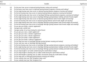
Overall, the PCO analysis used 146 variables (117 discrete and 29 quantitative), including questionnaire answers, weather data and lambing dates. Although 10 dimensions explained 100% of the variation, only the initial six were subsequently retained since each additional dimension did little to distinguish the clusters and the associated variables proved statistically non-significant. The six dimensions retained explained 73% of the total variation, a threshold deemed suitable by Gasper et al. (Reference Gaspar, Escribano, Mesias, Rodriguez de Ledesma and Pulido2008). The variables with correlation coefficients ⩾0.5, or ⩽−0.5, with any of the six dimensions were investigated further for interpretation purposes (Table 1).
Variables and correlation coefficients (r) used to characterise PCO dimension 1 to 6

PCO=principal coordinate; ns=not significant (P>0.05).
Overall differences between clusters assessed by ANOVA and Kruskal–Wallis for quantitative and discrete variables respectively.
***, ** and *Significantly different (P<0.001), (P<0.01), (P<0.05), respectively.
PCO dimension 1: seasonal grazing
Dimension 1, which explained 20% of the variation, was predominantly related to the use of in-bye/improved and hay/silage types of grazing. The in-bye/improved grazing variables identified in this dimension were related to the ewes grazing between pregnancy scanning and lambing, as well as the single- and multiple-rearing ewes between the 8-week lamb weight and weaning. The hay/silage field variables were also related to the period between the 8-week lamb weight and weaning for single- and multiple-rearing ewes, as well as for the single-rearing ewes between pregnancy scanning and the 8-week lamb weight. The use of lamb vitamin supplements was also included in this dimension.
PCO dimension 2: weather and vitamin/mineral supplementation
Dimension 2 was influenced by sunshine hours and rainfall and explained 14% of the variation. The supplementation of cobalt and selenium (both ewes and lambs) and vitamins (ewes) were also associated with this dimension.
PCO dimension 3: the use of hay/silage field grazing
Dimension 3, which explained 12% of the variation, was solely related to the grazing of hay/silage fields: between weaning and mating; during mating; for multiple-rearing ewes between pregnancy scanning and the 8-week lamb weight; and for single-rearing ewes between pregnancy scanning and lambing.
PCO dimension 4: ram management
Dimension 4 was influenced by ram management (predominantly ‘bought-in’ animals) during the month before mating, including where rams/ram lambs were kept (housed or outside) and whether or not concentrate feeding was provided. Overall, 10% of the variation was explained by this dimension.
PCO dimensions 5 and 6: use of hill/rough type grazing and ectoparasite treatments
Dimension 5 (9% of variation) was associated with just one variable, the use of hill/rough grazing by the ewes between weaning and mating, whereas dimension 6 (8% of variation) was influenced by the control of ectoparasites, such as sheep scab and lice.
Non-hierarchical cluster analysis
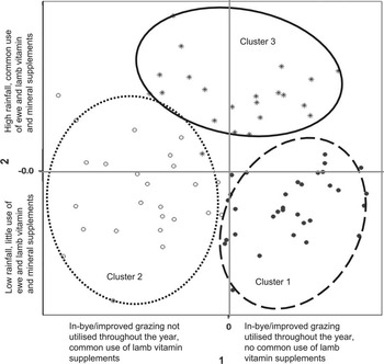
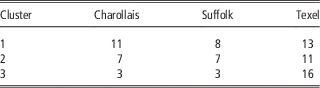
Overall, it was possible to identify three homogenous clusters of farm environments (Figure 1). Of the 79 farms, 32 were in the first cluster, 25 in the second and 22 in the third. All three terminal sire breeds were represented in each of the groups (Table 2). Comparison of PCO dimension 1 with PCO dimension 2 clearly showed that the farm clusters were distinct, but appeared less so when other pairs of dimensions were compared (Figure 1). The ANOVA and Kruskal–Wallis on the descriptive variables, highlighted by each dimension, supported this distinction since the statistical significance dropped in line with the percentage variance.
Positioning of farms according to the scores obtained for principle dimensions 1 and 2.

Number of flocks within each cluster

Cluster 1
Cluster 1 flocks predominantly used in-bye/improved grazing throughout the year, significantly more (P<0.05) than flocks in Cluster 2 (Supplementary Table S1). Few gave vitamin or mineral supplements to ewes or lambs, indeed significantly fewer (P<0.05) when compared with Cluster 2 and Cluster 3 for all, with the exceptions of copper (Cluster 2 and Cluster 3) and cobalt and selenium (Cluster 2), (Supplementary Table S2). Other characteristics of Cluster 1 flocks (Supplementary Table S3) included an average farm size of 128 ha, an average flock size of 88.3 recorded ewes and an average of 249.4 ewes in total. Rainfall averages, throughout the year, were significantly lower (P<0.001) than those of Cluster 2 and Cluster 3. The average hours of sunshine, during the summer, autumn and winter months, were significantly higher (P<0.05) than in Cluster 3. Average temperatures for Cluster 1 flocks were significantly higher (P<0.05) than Cluster 3 during the spring, summer and autumn months. The average number of days that the rams were with the ewes during mating was 48.1, significantly higher (P<0.05) than those in Cluster 2 (33.4 days). On average, 59.8% of lambs born into these flocks were born during the winter months (December to February). Supplementary feed blocks were, on average, used for 1.2 months a year, which was significantly lower (P<0.05) than in Cluster 2 (3.7 months). The average number of weeks that the lambs had access to concentrate feed before weaning was 6.5. Only 44% of flocks regularly treated for liver fluke, which was significantly lower (P<0.001) when compared with 91% in Cluster 3.
Cluster 2
In Cluster 2, an increased proportion of flocks used hay/silage field grazing between pregnancy scanning and weaning, significantly different (P<0.05) when compared with Cluster 1 (Supplementary Table S1). There was also a significant difference between pregnancy scanning and lambing (P<0.05) when compared with Cluster 3 (Supplementary Table 1). The data presented in Supplementary Table S3 shows that farms in this cluster had significantly less (P<0.05) in-bye/improved grazing (26.1% as a proportion of their farm) compared with those in Cluster 3 (54.5%). The average farm size in Cluster 2 was 543.8 ha, but this was not significantly different (P>0.05) to either Cluster 1 or Cluster 3, due to a high standard deviation. The average number of recorded ewes per farm was 75.4, with an average total ewe flock of 587.7 ewes. Flocks in this cluster, on average, mated 36.6 ewes via AI, a significantly higher number (P<0.05) when compared with an average of just 7 in Cluster 3. The average number of days that the ewes were with a ram was 33.4, which was significantly lower (P<0.05) than Cluster 1. The average percentage of lamb births in winter was 67% and lambs had access to concentrate feed, on average, 8.1 weeks before weaning (Supplementary Table S3).
Cluster 3
The third cluster, similar to Cluster 1, also relied heavily on improved/in-bye grazing and less on hay/silage field grazing. Indeed, on average, the farms within this cluster had over 50% of their farm made up of improved grazing, a significantly higher proportion (P<0.05) than Cluster 2. The average farm size in Cluster 3 was 173.6 ha, the average number of recorded ewes on each farm was 87, with an average total ewe flock of 578.3 ewes. The flocks in this cluster were associated with significantly higher (P<0.001) rainfall averages, throughout the year, when compared with both Cluster 1 and Cluster 2. This may be related to the fact that a significantly high proportion (P<0.05) of flocks within this cluster (91%), compared with those in Cluster 1 (44%), routinely treated their animals for liver fluke, a problem commonly associated with areas of higher rainfall. Flocks in Cluster 3 also experienced significantly fewer hours of sunshine (P<0.05) during the summer, autumn and winter months when compared with flocks in Cluster 1. Average temperatures were significantly lower (P<0.05) than those for Cluster 1 during the spring, summer and autumn months (Supplementary Table S3). A high proportion also provided their ewes and lambs with cobalt, selenium and vitamin supplements (Supplementary Table S2), which was significantly higher (P<0.05) than flocks in Cluster 1. Flocks in this cluster had a higher average of ewes mated naturally, (75.8) and a significantly lower (P<0.05) average number of ewes mated via artificial insemination (AI) (7.1), when compared with Cluster 2. The average percentage of lamb births registered during the spring months was 52.1% and was higher than both Cluster 1 and Cluster 2 flocks (33.9% and 28.8%, respectively). Finally, the lambs, on average, had access to creep feeding 5.4 weeks before weaning, less than both Cluster 1 and 2 (6.5 and 8.1 weeks, respectively; Supplementary Table S3).
Genetic analyses
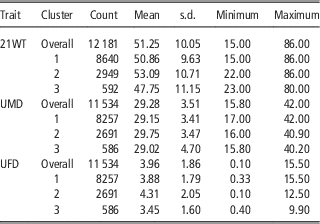
Performance data were available for 18 of the 21 responding Charollais flocks and included animals sired by a total of 515 different sires, between 1990 and 2010. Data were unavailable for three newly recorded flocks (two allocated to Cluster 1 and one allocated to Cluster 2), while an additional flock from Cluster 2 had no ultrasound data. Of the 515 sires used, only one had offspring across all three clusters, whereas 55 had offspring across two of the cluster groups. The majority of sires used across two clusters were used between Cluster 1 and Cluster 2 (n=53). The average number of offspring that each of the 53 sires had in Cluster 1 and Cluster 2 were 41 and 13, respectively. Three sires were used between Cluster 1 and Cluster 3 whereas one was used between Cluster 2 and Cluster 3. A summary of the traits included in the genetic analysis are shown in Table 3.
Summary of traits included in genetic analysis data set

21WT=21-week weight; UMD=ultrasound muscle depth; UFD=ultrasound fat depth.
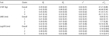
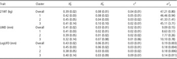
The heritabilities estimated for each trait across all clusters ranged from 0.39 to 0.43 and from 0.32 to 0.45 for each trait within a cluster (Table 4). Cluster 1 had the highest estimates for both UMD and LogUFD, whereas Cluster 2 had the highest estimate for 21WT. Those estimated for Cluster 3 were associated with the highest standard errors, due to the low number of data records. Maternal heritabilities were low and ranged from 0.01 to 0.10. The lowest values were estimated for Cluster 2 whereas the highest values were associated with Cluster 3 for 21WT and UMD, however, these were also associated with high standard errors. Common environmental effects were also low and in most cases were not significantly different from zero.
Univariate direct (h d 2) and maternal (h m 2) heritabilities, common environmental effects (c 2) and phenotypic variances (σ 2 p) between clusters for each trait (s.e. in parenthesis)
21WT=21-week weight; UMD=ultrasound muscle depth; UFD=ultrasound fat depth.
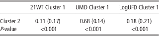
The genetic correlations estimated between Cluster 1 and Cluster 2, for each trait, were all significantly <1 (P<0.001) and are shown in Table 5. The highest correlation was estimated for UMD (0.68) and the lowest for LogUFD (0.18), with the latter not significantly different from zero. Due to the low numbers of connecting sires associated with Cluster 3, as well as the limited data set, the genetic correlations using this cluster are not presented.
Genetic correlations (s.e. in parenthesis) and likelihood ratio P-values estimated between Cluster 1 and Cluster 2 for 21WT, UMD and LogUFD

21WT=21-week weight; UMD=ultrasound muscle depth; UFD=ultrasound fat depth.
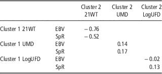
The EBVs of the 53 common sires, used across Cluster 1 and Cluster 2, were further investigated. By using the EBVs for each common sire who had a minimum of 10 offspring in both cluster groups (n=9), the analysis found that a number of the sires re-ranked across the two cluster groups. Spearman’s rank and Pearson’s correlations, are shown in Table 6. Negative correlations were estimated for 21WT whereas low and positive correlations were estimated for UMD. The Spearman’s rank correlation estimated for LogUFD was low and positive, whereas the Pearson correlation estimated was low and negative.
Pearson correlations (EBV) and Spearman’s rank correlations (SpR) between Cluster 1 and Cluster 2

EBV=estimated breeding values; 21WT=21-week weight; UMD=ultrasound muscle depth; UFD=ultrasound fat depth.
Discussion
Clustering techniques, in relation to G×E, have been used in a number of studies using dairy and beef cattle. Previously, individual countries were used as the production environments, such as in the study by Lee and Bertrand (Reference Lee and Bertrand2002). However, by employing this method, such analyses do not take into account the fact that farms in different countries may have similar environments and management systems. The studies carried out by Weigel and Rekaya (Reference Weigel and Rekaya2000) and Espasandin et al. (Reference Espasandin, Urioste, Naya and Alencar2013) are two examples where clusters of farm environments were identified across different countries, thus allowing genetic correlations to be estimated between cluster groups rather than between countries. Similar methods have also been used within countries (Neser et al., Reference Neser, Erasmus and Scholtz2008; Huquet et al., Reference Huquet, Leclerc and Ducrocq2012b).
The variables used to cluster the farms, in the cattle studies mentioned above, often included information such as climatic conditions, performance indicators (such as milk yield or weight at weaning) and herd size. However, in the present study, the extensive nature of sheep farming systems means that many more environmental variables could be involved in influencing the performance of the animals. For this reason, the present analysis investigated whether it was possible to construct clusters of farms with similar environments and management systems using typology techniques. With the exception of the study by Morgan-Davies et al. (Reference Morgan-Davies, Waterhouse and Wilson2012), the present study differed slightly to other typology studies, due to the fact that PCO analysis was used rather than principal component analysis (PCA) (Köbrich et al., Reference Köbrich, Rehman and Khan2003; Gelasakis et al., Reference Gelasakis, Valergakis, Aresenos and Banos2012). Gower (Reference Gower1966), comments that the use of PCA is not suitable when the data set includes qualitative, or discrete data, therefore when considering the mix of quantitative and discrete data used in the current study, PCO was selected.
Early G×E studies using sheep often looked for evidence between breeds, such as those reviewed by Steane (Reference Steane1983), as well as those carried out by Carter et al. (Reference Carter, Carmen, McClaugherty and Haydon1971a, Reference Carter, Carmen, McClaugherty and Haydon1971b and Reference Carter, Carmen and McClaugherty1973). More recently, the effects of different planes of nutrition, as well as different geographical areas, have demonstrated G×E effects (both between and within breeds), in terms of their effects on lamb growth (Osoro et al., Reference Osoro, Olivan, Celaya and Martinez1999; Steinheim et al., Reference Steinheim, Weladji, Skogan, Adnoy, Skjelvag and Holand2004 and Reference Steinheim, Odegard, Adnoy and Klemetsdal2008) and carcass characteristics, (Bishop et al., Reference Bishop, Conington, Waterhouse and Simm1996; Lewis et al., Reference Lewis, Macfarlane, Simm and Emmans2004; Macfarlane et al., Reference Macfarlane, Lewis and Emmans2004). The effects of different nutrition levels on Merino wool production and quality traits have also identified G×E (Dominik et al., Reference Dominik, Crook and Kinghorn1999), whereas environments based on flock milk yield were used by Sanna et al. (Reference Sanna, Carta and Casu2002) to identify G×E for milk yield in Sardinian Sarda sheep. McLaren et al. (Reference McLaren, Lambe, Brotherstone, Conington, Mrode and Bunger2012a and Reference McLaren, Lambe, Brotherstone, Conington, Mrode and Bunger2012b), while assessing the performance of Scottish Blackface ewes and lambs between two contrasting hill farm environments, identified G×E for lamb birth weights and ewe pre-mating weights, but not for lamb 21WT, UMD or UFD.
The increased level of detail gained in the present study was predominantly related to grazing management throughout the season, as well as the provision of supplementary feeding, vitamins and minerals. Studies by both Macfarlane et al. (Reference Macfarlane, Lewis and Emmans2004) and Speijers et al. (Reference Speijers, Carson, Dawson and Gordon2009) demonstrated significant results when breed by feed type interactions were examined. Although the breeds and crossbreeds used in the study by Speijers et al. (Reference Speijers, Carson, Dawson and Gordon2009) were perhaps more associated with hill farming environments, the results demonstrated clear differences between three different diets and between the different breeds used. Macfarlane et al. (Reference Macfarlane, Lewis and Emmans2004) observed significant differences in the growth responses of lambs grazing different sward types, which, along with the results of Speijers et al. (Reference Speijers, Carson, Dawson and Gordon2009), demonstrate that differences in the magnitude of genetic superiority can exist between animals on different grazing types.
In the present study, the farmers were asked to identify where the flock had access to graze throughout the year. They were provided with four different grassland-type options and it was up to the individual farmer in terms of how they classified the different grassland areas of their farm. It may have perhaps been preferable to have more specific grazing options, based on aspects such as sward structure, thus improving the reliability of the data. Nonetheless, the results highlight that differences in grazing-use, throughout the year, are something that should be considered if farm environments are clustered in the future.
Significant weather differences between cluster groups are very likely to have influenced flock management, particularly lambing dates and grazing management, due to effects on length of the grass growth season, quality of grass and animal behaviour. Flocks in Cluster 1, on average, were exposed to the lowest rainfall levels, the highest number of sunshine hours and the highest temperatures throughout the year. In contrast, flocks in Cluster 3 experienced, on average, the highest rainfall, lowest sunshine hours and temperatures throughout the year. Indeed Steinheim et al. (Reference Steinheim, Weladji, Skogan, Adnoy, Skjelvag and Holand2004) found that weather conditions often had a significant effect on the autumn weight (similar to the 21WT in the present study) of lambs in Norway.
The participation in performance and pedigree recording in the UK sheep industry has been aided through the use of AI and embryo transfer, as well as farmers progressively sourcing both male and female stock with EBVs for traits that they wish to improve. Connectedness between flocks (or clusters in this case) is necessary to ensure reliable across-flock/cluster genetic comparisons (Lewis et al., Reference Lewis, Crump, Simm and Thompson1999). Level of connectedness can be quantified through the use of prediction error correlations, also known as connectedness correlations (Lewis et al., Reference Lewis, Crump, Simm and Thompson1999). Kuehn et al. (Reference Kuehn, Lewis and Notter2008) suggests suitable benchmarks for assessing the level of connectedness are 0.05 for ‘good’ and 0.10 for ‘superior’ connectedness. The flocks, and therefore clusters, in the present study were reasonably well linked genetically. The average pairwise levels of connectedness between the clusters, in 2011, were 0.11, 0.05 and 0.07 between Cluster 1 and Cluster 2; Cluster 2 and Cluster 3; and Cluster 1 and Cluster 3 respectively (K. Moore, personal communication). Kuehn et al. (Reference Kuehn, Lewis and Notter2008) also comment that correlations above 0.10 correspond with an ~90% reduction in bias, therefore the correlations calculated between Cluster 1 and Cluster 2 were deemed the most informative and reliable. The lower connectedness correlations associated with Cluster 3 and the other two cluster groups will be related to the low number of common sires used between them (only three flocks in Cluster 3 and low use of technologies such as AI).
The genetic correlations estimated between Cluster 1 and Cluster 2, for 21WT, UMD and LogUFD, were significantly below unity (P<0.001), suggesting the presence of G×E. This was further highlighted by the values obtained from both the Pearson’s and Spearman’s rank correlations, indicating the presence of re-ranking between environments. Robertson (Reference Robertson1959) had previously suggested that only correlations estimated below 0.8 indicated G×E of significance. Whether this value is still relevant is out-with the scope of the present study. The fact that the correlations estimated in the present study were significantly different to unity demonstrates that G×E was evident, therefore potentially impacting on the performance of individual animals as well as the overall flocks involved.
The presence of G×E can reduce genetic gain by lowering the accuracy of selection (Mulder and Bijma, Reference Mulder and Bijma2005). This, in turn, can therefore affect the efficiency of index selection, due to unfavourable variability in terms of both predicted financial and genetic gains, as demonstrated by Dominik and Kinghorn (Reference Dominik and Kinghorn2008). There are three approaches available to breeders in terms of how to deal with G×E, as discussed by McLaren et al. (Reference McLaren, Lambe, Brotherstone, Conington, Mrode and Bunger2012a): (1) ignore G×E, risking poor and somewhat unpredictable performance of the selected animals; (2) avoid G×E by selecting lines with wide adaptability across different environments, for example sires that ranked similarly across the clusters in the present study; (3) exploit G×E by developing locally adapted lines suited to the environments in which they are to be used, such as the sires best suited to specific clusters in the present study.
If the clusters identified in the present study are representative of the UK terminal sire sheep industry overall, the results, particularly between Cluster 1 and Cluster 2, suggest the reliability of genetic evaluations could be improved by taking into account the G×E observed. Providing there are suitable genetic links across clusters, the use of a cluster model would allow an EBV for each animal to be predicted for each environment, thus allowing the identification of animals best suited to specific environments, or animals that will perform consistently across a number of environments, as suggested by Neser et al. (Reference Neser, Erasmus and Scholtz2008). This would potentially reduce any unwanted effects of G×E and allow farmers to select animals best suited to their farm environment.
Alternatively, as discussed by Mulder et al. (Reference Mulder, Veerkamp, Ducro, Van Arendonk and Bijma2006), different breeding strategies may be an option, depending on the level of genetic correlations estimated between the different environments. Mulder et al. (Reference Mulder, Veerkamp, Ducro, Van Arendonk and Bijma2006) observed, while investigating G×E in the dairy industry, that when genetic correlations, estimated between environments, were below 0.61, genetic gain was optimised when there was environment specific breeding programmes progeny testing sires in their specific environment only. If correlations above 0.61 were estimated, a single breeding programme, progeny testing all sires in each environment and applying index selection would be optimal in order to improve performance in all environments simultaneously. Further investigation would be required in order to assess what level of correlation would affect the choice of strategy in relation to sheep breeding as well as the practicalities of progeny testing. For example, financially, from the farmer’s point of view, would the implementation of such a sire progeny testing scheme be cost effective when compared with the potential financial losses that may be incurred through the presence of G×E?
However, if clustering methods were to be further developed, for commercial use, a suitable level of information would be required to ensure the clusters identified were a reliable and true reflection of the different farms systems within the overall industry. It may be an option for future investigation to use only variables readily available for all farms in the United Kingdom, such as those obtained through government census statistics. This would remove the need for farmers to actively respond to an additional survey and increase the number of farms, and therefore data, available for analysis. The additional data would also allow the investigation of breed specific clusters rather than the across breed clusters used in the present study. The clusters would also have to have the ability to incorporate any future changes to the variables involved, as well as accounting for any possible heterogeneity of variances present. The results of the present study also highlight that it is vital all environments are genetically well linked. For example, it may be that if the Texel data were used, the reliability of estimates associated with Cluster 3 would be improved due to the increased number of flocks allocated to this cluster. An alternative option available to breeders would be the potential use of reaction norm models, which rely less on the connectedness between individual farms because the environments are measured on a continuous scale (Huquet et al., Reference Huquet, Leclerc and Ducrocq2012b). Further investigation, using this method, would also be beneficial.
Conclusion
In conclusion, although the analysis presented only provides a ‘snap-shot’ view of the UK terminal sire flock, the subsequent genetic analyses gives some indication of the problems and opportunities that could arise. The increased level of information gathered, particularly in terms of grazing and the use of vitamin and mineral supplements, enabled three distinct clusters to be identified. It remains to be seen, in future studies, if these are representative of the overall terminal sire flock in the United Kingdom, but it does demonstrate the different variables that could be involved in grouping flocks into similar environment and management types. The genetic correlations estimated for all traits investigated, between Cluster 1 and Cluster 2, were all significantly below unity, suggesting the presence of G×E, with those for 21WT and LogUFD particularly low. The evidence of Charollais sires re-ranking between Cluster 1 and Cluster 2 suggest that the performance of their offspring was being controlled by different genes in different environments. Providing a suitable strategy can be identified, there is potential for improving the efficiency of future sheep breeding programmes, by taking into account the G×E observed. This would enable farmers to identify and select animals with an increased knowledge as to how they will perform in their specific farm environment thus reducing any unexpected differences in performance. The study has also highlighted a number of areas worthy of future investigation in order to strengthen the implications and conclusions reached.
Acknowledgements
The author wishes to acknowledge EBLEX, HCC & QMS for funding this research. Many thanks also to the farmers who responded to the questionnaire, Sam Boon at Signet Breeding Services and Kirsty Moore at EGENES for their help with providing the data.