2.1. Governing Equation in the Weakly Nonlinear Approximation

Let us consider our system as consisting of a mobile cold electronic fluid and a neutralizing fixed ionic background.

In the co-moving regime we will be investigating, all field amplitudes, radiation, and wakes, are assumed to propagate along the x axis of our coordinate system with a given nonlinear group velocity v _g whose magnitude must be found.

Starting with the laser field, we take it to be described by the associated vector potential A, which is represented in the form

(1)$${\bf A} = \hat{\bf z}a\lpar {\bf x}_ \bot\comma \; x - v_g \, t\rpar e^{i\lpar k_0 x - {\rm \omega} _0 t\rpar } + c.c.$$

The variable a is the slowly varying real amplitude of the field, with k ₀ and ω₀, respectively, as the wave vector and frequency of the high-frequency carrier. We note that in accordance with all the previous comments on the field structure, in addition to the co-moving coordinate ξ ≡ x − v _gt, we allow for the inclusion of the transverse structure represented by the transverse coordinate x_⊥ in the argument of the scalar amplitude a. The interdependence of the carrier's frequency and wave vector with the group velocity v _g, shall be elucidated as soon as one solves the wave equation for the vector potential A.

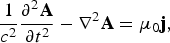
In the Coulomb gauge, the laser wave equation reads

(2)$$\displaystyle{1 \over {c^2 }} \displaystyle{{\partial ^2 {\bf A}} \over {\partial t^2 }} - \nabla ^2 {\bf A} = {\rm \mu} _0 {\bf j}\comma \;$$

where the high-frequency current j can be written in terms of the density n, the electron charge and mass q, m, respectively, the relativistic factor γ, and the vector potential as j =− (q ²/m) n A/γ Gibbon (Reference Gibbon2007). Then, from Eq. (2) one can write the governing equation for the weakly relativistic amplitude a in the form

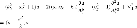(3)$$\eqalign{&- \lpar k_0^2 - {\rm \omega} _0^2 + 1\rpar a - 2i\lpar {\rm \omega} _0 v_g - k_0 \rpar \displaystyle{{\partial a} \over {\partial {\rm \xi} }} - \lpar v_g^2 - 1\rpar \displaystyle{{\partial ^2 a} \over {\partial {\rm \xi} ^2 }}+\nabla_{\bot}^2 a \cr &= \lpar n - \displaystyle{a^2 \over 2}\rpar a.}$$

We point out that in Eq. (3) we have migrated to dimensionless quantities defined in the form ω_px/c → x, ω_px_⊥/c → x_⊥, ω_pt → t, qa/mc ² → a, v _g/c → v _g, and (n − n ₀)/n ₀ → n. The parameter n ₀ is the equilibrium density, ω_p = n ₀q ²/ε₀m denotes the plasma frequency, and μ₀ and ε₀ are the magnetic and electric vacuum permeabilities. We note that the frequency and wave vector of the carrier are normalized likewise, and that the weakly nonlinear (or weakly relativistic) field magnitudes satisfy the condition |qa/mc ² | ≪ 1. On the right-hand side of Eq. (3) the nonlinear features of the theory can be devised: the ponderomotive nonlinearity represented by the coupling involving density and vector potential, and the cubic relativistic nonlinearity, which has its origins in the weakly relativistic expansion of the relativistic factor γ.

One can advance a step further with the analysis as one realizes that a is real. Then, on separating Eq. (3) into its real and imaginary parts the following expressions are obtained,

(4)$$- {\rm \delta} a + {\rm \kappa} \displaystyle{{\partial ^2 a} \over {\partial {\rm \xi} ^2 }} + \nabla_\bot ^2 a=\left( n - \displaystyle{{a^2 } \over 2}\right) a\comma \;$$

(5)$$v_g = \displaystyle{{k_0 } \over {{\rm \omega} _0 }}.$$

The detuning parameter, introduced as δ ≡ k ₀² − ω₀² + 1, is thus seen to be part of a nonlinear equation. As we shall elaborate better in the coming sections, this indicates that wave frequency and wave vector are related through a nonlinear dispersion relation, and that v _g is thus a nonlinear group velocity. On the other hand, the parameter κ ≡ 1 − v _g², here defined in a slightly different way than in a previous paper (Bonatto et al., Reference Bonatto, Pakter and Rizzato2011) to avoid negative values for it, is directly related to the group velocity of the radiation. It becomes small in underdense conditions where the plasma density is small and v _g→1. In what follows, we consider ω₀ > 0, k ₀ > 0, and v _g > 0.

As for the low-frequency density fluctuations, one starts from the ponderomotive-driven low-frequency momentum equation for the electrons and uses the Poisson and continuity equations to obtain the following governing equation under the same set of normalizations previously employed:

(6)$$v_g^2 \displaystyle{{\partial ^2 n} \over {\partial {\rm \xi} ^2 }} + n = \displaystyle{1 \over 2}\displaystyle{{\partial a^2 } \over {\partial {\rm \xi} ^2 }}+\displaystyle{1 \over 2}\nabla_\bot ^2 a^2.$$

For convenience, we split the derivatives of the ponderomotive term on the right-hand side into longitudinal and perpendicular components.

We now proceed to reduce Eqs. (4) and (6) into a simpler and more amenable form for numerical and analytical investigations, avoiding underdense approximations where the velocity of the laser pulse is approximated by the speed of light.

Eq. (6) suggests a convenient combination of fields a ² and n into a new quantity φ ≡ v _g²n − a ²/2, which we call the space-charge potential. Accordingly, regrouping of terms in Eqs. (3) and (5) so as to replace v _g²n − a ²/2 with φ, yields the following coupled equations for the laser field and for the space-charge potential, respectively:

(7)$${\rm \kappa} \displaystyle{{\partial ^2 a} \over {\partial {\rm \xi} ^2 }} = {\rm \delta} a + \displaystyle{1 \over {v_g^2 }}{\rm \varphi} \, a + \displaystyle{{\rm \kappa} \over {2v_g^2 }}a^3 - \nabla_\bot ^2 a\comma \;$$

(8)$$\displaystyle{{\partial ^2 {\rm \varphi} } \over {\partial {\rm \xi} ^2 }} + \displaystyle{1 \over {v_g^2 }}{\rm \varphi} = - \displaystyle{1 \over {2v_g^2 }}a^2 + \displaystyle{1 \over 2}\nabla _ \bot ^2 a^2.$$

The pair of Eqs. (7) and (8) casts itself into the convenient format we were looking for. If the transverse structure is neglected, the set becomes similar to models analyzed in the past (Mofiz & de Angelis, Reference Mofiz and de Angelis1985). Under this planar condition, one can think of Eqs. (7) and (8) as describing the coupled nonlinear dynamics of fields a and φ as a function of the co-moving coordinate ξ, which plays the role of time. With the transverse structure included, the set of Eqs. (7) and (8) describes the weakly nonlinear full spatio-temporal interaction of laser and space-charge field. Coordinate ξ can still be seen as time, and space is associated with the transverse structure itself. We also point out that, in the present regime where fields depend on time through the co-moving coordinates, the presence of the nonparaxial derivative with respect to ξ in Eq. (7) is the chiefly responsible for advancing the laser field in time.

2.2. Beam geometry, Boundary Conditions and the Linearized Model

We first of all observe that solutions to the nonlinear Eqs. (7) and (8) depend on the geometry of the beam. In the present investigation, we adopt a slab geometry where the beam is uniform along one transverse cartesian axis, say z, and is localized along the other one, which we call x _⊥. This option avoids issues related to the inherent singularities at the axis of a cylindrical beam, but is nevertheless qualitatively similar to the cylindrical case if one looks at the half space x _⊥ ≥ 0, provided that the beam is symmetrical with respect to x _⊥ = 0.

In summary, we require that all fields are even functions of the transverse coordinate x _⊥, vanishing as |x _⊥| → ∞.

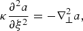
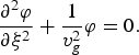
With the geometry and boundary conditions thus defined, we can make progress toward the solution as we note that the linearized version of set (7) and (8)

(9)$${\rm \kappa} \displaystyle{{\partial ^2 a} \over {\partial {\rm \xi} ^2 }} = - \nabla _ \bot ^2 a\comma \;$$

(10)$$\displaystyle{{\partial ^2 {\rm \varphi} } \over {\partial {\rm \xi} ^2 }} + \displaystyle{1 \over {v_g^2 }}{\rm \varphi} = 0.$$

has an analytical solution. φ indeed oscillates with linear frequency 1/v _g while a can be resolved as

(11)$$a\lpar x_\bot\comma \; {\rm \xi} \rpar = a_0 e^{\left[{\left({{\textstyle{{\rm \lambda} \over {\rm \kappa} }}} \right){\rm \xi} ^2 - {\rm \lambda} x_ \bot ^2 } \right]} \cos\left({\displaystyle{{2 \, {\rm \lambda} \, x_\bot {\rm \xi} } \over {\sqrt {\rm \kappa} }}} \right)\comma \;$$

if one Fourier analyzes Eq. (9) along its transverse coordinate x _⊥ and considers a general, initially static condition expressing the idea of localization or focusing: a(x _⊥, ξ = 0) = a ₀e ^{−λx _⊥2}, from where one can clearly see that the dimensional version of λ has the same dimension of 1/x _⊥². Here we take δ = 0 for simplicity, but this condition suffices for future purposes.

Eq. (9) is an elliptic equation similar to the Laplace equation, and its solution, Eq. (11), exhibits the expected exponentially growing behavior along ξ with the characteristic scale given by ${\rm \xi}^ {\ast} \equiv \sqrt {{\rm \kappa} /{\rm \lambda} } $. As nonlinear terms are added to the model, the exponential growth is likely to be saturated at some point. Our interest in what follows is to understand the competing roles of nonlinearity and the intrinsic exponential growth associated with the linear approximation. For further purposes, we point out that the exponential growth along the beam frame coordinate ξ can be seen as a spatio-temporal growth in the laboratory coordinates.

To conclude this section, we simply emphasize that the set (7) and (8) represents our basic model and provides the tools to analyze a myriad of problems, like soliton formation, wakefield excitation, and laser focusing.

Among these various problems, the present paper discusses initially focused beams and their subsequent dynamics.

3.1. Equilibrium Solutions

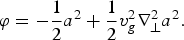
The equilibrium focused beam is the one where the beam transversal profile does not depend on the longitudinal “time” variable ξ. If this is the case, one can promptly write down from Eq. (8) the following expression for the space-charge potential ϕ in terms of the laser field:

(12)$${\rm \varphi} = - \displaystyle{1 \over 2}a^2 + \displaystyle{1 \over 2}v_g^2 \nabla_ \bot ^2 a^2.$$

Eq. (12) also represents the space-charge field under adiabatic conditions, where the the plasma wave frequency is much larger than the typical modulational frequency of the driving laser field.

The potential φ thus obtained from Eq. (12) can be inserted into Eq. (7) to generate the following differential equation for the equilibrium laser beam:

(13)$$\nabla_ \bot ^2 a = {\rm \delta} a - \displaystyle{1 \over 2} a^3 + \displaystyle{1 \over 2}a \nabla_\bot ^2 a^2.$$

If from Eq. (13) we wish to create a radiation beam symmetrical with respect to the transverse coordinate, suffice is to work in the half-space x _⊥ ≥ 0, demanding that da/dx _⊥ |_{x ⊥=0} = 0 and that a(x _⊥→∞)→0. Denoting a _eq as the equilibrium solution, the problem thus formulated admits an analytical solution of the form

(14)$$a_{eq}^{analytical} = \sqrt {4{\rm \delta} } \, {\rm sech}\left( {\sqrt {\rm \delta}} x_\bot\right) \comma \;$$

when the nonlinear term containing the Laplacian is ignored. We see from Eq. (14), for instance, how both amplitude and transverse length at equilibrium scale with the detuning δ. In particular, since δ defines the field amplitude, the frequency and wave vector of the carrier are related by a nonlinear dispersion relation, as alluded to earlier. The detuning δ (whose dimensional version has the same dimension of 1/x _⊥²), can also be seen as playing the role of the length scale λ at equilibrium.

The analytical solution is far from being inaccurate, because the discarded term leading to it is small. However, since we shall be dealing with unstable equations in the dynamics, it is recommended that all terms be kept. With all terms included, we take the following numerical procedure to construct solutions. Imposing the zero derivative condition at x _⊥ = 0, we search for an initial amplitude a ₀ ≡ a(x _⊥ = 0) that causes a to asymptotically approach zero as x _⊥ grows. The numerically found solutions will tend to and stay close to zero for a long stretch along the x _⊥-axis, but will eventually depart from this smallness condition. Numerical accuracy can be improved if we work out the digits of a ₀ in such a way that the solutions asymptotically stay close to a = 0 for increasingly longer stretches.

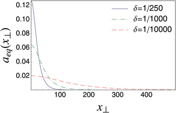
In Figure 1, we display a series of curves of a _eq (x _⊥) versus x _⊥ for different values of the detuning parameter δ, the only control parameter present in the equilibrium equation (14). The detuning δ must be positive to generate a nontrivial solution, but small to guarantee smallness of field a _eq. We nevertheless see from Figure 1 that even for small detunings, the field profile largely varies with their exact values. As one moves from smaller to larger values of δ, the profiles become sharper, with larger amplitudes and narrower widths.

Fig. 1.

(Color online) Plots of a _eq(x _⊥) versus x _⊥ for various values of the detuning factor δ.

Once the equilibrium solutions have been found, we are in position to investigate the system behavior when initial conditions are launched in the neighborhood of these equilibria regimes. In other words, how does a mismatched radiation beam evolve as a function of beam-frame coordinate ξ? We address this issue as our next section.

3.2. Simulations of the Spatio-temporal Dynamics

3.2.1. Initial Remarks and the Linear Dynamics

Before entering in the study of the complete system, one should perhaps conduct a test comparing the analytical solution provided by Eq. (11) with simulations of the linear version of Eqs. (7) and (8). This first test helps to tune up simulation parameters, so that the corresponding results become as accurate as possible. We point out that this kind of test is important, given the fact that the elliptic nature of our system demands high numerical precision.

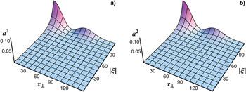
Simulations make use of a uniform mesh along x _⊥ to evaluate the corresponding Laplacian with finite differences. The fields at each node are advanced in ξ with an adaptive Runge-Kutta time integrator. We use N = 256 to N = 1024 nodes, along with a tolerance factor of 10⁻¹⁰, and the differences are minimal. The simulation shown in Figure 2a was done with N = 512 and indeed displays nice agreement with the analytical results of corresponding panel (b). We also use λ = 0.0001 and a slightly underdense case κ = 0.5. Note that in the regime we are investigating, the forward moving wave front is located at ξ = 0 and we look at fields behind it with ξ < 0. This is why we represent the “time” in terms of its absolute value |ξ|. Note that although we work in a underdense regime, the typical underdense approximation v _g → c is totally avoided, as promised in our introductory remarks.

Fig. 2.

(Color online) Comparing the space-time simulation code as applied to Eq. (10), panel (a), with the corresponding analytical result provided by Eq. (9), panel (b). We take λ = 0.0001 and κ = 0.5.

3.2.2. Matched Beams

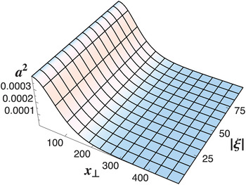
Attention is next drawn toward the nonlinear spatio-temporal case. In our first look into the problem, we use the equilibrium solution yielded by the solution of Eq. (12) as the initial condition for our simulations based on Eqs. (7) and (8). The corresponding results are shown in Figure 3. One sees that the profile indeed remains unaltered for periods of time longer than the time scale ξ* defined in the context of Eq. (11), which in our dimensionless form reads approximately ξ*~70 for the simulation parameters δ = 0.0001, v _g² = 0.5 used here to illustrate the study. The growth scale is even shorter if one adds the destabilizing effects of the positive detuning absent in Eq. (11) but present in Eqs. (7) and (13)—the scale drops to ξ*~50. This fact suggests that the code, with all its nonlinear terms, remains robust against the known instabilities of the elliptic problem. As seen from our normalizations and from the approximate expression for equilibrium furnished by Eq. (13), the choice δ = 0.0001 defines transverse length scales containing around 100 plasma wavelengths. This choice is quite compatible with experimental set-ups (Jha et al., Reference Jha, Malvyia and Upadhyay2010) and shall be used throughout the paper.

Fig. 3.

(Color online) Testing the numerical code in equilibrium regimes. Here we take δ = 0.0001 and κ = 0.5.

3.2.3. Mismatched Beams

We finally address issues concerning the behavior of initially mismatched radiation beams. As we start off from nonequilibrium initial conditions, the interest is to see whether or not beams remain nearly focused if the initial mismatches are relatively small. In other words, a stability analysis shall be performed here.

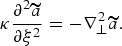
We had observed earlier that the linear version of our basic set is unstable in the sense that Eq. (9) predicts exponential growth for a(x _⊥, ξ) as ξ advances. The reflex of this feature on the stability of equilibrium solution comes out as follows. If one takes the equilibrium solution a _eq for the laser field and perturb it with a small fluctuation ${\widetilde a}$ displaying sufficiently strong dependence on the transverse coordinate x _⊥, the equation governing ${\widetilde a}$ takes approximately the linear form already seen in Eq. (9):

(15)$${\rm \kappa} \displaystyle{{\partial ^2 \widetilde a} \over {\partial {\rm \xi} ^2 }} = - \nabla_\bot ^2 \widetilde a.$$

Small perturbations thus grow with ξ, the signature of an unstable process. Even fields with more smoothly dependence on x _⊥ have spectral components at high values of the respective wave vector, so we expect instability in general, and not only when the dominant length scale of the perturbation is short.

The growing solution is eventually saturated by the nonlinear terms of the full set of equations, and we now attempt to offer a view of the whole process.

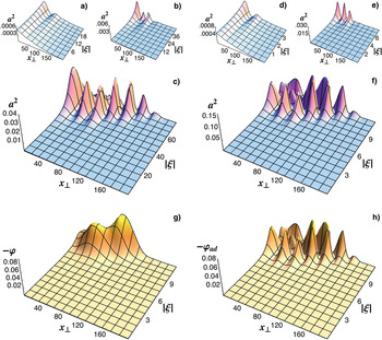
In Figure 4, we display several panels analyzing the time evolution of fields a and φ at various time scales along the ξ axis. The initially mismatched beam is written in the form

(16)$$a\lpar x_\bot\comma \; {\rm \xi} = 0\rpar = a_{eq} \lpar x_ \bot\comma \; {\rm \xi} = 0\rpar + {\rm \epsilon} a_{eq} \lpar {\rm \chi} x_ \bot\comma \; {\rm \xi} = 0\rpar \comma \;$$

with φ(x _⊥, ξ = 0) = φ_eq. Fields a _eq and φ_eq are the equilibrium fields obtained in the previous subsection, ε≪1 is a small parameter measuring the strength of the perturbing term, and χ is a scale factor indicating the dominant length scale of the perturbing term. Larger values χ > 1 represent shorter transversal scales as compared to that of the equilibrium profile, and vice-versa. Let us consider δ = 0.0001, χ = 10, and ε = 0.2 in all cases of Figure 4, with κ = 0.5 for the first three panels, (a) to (c), and a more deeply underdense regime with κ = 0.01 for the last five panels (d) to (h). At the short times of panel (a) one can identify the exponential growing pattern typical of the linear regime for the laser field. Panel (b) still displays growing solutions and panel (c) finally reveals the saturation process following strong focusing near x _⊥ = 0. As the initially growing mismatched solution reaches saturation, the beam breaks up into a seemingly irregular space-time pattern of beamlets and any coherence is lost. One sees that within the time scale displayed in Figure 4, the largest field amplitudes a lie quite within the weakly nonlinear regimes of laser wakefield accelerator settings (Mora & Antonsen, Reference Mora and Antonsen1997). For longer times the irregular pattern progresses on, accompanied by spikes whose amplitudes lie beyond our weakly nonlinear assumptions.

Fig. 4.

(Color online) Full space-time history for the mismatched radiation beams at various time scales along the ξ axis, both in higher and lower density conditions. Panels (a) to (c) refers to laser amplitude in the higher density case κ = 0.5, and panels (d) to (f) to the laser amplitude in a low density underdense case κ = 0.01. In panels (g) and (h) the space-charge potential φ is shown for κ = 0.01; the actual potential in panel (g) follows the adiabatic dynamics of panel (h) only up to point where the beam breaks up. In all cases δ = 0.0001 and χ = 10.

Panels (d) to (f) represent a low-density case with κ = 0.01, which is more akin to underdense settings of wakefield accelerators, for instance. The laser patterns are similar to the previous case, but now one can notice that the development of the instability is much faster than the one seen in the κ = 0.5 case. Indeed, the scalings suggested in Eq. (6) indicate that, keeping the same initial profile (same λ), instability for the smaller value of κ should be approximately seven-fold faster than the one for the larger value.

In panels (g) and (h), we respectively compare the actual space-charge potential φ with its adiabatic approximation, let us call it φ_ad, earlier discussed in the context of Eq. (12). Given the initial smoothness of the radiation beam it is seen that the actual space-charge field initially follows an adiabatic dynamics, but only up to the point where the beam breaks up into the series of beamlets. Afterward the time scales for the wakes become comparable to the plasma wave scales. We use κ = 0.01 in panels (g) and (h).

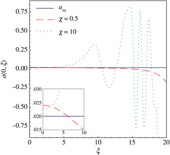
As we mentioned, the above study for χ = 10 represents those cases where initial mismatches have shorter length scales if compared to the length scale of the equilibrium profile. We commented that perturbations with longer length scales also grow, but still, it may be interesting to pinpoint the differences between the latter and former cases. The subject is examined in Figure 5, where we plot of curves of a(x _⊥ = 0, ξ) versus ξ for mismatched beams of the form given by Eq. (16). The cases χ = 10 and χ = 0.5 are compared for κ = 0.01, with all the remaining parameters as previously. Short length scales display the more conventional behavior of unstable cases: as the perturbation is created, the corresponding solution simply grows away from the equilibrium solution. However, when the long length scale represented by χ = 0.5 is considered, the mismatched solution is initially attracted by the equilibrium and only then moves away as seen in the inset. The remarkable fact is that mismatches with long length scales behave like stable perturbations until one reaches the time scale of exponential growth, where the initial solution depart from the vicinity of equilibrium.

Fig. 5.

(Color online) Dependence of the dynamical behavior on the mismatch scale χ. Longer scales tend to be display slower growths.