





1 Introduction
Trisections of oriented compact 4-manifolds were introduced by Gay and Kirby in [Reference Gay and Kirby7], who established existence and uniqueness in the closed setting. In the relative setting—that is, for oriented compact 4-manifolds with boundary—a relative trisection induces an open book decomposition on the boundary. Gay and Kirby show existence of relative trisections inducing any given open book on the boundary, and uniqueness (up to stabilization) given a fixed open book on the boundary. This uniqueness result was improved in Castro’s PhD thesis [Reference A. Castro2] by the introduction of relative stabilizations. Castro–Islambouli–Miller–Tomova [Reference Castro, Islambouli, Miller and Tomova6] obtained a full uniqueness result by introducing relative double twists.
In this article, we introduce pseudo-trisections, an alternative framework for studying 4-manifolds with boundary. Rather than inducing open book decompositions on the boundary, they induce 3-manifold trisections in the sense of Koenig [Reference Koenig12]. Since Heegaard splittings induce 3-manifold trisections in a canonical way, pseudo-trisections can be thought of as an interpolation between Heegaard splittings of boundary 3-manifolds and classical trisections of 4-manifolds. We prove an analogous existence result to the aforementioned result of Gay–Kirby.
Theorem 1.1 Let X be a compact oriented smooth 4-manifold with non-empty connected boundary Y. Let
$\tau $
 be a trisection of Y. Then there is a pseudo-trisection of X which restricts to
$\tau $
 on the boundary.
On the other hand, we define three types of stabilization (internal, boundary, and Heegaard) for pseudo-trisections, two of which extend notions of stabilization defined for 3-manifold trisections. We show uniqueness of pseudo-trisections up to these moves.
Theorem 1.2 Let X be a compact oriented smooth 4-manifold with non-empty connected boundary. Any two pseudo-trisections of X are equivalent up to internal, boundary, and Heegaard stabilization.
The main feature of pseudo-trisections is that they are general enough to exist with lower complexity than relative trisections. Complexity is an analog of trisection genus and is defined in Section 3. Pseudo-trisections of complexity at most 1 are classified and observed to be richer than relative trisections of equal complexity. Example 3.30 shows that
$c(\natural ^\ell (S^2\times D^2)) \leq \ell $
 among pseudo-trisections, whereas we expect that
$c(\natural ^\ell (S^2\times D^2)) \geq 3\ell $
 among relative trisections. (The latter would be true if relative trisection genus were additive under connected sum.)
We also introduce pseudo-trisection diagrams as a method for representing pseudo-trisections, analogously to trisection diagrams [Reference Gay and Kirby7] and relative trisection diagrams [Reference Gay, Pinzón-Caicedo and Castro24]. In each of these settings, diagrams are shown to be in one-to-one correspondence with (relative) trisections when modding out by appropriate moves. We obtain an analogous result:
Theorem 1.3 The realization map

induces a bijection

Combined with the seeming lower complexity of pseudo-trisections, this results in a diagrammatic theory for 4-manifolds with boundary with lower complexity than relative trisection diagrams. Along the way, we introduce triple Heegaard diagrams to represent trisections of closed 3-manifolds, and the calculus thereof. This diagrammatic calculus incorporates moves inspired by Heegaard theory and plumbing of open books. A pseudo-trisection diagram of a pseudo-trisected 4-manifold has the convenient property of restricting to a triple Heegaard diagram of the induced trisection on the boundary 3-manifold. Consequently, pseudo-trisection diagrams can also be thought of as combining the theory of trisection diagrams and (roughly) Heegaard diagrams.
In the final section of the article, we extend our diagrammatic calculus from 4-manifolds with boundary to pairs
$(X, \mathcal K)$
 where
$\mathcal K$
 is a surface embedded in X in pseudo-bridge position. This generalizes the theory of bridge trisections introduced by Meier–Zupan [Reference Meier and Zupan18] in the closed setting, and by Meier [Reference Meier17] in the relative setting. Pseudo-bridge trisections are defined to be compatible with pseudo-trisections, in much the same way that relative bridge trisections are compatible with relative trisections. Consequently we can define pseudo-shadow diagrams, which consist of an underlying pseudo-trisection diagram to encode the ambient 4-manifold, and additional arcs to encode the embedded surface.
We finish by exploring several examples of pseudo-shadow diagrams, such as a Möbius strip in
$\mathbb {CP}^2 - B^4$
 , and a slice disk of a trefoil knot in
$\mathbb {CP}^2 - B^4$
 . Through these examples we demonstrate how to compute some invariants from pseudo-shadow diagrams, namely Euler characteristic, orientability, and homology class.
1.1 Conventions
Hereafter Y refers to connected closed smooth 3-manifolds, and X to compact smooth oriented 4-manifolds with one boundary component. The boundary of X is denoted by Y. The indices i and j are taken to be in
$\mathbb {Z}/3\mathbb {Z}$
 . Bolded symbols such as
$\boldsymbol {k}$
 and
$\boldsymbol {y}$
 represent triples of three non-negative integers
$k_1, k_2, k_3$
 , or
$y_1, y_2, y_3$
 . We write
$|\boldsymbol {k}|$
 to mean the 1-norm, which in this case is just the sum of the
$k_i$
 . We also write
$\boldsymbol \delta $
 and
$\boldsymbol \alpha $
 to represent certain collections of loops. The loops themselves are unbolded, for example
$\delta _1$
 or
$\alpha $
 .
We say
$N \subset M$
 is neatly embedded if
$\partial N \subset \partial M$
 , and N is transverse to
$\partial M$
 . Unless otherwise stated, any arcs in surfaces with boundary or 3-manifolds with boundary are assumed to be neatly embedded. We write
$\mathcal K$
 to denote a connected compact surface with boundary neatly embedded in X. The boundary of
$\mathcal K$
 is a link L in Y.
1.2 Organization of the article
In Section 2, we review 3-manifold trisections and introduce triple Heegaard diagrams. In Section 3, we introduce pseudo-trisections, three notions of stabilization, and prove Theorem 1.2. Further, pseudo-trisection are compared with relative trisections. In Section 4, we introduce pseudo-trisection diagrams, and prove Theorems 1.1 and 1.3. In Section 5, we introduce pseudo-bridge trisections and pseudo-shadow diagrams, and study several examples.
2 Trisections of 3-manifolds
In this section, we summarize some definitions concerning trisections of 3-manifolds, introduced by Dale Koenig [Reference Koenig12]. In particular, we describe stabilizations and Koenig’s result that (almost all) 3-manifold trisections are stably equivalent in this more general sense. Next, we introduce Heegaard stabilizations, inspired by stabilizations of Heegaard splittings. We show that any two trisections for any 3-manifold are equivalent up to stabilization and Heegaard stabilization. Next, we introduce triple Heegaard diagrams, an analog of Heegaard diagrams for trisections of 3-manifolds. Finally we briefly discuss complexity of 3-manifold trisections.
2.1 3-manifold trisections and stabilization
In this subsection, we review the theory of 3-manifold trisections introduced in [Reference Koenig12].
Definition 2.1 [Reference Koenig12]
A
$(\boldsymbol {y}, b)$
 -trisection of a 3-manifold Y is a decomposition
$Y = Y_1 \cup Y_2 \cup Y_3$
 such that
-
• each $Y_i$
 is a handlebody of genus
$y_i$
,
-
• each $\Sigma _{i} = Y_{i-1} \cap Y_i$
is a compact connected surface with some genus
$p_i$
and boundary B, and -
• $B = Y_1 \cap Y_2 \cap Y_3$
is a b-component link.





The link
$B \subset Y$
 is the binding of the trisection. See Figure 1 for a schematic for how the pieces fit together.
The components of a trisection of a 3-manifold Y.

Proposition 2.2 3-manifold trisections satisfy the following properties:
-
(1) Each $y_i$
is given by
$p_i + p_{i+1} + b - 1$
. In particular,
$y_i$
is bounded below by
$b-1$
. -
(2) The genera $p_i$
of the surfaces
$\Sigma _i$
are given by
$\frac {1}{2}(y_{i-1} + y_i - y_{i+1} - b + 1)$
.





Proof The first fact follows from the fact that
$Y_i$
 is a handlebody with boundary
$\Sigma _i \cup \Sigma _{i+1}$
 , where the surfaces are identified along their boundaries. The second fact is obtained by solving the simultaneous equations in the first fact.
Example 2.3 The trivial trisection is a decomposition of
$S^3$
 into three 3-balls, with any two balls meeting along a common disk. The triple intersection of these balls is an unknot.
Example 2.4 Every 3-manifold admits a trisection: one construction is to start with a Heegaard splitting
$Y = H_1 \cup H_2$
 . Then consider a contractible loop
$\gamma $
 on
$\Sigma = \partial H_1$
 . This bounds a disk D in
$\Sigma $
 , and a neatly embedded parallel disk
$D'$
 in
$H_1$
 (by isotoping D). The surface
$D\cup D'$
 bounds a ball B in
$H_1$
 . Now

is a trisection of Y, with
$B = \gamma $
 .
Another recipe to construct trisections is to start with an open book decomposition. Details for this example (and further examples) are provided in [Reference Koenig12].
Example 2.5 There is a (non-unique) connected sum of trisected 3-manifolds. Specifically one can delete a standard neighborhood of a point in the binding of two trisections. Now each 3-manifold has spherical boundary, and the spheres have induced decompositions into three wedges. An (oriented) connected sum along these spheres respecting the decomposition into wedges produces a trisection of the connected sum of the 3-manifolds.
Definition 2.6 Given a trisection
$(Y_1, Y_2, Y_3)$
 of a 3-manifold Y, a stabilization is a new trisection
$(Y_1', Y_2', Y_3')$
 constructed as follows:
-
(1) Choose a neatly embedded non-separating arc $\alpha $
in
$\Sigma _i$
for some
$i \in \{1,2,3\}$
. (Such an arc exists provided
$\Sigma _i$
is not a disk.) -
(2) Let $N(\alpha )$
be a tubular neighborhood of
$\alpha $
in Y, and define-
• $Y_{i+1}' = Y_{i+1} \cup \overline {N(\alpha )}$
, -
• $Y_{i}' = Y_{i} - N(\alpha )$
, -
• $Y_{i-1}' = Y_{i-1} - N(\alpha )$
.
-





See Figure 2 for a schematic of stabilization, given a non-separating arc
$\alpha $
 in
$\Sigma _1$
 .
A stabilization of a trisection of a 3-manifold.
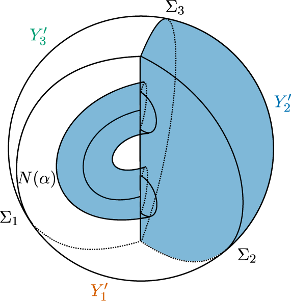
Notice that stabilization increases
$y_{i+1}$
 by 1 while leaving
$y_i$
 and
$y_{i-1}$
 unchanged. On the other hand, b increases by 1 if both endpoints of
$\alpha $
 are in the same component of B, and decreases by 1 if the endpoints are in different components. See [Reference Koenig12] for examples of stabilizations.
Remark 2.7 Provided Y is not
$S^3$
 , any trisection of Y can be stabilized, since at least one
$\Sigma _i$
 must not be a disk. In Section 2.2, we introduce a second notion of stabilization to deal with the
$S^3$
 case.
We say that two trisections
$\mathcal {T}$
 and
$\mathcal {T}'$
 of Y are isotopic if there is a diffeomorphism from Y to itself, isotopic to the identity, sending the ith sector of
$\mathcal {T}$
 to the ith sector of
$\mathcal {T}'$
 . Further, we say a trisection is a stabilization of another if it can be obtained by a finite sequence of stabilizations up to isotopy. Two trisections are said to be equivalent up to stabilization or stably equivalent if there is a third trisection which is a stabilization of each of the other two.
Theorem 2.8 (Koenig [Reference Koenig12])
Let
$\mathcal {T}, \mathcal {T}'$
 be two trisections of a closed orientable 3-manifold Y. If Y is the 3-sphere, assume neither trisections are the trivial trisection. Then
$\mathcal T$
 and
$\mathcal T'$
 are equivalent up to stabilization.
2.2 Heegaard stabilization
In this subsection, we introduce Heegaard stabilization.
Definition 2.9 Given a trisection
$(Y_1, Y_2, Y_3)$
 of a 3-manifold Y, a Heegaard stabilization is a new trisection
$(Y_1', Y_2', Y_3')$
 constructed as follows:
-
(1) Choose a neatly embedded boundary parallel arc $\alpha $
in
$Y_i$
, with both endpoints on
$\Sigma _i$
. -
(2) Let $N(\alpha )$
be a tubular neighborhood of
$\alpha $
in Y, and define-
• $Y_{i+1}' = Y_{i+1}$
, -
• $Y_{i}' = Y_{i} - N(\alpha )$
, -
• $Y_{i-1}' = Y_{i-1} \cup \overline {N(\alpha )}$
.
-




See Figure 3 for a schematic of Heegaard stabilization, given a non-separating arc
$\alpha $
 in
$Y_1$
 with endpoints on
$\Sigma _1$
 . Requiring
$\alpha $
 to be boundary parallel ensures that each new sector is a 3-dimensional 1-handlebody.
A Heegaard stabilization of a trisection of a 3-manifold.

Figure 3: Long description
A spherical diagram is divided into three sectors by three surfaces meeting at a central vertical axis. The surfaces are labeled Sigma sub 1 on the left, Sigma sub 2 on the bottom right, and Sigma sub 3 at the top. The regions between these surfaces are labeled with prime notation: Y sub 3 prime in teal on the upper left, Y sub 2 prime in blue on the right, and Y sub 1 prime in orange at the bottom. A stabilization feature, labeled N(alpha), is depicted as a curved, tubular handle or loop that originates from the central axis and extends into the teal-shaded region of Sigma sub 1. This loop is drawn with solid lines for visible edges and dotted lines for hidden or interior paths, illustrating a topological modification to the trisection structure.
Heegaard stabilization increases
$y_i$
 and
$y_{i-1}$
 by 1 while leaving
$y_{i+1}$
 and b unchanged.
Proposition 2.10 Any two trisections of a closed orientable 3-manifold are equivalent up to stabilization and at least one Heegaard stabilization.
Proof If a trisection is trivial, Heegaard stabilizing once produces a non-trivial trisection. This means that applying at most one Heegaard stabilization, the trisections can be assumed to be non-trivial. The trisections are now equivalent up to stabilization, by Theorem 2.8.
2.3 Triple Heegaard diagrams
In this subsection, we introduce triple Heegaard diagrams, which are diagrams for 3-manifold trisections adapted from Heegaard diagrams. Given a
$(\boldsymbol {y}, b)$
 -trisection of a 3-manifold, a triple Heegaard diagram will consist of
$|\boldsymbol y|$
 closed curves on surfaces, with each set of
$y_i$
 curves determining a handlebody. This is analagous to Heegaard diagrams requiring
$g+g$
 closed curves, with each set of g curves determining a handlebody.
Definition 2.11 A cut system of curves on a closed surface
$\Sigma $
 of genus g is a collection of g disjoint simple closed curves that cut
$\Sigma $
 into a sphere with
$2g$
 boundary components.
Definition 2.12 A
$(\boldsymbol {y},b)$
 -triple Heegaard diagram consists of the data
$(\Sigma _1,\Sigma _2,\Sigma _3, \boldsymbol \delta _{1}, \boldsymbol \delta _2,\boldsymbol \delta _3)$
 such that:
-
(1) The $\Sigma _i$
are surfaces with genus
$p_i = \frac {1}{2}(y_{i-1} + y_i - y_{i+1} - b + 1)$
and b boundary components. -
(2) There is an identification of the boundaries of all three of the $\Sigma _i$
. In particular,
$\Sigma _i \cup \Sigma _{i+1}$
is a closed surface of genus
$y_i$
. -
(3) Each $\boldsymbol \delta _{i}$
is a collection of disjoint neatly embedded arcs and simple closed curves on
$\Sigma _i$
and
$\Sigma _{i+1}$
, which glues to a cut system of
$y_i$
curves on
$\Sigma _i \cup \Sigma _{i+1}$
.




In other words, a triple Heegaard diagram consists of three surfaces with boundary, and curves and arcs of two colours on each surface. For notational brevity, we frequently write
$(\Sigma _i, \boldsymbol \delta _i)$
 instead of
$(\Sigma _1, \Sigma _2, \Sigma _3, \boldsymbol \delta _1,\boldsymbol \delta _2,\boldsymbol \delta _3)$
 .
Proposition 2.13 Triple Heegaard diagrams determine trisected 3-manifolds up to diffeomorphism. In particular, a triple Heegaard diagram whose surfaces have genera
$p_1, p_2, p_3$
 and b boundary components determines a
$(\boldsymbol {y}, b)$
 -trisection with
$y_i = p_i + p_{i+1} + b -1$
 .
Proof For each i, the cut system on
$\Sigma _i \cup \Sigma _{i+1}$
 are instructions for gluing
$p_i + p_{i+1} + b - 1$
 disks into
$\Sigma _i \cup \Sigma _{i+1}$
 . A 3-ball now glues into the remaining cavity to produce a handlebody
$Y_i$
 of genus
$y_i = p_i + p_{i+1} + b - 1$
 . The handlebodies
$Y_i$
 and
$Y_{i+1}$
 glue along
$\Sigma _{i+1}$
 . Gluing all three handlebodies together in this way produces a trisected closed 3-manifold. To see that the resulting trisected 3-manifold is unique up to diffeomorphism, we use that
$\text {Diff}(B^n \text { rel } \partial )$
 is contractible for
$n=2$
 and
$n=3$
 [Reference Hatcher9, Reference Smale23]. Suppose Y and
$Y'$
 are built from a given triple Heegaard diagram as above. We will incrementally build a diffeomorphism
$Y \to Y'$
 preserving the trisection structure. First, consider the identity map on
$\cup _i \Sigma _i$
 . The first steps in building Y and
$Y'$
 was to glue disks along curves in the cut system. Since
$\text {Diff}(B^2 \text { rel } \partial )$
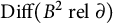 is contractible, the aforementioned map extends to
$\cup _i \Sigma _i \cup \text {\{disks\}}$
 independent of how these disks are glued in. The final step is to glue in three 3-balls, and again, the map extends, since
$\text {Diff}(B^3 \text { rel } \partial )$
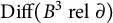 is contractible. This guarantees that we can build a diffeormophism
$Y \to Y'$
 , and moreover that the diffeomorphism preserves the trisection structure. That is, Y and
$Y'$
 are diffeomorphic as trisected 3-manifolds.
Example 2.14 Figure 4 is an example of a triple Heegaard diagram of
$T^3$
 . By noting identifications of some boundary components in
$\Sigma _1$
 and
$\Sigma _2$
 , we see that all three of
$\Sigma _1, \Sigma _2$
 and
$\Sigma _3$
 share the same
$S^1$
 boundary. Inspecting the pairs
$(\Sigma _i \cup \Sigma _{i+1}, \boldsymbol {\delta }_i)$
 , one can verify that these are cut systems on closed surfaces.
A triple Heegaard diagram of
$T^3$
 .

Figure 4: Long description
The figure consists of three panels showing topological surfaces.
Panel Sigma sub 1 (Top-Left): A complex surface with four circular openings. It features several sets of curves. Orange arcs labeled delta sub 1 span across the central body and between the openings. Teal circular curves labeled delta sub 3 wrap around the upper two openings. Small black arrows indicate orientation on the circular boundaries.
Panel Sigma sub 3 (Bottom-Left): A simpler U-shaped or open cylindrical surface with two circular ends facing the viewer. It is drawn with black outlines and no internal colored curves.
Panel Sigma sub 2 (Right): A tall, vertical bulbous surface. It is intersected by four vertical orange arcs, one of which is labeled delta sub 1. A blue horizontal circular curve labeled delta sub 2 wraps around the lower section of the surface. The top and bottom circular boundaries are marked with double-arrowheads. Dotted lines indicate the hidden back edges of the circular cross-sections.
We observe that this is a diagram of
$T^3$
 by passing through the standard genus-3 Heegaard splitting of
$T^3$
 (see [Reference Biringer, Johnson and Minsky5, Example 3.5]). The standard Heegaard splitting of
$T^3$
 has diagram
$(\Sigma _1 \cup \Sigma _2, \boldsymbol {\delta }_1, \boldsymbol {\delta }_2 \cup \boldsymbol {\delta }_3)$
 . To verify that the triple Heegaard diagram of Figure 4 builds the same 3-manifold, it suffices to observe that the cut systems
$(\Sigma _3 \cup \Sigma _1, \boldsymbol {\delta }_3)$
 and
$(\Sigma _2 \cup \Sigma _3, \boldsymbol {\delta }_2)$
 together determine the same handlebody as
$(\Sigma _1 \cup \Sigma _2, \boldsymbol {\delta }_2 \cup \boldsymbol {\delta }_3)$
 . Indeed, the two former cut systems determine handlebodies with a common disk boundary
$\Sigma _3$
 , and gluing the handlebodies along
$\Sigma _3$
 results in the handlebody determined by the latter cut system.
Example 2.15 An open book decomposition
$(\Sigma , \varphi )$
 (where
$\Sigma $
 is a page of genus g and b boundary components, and
$\varphi $
 is the monodromy) induces a trisection of the ambient 3-manifold. The trisection is represented by a
$(2g+b-1, 2g+b-1, 0, 1)$
 -triple Heegaard diagram as follows:
-
(1) The open book decomposition induces a genus $2g$
Heegaard splitting
$(\Sigma \times [0,1/2]) \cup (\Sigma \times [1/2, 1])$
, where
$\Sigma \times \{0\}$
is identified with
$\Sigma \times \{1\}$
by the monodromy map. -
(2) The Heegaard splitting is encoded by a Heegaard diagram $(\Sigma ', \boldsymbol \alpha , \boldsymbol \beta )$
which can be determined by
$\varphi $
. Reference [Reference Honda, Kazez and Matić10, Section 2] describes how to obtain such a diagram. -
(3) Let D be a disk in $\Sigma '$
disjoint from
$\boldsymbol \alpha $
and
$\boldsymbol \beta $
. Then
$(\Sigma '-D, D, D, \boldsymbol \alpha , \varnothing , \boldsymbol \beta )$
is a triple Heegaard diagram of a trisection induced by the open book decomposition. (This follows the construction in Example 2.4, and is a special case of the procedure in Example 2.14.)





A more symmetric construction is to take an open book
$(\Sigma , \varphi )$
 and immediately trisect the ambient manifold as
$(\Sigma \times [0,1/3]) \cup (\Sigma \times [1/3, 2/3]) \cup (\Sigma \times [2/3,1])$
 , again identifying
$\Sigma \times \{0\}$
 and
$\Sigma \times \{1\}$
 by the monodromy map. However, this results in a
$(2g+b-1, 2g+b-1, 2g+b-1,b)$
 -trisection, and such a trisection can be obtained by stabilizing the
$(2g+b-1,2g+b-1,0,1)$
 -trisection described above.
Remark 2.16 The data of a triple Heegaard diagram doesn’t explictly describe how the binding B is knotted—that is to say, the boundary
$B = \partial \Sigma _i$
 can be depicted in a diagram as an unlink. However, Proposition 2.13 shows that the isotopy class of the link B is nevertheless determined by triple Heegaard diagrams.
Proposition 2.17 Every 3-manifold is described by a triple Heegaard diagram.
Proof Every 3-manifold admits a trisection, as in Example 2.4. Moreover, every trisection is induced by a triple Heegaard diagram. This is because every sector of the trisection is a handlebody, and every handlebody is determined by a cut system on the boundary surface. A collection of three cut systems for each sector is precisely the data of a triple Heegaard diagram.
Example 2.18 Figure 5 depicts stabilization along a non-separating arc in
$\Sigma _1$
 . Stabilizing a diagram has three steps:
-
(1) Identify the non-separating arc $\alpha $
in some
$\Sigma _i$
along which the stabilization occurs. Thicken the arc to a band in
$\Sigma _i$
. (The thickening is unique in the sense that the framing is determined by
$\Sigma _i$
.) -
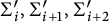
(2) The new surfaces $\Sigma _i', \Sigma _{i+1}', \Sigma _{i+2}'$
are obtained by subtracting the band in
$\Sigma _i'$
, and attaching the band to both
$\Sigma _{i+1}'$
and
$\Sigma _{i+2}'$
. -
(3) The curves on $\Sigma _i$
intersecting
$\alpha $
are cut and pasted in the new surfaces, as shown by the change from
$\delta $
to
$\delta '$
in Figure 5. A single new curve is added to
$\boldsymbol {\delta }_{i+1}$
, consisting of an arc in each band in
$\Sigma _{i+1}'$
and
$\Sigma _{i+2}'$
. This is
$\gamma $
in Figure 5, and corresponds to a meridian of the handle glued to
$Y_{i+1}$
in the stabilization.




Stabilization of triple Heegaard diagrams.

Figure 5: Long description
The diagram consists of six panels showing topological surfaces.
Top Row:
- Sigma sub 1: A curved surface featuring a thick black curve alpha and a dotted line forming a loop. An orange curve delta intersects the surface on the left.
- Sigma sub 2: A similar surface shown in outline without internal curves.
- Sigma sub 3: Identical in outline to Sigma sub 2.
Bottom Row:
- Sigma prime sub 1: The surface from Sigma sub 1 is modified with a handle-like protrusion where the alpha curve was. The orange curve is now labeled delta prime.
- Sigma prime sub 2: The surface features a handle with two small vertical segments. One is orange labeled delta prime and the other is blue. Above the handle, blue text reads gamma is an element of delta sub 2.
- Sigma prime sub 3: Similar to Sigma prime sub 2, but the handle only contains the blue vertical segment, with the same blue text gamma is an element of delta sub 2 above it.
Example 2.19 Figure 6 depicts Heegaard stabilization along an arc in
$Y_1$
 with endpoints on
$\Sigma _1$
 . It is evidently diagrammatically similar to stabilization of Heegaard splittings. In this example, since the arc has endpoints on
$\Sigma _1$
 , the sector
$Y_2$
 is unchanged while
$Y_1$
 and
$Y_3$
 increase in genus. Therefore the two new curves
$\eta $
 and
$\gamma $
 in Figure 6 belong to
$\boldsymbol {\delta }_1$
 and
$\boldsymbol {\delta }_3$
 , respectively.
Heegaard stabilization of triple Heegaard diagrams.

Figure 6: Long description
The diagram consists of two panels showing the evolution of a genus-1 surface into a genus-2 surface.
* Left Panel: A torus-like surface labeled Sigma sub 1. It features a central hole. Three nested curves are drawn on the surface. The innermost curve is teal, followed by an orange curve that wraps around the hole, and a third orange curve that extends toward the left boundary of the surface.
* Right Panel: A surface labeled Sigma prime sub 1, which has been stabilized to a genus-2 surface by adding a second handle. The left portion of the surface retains the teal and orange curves from the first panel. The new handle on the right features two intersecting curves. A teal loop labeled gamma in delta sub 3 circles the new hole horizontally. An orange loop labeled eta in delta sub 1 intersects the teal loop vertically, with a dotted line indicating the portion of the curve on the back side of the surface.
Example 2.20 Handleslides and isotopies of triple Heegaard diagrams are the same as those for Heegaard diagrams. More explicitly, given a Heegaard diagram
$(\Sigma , \boldsymbol {\alpha }, \boldsymbol {\beta })$
 , handleslide and isotopy moves are defined one handlebody at a time, i.e., on
$(\Sigma , \boldsymbol {\alpha })$
 and
$(\Sigma , \boldsymbol {\beta })$
 . In the case of a triple Heegaard diagram
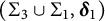
$(\Sigma _i, \boldsymbol {\delta }_i)$
 , handleslides and isotopies are defined on the pairs
$(\Sigma _1 \cup \Sigma _2, \boldsymbol {\delta }_2), (\Sigma _2 \cup \Sigma _3, \boldsymbol {\delta }_3)$
 , and
$(\Sigma _3 \cup \Sigma _1, \boldsymbol {\delta }_1)$
 .
Note that isotopies and handleslides of families of curves on
$\Sigma _i \cup \Sigma _{i+1}$
 can change how they intersect their common boundary, as shown in Figure 7.
A handleslide in the context of triple Heegaard diagrams.

Figure 7: Long description
The diagram consists of four panels showing genus-one surfaces with boundary.
Top-left panel: Labeled with the tuple (Sigma sub 1, Sigma sub 2, delta sub 1). It shows a torus-like surface with a single orange closed curve encircling the central hole.
Bottom-left panel: Shows a similar surface where the orange curve is a simple vertical loop passing through the body of the surface, indicated by a solid line on the front and a dotted line on the back.
Center: A curved arrow points from the left panels to the right panels, labeled with the word Handleslide.
Top-right panel: Labeled with the tuple (Sigma sub 1, Sigma sub 2, delta prime sub 1). The orange curve has been modified. It now originates from the left boundary, wraps around the central hole in a large loop, and returns to the left boundary, effectively sliding over the handle.
Bottom-right panel: Shows the corresponding transformation for the vertical loop. The orange curve now starts at the left boundary, travels along the length of the surface, wraps around the vertical cross-section, and returns to the left boundary.
Lemma 2.21 Fix a trisection
$(Y_1, Y_2, Y_3)$
 of a 3-manifold Y. Any two triple Heegaard diagrams
$(\Sigma _i, \boldsymbol {\delta }_i), (\Sigma _i', \boldsymbol {\delta }_i')$
 of
$(Y_1, Y_2, Y_3)$
 are diffeomorphic after a sequence of handleslides and isotopies. (That is, there are diffeomorphisms
$\varphi _i : \Sigma _i \to \Sigma _i'$
 rel boundary sending
$\boldsymbol {\delta }_i \cap \Sigma _i$
 and
$\boldsymbol {\delta }_{i-1} \cap \Sigma _i$
 to
$\boldsymbol {\delta }_i' \cap \Sigma _i$
 and
$\boldsymbol {\delta }_{i-1}' \cap \Sigma _i$
 , respectively.)
Proof Johannson [Reference Johannson11] defines a meridian-system to be a pair
$(M,\mathcal D)$
 where M is a 3-manifold with boundary and
$\mathcal D$
 is a collection of neatly embedded disks such that
$M - D$
 is homeomorphic to a 3-ball. Reference [Reference Johannson11, Corollary 1.6] shows that meridian-systems of handlebodies (which are considered up to isotopy) are unique up to handleslides. Given a sector
$Y_i$
 of the trisection,
$(\Sigma _{i}, \Sigma _{i+1}, \boldsymbol {\delta }_i)$
 induces a unique meridian-system. It follows that, up to some diffeomorphism of
$(Y_1, Y_2, Y_3)$
 , the triple Heegaard diagram is unique up to isotopy and handleslides. Finally, diffeomorphisms of the trisection descend to diffeomorphisms of triple Heegaard diagrams.
Proposition 2.22 Any two triple Heegaard diagrams of a given 3-manifold are diffeomorphic after a sequence of stabilizations, Heegaard stabilizations, handleslides, and isotopies.
Proof By Lemma 2.21, any two triple Heegaard diagrams of a fixed trisection are diffeomorphic after a sequence of handleslides and isotopies. By Proposition 2.10, any two trisections of a given 3-manifold are equivalent up to stabilization and Heegaard stabilization. (Examples 2.18 and 2.19 show how stabilization and Heegaard stabilization descend to triple Heegaard diagrams.) The result follows by applying each of these results.
Remark 2.23 Proposition 2.22 is a trisection version of the Reidemeister–Singer theorem [Reference Reidemeister21, Reference Singer22] for Heegaard splittings, which states that Heegaard diagrams of a given 3-manifold are diffeomorphic after a sequence of stabilizations, handleslides, and isotopies. (Strictly speaking the Reidemeister–Singer theorem refers to the result that Heegaard splittings are stably equivalent, but both original proofs were at the diagrammatic level.)
2.4 Complexity of 3-manifold trisections
This subsection introduces a notion of complexity for 3-manifold trisections, which will be used later to study the complexity of pseudo-trisections.
Definition 2.24 The complexity of a
$(\boldsymbol {y}, b)$
 -trisection
$\mathcal {T}$
 of a 3-manifold Y is the integer
$c(\mathcal T) = |\boldsymbol y|$
 . The minimum complexity among all trisections of Y is denoted
$c(Y)$
 .
Example 2.25 The trivial trisection of
$S^3$
 has complexity
$0$
 . It follows that
$c(S^3) = 0$
 .
Proposition 2.26 Complexity of 3-manifold trisections satisfies the following properties:
-
(1) Recalling that $p_i$
denotes the genus of the surface
$\Sigma _i$
in the trisection
$\mathcal T$
, $$ \begin{align*}c(\mathcal T) = 2|\boldsymbol p| + 3b - 3.\end{align*} $$
-
(2) Stabilization increases complexity by 1, Heegaard stabilization increases complexity by 2.
-
(3) Writing $g_H(Y)$
to denote the minimum genus of a Heegaard splitting of Y, $$ \begin{align*}c(Y) \leq 2g_H(Y).\end{align*} $$


Proof Item (1) is immediate from Proposition 2.2. Item (2) follows from earlier observations about how stabilization and Heegaard stabilization affect each
$y_i$
 . Finally item (3) follows from the fact that a genus g Heegaard splitting induces a
$(g, g, 0; 1)$
 -trisection.
Example 2.27 (Koenig [Reference Koenig12, Example 8])
The trisection of
$(S^1 \times S^2) \# (S^1 \times S^2)$
 depicted in Figure 8 has complexity
$3$
 . One can show that any trisection with complexity at most
$2$
 is necessarily induced by a Heegaard splitting of genus at most 1, and such 3-manifolds are lens spaces or
$(S^1 \times S^2)$
 . It follows that
$c((S^1 \times S^2) \# (S^1 \times S^2)) = 3$
 . Moreover,
$g_H((S^1\times S^2) \# (S^1 \times S^2)) = 2$
 , so this example shows that the inequality
$c(Y) \leq 2g_H(Y)$
 can be strict.
Triple Heegaard diagram of
$(S^1\times S^2) \# (S^1 \times S^2)$
 with complexity 3.

3 Pseudo-trisections
In this section, we introduce pseudo-trisections, which are a generalization of relative trisections of compact 4-manifolds with connected boundary. We also describe several notions of stabilization, and prove that pseudo-trisections are stably equivalent. Finally we introduce complexity of pseudo-trisections and use it to compare pseudo-trisections and relative trisections.
3.1 Pseudo-trisections and their properties
In this subsection, we define pseudo-trisections and inspect some of their properties.
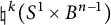
Definition 3.1 An n-dimensional 1-handlebody of genus k is a manifold with boundary diffeomorphic to
$\natural ^k (S^1 \times B^{n-1})$
 .
Definition 3.2 A
$(g, \boldsymbol {k}; \boldsymbol {y},b)$
 -pseudo-trisection of a compact connected oriented smooth 4-manifold X with one boundary component
$Y = \partial X$
 is a decomposition
$X = X_1 \cup X_2 \cup X_3$
 such that
-
(1) each $X_i$
is a 4-dimensional 1-handlebody of genus
$k_i$
, -
(2) each $H_i = X_{i-1} \cap X_i$
is a 3-dimensional 1-handlebody of genus
$h_i$
for some
$h_i$
, -
(3) each $Y_i = X_{i} \cap \partial X$
is a 3-dimensional 1-handlebody of genus
$y_i$
, -
(4) $\Sigma _C = X_1 \cap X_2 \cap X_3$
is a connected surface of genus g with b boundary components, -
(5) each $\Sigma _i = Y_{i-1} \cap Y_i$
is a connected surface of some genus
$p_i$
and b boundary components, -
(6) and $B = X_1 \cap X_2 \cap X_3 \cap \partial X$
is a b-component link.











See Figure 9 for a schematic of how the various pieces fit together.
The components of a pseudo-trisection of a 4-manifold X with boundary Y.

Figure 9: Long description
The diagram illustrates a pseudo-trisection of a 4-manifold X.
At the top, the flat circular boundary surface partial X equals Y is divided into three equal sectors meeting at a central point B.
* The top-left sector is green and labeled Y sub 3.
* The top-right sector is blue and labeled Y sub 2.
* The bottom sector is orange and labeled Y sub 1.
* The radial lines separating these sectors are labeled Sigma sub 3 (between Y sub 3 and Y sub 2), Sigma sub 2 (between Y sub 2 and Y sub 1), and Sigma sub 1 (between Y sub 1 and Y sub 3).
The interior of the hemisphere is divided into three volumes labeled X sub 1, X sub 2, and X sub 3 along the outer curved edge. These volumes are separated by internal vertical surfaces meeting at a central vertical axis labeled Sigma sub C.
* The front-left internal surface is pink and labeled H sub 3.
* The front-right internal surface is yellow and labeled H sub 2.
* The bottom-center internal surface is light blue and labeled H sub 1.
The entire manifold is labeled X on the far left.
Definition 3.3 We fix some terminology: a sector of a pseudo-trisection is any of the
$X_i$
 . The binding of a pseudo-trisection is the link B (considered as a link in
$\partial X$
 ). Finally, the 3-skeleton of a pseudo-trisection is the union of all 3-dimensional pieces,
$H_1 \cup H_2 \cup H_3 \cup \partial X$
 ; and the 2-skeleton of a pseudo-trisection is the union of all 2-dimensional pieces,
$\Sigma _C \cup \Sigma _1 \cup \Sigma _2 \cup \Sigma _3$
 . We avoid the term spine, although it is commonly used to refer to the 3-skeleta of closed 4-manifold trisections.
Proposition 3.4 Pseudo-trisections satisfy the following properties:
-
(1) The restriction of a $(g, \boldsymbol {k}, \boldsymbol {y}, b)$
-pseudo-trisection of X to
$\partial X = Y$
is a
$(\boldsymbol {y}, b)$
-trisection of Y. -
(2) The genera $p_i$
of the surfaces
$\Sigma _i$
are given by $$ \begin{align*}p_i = \tfrac{1}{2}(y_{i-1} + y_i - y_{i+1} - b + 1).\end{align*} $$
-
(3) The genera $h_i$
of the handlebodies
$H_i$
are given by $$ \begin{align*}h_i = g+p_i + b - 1 = g + \tfrac{1}{2}(y_{i-1} + y_i - y_{i+1} + b - 1).\end{align*} $$
-
(4) $\chi (X) = g - |\boldsymbol {k}| + \frac {1}{2}(|\boldsymbol {y}| + b + 1)$
.



Proof The first fact is immediate from the definition,specifically, items (3), (5), and (6) are exactly necessary properties for
$(Y_1, Y_2, Y_3)$
 to be a trisection of Y. The second fact is from Proposition 2.2, restated for completeness. The third fact follows from the fact that
$H_i$
 has boundary
$\Sigma _i \cup \Sigma _C$
 . Finally, the Euler characteristic formula is derived by repeated applications of the difference formula
$\chi (A\cup B) = \chi (A) + \chi (B) - \chi (A\cap B)$
 . Note that
$|\boldsymbol y| + b$
 is odd because
$|\boldsymbol y| + b = 2|\boldsymbol p| + 4b - 3$
 , so in each of the last three properties, no half-integers appear.
3.2 Relative trisections
Pseudo-trisections are morally generalizations of relative trisections, described in detail in [Reference A. Castro2]. We formalize the relationship between relative trisections and pseudo-trisections in Proposition 3.18. Here we review the definition of relative trisections and some fundamental results concerning relative trisections.
In order to define relative trisections, we must first fix notation for some standard model pieces—we use notation as in [Reference Gay, Pinzón-Caicedo and Castro25]. A relative trisection will then be defined in terms of these standard pieces.
Let
$g,k,p,b$
 be non-negative integers with
$g \geq p$
 and
$g+p+b-1 \geq k \geq 2p+b-1$
 . Let
$Z_k = \natural ^k S^1 \times B^3$
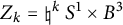 , and
$Y_k = \partial Z_k = \#^k S^1 \times S^2$
 . Next we describe a decomposition of
$Y_k$
 into three pieces, two corresponding to intersections of sectors in the relative trisection, and the other corresponding to a third of the boundary of the manifold.
Let
$D = \{(r, \theta ): r \in [0,1], \theta \in [-\pi /3, \pi /3]\}$
 . Write

where
$\partial ^- D$
 and
$\partial ^+ D$
 are the edges with
$\theta = -\pi /3$
 and
$\theta = \pi /3$
 respectively, and
$\partial ^0 D$
 is the arc. Next, let P be a surface of genus p with b boundary components, and define
$U = D \times P$
 , with

Let
$V = \natural ^{k-2p-b+1} S^1 \times B^3$
 . Notice that
$\partial V$
 has a standard Heegaard splitting. Let
$\partial V = \partial ^-V \cup \partial ^+V$
 be the splitting obtained by stabilizing the standard Heegaard splitting exactly
$g-k+p+b-1$
 times.
Since
$(k-2p-b+1) + (2p+b-1) = k$
 , there is an identification
$Z_k = U \natural V$
 . In particular, the boundary connect sum can be taken so that the decompositions of the boundaries align, giving

Definition 3.5 [Reference A. Castro2]
A
$(g,k;p,b)$
 -trisection or
$(g,k;p,b)$
 -relative trisection of a compact connected oriented 4-manifold X with connected boundary is a decomposition
$X_1 \cup X_2 \cup X_3$
 such that:
-
(1) there is a diffeomorphism $\varphi _i : X_i \to Z_k$
for each i, and -
(2) $\varphi _i(X_i \cap X_{i+1}) = Y^-_{g,k;p,b}$
,
$\varphi _i(X_i \cap X_{i-1}) = Y^+_{g,k;,p,b}$
, and
$\varphi _i(X_i \cap \partial X) = Y^0_{g,k;p,b}$
.




Remark 3.6 The indices used in the theory of relative trisections are
$(g,k;p,b)$
 , as opposed to
$(g,\boldsymbol {k}; \boldsymbol {y}, b)$
 for pseudo-trisections. First note that relative trisections as introduced here are balanced, so each of the
$k_i$
 and
$p_i$
 are independent of i. A more significant difference is that in pseudo-trisections we’ve chosen to work with
$y_i$
 rather than
$p_i$
 , that is the genera of
$Y_i$
 rather than the genera of
$\Sigma _i$
 . This is so that we can easily read off that the boundary is
$(\boldsymbol {y}, b)$
 -trisected. We also know how to convert between indices by Proposition 3.4.
Proposition 3.7 (Gay–Kirby [Reference Gay and Kirby7])
A relative trisection of a 4-manifold restricts to an open book on the boundary.
This proposition hints at a connection between relative trisections and pseudo-trisections, as we’ve shown that trisections of 3-manifolds are generalizations of open books, and pseudo-trisections restrict to 3-manifold trisections on their boundaries.
Theorem 3.8 (Castro–Islambouli–Miller–Tomova [Reference Castro, Islambouli, Miller and Tomova6])
Any two relative trisections of a given 4-manifold X are equivalent up to interior stabilizations, relative stabilizations, and relative double twists.
Proof The reader is directed to [Reference A. Castro2] for a description of relative stabilization, and a proof that any two relative trisections of 4-manifolds are equivalent up to internal and relative stabilizations, provided the induced open books on the boundary are equivalent up to Hopf stabilization. Reference [Reference Piergallini and Zuddas20, Theorem 3.5] shows that all open books of a given 3-manifold are equivalent up to Hopf stabilization and the
$\partial U$
 move (described in [Reference Piergallini and Zuddas20]). The
$\partial U$
 move is extended to the relative double twist move of relative trisections in [Reference Castro, Islambouli, Miller and Tomova6], completing the proof.
In Section 3.5, we establish the analogous result for pseudo-trisections.
Proposition 3.9 [Reference Gay, Pinzón-Caicedo and Castro25]
Every relative trisection is uniquely encoded by a relative trisection diagram. (The diagrams are unique up to handleslides and diffeomorphism.)
We do not elaborate on the definition of a relative trisection diagram, but the key takeaway is that relative trisections are encoded by diagrams of curves on a surface. We show analogously in Section 4.1 that pseudo-trisections are uniquely encoded by pseudo-trisection diagrams.
3.3
$\star $
-trisections

Another generalization of relative trisections are
$\star $
 -trisections, due to Aranda and Moeller [Reference Aranda and Moeller4]. We do not fully define them here, but the idea behind the definition is as follows:
-
(1) For each $i \in \{1,2,3\}$
, define standard 4-dimensional sectors
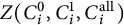
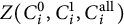
$Z(C^0_i, C^1_i, C^{\text {all}}_i)$
which depend on compression bodies
$C^{*}_i$
. These are analogous to but more general than the sectors
$Z_{k}$
introduced in the definition of relative trisections. In particular, they are typically not 4-dimensional 1-handlebodies. -
(2) A compact connected oriented 4-manifold X with connected boundary is $\star $
-trisected if there is a decomposition
$X = X_1 \cup X_2 \cup X_3$
such that each
$X_i$
is diffeomorphic to
$Z(C^0_i, C^1_i, C^{\text {all}}_i)$
, and the diffeomorphism sends pairwise intersections of the
$X_i$
s to appropriate compression bodies
$C^{*}_i$
.







The underlying motivation behind
$\star $
 -trisections is to generalize the intrisic topology of the sectors as much as possible, while maintaining a gluing theorem (which also holds for relative trisections).
Theorem 3.10 (Aranda–Moeller [Reference Aranda and Moeller4])
(Informal.) Let
$X, X'$
 be
$\star $
 -trisected 4-manifolds with boundary
$W,W'$
 . Suppose there is a homeomorphism
$f:W \to -W'$
 preserving the induced circular handle decompositions. Then the
$\star $
 -trisections on X and
$X'$
 glue to a trisection of the closed manifold
$X\cup _f X'$
 .
Conversely, the original motivation behind pseudo-trisections was to generalize the definition of relative trisections as much as possible while maintaining the intrinsic topology of the sectors. Consequently, neither pseudo-trisections nor
$\star $
 -trisections can be thought of as generalizations of one-another.
Remark 3.11 While relative trisections restrict to open books on the boundary [Reference Gay and Kirby7] and pseudo-trisections restrict to trisections on the boundary (Proposition 3.4),
$\star $
 -trisections restrict to circular handle decompositions (specifically with three thin levels, where thin levels are defined in [Reference Lamb and Weed13]) on the boundary [Reference Aranda and Moeller4]. Open books canonically induce both 3-manifold trisections and circular handle decompositions, but 3-manifold trisections do not generalize to circular handle decompositions or vice versa. (This is essentially because some 3-manifolds require arbitrarily many levels in circular handle decompositions, while trisections always exist.)
3.4 Examples of pseudo-trisections
In this subsection, we describe several examples of pseudo-trisections.
Example 3.12
The trivial trisection of
$B^4$
 . Let
$X_1, X_2, X_3$
 each be 4-balls. The boundary of each
$X_i$
 further admits the trivial trisection (in the context of 3-manifolds). We denote these sectors of
$\partial X_i$
 by
$Y_{i,j}$
 . Gluing
$X_i$
 to
$X_{i+1}$
 by identifying
$Y_{i,2}$
 and
$Y_{i+1,3}$
 produces
$B^4$
 . Explicitly, the pseudo-trisection consists of:
-
• $X_1, X_2, X_3$
as described, -
• $H_i = Y_{i-1,2} = Y_{i,3}$
, -
• $Y_i = Y_{i, 1}$
,



and the lower dimensional pieces are obtained by appropriate intersections. Note that this is also a relative trisection.
Example 3.13
A pseudo-trisection of
$B^3\times S^1$
 which is not a relative trisection. Let
$X_1, X_2 = B^3 \times S^1$
 , and
$X_3 = B^4$
 .
$X_1$
 and
$X_2$
 have boundary
$S^2 \times S^1$
 . Consider the trisection of
$S^2 \times S^1$
 induced by its genus 1 Heegaard splitting, as well as the standard trisection of
$S^3$
 . We denote these sectors by
$Y_{i,j}$
 , where
$Y_{1,1}, Y_{1,2}, Y_{2,1}, Y_{2,3}$
 are solid tori, and
$Y_{1,3}$
 and
$Y_{2,2}$
 are solid balls. Let
$Y_{3,j}$
 be the sectors of the trivial trisection of the boundary of
$X_3$
 .
We claim that gluing
$X_i$
 to
$X_{i+1}$
 by identifying
$Y_{i,2}$
 and
$Y_{i+1, 3}$
 produces
$B^3 \times S^1$
 . To see this, observe that
$X_1$
 and
$X_2$
 are glued along a copy of
$D^2 \times S^1$
 in their boundaries. This is a boundary connected sum in the first entry, so the resulting manifold is still
$B^3 \times S^1$
 . Next,
$X_3$
 is glued to
$X_1 \cup X_3$
 along two 3-balls, but these two 3-balls also meet along a disk. The result is another boundary connected sum. It follows that the resulting manifold is
$B^3 \times S^1$
 .
The sectors of the pseudo-trisection are all labeled consistently with Example 3.12. See Figure 10 for a schematic of the pseudo-trisection. Note that this pseudo-trisection is not a relative trisection because the boundary doesn’t inherit an open book structure.
A schematic of how the sectors are glued together in Example 3.13.

Figure 10: Long description
The diagram consists of three main objects labeled X sub 2, X sub 1, and X sub 3 from left to right.
* Object X sub 2 on the left is a torus with a blue outer face labeled Y sub 2 = Y sub 2,1 and a yellow inner face. A pink circular sector is embedded on its right side.
* Object X sub 1 in the center is a torus with a yellow outer face and an orange inner face labeled Y sub 1 = Y sub 1,1. A blue circular sector is embedded on its right side.
* Object X sub 3 on the bottom right is a sphere divided into three colored sectors: pink, green, and blue. The sphere is labeled X sub 3 and its primary surface is Y sub 3 = Y sub 3,1.
Three sets of curved bidirectional arrows indicate gluing maps between the objects:
* An arrow at the top connects the pink sector of X sub 2 (labeled Y sub 2,3) to the yellow face of X sub 1 (labeled Y sub 1,2).
* An arrow in the middle connects the blue sector of X sub 1 (labeled Y sub 1,3) to the blue sector of X sub 3 (labeled Y sub 3,2).
* An arrow at the bottom connects the yellow face of X sub 2 (labeled Y sub 2,2) to the pink sector of X sub 3 (labeled Y sub 3,3).
Example 3.14
A pseudo-trisection of
$B^2 \times S^2$
 which is not a relative trisection. Let each of
$X_1,X_2,X_3$
 be a 4-ball. Writing
$X_1$
 and
$X_2$
 as
$B^2 \times B^2$
 , the genus 1 Heegaard splittings of their boundaries can be written as
$(S^1 \times B^2)\cup (B^2 \times S^1)$
 . These induce trisections


In the above descriptions, B is a ball removed from a sector of the Heegaard splitting to produce a trisection, as described in Example 2.4. Let the boundary of
$X_3$
 be a trivially trisected
$S^3$
 as in Example 3.13.
Gluing the three sectors as in Examples 3.12 and 3.13, we obtain a pseudo-trisection of
$B^2 \times S^2$
 . To see this, notice that
$X_1$
 and
$X_2$
 are two copies of
$B^2 \times B^2$
 being glued along
$B^2 \times S^1$
 , which produces
$B^2 \times S^2$
 . As in the previous example, gluing
$X_3$
 does not alter the topology. Again, the sectors are labeled consistently with previous examples.
Example 3.15
A pseudo-trisection of
$\mathbb {CP}^2 - B^4$
 . There is a standard genus 1 trisection
$\mathcal T$
 of
$\mathbb {CP}^2$
 as seen for example in [Reference Gay and Kirby7]. A neighborhood of a point in the central surface of
$\mathcal T$
 is a trivially trisected
$B^4$
 . Removing this ball produces a relative trisection of
$\mathbb {CP}^2 - B^4$
 (which is also a pseudo-trisection).
Example 3.16 Given pseudo-trisections
$(X_1,\mathcal {T}_1)$
 and
$(X_2,\mathcal {T}_2)$
 , there are pseudo-trisections of the form
$\mathcal {T}_1\natural \mathcal {T}_2$
 on
$X_1\natural X_2$
 . These are called boundary connected sums of the pseudo-trisections, and restrict to a connected sum of the boundary trisections as described in Example 2.5. These are not unique—there are generally
$3b_1 b_2$
 distinct boundary connected sums, where
$b_1$
 and
$b_2$
 are the number of components of the bindings of
$\mathcal {T}_1$
 and
$\mathcal {T}_2$
 , respectively.
Explicitly, we build the boundary connected sum as follows:
-
(1) Choose points $q_1$
and
$q_2$
in the bindings
$B_1$
and
$B_2$
of
$\mathcal {T}_1$
and
$\mathcal {T}_2$
respectively. These each have standard neighborhoods
$N(q_1), N(q_2)$
in their respective pseudo-trisections, diffeomorphic to the trivial trisection. Let
$M(q_1)$
and
$M(q_2)$
denote the restriction of these neighborhoods to
$\partial X_1$
and
$\partial X_2$
. Note that we have made one of
$b_1 b_2$
choices in specifying
$q_1$
and
$q_2$
. -
(2) The neighborhoods $M(q_1)$
and
$M(q_2)$
are trivially trisected in the sense that each is a 3-ball with an induced decomposition into three 3-balls, pairwise meeting along disks, with total-intersection an arc. These inherit labels
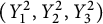
$(Y_1^1, Y_2^1, Y_3^1)$
and
$(Y_{1}^2, Y_2^2, Y_3^2)$
, respectively. We take the boundary connected sum of
$X_1$
and
$X_2$
by identifying
$M(q_1)$
with
$M(q_2)$
while further respecting the decompositions of the balls into sectors. -
(3) There are three choices we can make, since the identification can send $Y_1^1$
to any one of
$Y_{i}^2$
, and this determines the rest of the identification. In total, this means we have built one of
$3b_1 b_2$
possible boundary connected sums.







Remark 3.17 The boundary connected sum of pseudo-trisections is distinct from the plumbing of relative trisections by Murasugi sum described in [Reference Castro, Islambouli, Miller and Tomova6, Theorem 3.20]. Specifically, a boundary connected sum of two relative trisections will generally not be a relative trisection.
Proposition 3.18 A relative trisection of a 4-manifold with one boundary component is a pseudo-trisection, provided the binding of the induced open book on the boundary is non-empty.
Proof It must be shown that relative trisections as above satisfy all six of the defining properties of pseudo-trisections from Definition 3.2. Property 1 is immediate, since the definition of relative trisections requires that each sector
$X_i$
 is diffeomorphic to a standard piece
$Z_k$
 . Properties 4, 5, and 6 are exactly observations 1, 2, and 3 at the start of [Reference Gay, Pinzón-Caicedo and Castro24, Section 4]. This leaves properties 2 and 3.
In a relative trisection,
$H_i = X_i \cap X_{i-1}$
 is necessarily diffeomorphic to a standard piece
$Y^+_{g,k;p,b}$
 . This is a compression body from
$\Sigma _{g,b}$
 to
$\Sigma _{p,b}$
 obtained by compressing along
$g-p$
 simple closed curves. In the proposition statement, we require that the binding of the induced open book in the boundary is non-empty, which is equivalent to requiring that b is at least 1. A compression body of this form is diffeomorphic to a handlebody of genus
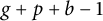
$g+p+b-1$
 , verifying that property 2 is satisfied.
Finally we must verify that property 3 is satisfied. In the notation of [Reference Gay, Pinzón-Caicedo and Castro24], we have that
$X_i \cap \partial X$
 is diffeomorphic to a standard piece
$Y^0_{g,k;p,b}$
 , which is itself equal to
$(D \times \partial \Sigma _{p,b}) \cup (I \times \Sigma _{p,b})$
 , where D is a wedge of a disk and I is the intersection of D with the boundary of the underlying disk. Topologically the union corresponds to gluing b solid tori to
$I \times \Sigma _{p,b}$
 along their longitudes, and thus
$Y^0_{g,k;p,b}$
 is diffeomorphic to
$I \times \Sigma _{p,b}$
 . Again since
$b \geq 1$
 , the latter is a handlebody (of genus
$2p+b-1$
 ).
Remark 3.19 The restriction to
$(g,k,p,b)$
 -relative-trisections with
$b\geq 1$
 is not a strict condition. Firstly, any relative trisection can be Hopf-stabilized [Reference A. Castro2] to increase b. Secondly, the usual recipe to construct a relative trisection is to first fix an open book on the boundary 3-manifold, and this open book can be chosen to have non-empty binding.
Corollary 3.20 Every compact connected oriented smooth 4-manifold with connected boundary admits a pseudo-trisection.
Proof Every such 4-manifold admits a relative trisection [Reference A. Castro2]. In particular, the binding can be chosen to be non-empty. This relative trisection is a pseudo-trisection.
3.5 Stabilizations and uniqueness of pseudo-trisections
We recall internal stabilization, and introduce two more notions of stabilizations of pseudo-trisections supported near the boundary. We then show that any pseudo-trisections of a given compact 4-manifold with connected boundary are equivalent under these three notions of stabilization.
In [Reference A. Castro2], it is shown that relative trisections of a given 4-manifold with boundary X are stably equivalent, provided their boundaries are stably equivalent. More precisely, two notions of stabilization are used: internal stabilization, which doesn’t affect the open book on the boundary, and Hopf stabilization which stabilizes the open book in the boundary by adding a Hopf band. However, not all open books of a given 3-manifold are equivalent under Hopf stabilization.
In the context of pseudo-trisections, the boundary 3-manifold is equipped with a trisection rather than an open book, and all trisections of a given 3-manifold are related by appropriate notions of stabilization. This allows us to define a set of moves so that for any given 4-manifold, all pseudo-trisections of the manifold are stably equivalent, without conditioning over the boundary.
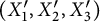
Definition 3.21 Given a pseudo-trisection
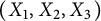
$(X_1, X_2, X_3)$
 of a 4-manifold X, an internal stabilization is a new pseudo-trisection
$(X_1', X_2', X_3')$
 of X constructed as follows:
-
(1) Choose a neatly embedded boundary parallel arc $\alpha $
in
$H_i = X_i \cap X_{i-1}$
for some i, with endpoints on
$\Sigma _C = X_1 \cap X_2 \cap X_3$
. -
(2) Let $N(\alpha )$
be a tubular neighborhood of
$\alpha $
in X supported away from
$\partial X$
, and define-
• $X_{i+1}' = X_{i+1} \cup \overline {N(\alpha )}$
, -
• $X_{i}' = X_i - N(\alpha )$
, -
• $X_{i-1}' = X_{i-1} - N(\alpha )$
.
-








See Figure 11 (left) for a schematic of internal stabilization.
From left to right: schematics of internal stabilization, boundary stabilization, and Heegaard stabilization.

Figure 11: Long description
A three-panel diagram showing topological stabilization on a hemisphere divided into colored sectors.
In the first panel on the left, representing internal stabilization, a curved, tube-like handle is added entirely within the interior of the hemisphere, connecting two points on an internal vertical boundary between the pink and yellow sectors.
In the middle panel, representing boundary stabilization, a handle is added to the top flat surface of the hemisphere. It forms a bridge over the intersection of the green, blue, and orange sectors, creating a new hole on the boundary surface.
In the third panel on the right, representing Heegaard stabilization, a handle is integrated into the boundary between the blue and orange sectors. It appears as a localized protrusion and indentation that modifies the intersection of the surface regions.
Each hemisphere uses a consistent color scheme of green, blue, and orange on the top surface, and pink, light blue, and yellow on the curved lower surface, with dotted lines indicating internal partitions.
Notice that stabilization increases the handlebody genus
$k_{i+1}$
 of
$X_{i+1}$
 by 1, while leaving
$k_i$
 and
$k_{i-1}$
 unchanged. The genus g of
$\Sigma _C$
 also increases by 1. This move is essentially “one third” of the usual notion of stabilization for balanced trisections of closed 4-manifolds.
Definition 3.22 Given a pseudo-trisection
$(X_1, X_2, X_3)$
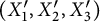
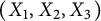 of a 4-manifold X with boundary Y, a boundary stabilization is a new pseudo-trisection
$(X_1', X_2', X_3')$
 of X constructed as follows:
-
(1) Choose a neatly embedded non-separating arc $\alpha $
in
$\Sigma _i$
. (Such an arc exists provided
$\Sigma _i$
is not a disk.) -
(2) Let $N(\alpha )$
be a tubular neighborhood of
$\alpha $
in X, and define-
• $X_{i+1}' = X_{i+1} \cup \overline {N(\alpha )}$
, -
• $X_{i}' = X_i - N(\alpha )$
, -
• $X_{i-1}' = X_{i-1} - N(\alpha )$
.
-





See Figure 11 (middle) for a schematic of boundary stabilization.
The definition looks very similar to that of internal stabilization—one way to differentiate them is that internal stabilization is defined with an arc
$\alpha $
 in
$H_i$
 that is far from
$\Sigma _i = H_i \cap \partial X$
 , while boundary stabilization is defined with an arc
$\alpha $
 that lives entirely in
$\partial X$
 .
We make the following observations:
-
(1) The restriction of $N(\alpha )$
to Y is a tubular neighborhood of
$\alpha $
in Y. Therefore the restriction of
$(X_1', X_2', X_3')$
to Y is a stabilization (in the sense of Definition 2.6) of the restriction of
$(X_1, X_2, X_3)$
to Y. (More succinctly, the restriction of a boundary stabilization is a 3-manifold stabilization of the restriction.) In particular, if
$(X_1, X_2, X_3)$
was a
$(g, \boldsymbol k; \boldsymbol y, b)$
-pseudo-trisection of X, then in the stabilization
$\boldsymbol y$
and b change as described in Section 2.1. -
(2) The genera $\boldsymbol k$
of the 4-dimensional sectors change in the same way as
$\boldsymbol y$
. That is,
$k_{i+1}$
increases by 1, while
$k_i$
and
$k_{i-1}$
are unchanged. -
(3) The genus g of $\Sigma _C$
increases by 1 if the endpoints of
$\alpha $
lie in different components of B, and is unchanged if the endpoints of
$\alpha $
lie in the same component. This can be seen directly, as boundary stabilization descends to a band attachment on
$\Sigma _C$
, but it can also be deduced using the Euler characteristic formula for pseudo-trisections in Proposition 3.4.


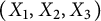
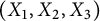


Definition 3.23 Given a pseudo-trisection
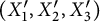
$(X_1, X_2, X_3)$
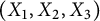 of a 4-manifold X with boundary Y, a Heegaard stabilization is a new pseudo-trisection
$(X_1', X_2', X_3')$
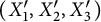 of X constructed as follows:
-
(1) Choose a neatly embedded boundary parallel arc $\alpha $
in
$Y_i = X_i \cap \partial X$
for some i, with both endpoints on
$\Sigma _i$
. -
(2) Let $N(\alpha )$
be a tubular neighborhood of
$\alpha $
in
$X_i$
, and define-
• $X_{i+1}' = X_{i+1}$
, -
• $X_i' = X_i - N(\alpha )$
, -
• $X_{i-1}' = X_{i-1} \cup \overline {N(\alpha )}$
.
-






See Figure 11 (right) for a schematic of Heegaard stabilization.
We make the following observations:
-
(1) Analogously to boundary stabilizations restricting to stabiliations of the boundary, a Heegaard stabilization of a pseudo-trisection restricts to a Heegaard stabilization of the 3-manifold trisection of the boundary Y. In particular, a Heegaard stabilization of a pseudo-trisection changes $y_i$
and
$y_i-1$
by 1, while leaving
$y_{i+1}$
and b unchanged. -
(2) The sector $X_{i-1}$
gains a 1-handle in the stabilization, so
$k_{i-1}$
increases by 1. On the other hand,
$N(\alpha )$
being carved out of
$X_{i}$
does not change the topology of
$X_{i}$
, since
$N(\alpha )$
runs along the boundary of
$X_{i}$
. Therefore
$k_{i}$
and
$k_{i+1}$
are unchanged. -
(3) The central surface $\Sigma _C$
is unchanged, so b is unchanged. One can verify that all of these index changes are compatible with the Euler characteristic formula.


Internal stabilization and Heegaard stabilization are unified into the single notion of torus stabilization at the diagrammatic level, introduced later in Definition 4.7.
Theorem 1.2 Let X be a compact connected oriented smooth 4-manifold with one boundary component. Any two pseudo-trisections of X are equivalent up to internal, boundary, and Heegaard stabilization.
Proof There are two steps: first we stabilize the pseudo trisections to agree on the boundary, and then stabilize the interior.
Let
$\mathcal T, \mathcal T'$
 be pseudo-trisections of X. Their restrictions
$\tau , \tau '$
 to
$Y = \partial X$
 are trisections of Y. By Proposition 2.10,
$\tau $
 and
$\tau '$
 are stably equivalent. This means there is a trisection
$\sigma $
 of Y and arcs
$\{\alpha \}, \{\alpha '\}$
 such that stabilizations and Heegaard stabilizations of
$\tau $
 along
$\{\alpha \}$
 produces
$\sigma $
 , and similarly stabilizations and Heegaard stabilizations of
$\tau '$
 along
$\{\alpha '\}$
 produces
$\sigma $
 .
We now return to 4-dimensions: Boundary stabilizing and Heegaard stabilizing
$\mathcal T$
 along
$\{\alpha \}$
 produces a pseudo-trisection
$\mathcal S$
 which restricts to the 3-manifold trisection
$\sigma $
 on Y. On the other hand, boundary and Heegaard stabilizing
$\mathcal T'$
 along
$\{\alpha '\}$
 produces a pseudo-trisection
$\mathcal S'$
 which also restricts to
$\sigma $
 on Y. We have successfully stabilized our pseudo-trisections to agree on the boundary.
Next we turn to the interior. We proceed as in the proof of the analogous result for closed trisections in [Reference Gay and Kirby7]. To that end, we require a cobordism structure on X, which we obtain by first turning our boundary trisection into a Heegaard splitting.
Consider the sectors
$X_1$
 and
$X_1'$
 in
$\mathcal S$
 and
$\mathcal S'$
 respectively. These restrict to
$Y_1 = Y_1'$
 on the boundary. Choose a maximal collection of non-separating arcs in
$\Sigma _3$
 . Boundary stabilizing the two pseudo-trisections along these arcs produces two new pseudo-trisections (which we still call
$\mathcal S$
 and
$\mathcal S'$
 ). However, the restricted trisection on the boundary now has that
$\Sigma _3$
 is a disk. This means
$Y_{2}\cup Y_{3}$
 now glues along a disk, so it is itself a handlebody. In summary, the decomposition
$Y_{1} \cup (Y_{2} \cup Y_{3})$
 is a Heegaard splitting.
Next we view X as a cobordism from
$Y_{2} \cup Y_{3}$
 to
$Y_{1}$
 . Formally, we do this by considering a tubular neighborhood N of the Heegaard splitting surface
$\Sigma _{1}\cup \Sigma _{2}$
 , so that Y is of the form
$(Y_1-N) \cup N \cup (Y_2 \cup Y_3 - N)$
 . The theorem now essentially follows from [Reference Gay and Kirby7, Theorem 21]: there are relative handle decompositions (equivalently, Morse functions), induced by the pseudo-trisections and compatible with the cobordism structure. Cerf theory tells us that the handle decompositions are related by a series of moves which correspond to internal stabilization. In summary, after a sequence of internal stabilizations, our pseudo-trisections are isotopic.
Remark 3.24 The proof of Theorem 1.2 doesn’t involve Heegaard stabilization unless one of the original trisections of X restricts to the trivial open book on Y. For example, if the boundary of X is not a sphere, the above theorem holds using only boundary and internal stabilizations.
3.6 Complexity of pseudo-trisections and relative trisections
This subsection introduces a notion of complexity for pseudo-trisections, which also applies to relative trisections. It can be considered a generalization of the genus of a trisection (of a closed manifold). We show that each notion of stabilization increases complexity by 1. The minimal complexity of a pseudo-trisection of a given 4-manifold with boundary is bounded above by the minimal complexity of a relative trisection (since relative trisections are pseudo-trisections), but we see with some examples that these minimal complexities do not generally agree.
Definition 3.25 The complexity of a
$(g,\boldsymbol {k},\boldsymbol {y},b)$
 -pseudo-trisection
$\mathcal {T}$
 of a 4-manifold X with boundary
$\partial X$
 is the integer

Further, we write
$c(\partial \mathcal T)$
 to denote the complexity of the induced trisection on
$\partial X$
 , and
$c(\mathcal T, \partial \mathcal T)$
 to denote
$c(\mathcal T) + c(\partial \mathcal T)$
 . We write
$c(X)$
 to denote the minimum complexity among all pseudo-trisections of X, and
$c(X,\partial X)$
 to denote the minimum value of
$c(\mathcal T, \partial \mathcal T)$
 among all pseudo-trisections of X.
Remark 3.26 It is immediate that
$c(X,\partial X)$
 is at least
$c(X) + c(\partial X)$
 , but it is not known whether or not they are always equal.
Proposition 3.27 Complexity satisfies the following properties:
-
(1) Recalling that $p_i$
denotes the genus of the surface
$\Sigma _i$
of the pseudo-trisection, $$ \begin{align*}c(\mathcal{T}) = g + \frac{1}{2}(|\boldsymbol{y}| + b - 1) = g + |\boldsymbol{p}| + 2b - 2.\end{align*} $$
-
(2) The three types of stabilization for pseudo-trisections increase complexity by 1.
-
(3) Write $\beta _i$
for the Betti numbers of X.-
(a) For $\mathcal {T}$
a relative trisection,
$c(\mathcal {T}) \geq \beta _1 + \beta _2$
. -
(b) For $\mathcal {T}$
a pseudo-trisection,
$c(\mathcal {T},\partial \mathcal {T})\geq \beta _1 + \beta _2$
.
-
-
(4) Given pseudo-trisected manifolds $(X_1, \mathcal {T}_1)$
,
$(X_2,\mathcal {T}_2)$
, complexity is additive in the sense that
$c(\mathcal {T}_1 \natural \mathcal {T}_2) = c(\mathcal {T}_1) + c(\mathcal {T}_2)$
.








Proof In item (1), the first equality is an application of the last item in Proposition 3.4. The second equality is an application of the second item in the aforementioned proposition.
For item (2), we use the observation that each of the three types of stabilization for pseudo-trisections increases one of the
$k_i$
 by 1, while leaving the other two unchanged.
For item (3), we require several steps. In step 1, we establish a general homological statement about 4-manifolds with boundary. In step 2 we establish bounds for
$\beta _1$
 in terms of
$|\boldsymbol {k}|$
 (and
$|\boldsymbol {y}|$
 ) for relative trisections (and pseudo-trisections).
Step 1. In the long exact sequence
$H_4(X,\partial X) \xrightarrow {i} H_3(\partial X) \xrightarrow {j} H_3(X) \xrightarrow {k} H_3(X,\partial X)$
 , the map k is necessarily injective because i is an isomorphism. Combining this fact with the isomorphism
$H^1(X) \cong H_3(X,\partial X)$
 , we have

On the other hand,
$\chi (X) = 1 - \beta _1 + \beta _2 - \beta _3$
 , so

Step 2. Suppose
$\mathcal {T}$
 is either a relative trisection or pseudo-trisection. Let
$\gamma $
 be a neatly embedded loop in X. Then
$\gamma $
 meets each
$X_i$
 along a set of arcs whose endpoints lie in
$\partial X_i$
 . Since each
$X_i$
 is a handlebody, the arcs can be homotoped rel boundary to lie in
$\partial X_i$
 . We do this in every sector, to obtain a loop
$\gamma '$
 contained entirely within the 3-skeleton of
$\mathcal {T}$
 . Next we repeat this step a dimension lower:
$\gamma '$
 intersects each
$H_i$
 or
$Y_i$
 along an arc with endpoints in
$\partial H_i$
 or
$\partial Y_i$
 respectively. These arcs can again be homotoped rel boundary to lie within
$\partial H_i$
 and
$\partial Y_i$
 respectively. Doing this in every 3-dimensional sector, we obtain a loop
$\gamma "$
 contained entirely within the 2-skeleton of
$\mathcal {T}$
 .
The proof now diverges for pseudo-trisections and relative trisections. In the former case, notice that
$\gamma "$
 can be viewed as loop in
$X_i \cup \Sigma _{i-1}$
 for any i. This means
$\pi _1(X_i \cup \Sigma _{i-1})$
 surjects onto
$\pi _1(X)$
 . Taking into account how
$\Sigma _{i-1}$
 is glued to
$X_i$
 , it follows that
$2p_{i-1} + b - 1 + k_i \geq \beta _1$
 . This holds over each i, giving

Combining this with the result from step 1 gives

In the case of relative trisections, the boundary is an open book. Therefore the arcs
$\gamma " \cap \Sigma _i$
 can be homotoped rel boundary to any
$\Sigma _j$
 via the fibration defining the open book. It follows that
$\gamma "$
 can be homotoped to lie entirely within any one of the
$X_i$
 . It follows that
$|\boldsymbol {k}| \geq 3\beta _1$
 , and therefore that
$c(\mathcal {T}) \geq \beta _1 + \beta _2$
 .
Finally, for item (4), we have that

as required.
Remark 3.28 Proposition 3.27 implies that
$c(X_1\natural X_2) \leq c(X_1) + c(X_2)$
 . It is not known if this inequality is ever strict. This is analogous to the question of whether or not trisection genus is additive under connected sum.
Example 3.29 Figure 12 lists the minimum complexities of some relative trisections and pseudo-trisections. It demonstrates that even for simple 4-manifolds complexities of relative trisections tend to be much greater than the lower bound given in Proposition 3.27. On the other hand, complexities of pseudo-trisections appear to be equal to
$\beta _1 + \beta _2$
 . This suggests that relative trisections tend to have significantly higher complexity than pseudo-trisections.
The five (minimal) pseudo-trisections in Figure 12 are presented in Examples 3.12, 3.13, 3.14, and 3.15 and below in Figure 13. Since any pseudo-trisection with complexity
$0$
 is the trivial pseudo-trisection, it is automatic that the given pseudo-trisections for
$S^1\times B^3$
 and
$S^2\times D^2$
 must be minimal. Next, one can see that any pseudo-trisection with complexity
$1$
 must have boundary a lens space or
$S^1\times S^2$
 . It follows that the given pseudo-trisection for
$(S^2\times D^2)\natural (S^2\times D^2)$
 is also minimal. Another minimal pseudo-trisection of
$(S^2\times D^2)\natural (S^2\times D^2)$
 is given by the boundary connected sum of a complexity 1 pseudo-trisection with itself.
Complexities of some simple 4-manifolds. When not known, the interval of possibilities is written.

Figure 12: Long description
The table consists of six rows and five columns.
Column headers from left to right are:
1. Manifold type (unlabeled header)
2. beta sub 1 plus beta sub 2
3. Rel.-T. c(X)
4. Pseudo-T. c(X)
5. Pseudo-T. c(X, partial X)
Data rows from top to bottom:
- B super 4: 0, 0, 0, 0.
- C P super 2 minus B super 4: 1, 1, 1, 1.
- S super 1 times B super 3: 1, 2, 1, 3.
- S super 2 times D super 2: 1, the interval [3,4], 1, 3.
- (S super 2 times D super 2) connected sum (S super 2 times D super 2): 2, the interval [4,8], 2, 5.
A pseudo-trisection diagram of
$(S^2\times D^2) \natural (S^2\times D^2)$
 .

Figure 13: Long description
The diagram consists of four panels, each depicting a horizontal cylinder with specific internal curves.
* Top-left panel labeled Sigma sub 1. A light blue horizontal line alpha sub 1 runs along the top of the cylinder. An orange vertical circle delta sub 1 wraps around the center of the cylinder.
* Top-right panel labeled Sigma sub 2. A yellow horizontal line alpha sub 2 runs through the center of the cylinder. A dark blue vertical circle delta sub 2 wraps around the center.
* Bottom-left panel labeled Sigma sub 3. A pink horizontal line alpha sub 3 runs along the bottom of the cylinder. A green vertical circle delta sub 3 wraps around the center.
* Bottom-right panel labeled Sigma sub C. This cylinder contains all three horizontal lines from the previous panels: the light blue alpha sub 1 at the top, the yellow alpha sub 2 in the center, and the pink alpha sub 3 at the bottom. It does not contain any vertical circles.
In all panels, the left end of the cylinder is marked with a dotted elliptical curve, and the right end is a solid elliptical curve.
For relative trisections, it is again clear that the trivial trisection of
$B^4$
 is minimal, and any other trisection has complexity at least
$1$
 . Therefore the relative trisection given in Example 3.15 is minimal. Any relative trisection with complexity
$1$
 must have boundary
$S^3$
 . It follows that a relative trisection of
$S^1\times B^3$
 with complexity
$2$
 would be minimal. Such a relative trisection exists—it is prescribed by the relative trisection diagram consisting of an annulus (and no curves). Moreover, this is the only relative trisection with complexity
$2$
 and boundary not a sphere, as can be seen by enumerating diagrams.
From here, it follows that any relative trisection of
$S^2\times D^2$
 with complexity 3 must be minimal. However, the author could not find such an example, or rule out its existence. To the author’s best knowledge, the smallest known relative trisection of
$S^2\times D^2$
 has complexity 4—see [Reference A. Castro and Ozbagci3, Example 2.9].
Finally, one can show again by enumerating diagrams that any relative trisection of
$(S^2\times D^2) \natural (S^2\times D^2)$
 must have complexity at least
$4$
 . To the author’s best knowledge, the smallest known relative trisection of
$(S^2\times D^2)\natural (S^2\times D^2)$
 has complexity 8, by taking the “plumbing” of a relative trisection of
$S^2\times D^2$
 with itself (in the sense of [Reference Castro, Islambouli, Miller and Tomova6, Theorem 3.20]). Note that it is not known whether or not relative trisection genus (equivalently, complexity) is additive under boundary connected sum [1].
Example 3.30 For pseudo-trisections,
$c(\natural ^\ell (S^2\times D^2)) \leq \ell $
 . This is because we can iteratively take the boundary connected sum of the complexity 1 pseudo-trisection in Example 3.14 with itself, and complexity is subadditive. On the other hand, restricting to relative trisections and assuming additivity of relative trisection genus,
$c(\natural ^\ell (S^2\times D^2)) \geq 3\ell $
 by Example 3.29.
Remark 3.31 In Examples 3.29 and 3.30, we reference the question of whether or not relative trisection genus is additive under boundary connected sum. Evidence for the additivity of relative trisection genus is presented in a recent preprint of Takahashi [Reference Takahashi26]. Note that additivity of relative trisection genus would imply additivity of (closed) trisection genus, which in turn implies the Smooth Poincaré conjecture in dimension 4 [Reference Lambert-Cole and Meier14].
Remark 3.32 The author is unaware of manifolds X for which
$c(X) < \beta _1 + \beta _2$
 or
$c(X,\partial X) = \beta _1 + \beta _2, c(\partial X)> 0$
 . It appears likely that the bound given in Proposition 3.27 for pseudo-trisections can be improved.
Remark 3.33 To better measure the extent to which pseudo-trisections have lower complexity than relative trisections, we would need a sufficiently tight upper bound on the complexity of pseudo-trisections. This corresponds to further refining existence results in a way which is not done here.
3.7 Classification of low complexity pseudo-trisections
In this subsection, we determine which 4-manifolds admit pseudo-trisections with complexity at most 1. Consequently, we show that additivity of pseudo-trisection complexity under boundary connected sum would imply that disk bundles over
$S^2$
 are standard. We start by recalling a similar result in the closed setting.
Proposition 3.34 (Meier–Lambert–Cole, [Reference Lambert-Cole and Meier14, Proposition 1.7])
If trisection genus is additive under connected sum, then there is no exotic
$S^4, \mathbb {CP}^2, S^1\times S^3, S^2\times S^2, \mathbb {CP}^2\#\mathbb {CP}^2$
 , nor
$\mathbb {CP}^2\# \overline {\mathbb {CP}}{}^2$
 .
If trisection genus is additive, a theorem of Wall [Reference Wall27] implies that trisection genus is a homeomorphism invariant of smooth manifolds. It remains to classify the closed 4-manifolds of given trisection genera, and indeed the above list corresponds to those with trisection genera at most 2.
Proposition 3.35 Let X be a compact connected oriented smooth 4-manifold with one boundary component.
-
• If $c(X) = 0$
, then X is
$B^4$
. Conversely,
$B^4$
admits a unique pseudo-trisection up to diffeomorphism with complexity 0. -
• If $c(X) = 1$
, then X is either
$B^4, \mathbb {CP}^2 - B^4, S^1 \times B^3$
, or a disk bundle over
$S^2$
. Conversely, each of these manifolds admits a unique pseudo-trisection up to diffeomorphism with complexity 1.




Proof The proof structure is to determine all possible pseudo-trisection diagrams with complexity 0 or 1 up to handleslides and isotopies. This proof depends on Section 4 and in particular Lemma 4.6, but we have placed it here for thematic reasons.
It is immediate that a pseudo-trisection with complexity
$0$
 is the trivial pseudo-trisection.
Next, suppose X is pseudo-trisected with complexity
$1$
 . By Proposition 3.27,
$b=1$
 is fixed, and exactly one of
$\Sigma _C, \Sigma _1, \Sigma _2, \Sigma _3$
 has genus 1 while the rest are disks.
Case 1:
$\Sigma _C$
 has genus 1, and each
$\Sigma _i$
 is a disk. Then identifying the boundary of X with the boundary of a trivially trisected
$B^4$
 produces a trisection of a closed manifold with trisection genus 1. By [Reference Gay and Kirby7] this trisection is the unique trisection of
$\mathbb {CP}^2$
 up to diffeomorphism, and consequently X is
$\mathbb {CP}^2 - B^4$
 , also trisected up to diffeomorphism with complexity
$1$
 .
Case 2: Without loss of generality,
$\Sigma _1$
 has genus 1, and each of
$\Sigma _C, \Sigma _2, \Sigma _3$
 is a disk. Then there is a pseudo-trisection diagram of the pseudo-trisection of X consisting of three simple closed curves
$\alpha _1, \delta _1, \delta _3$
 on
$\Sigma _1$
 . The triple Heegaard diagrams
$(\Sigma _C, \Sigma _3,\Sigma _1,\varnothing , \delta _3,\alpha _1)$
 and
$(\Sigma _C, \Sigma _1, \Sigma _2, \alpha _1, \delta _1, \varnothing )$
 must encode either
$S^3$
 or
$S^1\times S^2$
 , which corresponds to the intersection numbers
$\alpha _1 \cdot \delta _1$
 and
$\delta _3 \cdot \alpha _1$
 being
$0$
 or
$1$
 .
Suppose
$\alpha _1 \cdot \delta _1 = 0$
 and
$\delta _3 \cdot \alpha _1 = 0$
 . Then the resulting pseudo-trisection is of
$S^1\times B^3$
 , described in Example 3.13. Suppose
$\alpha _1\cdot \delta _1 = 0$
 and
$\delta _3 \cdot \alpha _1 = 1$
 . Then
$\delta _3 \cdot \delta _1 = 1$
 , and the resulting trisection is the Heegaard stabilization of the trivial trisection of
$B^4$
 . This is diffeomorphic to the trisection obtained when
$\alpha _1 \cdot \delta _1 = 1$
 and
$\delta _3 \cdot \alpha _1 = 0$
 . Finally, suppose
$\alpha _1 \cdot \delta _1$
 and
$\delta _3 \cdot \alpha _1$
 are both
$1$
 . Then
$\delta _3 \cdot \delta _1 = e$
 for any integer e, and for each e there is a unique configuration of
$\alpha _1, \delta _1, \delta _3$
 on
$\Sigma _1$
 (up to handleslides and isotopies) achieving the given intersections. Each such diagram encodes the disk bundle over
$S^2$
 of Euler number e. In particular, when
$e=0$
 , the corresponding pseudo-trisection is of
$S^2\times B^2$
 , described in Example 3.14.
Remark 3.36 To the best of the author’s knowledge, there is currently no (non-trivial) list of the “simplest relative trisections”.
Corollary 3.37 If complexity of pseudo-trisections is additive under boundary connected sum, then there is no exotic
$B^4$
 ,
$\mathbb {CP}^2 - B^4$
 ,
$S^1\times B^3$
 , or disk bundle over
$S^2$
 .
Proof By Gompf’s generalization of Wall’s theorem [Reference Gompf8, Reference Wall27], for any two homeomorphic compact oriented smooth 4-manifolds
$X, X'$
 , there exists an integer k such that
$X \natural ^k (S^2\times S^2 - B^4)$
 and
$X'\natural ^k (S^2\times S^2 - B^4)$
 are diffeomorphic. Additivity of complexity would then imply that
$c(X) = c(X')$
 , but Proposition 3.35 lists all manifolds with complexity at most 1, and the list contains no exotic pairs.
Note that the existence of an exotic
$B^4$
 and
$\mathbb {CP}^2 - B^4$
 is equivalent to the existence of an exotic
$S^4$
 and
$\mathbb {CP}^2$
 .
4 Pseudo-trisection diagrams
In this section, we introduce pseudo-trisection diagrams. These represent pseudo-trisections in the same way that trisection diagrams represent relative trisections. We establish a one-to-one correspondence between pseudo-trisections diagrams (up to diagram moves) and pseudo-trisections (up to stabilization). We also use pseudo-trisection diagrams to prove Theorem 1.1, namely that for any 4-manifold with a given trisection of the boundary, there exists a pseudo-trisection of the 4-manifold extending the boundary trisection. Finally we describe some orientation conventions.
4.1 Pseudo-trisection diagrams
In this subsection, we introduce pseudo-trisection diagrams, which are diagrams for pseudo-trisections extended from triple Heegaard diagrams (in the same fashion that trisection diagrams are extended from Heegaard diagrams). A pseudo-trisection diagram consists of several arcs and closed curves on four surfaces, so that restricting to any three surfaces (and correspondingly coloured arcs) produces a triple Heegaard diagram. This is analogous to trisection diagrams consisting of three simultaneous Heegaard diagrams.
Definition 4.1 A
$(g, \boldsymbol k, \boldsymbol y, b)$
 -pseudo-trisection diagram consists of the data
$(\Sigma _C, \Sigma _1, \Sigma _2, \Sigma _3, \boldsymbol \alpha _1, \boldsymbol \alpha _2, \boldsymbol \alpha _3, \boldsymbol \delta _{1}, \boldsymbol \delta _{2}, \boldsymbol \delta _{3})$
 , with the following constraints.
-
(1) Each $\Sigma _{\circ }$
,
$\circ \in \{C, 1, 2, 3\}$
is a surface with boundary. Specifically,
$\Sigma _C$
has genus g and b boundary components, while
$\Sigma _i$
has genus
$p_i = \frac {1}{2}(y_{i-1}+y_i - y_{i+1} - b + 1)$
and b boundary components. -
(2) There is an identification of the boundaries of all four of the $\Sigma _{\circ }$
. In particular,
$\Sigma _i \cup \Sigma _{i+1}$
is a closed surface of genus
$y_i$
, and
$\Sigma _C \cup \Sigma _i$
is a closed surface of genus
$h_i = g + \frac {1}{2}(y_{i-1} + y_i - y_{i+1} + b - 1)$
. -
(3) Each $\boldsymbol \delta _i$
is a collection of disjoint neatly embedded arcs and simple closed curves on
$\Sigma _i$
and
$\Sigma _{i+1}$
, which glues to a cut system of
$y_i$
curves on
$\Sigma _i \cup \Sigma _{i+1}$
. Similarly, each
$\boldsymbol \alpha _i$
is a collection of disjoint neatly embedded arcs and simple closed curves on
$\Sigma _C$
and
$\Sigma _i$
, which glues to a cut system of
$h_i$
curves on
$\Sigma _C \cup \Sigma _i$
. -
(4) The data
$$ \begin{align*} &(\Sigma_C, \Sigma_1, \Sigma_2, \boldsymbol\alpha_1, \boldsymbol\delta_{1}, \boldsymbol\alpha_2)\\ &(\Sigma_C, \Sigma_2, \Sigma_3, \boldsymbol\alpha_2, \boldsymbol\delta_{2}, \boldsymbol\alpha_3)\\ &(\Sigma_C, \Sigma_3, \Sigma_1, \boldsymbol\alpha_3, \boldsymbol\delta_{3}, \boldsymbol\alpha_1) \end{align*} $$are all triple Heegaard diagrams. Each of these three triple Heegaard diagrams encode $\#^{k_i}S^1 \times S^2$
respectively.










For notational brevity, we frequently write
$(\Sigma _C,\Sigma _i, \boldsymbol \alpha _i,\boldsymbol \delta _i)$
 instead of
$(\Sigma _C,\Sigma _1, \Sigma _2, \Sigma _3, \boldsymbol \alpha _1,\boldsymbol \alpha _2,\boldsymbol \alpha _3, \boldsymbol \delta _1,\boldsymbol \delta _2,\boldsymbol \delta _3)$
 .
Definition 4.2 There is a realization map

defined as follows:
-
(1) First, glue the underlying surfaces $\Sigma _C, \Sigma _1, \Sigma _2, \Sigma _3$
along their common boundaries to obtain the 2-skeleton W. -
(2) Next, each pair of surfaces glues to a closed surface, and there is a corresponding cut system. (For example, $(\Sigma _C, \Sigma _2, \boldsymbol {\alpha }_2)$
.) Each cut system describes how to glue in a 3-dimensional 1-handlebody, as in the proof of Proposition 2.13. Gluing each of the six 3-dimensional 1-handlebodies produces the 3-skeleton Z. -
(3) By assumption, the diagrams $\mathcal {D}_1 = (\Sigma _C, \Sigma _1, \Sigma _2, \boldsymbol \alpha _1, \boldsymbol \delta _{1}, \boldsymbol \alpha _2)$
,
$\mathcal {D}_2 = (\Sigma _C, \Sigma _2, \Sigma _3, \boldsymbol \alpha _2, \boldsymbol \delta _{2}, \boldsymbol \alpha _3)$
, and
$\mathcal {D}_3 = (\Sigma _C, \Sigma _3, \Sigma _1, \boldsymbol \alpha _3, \boldsymbol \delta _{3}, \boldsymbol \alpha _1)$
are each triple Heegaard diagrams of
$\#^{k_i}(S^1\times S^2)$
. These bound 4-dimensional 1-handlebodies, which are labeled
$X_1, X_2$
, and
$X_3$
, respectively, and are precisely the sectors of a pseudo-trisection.

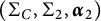



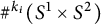


Proposition 4.3 The realization map
$\mathcal R$
 is well defined in the sense that any two pseudo-trisections constructed by the definition of
$\mathcal R$
 are indeed diffeomorphic.
Proof Suppose X and
$X'$
 are pseudo-trisected 4-manifolds constructed from a given pseudo-trisection diagram by
$\mathcal R$
 . Let
$X_i$
 and
$X_i'$
 be the sectors, W and
$W'$
 the 2-skeleta, and Z and
$Z'$
 be the 3-skeleta of X and
$X'$
 respectively. Notice that the 2-skeleta are exactly the union of the surfaces in the pseudo-trisection diagram, so we start with the identity map
$W \to W'$
 . Next, we extend this to a map
$Z \to Z'$
 by (the proof of) Proposition 2.13. This map restricts to diffeomorphisms
$\partial X_i \to \partial X_i'$
 as trisected 3-manifolds. Finally, we apply a theorem of Laudenbach and Poénaru [Reference Laudenbach and Poénaru15] which states that diffeomorphisms of
$\#k(S^1\times S^2)$
 extend to diffeomorphisms of
$\natural ^k(S^1\times B^3)$
 . Namely, the diffeomorphisms
$\partial X_i \to \partial X_i'$
 above each extend to maps
$X_i \to X^{\prime }_i$
 . These three extensions glue along Z to give a diffeomorphism
$X \to X'$
 .
Example 4.4 Figure 13 is an example of a pseudo-trisection diagram, namely of
$(S^2\times D^2) \natural (S^2\times D^2)$
 . Restricting the diagram to
$(\Sigma _1, \Sigma _2, \Sigma _3, \delta _1, \delta _2, \delta _3)$
 produces exactly the triple Heegaard diagram of
$(S^1\times S^2)\# (S^1\times S^2)$
 shown in Figure 8. On the other hand, the other triple Heegaard diagrams such as
$(\Sigma _C, \Sigma _1, \Sigma _2, \alpha _1, \delta _1, \alpha _2)$
 each describe
$S^1\times S^2$
 , so this is a valid pseudo-trisection diagram. One can show that the diagram really does encode
$(S^2\times D^2)\natural (S^2\times D^2)$
 by applying the realization map.
Example 4.5 Figure 14 depicts several of the simplest pseudo-trisection diagrams, by using the same choice of
$\Sigma _C, \Sigma _2$
 , and
$\Sigma _3$
 , but switching out
$\Sigma _1$
 and the associated curves.

In fact, these three diagrams are precisely the diagrams giving rise to the pseudo-trisections in Examples 3.12, 3.13, and 3.14.
Three pseudo-trisection diagrams (arising from three different choices of
$\Sigma _1$
 ).

Figure 14: Long description
The diagram is organized into two horizontal rows.
Top Row:
Three identical hemispherical surfaces are shown.
- The first on the left is labeled Sigma sub C.
- The middle is labeled Sigma sub 2.
- The right is labeled Sigma sub 3.
Bottom Row:
- On the far left is a single hemisphere labeled Sigma sub 1.
- In the center is a torus-like surface labeled Sigma prime sub 1. It features three vertical loops around its body. From left to right, these are a light blue loop labeled alpha sub 1, an orange dotted loop labeled delta sub 1, and a green loop labeled delta sub 3.
- On the far right is a similar torus-like surface labeled Sigma double prime sub 1. It contains the same orange dotted loop delta sub 1 and green loop delta sub 3. Additionally, it features a large light blue horizontal loop encircling the central hole, labeled alpha super asterisk sub 1.
Lemma 4.6 Fix a pseudo-trisection
$\mathcal T$
 of X. Any two pseudo-trisection diagrams
$\mathcal D$
 and
$\mathcal D'$
 with realization
$\mathcal T$
 are diffeomorphic after a sequence of handleslides and isotopies. (That is, there are diffeomorphisms
$\varphi _\circ : \Sigma _\circ \to \Sigma _\circ '$
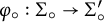 rel boundary preserving the arcs on the surfaces.)
Proof This essentially follows from the proof of Lemma 2.21. For each sector
$Y_i$
 or
$H_i$
 of the trisection, the corresponding meridian system (considered up to isotopy) [Reference Johannson11] is unique up to handleslides. A pseudo-trisection diagram is a collection of six overlapping meridian systems.
Note that handleslides and isotopies of pseudo-trisections are identical to those of triple Heegaard diagrams, described in Example 2.20.
Next we give diagrammatic descriptions of boundary stabilization, Heegaard stabilization, and internal stabilization. At the diagrammatic level, we find that Heegaard stabilization and internal stabilization fit into the same framework, which we call torus stabilization.
Definition 4.7 Given a pseudo-trisection diagram, a torus stabilization is a new pseudo-trisection diagram obtained by increasing the genus of one of the
$\Sigma _i$
 or
$\Sigma _C$
 by 1, and correspondingly adding three curves as shown in Figure 15. There are two types, as follows:
-
• Type I. Let $T^2$
be a torus with three curves, namely two meridians
$\mu _1, \mu _2$
and a longitude
$\gamma $
. For a fixed
$j \in \{1,2,3\}$
, a type I torus stabilization of
$(\Sigma _C, \Sigma _i, \boldsymbol \alpha _i, \boldsymbol \delta _{i})$
is the diagram obtained by replacing
$\Sigma _j$
with
$\Sigma _j \# T^2$
,
$\boldsymbol \alpha _j$
with
$\boldsymbol \alpha _j \cup \{\mu _1\}$
,
$\boldsymbol \delta _{j-1}$
with
$\boldsymbol \delta _{j-1}\cup \{\mu _2\}$
, and
$\boldsymbol \delta _j$
with
$\boldsymbol \delta _j \cup \{\gamma \}$
. -
• Type II. Let $(T^2, \mu _1, \mu _2, \gamma )$
be as above. For a fixed
$j \in \{1, 2, 3\}$
, a type II torus stabilization of
$(\Sigma _C, \Sigma _i, \boldsymbol \alpha _i, \boldsymbol \delta _{i})$
is the diagram obtained by replacing
$\Sigma _C$
with
$\Sigma _C \# T^2$
,
$\boldsymbol \alpha _j$
with
$\boldsymbol \alpha _j \cup \{\gamma \}$
,
$\boldsymbol \alpha _{j+1}$
with
$\boldsymbol \alpha _{j+1}\cup \{\mu _1\}$
, and
$\boldsymbol \alpha _{j-1}$
with
$\boldsymbol \alpha _{j-1} \cup \{\mu _2\}$
.





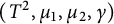




An example of a torus stabilization (which is type II with the given labels). See Definition 4.7.

Figure 15: Long description
The diagram consists of two panels showing the evolution of a topological surface.
Left Panel: A single-holed torus surface labeled below as open parenthesis Sigma sub C comma alpha sub i intersection Sigma sub C close parenthesis. Several colored curves wrap around the hole. From top to bottom, there is a blue curve, a pink curve, and an orange curve. These curves are solid on the visible front of the surface and dotted where they pass behind or through the surface. A vertical dotted black circle also wraps around the body of the torus.
Right Panel: The surface has been extended to the right to include a second hole, representing a connected sum. It is labeled below as open parenthesis Sigma sub C comma alpha sub i intersection Sigma sub C close parenthesis hash open parenthesis T super 2 comma gamma comma mu sub 1 comma mu sub 2 close parenthesis. The original curves from the left panel remain on the left side. On the new right-hand hole, three new circular curves are added: a blue circle on top, an orange circle on the bottom-left, and a pink circle on the bottom-right. These new curves intersect at a central point on the new torus handle.
One can check that torus stabilization is well defined by observing that the result of torus stabilization is a valid pseudo-trisection diagram, and moreover that it is a diagram of the same underlying 4-manifold.
Proposition 4.8 Torus stabilizations of pseudo-trisection diagrams correspond to Heegaard stabilizations and internal stabilizations of pseudo-trisections. More precisely, the following hold:
-
(1) Let $\mathcal D$
be a pseudo-trisection diagram with realization
$\mathcal T$
. Let
$\mathcal D'$
be a type I torus stabilization of
$\mathcal D$
. Then the realization of
$\mathcal D'$
is a Heegaard stabilization of
$\mathcal T$
. -
(2) Let $\mathcal T'$
be a Heegaard stabilization of
$\mathcal T$
. Then there is a pseudo-trisection diagram
$\mathcal D$
such that its realization is
$\mathcal T$
, and moreover a type I torus stabilization of
$\mathcal D$
has realization
$\mathcal T'$
. -
(3) Let $\mathcal D$
be a pseudo-trisection diagram with realization
$\mathcal T$
. Let
$\mathcal D'$
be a type II torus stabilization of
$\mathcal D$
. Then the realization of
$\mathcal D'$
is an internal stabilization of
$\mathcal T$
. -
(4) Let $\mathcal T'$
be an internal stabilization of
$\mathcal T$
. Then there is a pseudo-trisection diagram
$\mathcal D$
such that its realization is
$\mathcal T$
, and moreover a type II torus stabilization of
$\mathcal D$
has realization
$\mathcal T'$
.


Proof Item (1) is a direct consequence of the definition of realiation. Specifically, the connected sum of some
$\Sigma _j$
 with a torus results in the 3-dimensional 1-handlebodies
$H_j, Y_{j-1}$
 , and
$Y_j$
 each gaining a handle
$h_{H_j}, h_{Y_{j-1}}$
 , and
$h_{Y_j}$
 respectively. The curves added in the type I torus stabilization ensure that
$h_{H_j}$
 and
$h_{Y_{j-1}}$
 are parallel, while the other two pairs cancel. Gluing
$H_j \cup h_{H_j}, Y_{j-1} \cup h_{Y_{j-1}}$
 , and
$H_{j-1}$
 , we obtain a 3-manifold differing from
$\partial X_{j-1}$
 by a connected sum with
$S^1\times S^2$
 . This corresponds to the boundary of the handle attached in Heegaard stabilization.
To prove item (2) one can choose any pseudo-trisection diagram
$\mathcal D$
 of
$\mathcal T$
 . The Heegaard stabilization involves an arc
$\alpha $
 in some
$Y_j$
 with endpoints
$p, q$
 in
$\Sigma _j$
 , with neighborhood
$N(\alpha ) \subset Y_j$
 . Let
$\gamma _1$
 be the arc obtained by pushing
$\alpha $
 to the boundary of
$N(\alpha )$
 , and
$\gamma _2$
 the arc obtained by isotoping
$\alpha $
 onto
$\Sigma _j$
 and pushing the endpoints to agree with
$\gamma _1$
 . Let
$\gamma $
 be the closed curve
$\gamma _1 \cup \gamma _2$
 . Next, let
$\mu _1$
 and
$\mu _2$
 be meridians of
$N(\alpha )$
 . Create the diagram
$\mathcal D'$
 by a surgery replacing disks around p and q with an annulus corresponding to the boundary of
$N(\alpha )$
 , and add new curves
$\gamma , \mu _1, \mu _2$
 to the diagram as in the definition of type I torus stabilizations. After handleslides and isotopies of
$\gamma $
 , the resulting diagram is a type I torus stabilization of
$\mathcal D$
 which has realiation
$\mathcal T'$
 .
Items (3) and (4) are analogous to (1) and (2) and left to the reader.
Definition 4.9 Given a pseudo-trisection diagram, a band stabilization is a new pseudo-trisection diagram obtained by the following procedure:
-
(1) Identify a non-separating neatly embedded arc $\alpha $
in some
$\Sigma _i$
. Thicken the arc to a band in
$\Sigma _i$
. -
(2) New surfaces $\Sigma _i', \Sigma _{i+1}', \Sigma _{i+2}', \Sigma _C'$
are obtained by subtracting the band in
$\Sigma _i'$
, and attaching the band to the other three surfaces. -
(3) The preexisting curves on the surfaces are cut and pasted if they intersect the band, as shown by the change from $\delta _1$
to
$\delta _1'$
in Figure 16. Three new curves are added, one to each of
$\boldsymbol {\delta }_{i+1}, \boldsymbol {\alpha }_{i+1}$
, and
$\boldsymbol {\alpha }_{i+2}$
. Each curve consists of two arcs in the diagram, one in each corresponding surface. Each arc is a cocore of the attached band. See Figure 16 for a depiction of the case when
$i = 1$
.Figure 16:An example of a band stabilisation. See Definition 4.9.
Figure 16: Long description
The diagram consists of eight panels showing topological transformations.
Top row from left to right:
- Sigma sub 1: Two vertical lines containing a horizontal black curve alpha and an orange curve delta sub 1 that crosses alpha.
- Sigma sub 2: Two vertical lines with a small orange segment delta sub 1 attached to the right line.
- Sigma sub 3: Two vertical lines with no internal curves.
- Sigma sub C: Two vertical lines with no internal curves.
Bottom row from left to right:
- Sigma prime sub 1: The surface is split horizontally. An orange curve delta prime sub 1 is divided between the top and bottom sections.
- Sigma prime sub 2: A horizontal band connects the two surface sections. It contains a yellow vertical line alpha sub 2, a blue vertical line delta sub 2, and an orange diagonal line delta prime sub 1.
- Sigma prime sub 3: The horizontal band contains a blue vertical line delta sub 2 and a pink vertical line alpha sub 3.
- Sigma prime sub C: The horizontal band contains a yellow vertical line alpha sub 2 and a pink vertical line alpha sub 3.
Shaded grey regions indicate the interior of the surfaces behind the vertical boundary lines.





One can check that band stabilization is well defined by observing that the result is a pseudo-trisection diagram, and moreover that it is a diagram of the same underlying 4-manifold.
Proposition 4.10 Band stabilizations of pseudo-trisection diagrams correspond to boundary stabilizations of pseudo-trisections. More precisely, the following hold:
-
(1) Let $\mathcal D$
be a pseudo-trisection diagram with realization
$\mathcal T$
. Let
$\mathcal D'$
be a band stabilization of
$\mathcal D$
. Then the realization of
$\mathcal D'$
is a boundary stabilization of
$\mathcal T$
. -
(2) Let $\mathcal T'$
be a boundary stabilization of
$\mathcal T$
. Then there is a pseudo-trisection diagram
$\mathcal D$
such that its realization is
$\mathcal T$
, and moreover a band stabilization of
$\mathcal D$
has realization
$\mathcal T'$
.


Proof The proof is similar to the proof of Proposition 4.8. The equivalence is established by viewing the surfaces of the diagram as the 2-skeleton of the pseudo-trisection, and equating the arc
$\alpha $
 in the definition of band stabilization with the arc used in the definition of boundary stabilization.
Theorem 1.3 The realization map

induces a bijection

Proof This proof is analogous to that of Proposition 2.22. By Lemma 4.6, any two pseudo-trisection diagrams of a fixed pseudo-trisection are diffeomorphic after a sequence of handleslides and isotopies. By Theorem 1.2, any two pseudo-trisections of a given 4-manifold are equivalent up to boundary, Heegaard, and internal stabilization. By Propositions 4.10 and 4.8, band and torus stabilizations correspond to boundary, Heegaard, and internal stabilizations.
4.2 Boundary stabilization shift and relative existence
Boundary stabilization of pseudo-trisections is an extension of stabilization of 3-manifold trisections to the entire 4-manifold. In this subsection, we show that there is a reverse operation—destabilization of the boundary extends to the 4-manifold as well. We use this operation to establish that any trisection of the boundary 3-manifold of X extends to a pseudo-trisection of X. This mirrors the existence result for relative trisections [Reference Gay and Kirby7].
Definition 4.11 Boundary stabilization shift is an operation on pseudo-trisections with stabilized boundary defined diagrammatically in Figure 17 which can be thought of as exchanging a stabilization of the boundary for an internal stabilization. The details are as follows:
-
(1) Let X be equipped with a pseudo-trisection $\mathcal T$
such that
$\mathcal T|_{\partial X}$
is a stabilisation of a trisection
$\tau '$
of
$\partial X$
. -
(2) Let $(\Sigma _C, \Sigma _i, \boldsymbol {\alpha }_i, \boldsymbol {\delta }_i)$
be a pseudo-trisection diagram of
$\mathcal T$
realizing the stabilisation of the boundary. (This is the top row of Figure 17.) Locally, each of
$\Sigma _1, \Sigma _2$
, and
$\Sigma _3$
are as depicted by shading, but nothing can be said about how
$\Sigma _C$
meets its boundary. -
(3) The boundary stabilisation shift of $\mathcal T$
is the pseudo-trisection given by the diagram in the bottom row of Figure 17. This is obtained by band surgery on each of
$\Sigma _i$
and
$\Sigma _C$
: a band is glued to obtain each of
$\Sigma _1'$
and
$\Sigma _C'$
, with a corresponding meridian in
$\boldsymbol {\alpha }_1$
, and bands are deleted to obtain
$\Sigma _2'$
and
$\Sigma _3'$
.





A diagrammatic definition of boundary stabilisation shift, see Definition 4.11.

Figure 17: Long description
The diagram consists of two rows of four panels each.
Top Row:
- Panel 1: Labeled Sigma sub 1. Shows two vertical parallel lines with a horizontal gap between them.
- Panel 2: Labeled Sigma sub 2. Similar to Sigma sub 1 but with a light gray shaded region between the lines and a blue vertical segment labeled gamma in delta sub 2 connecting the upper and lower boundaries.
- Panel 3: Labeled Sigma sub 3. Identical to Sigma sub 2, showing the same gamma in delta sub 2 segment.
- Panel 4: Labeled Sigma sub C. Shows the two vertical lines with the horizontal gap, similar to Sigma sub 1 but with light gray shading extending from the boundaries.
Bottom Row:
- Panel 5: Labeled Sigma sub 1 prime. Shows a narrow channel formed by inward-protruding rectangular boundaries. A blue horizontal segment is labeled mu in alpha sub 1.
- Panel 6: Labeled Sigma sub 2 prime. Shows the same narrow channel geometry without the blue segment or internal labels.
- Panel 7: Labeled Sigma sub 3 prime. Identical geometry to Sigma sub 2 prime.
- Panel 8: Labeled Sigma sub C prime. Shows the narrow channel geometry with the blue horizontal segment labeled mu in alpha sub 1 and light gray shading concentrated around the central constriction.
Lemma 4.12 Boundary stabilisation shift is well defined.
Proof Referring back to Definition 4.1, being well defined requires that each
$\boldsymbol {\delta }_i$
 and
$\boldsymbol {\alpha }_i$
 must be a cut system of its corresponding surface, and that each of the triple Heegaard diagrams induced on the three triples
$(\Sigma _C', \Sigma _i', \Sigma _{i+1}')$
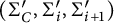 are specifically diagrams of connected sums of
$S^1\times S^2$
 .
For the first condition, observe that the only surface-pairs whose unions have changed in the operation are
$\Sigma _2' \cup \Sigma _3'$
 and
$\Sigma _1' \cup \Sigma _C'$
 . In the former, the genus is decreased by a surgery along a neighborhood of
$\gamma $
 , so
$\boldsymbol {\delta }_2 - \{\gamma \}$
 is a cut system of
$\Sigma _2' \cup \Sigma _3'$
 . In the latter, the genus is increased and
$\mu $
 is the corresponding meridian, so
$\boldsymbol {\alpha }_1 \cup \{\mu \}$
 is a cut system.
For the second condition, we observe that
$(\Sigma _C', \Sigma _1', \Sigma _2', \boldsymbol {\alpha }_1 \cup \{\mu \}, \boldsymbol {\delta }_1, \boldsymbol {\alpha }_2)$
 is a stabilisation of
$(\Sigma _C, \Sigma _1, \Sigma _2, \boldsymbol {\alpha }_1, \boldsymbol {\delta }_1, \boldsymbol {\alpha }_2)$
 . The latter is necessarily a diagram of
$\#^{k_1}(S^1\times S^2)$
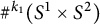 because our operation is on a valid pseudo-trisection diagram. Consequently,
$(\Sigma _C', \Sigma _1', \Sigma _2', \boldsymbol {\alpha }_1\cup \{\mu \}, \boldsymbol {\delta }_1, \boldsymbol {\alpha }_2)$
 is a diagram of
$\#^{k_1}(S^1\times S^2)$
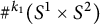 . Similarly,
$(\Sigma _C', \Sigma _3', \Sigma _1', \boldsymbol {\alpha }_3, \boldsymbol {\delta }_3, \boldsymbol {\alpha }_1 \cup \{\mu \})$
 is a diagram of
$\#^{k_3}(S^1\times S^2)$
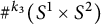 . The remaining check is that
$(\Sigma _C', \Sigma _2', \Sigma _3', \boldsymbol {\alpha }_2, \boldsymbol {\delta }_2 \cup \{\gamma \}, \boldsymbol {\alpha }_3)$
 is locally a destabilisation of
$(\Sigma _C, \Sigma _2, \Sigma _3, \boldsymbol {\alpha }_2, \boldsymbol {\delta }_2, \boldsymbol {\alpha }_3)$
 , so it is a diagram of
$\#^{k_2}(S^1\times S^2)$
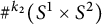 .
Proposition 4.13 Boundary stabilisation shift of
$\mathcal T$
 to
$\mathcal T'$
 satisfies the following properties:
-
(1) $\mathcal T|_{\partial X}$
is a stabilisation of
$\mathcal T'|_{\partial X}$
(in the sense of 3-manifold trisections). -
(2) Complexity of the pseudo-trisection is invariant under boundary stabilisation shift, while complexity of the boundary decreases by 1.
-
(3) Suppose $\mathcal T$
is a boundary stabilisation of a pseudo-trisection
$\mathcal T^*$
. Then
$\mathcal T'$
is an internal stabilisation of
$\mathcal T^*$
.


Proof Item (1). This is an immediate consequence of the definition, by restricting the diagram to
$(\Sigma _i', \boldsymbol {\delta }_i')$
 and observing that it stabilizes to
$(\Sigma _i, \boldsymbol {\delta }_i).$

Item (2). The complexity of the pseudo-trisection is unchanged since each
$k_i$
 is unchanged (as was observed in the proof of Lemma 4.12.) The complexity of the boundary decreases by 1, by Proposition 2.26.
Item (3). This is proved diagrammatically, in Figure 18. The top row shows local regions of a pseudo-trisection diagram of
$\mathcal T^*$
 , and
$\alpha $
 denotes the curve along which the boundary stabilisation occurs. Applying a boundary stabilisation along
$\alpha $
 followed by a boundary stabilisation shift, the resulting pseudo-trisection diagram is shown in the second row. Applying diffeomorphisms to the
$\Sigma _i'$
 and
$\Sigma _C'$
 , and isotoping the curves, the bottom row is obtained. Applying handleslides and isotopies to
$\mu $
 , and a diffeomorphism rel boundary to
$\Sigma _C'$
 , the diagram of the bottom row can be expressed as a type II torus stabilisation of the initial diagram. The result now follows from Proposition 4.8.
Proof of Proposition 4.13, item (3).

Figure 18: Long description
The diagram consists of three rows and four columns of panels.
Top Row:
- Panel 1: Sigma super star sub 1 shows two vertical lines with a shaded region between them and a horizontal curve alpha.
- Panel 2: Sigma super star sub 2 shows two vertical lines with shading on the outer sides.
- Panel 3: Sigma super star sub 3 is identical to the second panel.
- Panel 4: Sigma super star sub C is identical to the second and third panels.
Middle Row:
- Panel 1: Sigma prime sub 1 shows a surface with a narrow neck containing a blue horizontal line mu and a vertical arc.
- Panel 2: Sigma prime sub 2 shows the neck split into two separate rounded ends labeled gamma sub 2.
- Panel 3: Sigma prime sub 3 shows a similar split with labels gamma sub 3.
- Panel 4: Sigma prime sub C shows a combined view with labels gamma sub 2, gamma sub 3, and mu.
Bottom Row:
- Panel 1: Sigma prime sub 1 shows two vertical lines with a straight blue horizontal line mu.
- Panel 2: Sigma prime sub 2 shows two vertical lines with outer shading.
- Panel 3: Sigma prime sub 3 is identical to the second panel.
- Panel 4: Sigma prime sub C shows a three-dimensional cylinder extending from the left vertical line toward the right. A blue line mu runs through the cylinder. On the right side, three concentric colored loops (yellow, orange, and pink) are labeled gamma sub 2 and gamma sub 3.
Theorem 1.1 Let X be a compact oriented 4-manifold with non-empty connected boundary Y. Let
$\tau $
 be a trisection of Y. Then there is a pseudo-trisection
$\mathcal T_1$
 of X such that
$\mathcal T_1 |_{Y} = \tau $
 .
Proof Case 1:
$\tau $
 is the trivial trisection of
$Y = S^3$
 . Fill the boundary Y with a 4-ball
$B^4$
 to obtain a closed manifold
$X\cup B^4$
 . There is a trisection of
$X\cup B^4$
 by the usual existence result in the closed setting [Reference Gay and Kirby7]. Choose any point in the central surface of the trisection, and there is a trivially trisected neighborhood N of the point. Now X is diffeomorphic to
$(X \cup B^4) - N$
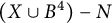 , and the latter is equipped with a pseudo-trisection with boundary
$\tau $
 .
Case 2: Y is equipped with any trisection
$\tau $
 other than the trivial trisection of
$S^3$
 . (Y may or may not be
$S^3$
 .) Equip X with a pseudo-trisection
$\mathcal T$
 by Corollary 3.20. By Proposition 2.10, there is a trisection
$\tau '$
 of Y such that there is a sequence of stabilisations and Heegaard stabilisations from
$\mathcal T|_Y$
 to
$\tau '$
 , and a sequence of stabilisations from
$\tau $
 to
$\tau '$
 . At the 4-dimensional level, there is an induced sequence of boundary stabilisations and Heegaard stabilisations from
$\mathcal T$
 to some pseudo-trisection
$\mathcal T'$
 with
$\mathcal T'|_Y = \tau '$
 . Further, there is a sequence of boundary stabilisation shifts from
$\mathcal T'$
 to a pseudo-trisection
$\mathcal T_1$
 with
$\mathcal T_1|_Y = \tau $
 .
4.3 Orientations of pseudo-trisections
In this subsection, we outline a convention for how a pseudo-trisection diagram determines an orientation of the corresponding 4-manifold. In general, this requires one additional label to be added to the pseudo-trisection diagram.
-
(1) If the binding of the pseudo-trisection consists of one component and is depicted as a circle in the given pseudo-trisection diagram, it is oriented counterclockwise. Otherwise, one component of the binding must be labeled with an orientation.
-
(2) The orientation of the boundary component extends to an orientation of the surfaces $\Sigma _\circ , \circ \in \{C, 1, 2, 3\}$
by the outward-normal-first convention. (This further induces orientations on any remaining components of the binding.) -
(3) An oriented normal vector to each $\Sigma _\circ $
is determined by the right hand rule. Pieces of the 3-skeleton are oriented as follows:-
(a) The boundary $\partial Y_i$
of
$Y_i$
is oriented as
$(-\Sigma _i) \cup \Sigma _{i+1}$
. Now
$Y_i$
is oriented by the outward-normal-first convention. -
(b) The boundary $\partial H_i$
of
$H_i$
is oriented as
$(-\Sigma _C) \cup \Sigma _i$
. Now
$H_i$
is oriented by the outward-normal-first convention.
-
-
(4) Next, the boundaries $\partial X_i$
of the sectors are oriented as
$Y_i \cup H_i \cup (-H_{i+1})$
. The sectors
$X_i$
are oriented by the outward-normal-first convention. -
(5) The 4-manifold X is oriented as $X_1 \cup X_2 \cup X_3$
. The boundary
$\partial X = Y$
is oriented as
$Y_1 \cup Y_2 \cup Y_3$
, and this orientation agrees with the induced boundary orientation from X.



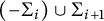







5 Pseudo-bridge trisections
In this section, we extend from considering 4-manifolds to considering pairs
$(X, \mathcal K)$
 where
$\mathcal K$
 is an embedded surface. In the case where X and
$\mathcal K$
 are closed, these pairs are understood via bridge trisections as in [Reference Meier and Zupan19]. In the relative case (i.e., when X is compact with boundary
$\partial X$
 , and
$\mathcal K \subset X$
 is a neatly embedded surface with boundary
$L \subset \partial X$
 ), there is a notion of relative bridge trisections introduced in general in [Reference Meier17]. We summarize relative bridge trisections before introducing an analog of bridge position for pseudo-trisections. We also introduce pseudo-bridge trisection diagrams and describe how some properties of the encoded surface can be read off the diagrams. Recall the conventions for pairs
$(X, \mathcal K)$
 described in Section 1—the introduction.
5.1 Relative bridge trisections
The general theory of relative bridge trisections, due to Meier [Reference Meier17], is reviewed here.
In the same way that relative trisections are defined to be determined by the spine (equivalently, a diagram on the central surface), relative bridge trisections are defined so that the embedded surface is encoded by a diagram on the central surface (without, for example, having to describe the boundary link of the surface). This is achieved through additional Morse-theoretic structure.
Suppose X is equipped with a relative trisection. Let
$N(B)$
 be a tubular neighborhood of the binding of the relative trisection. Each
$H_i' = (X_i \cap X_{i+1}) - N(B)$
 has the structure of a compression body between two surfaces with boundary, namely
$\Sigma _C' = \Sigma _C - N(B)$
 and
$\Sigma _{i+1}' = \Sigma _{i+1} - N(B)$
 . By virtue of being a compression body, there is a standard self-indexing Morse function
$\Phi _i$
 which vanishes exactly on
$\Sigma _C'$
 and is maximised exactly on
$\Sigma _{i+1}'$
 . Let
$\tau _i$
 be a tangle in
$H_i$
 . It can be assumed that
$\tau _i$
 lies in
$H_i'$
 because
$\tau _i$
 avoids B by the transversality theorem. After an isotopy of
$\tau _i$
 ,
$\Phi _i$
 restricted to
$\tau _i$
 is Morse. An arc in
$\tau _i$
 is vertical if it has no local extrema, and is flat if it has a unique local extremum, which is a maximum.
Definition 5.1 Let
$\tau _i$
 be a tangle in
$H_i$
 . This is a
$(b,v)$
 -tangle if it is isotopic rel boundary to a tangle consisting exactly of b flat arcs and v vertical arcs. The v vertical arcs may end in separate components of
$\partial X$
 , in which case the components are ordered and we have a
$(b,\boldsymbol v)$
 -tangle where
$\boldsymbol v$
 is an ordered partition of v.
In relative trisections the compressionbodies
$H_i$
 are also handlebodies; the notion of triviality above ensures that all arcs can be simultaneously isotoped to lie in the boundary.
Definition 5.2 Let
$\mathcal {D}_i$
 be a disk-tangle in
$X_i$
 . This is a trivial tangle if it can be isotoped rel boundary to lie in
$\partial X_i$
 . In this case the boundary is an unlink in
$H_i \cup H_{i-1}$
 , and we say
$\partial \mathcal {D}_i$
 is in
$(b,\boldsymbol v)$
 -bridge position if the tangles in
$H_i$
 and
$H_{i-1}$
 are both
$(b,\boldsymbol v)$
 -tangles. Given that the boundary link of
$\partial X_i$
 is in
$(b,\boldsymbol v)$
 -bridge position, we say that
$\mathcal {D}_i$
 is a
$(c,\boldsymbol v)$
 -disk-tangle, where
$c+v$
 is the number of components of
$\mathcal {D}_i$
 .
Definition 5.3 Let X be a compact 4-manifold with boundary, and
$\mathcal K$
 a neatly embedded surface in X. Let
$b,c, v$
 be non-negative integers,
$\boldsymbol v$
 an ordered partition of v into non-negative integers, and
$\boldsymbol c$
 an ordered partition of c into three non-negative integers. The surface
$\mathcal K$
 is in
$(b,\boldsymbol c; \boldsymbol v)$
 -bridge trisected position in a relative trisection of X if
-
(1) each $\mathcal D_i = X_i \cap \mathcal K$
is a trivial
$(c_i; \boldsymbol v)$
-disk-tangle in
$X_i$
, and -
(2) each $\tau _i = H_i \cap \mathcal K$
is a
$(b;\boldsymbol v)$
-tangle in
$H_i$
.



Remark 5.4 The above definition requires a lot of structure, keeping track of
$(b,\boldsymbol c;\boldsymbol v)$
 . This is essentially so that the
$\tau _i$
 are enough to encode the surface. In the case of pseudo-bridge trisections, we’ll introduce a more general notion of bridge position for which the analogs of
$\tau _i$
 aren’t enough to encode the surface, but projections of tangles onto each surface in the pseudo-trisection diagram are enough. The overarching idea is that we’re generalizing the notion of bridge position in such a way as to obtain conceptually simpler diagrams and lower diagram complexity for a fixed surface (e.g., lower bridge index), but in exchange for diagrams with more pieces.
5.2 Pseudo-bridge trisections
Next we introduce pseudo-bridge trisections, the analog of relative bridge trisections in the setting of pseudo-trisections. We also introduce pseudo-shadow diagrams, which are analogous to shadow diagrams of relative bridge trisections. We show how a pseudo-shadow diagram uniquely encodes a pseudo-bridge trisection up to isotopy. We will immediately see that any pair
$(X,\mathcal K)$
 admits a pseudo-bridge trisection by application of the existence of relative bridge trisections.
Definition 5.5 Let X be a pseudo-trisected 4-manifold, and let
$\mathcal K \subset X$
 be a neatly embedded surface. The surface
$\mathcal K$
 is in pseudo-bridge position if
-
(1) each $\mathcal D_i = X_i \cap \mathcal K$
is a trivial disk-tangle in
$X_i$
, and -
(2) each $\tau _i = H_i \cap \mathcal K$
and
$L_i = Y_i \cap \mathcal K$
is a trivial tangle in
$H_i$
and
$Y_i$
respectively.



Note that here a tangle is trivial if it can be isotoped rel boundary to lie in the boundary of the ambient space. A bridge point of the pseudo-bridge trisection is any point lying on the intersection between
$\mathcal K$
 and the 2-skeleton of the pseudo-trisection. The data of a pseudo-trisection together with a surface in pseudo-bridge position is termed a pseudo-bridge trisection.
Example 5.6 The standard disk
$D^2$
 in
$B^4$
 admits a pseudo-bridge trisection which is also a relative bridge trisection. See Figure 19 (A).
-
(1) Let $B^4$
be the standard unit ball in
$\mathbb {R}^4$
expressed in
$\{r, \theta ,z,w\}$
-coordinates. -
(2) The trivial pseudo-trisection of $B^4$
3.12 (which is also a relative trisection) is given by decomposing into sectors with
$0 \leq \theta \leq 2\pi /3$
,
$2\pi /3 \leq \theta \leq 4\pi /3$
, and
$4\pi /3 \leq \theta \leq 2\pi $
. -
(3) A standard disk embedding is given by $(z,w) = (0,0)$
. This disk intersects the aforementioned pseudo-trisection in bridge position.


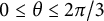



One can show that this is a relative bridge trisection of the standard disk.
Schematics of two distinct pseudo-bridge trisections of a standard disk in
$B^4$
 .

Figure 19: Long description
The figure contains two panels, A and B, each showing a sphere divided by three intersecting planes meeting at a central vertical axis.
Panel A, titled A standard disk in relative bridge position, shows a horizontal gray disk centered within the sphere. The disk is divided into three sectors by three radial line segments labeled tau sub 1, tau sub 2, and tau sub 3, which meet at the center. The outer boundary of the disk is composed of three arcs labeled L sub 1, L sub 2, and L sub 3. L sub 1 is orange, L sub 2 is blue, and L sub 3 is green. Each arc lies on one of the three dividing planes of the sphere.
Panel B, titled A standard disk in pseudo-bridge position, shows a similar sphere but with a disk oriented differently. The disk is shaded gray and appears tilted. It is bounded by arcs L sub 1 and L sub 3. A light blue shaded region occupies one of the vertical trisection planes. A radial line segment labeled tau sub 1 extends from the central axis to the boundary arc L sub 1. The intersection of the disk with the trisection planes creates a distinct geometric configuration compared to panel A.
Example 5.7 The standard disk in
$B^4$
 also admits a simpler pseudo-bridge trisection with less symmetry, which in particular is not a relative bridge trisection. See Figure 19 (B).
-
(1) Let $B^4$
be parametrized and trisected as in Example 5.6. -
(2) Consider the cartesian parametrization of $\mathbb {R}^4$
, that is,
$(x,y, z, w) = (r\cos \theta , r\sin \theta , z, w)$
. The plane
$(x,w) = (1/2, 0)$
intersects
$B^4$
along a standard disk as a pseudo-bridge trisection.





This pseudo-trisection fails to be a relative trisection for Morse theoretic reasons: although
$\tau _1$
 is a trivial tangle, it has a local minimum and cannot be isopted to be flat or vertical.
Remark 5.8 Any
$(X,\mathcal K)$
 admits a pseudo-bridge trisection. First, there is a relative trisection
$\mathcal T$
 of X with non-empty binding by the existence result of Gay and Kirby [Reference Gay and Kirby7]. Such a relative trisection is necessarily a pseudo-trisection by Proposition 3.18. On the other hand, by the existence result of Meier [Reference Meier17],
$(X,\mathcal K)$
 admits a relative bridge trisection whose underlying relative trisection is
$\mathcal {T}$
 . This relative bridge trisection is necessarily a pseudo-bridge trisection.
5.3 Pseudo-shadow diagrams
Shadow diagrams [Reference Meier17] are a diagrammatic theory of relative bridge trisections compatible with relative trisection diagrams. Here we introduce pseudo-shadow diagrams, a diagrammatic theory of pseudo-bridge trisections compatible with pseudo-trisection diagrams. In particular, any pair
$(X,\mathcal K)$
 admits a description by a pseudo-shadow diagram.
Definition 5.9 Let
$\mathcal K, \mathcal K' \subset X$
 . The surfaces
$\mathcal K$
 and
$\mathcal K'$
 are neatly isotopic if they are homotopic through neat embeddings.
Proposition 5.10 A pseudo-bridge trisected surface
$\mathcal K \subset X$
 is determined up to neat isotopy by the 3-skeleton of the pseudo-bridge trisection, that is, by the data of all the tangles
$(H_i, \tau _i)$
 ,
$(Y_i, L_i)$
 , and how they intersect.
Proof The data of the 3-skeleton describes how the triples
$((H_i, \tau _i),(H_{i+1}, \tau _{i+1}),(Y_i, L_i))$
 glue together to produce links in the boundaries of the sectors
$X_i$
 . These links are necessarily unlinks, which bound unique trivial disk-tangles in the sectors up to neat isotopy. Compare with [Reference Meier and Zupan19, Lemma 2.3 and Corollary 2.4].
Consequently, we can define an analog of shadow diagrams as follows.
Definition 5.11 A pseudo-shadow diagram consists of the data
$(\mathcal D, \tau _1, \tau _2, \tau _3, L_1,L_2,L_3)$
 where
-
(1) $\mathcal {D} = (\Sigma _C, \Sigma _i, \boldsymbol \alpha _i, \boldsymbol \delta _i)$
is a pseudo-trisection diagram. -
(2) For $i \in \{1,2,3\}$
,
$\tau _i$
is a collection of generically embedded arcs in
$\Sigma _i \cup \Sigma _{C}$
, all with distinct endpoints. If any two arcs in a given
$\tau _i$
cross, the crossing order is indicated. The arcs intersect
$B = \partial \Sigma _i = \partial \Sigma _C$
transversely. -
(3) Similarly, each $L_i$
is a collection of generically embedded arcs in
$\Sigma _i \cup \Sigma _{i+1}$
with distinct endpoints. If any two cross, the crossing order is indicated. Any intersections with B are transverse. -
(4) For any i, $\tau _i, L_i$
, and
$L_{i-1}$
may intersect
$\Sigma _i$
. Each of these families of arcs are pairwise transverse in
$\Sigma _i$
. -
(5) There is a collection of points $\mathcal B_i \subset \Sigma _i$
which consists precisely of the endpoints of
$\tau _i, L_i$
, and
$L_{i-1}$
that lie in
$\Sigma _i$
. (Consequently, each point in
$\mathcal B_i$
has degree 3 in a pseudo-shadow diagram.) -
(6) The above two points also hold verbatim for $(\Sigma _C, \tau _1, \tau _2, \tau _3)$
instead of
$(\Sigma _i, \tau _i, L_i, L_{i-1})$
.The set of endpoints of arcs in
$\tau _i$
lying in
$\Sigma _C$
is denoted
$\mathcal B_C$
. -
(7) The unions $\tau _i \cup \tau _{i+1} \cup L_i$
form unlinks in each of the 3-dimensional manifolds encoded by the corresponding triple Heegaard diagram in the underlying pseudo-trisection diagram.











For notational brevity, we frequently write
$(\mathcal D, \tau _i, L_i)$
 instead of
$(\mathcal D, \tau _1, \tau _2, \tau _3, L_1,L_2,L_3)$
 .
Definition 5.12 There is a realization map

extending the realization map of Definition 4.2 defined as follows:
-
(1) A pseudo-shadow diagram has an underlying pseudo-trisection diagram. First, this is mapped to a pseudo-trisection by the realization map of Definition 4.2.
-
(2) Each collection of arcs $\tau _i$
and
$L_i$
lies in the 2-skeleton of the above pseudo-trisection. Each collection is isotoped rel boundary to form a tangle in
$H_i$
and
$Y_i$
, respectively. -
(3) Each triple union $\tau _i \cup \tau _{i+1} \cup L_i$
forms an unlink in
$\partial X_i$
. This bounds a collection of disks in
$\partial X_i$
(uniquely up to isotopy rel boundary). -
(4) The above collections of disks are isotoped rel boundary to be neatly embedded in $X_i$
. The result is now a pseudo-bridge trisection.





Proposition 5.13 The realization map of Definition 5.12 is well defined.
Proof We must show that the map as defined truly sends a pseudo-shadow diagram to a pseudo-bridge trisection, and that any two pseudo-bridge trisections built from the same pseudo-shadow diagram by the map are neatly isotopic. (More precisely, after a diffeomorphism, the embedded surfaces differ by neat isotopy.)
Let
$(X, \mathcal K)$
 be the realization of a pseudo-shadow diagram
$\mathcal D$
 . Then each
$\mathcal K \cap X_i$
 is necessarily a trivial disk tangle, because it is obtained by isotoping a collection of disks rel boundary from
$\partial X_i$
 to
$X_i$
 . Similarly, each
$\mathcal K \cap H_i$
 and
$\mathcal K \cap Y_i$
 is necessarily a trivial tangle. It follows that
$(X, \mathcal K)$
 is a pseudo-bridge trisection.
Next, suppose
$(X, \mathcal K)$
 and
$(X',\mathcal K')$
 are realizations of the same pseudo-shadow diagram
$\mathcal D$
 . By Proposition 4.3, the underlying 4-manifolds X and
$X'$
 and their pseudo-trisections are diffeomorphic. Hereafter
$\mathcal K, \mathcal K'$
 are considered to both lie in X. The arcs
$\tau _i$
 and
$L_i$
 lift to the 2-skeleton of the pseudo-trisection of X, and are further isotoped into
$H_i$
 and
$Y_i$
 respectively to produce exactly the 3-skeleta of
$(X, \mathcal K)$
 and
$(X, \mathcal K')$
 . By Proposition 5.10, the 3-skeleta determine the surface in pseudo-bridge position up to neat isotopy.
Example 5.14 Figure 20 is a pseudo-shadow diagram. This can be verified by inspecting the definition of a pseudo-shadow diagram. The most interesting condition is item (7). The union
$\tau _1 \cup \tau _2 \cup L_1$
 consists of an unknot in
$B^3$
 , as shown in Figure 21.
A pseudo-shadow diagram of a disk in relative bridge position in
$B^4$
 .

The knot
$\tau _1\cup \tau _2 \cup L_1 \subset S^3$
 , see Example 5.14.

The underlying pseudo-trisection diagram of the aforementioned pseudo-shadow diagram is that of the trivial trisection (of
$B^4$
 ). The surface is built by applying the realization map. Explicitly, the arcs
$\tau _1, \tau _2$
 , and
$L_1$
 lift to an unknot in
$\partial X_1 = B^3$
 . Similarly,
$\tau _2, \tau _3, L_2$
 lift to an unknot in
$\partial X_2 = B^3$
 . The common intersection of these two unknots is
$\tau _2$
 . The two unknots next encode disks in
$X_1$
 and
$X_2$
 respectively, and the union of these disks is itself a disk in
$X_1 \cup X_2$
 with boundary
$\tau _1 \cup \tau _3 \cup L_1 \cup L_2$
 . Finally,
$\tau _1 \cup \tau _3 \cup L_3$
 lifts to an unknot in
$\partial X_3$
 , which bounds a disk in
$X_3$
 . Gluing in this final disk produces a disk in X exactly as in Figure 19 (A).


5.4 Resolving crossings in pseudo-shadow diagrams
When applying the realization map, arcs in the pseudo-shadow diagram are lifted from the 2-skeleton into the 3-skeleton. Crossings between arcs are resolved in different ways depending on the types of arcs, as well as whether or not the orientations of the underlying surface and 3-manifold are compatible. For example, in Section 4.3, we saw that
$\partial Y_i = (-\Sigma _i) \cup \Sigma _{i+1}$
 as an oriented union. Lifting a crossing from
$\Sigma _i$
 to
$Y_i$
 may reverse it, while lifting from
$\Sigma _{i+1}$
 to
$Y_i$
 may preserve it. The following list outlines how to resolve any crossing when realizing a pseudo-bridge diagram.
Remark 5.16 The actual choice or convention happens when we declare how an orientation of the binding (of a pseudo-trisection diagram) induces an orientation of the pseudo-trisected 4-manifold. This determines exactly how arcs in a pseudo-shadow diagram must lift to the 4-manifold. The rules being outlined below should be thought of as “what do crossings between arcs in a pseudo-shadow diagram actually represent, given the orientation conventions from Section 4.3?”.
-
(1) For each i, consider the oriented pairs $(\partial X_i, \Sigma _i), (\partial X_i, \Sigma _{i+1}), (\partial X_i, \Sigma _C)$
, and
$(Y, \Sigma _i)$
. Each of the twelve pairs is further equipped with a normal vector field on
$\Sigma _{\circ }, \circ \in \{i, i+1, C\}$
which extends the orientation of
$\Sigma _\circ $
to agree with the orientation of the ambient 3-manifold. -
(2) In a pseudo-shadow diagram, $L_{i-1}$
lies above
$L_{i}$
in the sense that any arcs of
$L_{i-1}$
intersecting arcs of
$L_{i}$
in
$\Sigma _{i}$
lift to a position above
$L_{i}$
with respect to the aforementioned normal vector field on
$(Y, \Sigma _{i})$
. Similarly,
$\tau _i$
lies above
$L_i$
;
$L_i$
lies above
$\tau _{i+1}$
; and
$\tau _{i+1}$
lies above
$\tau _i$
. (Note that specifying two tangles in the pseudo-shadow diagram determines a unique ambient pair
$(\partial X_i, \Sigma _i), \ldots , (Y, \Sigma _i)$
.) -
(3) Any self-crossings, that is, crossings of $L_i$
or
$\tau _i$
with themselves in
$\Sigma _\circ $
, necessarily have crossing order indicated in the diagram. We say crossing orders are preserved if the over-strand lies above the under-strand and reversed otherwise. We have:-
(a) Self-crossings of $L_{i}$
in
$(Y, \Sigma _{i+1})$
and
$(\partial X_{i}, \Sigma _{i+1})$
are preserved; self-crossings of
$L_i$
in
$(Y, \Sigma _i)$
and
$(\partial X_i, \Sigma _i)$
are reversed. -
(b) Self-crossings of $\tau _i$
in
$(\partial X_i, \Sigma _i)$
and
$(\partial X_{i-1}, \Sigma _C)$
are preserved; self-crossings of
$\tau _i$
in
$(\partial X_i, \Sigma _C)$
and
$\partial X_{i-1}, \Sigma _i)$
are reversed.
-








Example 5.17 Figure 23 is a valid pseudo-shadow diagram of a neatly embedded surface
$\mathcal K$
 in
$B^4$
 . The boundary link
$L_1 \cup L_2 \cup L_3 = \partial \mathcal K \subset S^3$
 is easily seen to arise from a knot diagram with three crossings. However, determining whether it is an unknot, a left-handed trefoil, or right-handed trefoil requires some care.
We observe that the self-crossings are:
$L_3$
 in
$\Sigma _1$
 ,
$L_1$
 in
$\Sigma _2$
 , and
$L_2$
 in
$\Sigma _3$
 . It follows that each of the three self-crossings are preserved. Since every crossing is a negative crossing, it follows that the boundary knot is a left-handed trefoil.
A pseudo-shadow diagram of a genus 1 surface in
$B^4$
 with boundary a trefoil knot. The boundary knot is given by
$L_1, L_2,$
 and
$L_3$
 .

Figure 23: Long description
The figure consists of four circular panels arranged horizontally.
* Panel 1 (Sigma sub C): Contains six line segments radiating from a central gap toward the perimeter. On the left, segments are labeled tau sub 2 (yellow), tau sub 3 (pink), and tau sub 1 (blue). On the right, three unlabeled segments mirror these colors.
* Panel 2 (Sigma sub 1): Features a green braided pair at the top labeled L sub 3. Below this, two orange parallel lines labeled L sub 1 descend to the bottom left. A single blue line labeled tau sub 1 extends to the right perimeter.
* Panel 3 (Sigma sub 2): Shows a yellow line tau sub 2 at the top. Below it, two orange lines labeled L sub 1 twist around each other on the left. A blue line labeled L sub 2 runs parallel to them on the right.
* Panel 4 (Sigma sub 3): Displays two vertical green lines at the top labeled L sub 3. A pink line labeled tau sub 3 extends to the left. Below, two blue lines labeled L sub 2 twist together and exit toward the bottom right.
5.5 Pseudo-shadow diagram examples and calculations
In this subsection, we provide several examples of pseudo-shadow diagrams, and show how to compute some invariants such as orientability (of the embedded surface), the intrinsic topology of the surface, and the homology class represented by the surface in the ambient 4-manifold.
Proposition 5.18 A surface realizing a pseudo-shadow diagram is orientable if and only if the graph
$\bigcup _i (L_i \cup \tau _i) \subset (\bigcup _i \Sigma _i) \cup \Sigma _C$
 can be consistently labeled such that every vertex is either a source or a sink. (In this context the vertices are the bridge points and the intersections of the
$L_i$
 and
$\tau _i$
 with the binding.)
Proof This follows directly from the orientation convention of Section 4.3.
Example 5.19 Figure 24 is a pseudo-shadow diagram of a Möbius strip in
$\mathbb {CP}^2 - B^4$
 . To see that the surface represented by the diagram is non-orientable, observe that the vertices
$b_1, b_2, b_3$
 lie in a 3-cycle
$\gamma $
 in the graph
$\bigcup _i (L_i \cup \tau _i)$
 , and therefore cannot be consistently labeled as sources or sinks. (For such a labeling to exist, any cycle must have even length.)
A pseudo-shadow diagram of a Möbius strip in pseudo-bridge position in
$\mathbb {CP}^2 - B^4$
 .

Figure 24: Long description
The diagram consists of two main sections.
On the left is a square fundamental domain labeled Sigma sub C at the bottom. The square has black boundary lines with arrows indicating identification. Inside the square, a large white circle is centered. Several dashed and solid lines traverse the space. A vertical dashed blue line is labeled alpha sub 1. A horizontal dashed yellow line is labeled alpha sub 2. A diagonal dashed pink line is labeled alpha sub 3. Three black dots labeled b sub 1, b sub 2, and b sub 3 form a V-shaped path at the bottom of the central circle. A thick light blue path labeled gamma connects b sub 2 and b sub 3.
On the right are three circular diagrams representing cross-sections.
- Sigma sub 1 (top-left) contains a central vertex where a blue line, an orange line, and a green line meet.
- Sigma sub 2 (top-right) contains a central vertex where a blue line, an orange line, and a yellow line meet.
- Sigma sub 3 (bottom) contains a central vertex where a blue line, a pink line, and a green line meet.
Proposition 5.20 The Euler characteristic of a surface realizing a pseudo-shadow diagram
$(\mathcal D, \tau _i, L_i)$
 is given by
$F - |\mathcal {B}|/2$
 , where F is the total number of components in each of the unlinks
$L_i \cup \tau _i \cup \tau _{i+1}$
 in
$\partial X_i$
 , and
$\mathcal B$
 consists of all bridge points.
Proof This follows from the usual formula of the Euler characteristic of a cellular complex. The number of 0-cells is
$|\mathcal {B}|$
 , and the number of 2-cells is F. Since bridge-points are 3-valent in a pseudo-shadow diagram, the number of 1-cells is
$3|\mathcal {B}|/2$
 . The alternating sum of these quantities gives the desired result.
Example 5.21 Figure 25 is a valid pseudo-shadow diagram, and represents a surface in
$\mathbb {CP}^2-B^4$
 with boundary a left-handed trefoil in
$S^3$
 . To see the trefoil, one can proceed as in Example 5.17. The links
$L_i \cup \tau _i \cup \tau _{i+1}$
 each have two components, so
$F=6$
 in the Euler characteristic formula. On the other hand, there are 10 bridge points,
$\chi (\mathcal K) = 6 - 5 = 1$
 . Since the surface has one boundary component, we know that it has genus
$0$
 . We conclude that the pseudo-shadow diagram represents a disk in
$\mathbb {CP}^2-B^4$
 with boundary a trefoil. (Figuring out exactly which disk up to homology takes some more work.)
A slice disk of a left-handed trefoil in
$\mathbb {CP}^2$
 , representing
$2[-\mathbb {CP}^1] \in H_2(\mathbb {CP}^2)$
 .

Figure 25: Long description
The diagram consists of one large square panel on the left and three smaller circular panels on the right.
* Left Panel (labeled Sigma sub C): A square with a large white circular cutout in the upper right quadrant. A dashed pink diagonal line runs from the top-left to the bottom-right. A dashed blue vertical line and a dashed orange horizontal line intersect in the top-left. Three curved paths are labeled alpha sub 1, alpha sub 2, and alpha sub 3 near the intersection. Below the central cutout, a network of blue, yellow, and pink curves are labeled tau sub 1, tau sub 2, and tau sub 3.
* Right Panels (labeled Sigma sub 1, Sigma sub 2, and Sigma sub 3):
- Sigma sub 1 (top-left): Shows a braid-like intersection of blue, orange, and green lines. Labels include tau sub 1, L sub 1, and L sub 3.
- Sigma sub 2 (top-right): Displays an intersection of blue, orange, and yellow lines. Labels include L sub 1, L sub 2, and tau sub 2.
- Sigma sub 3 (bottom-center): Features an intersection of blue, pink, and green lines. Labels include L sub 2, L sub 3, and tau sub 3.
Finally we describe how the homology class
$[\mathcal K]$
 in
$H_2(X)$
 or
$H_2(X, \partial X)$
 may be deduced from a pseudo-shadow diagram. The idea is to use Lefschetz duality to convert the problem into one of computing intersections of
$[\mathcal K]$
 with other homology classes in
$H_2(X)$
 or
$H_2(X, \partial X)$
 . These intersections can then be computed diagrammatically.
The details are as follows. We first define the “intersection form”

by
$(\alpha , \beta ) \mapsto \alpha ^*(\beta ))$
 where
$\alpha ^* \in H^2(X, \partial X)$
 is the lift of
$\alpha $
 to
$H^2(X, \partial X)$
 via the cap product with the fundamental class, i.e.,

Next we show that this intersection form is unimodular provided
$H_1(X,\partial X)$
 is torsion-free. By the universal coefficient theorem,
$\operatorname {\mathrm {Hom}}(H_2(X, \partial X), \mathbb {Z})$
 is isomorphic to
$H^2(X, \partial X)$
 . Specifically, this is because
$\text {Ext}^1(H_1(X, \partial X))$
 vanishes when
$H_1(X, \partial X)$
 is torsion-free. Applying this isomorphism, the intersection form can be expressed as

where the map is exactly that arising in Lefschetz duality. Therefore
$Q_X'$
 is invertible, and equivalently
$Q_X$
 is unimodular.
When
$Q_X$
 is unimodular, we can use intersection data to deduce homology classes. Suppose
$e_1,\ldots , e_n$
 are generators of
$H_2(X, \partial X)$
 . Then knowing each of the

is enough to determine
$[\mathcal K]$
 . The final step is to express these intersections diagrammatically.
Suppose
$\mathcal K, E_1, \ldots , E_n$
 are surfaces in pseudo-bridge position in X. Then the intersections
$Q_X([\mathcal K], [E_j])$
 are the sums of the intersections in each
$X_i$
 . In each
$X_i$
 , the intersections of disk tangles are equivalently the linking numbers of their boundaries. Therefore computing the intersections reduces to computing linking numbers of links in pseudo-shadow diagrams. This process is described in detail in the following example.
Example 5.22 Figure 25 is a pseudo-shadow diagram of a disk
$\mathcal K$
 in
$\mathbb {CP}^2 - B^4$
 with boundary a left-handed trefoil, introduced in Example 5.21. Next we determine the homology class
$[\mathcal K] \in H_2(\mathbb {CP}^2 - B^4)$
 via the procedure described above. We know that
$H_2(\mathbb {CP}^2 - B^4) \cong H_2(\mathbb {CP}^2-B^4, S^3)$
 is generated by
$\mathbb {CP}^1$
 , so our problem reduces to computing linking numbers of links in a pseudo-shadow diagram of
$\mathbb {CP}^1$
 with those in Figure 25. We now describe, in detail, how to carry out this calculation in the sector
$X_2$
 . (The procedure is similar for sectors
$X_1$
 and
$X_3$
 .)
-
(1) Figure 26 shows a pseudo-shadow diagram of $\mathbb {CP}^1$
. Restricting this diagram to
$(\Sigma _C, \Sigma _2, \Sigma _3, \alpha _2, \alpha _3, \tau _2', \tau _3')$
produces a triple Heegaard diagram of
$S^3$
, equipped with the data of
$\tau _2'$
and
$\tau _3'$
. Similarly, the pseudo-shadow diagram of Figure 25 can be restricted to a triple Heegaard diagram of
$S^3$
, equipped with the data of
$L_2, \tau _2$
, and
$\tau _3$
. The realization map lifts both
$\gamma = L_2\cup \tau _2 \cup \tau _3$
and
$\gamma ' = \tau _2' \cup \tau _3'$
to unlinks in
$S^3$
. Our goal is to compute the linking number
$lk(\gamma , \gamma ')$
. Figure 27 shows each of the aforementioned triple Heegaard diagrams overlayed as a single diagram. There is an apparent crossing, denoted x, between
$\gamma $
and
$\gamma '$
. Subsequent diagrammatic manipulations will determine how this crossing impacts
$lk(\gamma , \gamma ')$
.Figure 26:A pseudo-shadow diagram of $\mathbb {CP}^1$
in
$\mathbb {CP}^2 - B^4$
. Note that the surface has empty boundary. Referenced in Example 5.22.Figure 26: Long description
The left panel shows a square domain labeled Sigma sub C at the bottom. The top and bottom edges have right-pointing arrows, and the left and right edges have upward-pointing hollow triangles, indicating periodic boundary conditions. Inside the square, a large circle is positioned in the upper right. Several lines intersect the space. A dashed light blue vertical line is labeled alpha sub 1. A dashed orange horizontal line is labeled alpha sub 2. A dashed pink diagonal line is labeled alpha sub 3. A network of solid colored lines meets at central vertices, with segments labeled tau sub 1 prime, tau sub 2 prime, and tau sub 3 prime. The right panel contains three separate circles arranged in an inverted triangle. The top-left circle is labeled Sigma sub 1, the top-right circle is labeled Sigma sub 2, and the bottom center circle is labeled Sigma sub 3.
Figure 27:Restrictions of pseudo-shadow diagrams for $\mathbb {CP}^1$
and a disk
$\mathcal K$
to
$X_2$
, referenced in Example 5.22. This is the first step in computing the intersection of
$\mathbb {CP}^1$
and
$\mathcal K$
(restricted to
$X_2$
).Figure 27: Long description
The diagram consists of three panels.
1. The main panel on the left is a square labeled Sigma sub C at the bottom. It contains a large white circular hole in the upper right quadrant. The square has periodic boundary conditions indicated by arrows on its edges. A horizontal dashed orange line labeled alpha sub 2 spans the top. A diagonal dashed pink line labeled alpha sub 3 runs from the top-left to the bottom-center. Various solid and curved paths in orange and pink are labeled tau sub 2, tau sub 3, tau prime sub 2, and tau prime sub 3. A specific intersection point is marked with a black dot and labeled x.
2. The top-right panel is a circle labeled Sigma sub 2. It contains blue lines labeled L sub 2 and orange line segments labeled tau sub 2 that meet at specific points on the boundary and interior.
3. The bottom-right panel is a circle labeled Sigma sub 3. It shows blue lines labeled L sub 2 crossing each other and pink line segments labeled tau sub 3 intersecting them.
-
(2) To lift the curves $\gamma $
and
$\gamma '$
to
$S^3$
, we must first build the underlying
$S^3$
from the triple Heegaard diagram in Figure 27. To this end, we “cut and paste” the representation of
$\Sigma _C$
so that the curves
$\alpha _2$
and
$\alpha _3$
are standard axes on the torus. The result is depicted in Figure 28.Figure 28:Cutting and pasting $\Sigma _C$
(from Figure 27) so that the curves
$\alpha _2$
and
$\alpha _3$
become standard in the torus. The curve
$\gamma '$
has been highlighted to differentiate it from
$\gamma $
. Referenced in Example 5.22.Figure 28: Long description
The main panel, Sigma sub C, is a large parallelogram representing a fundamental domain. A horizontal dashed yellow line near the top is labeled alpha sub 2. A diagonal dashed pink line running from the top-left to the bottom-right is labeled alpha sub 3. A central white circle is connected to various colored curves. A thick gray path highlighted with a purple line is labeled gamma prime. Two vertical dotted lines divide the parallelogram into sections. The top and bottom edges have single black arrowheads pointing right, while the side edges have double white arrowheads pointing up-right.
In the top-right inset, Sigma sub 2, a circular view shows blue and yellow lines meeting at a central point.
In the bottom-left inset, Sigma sub 3, a circular view shows a braid-like intersection of blue lines and a pink line extending to the right.
-
(3) Next, we glue the various pieces of the triple Heegaard diagram together. Figure 29 shows the result of identifying the “edges” of $\Sigma _C$
on the left, and the result of gluing each of
$\Sigma _2, \Sigma _3$
, and
$\Sigma _C$
along their common boundary on the right. Note also that
$L_2$
has been lifted from
$\Sigma _2 \cup \Sigma _3$
to the sector
$Y_2$
. This step is subtle: by the orientation convention,
$\tau _2$
lies above
$L_2$
, and
$L_2$
lies above
$\tau _3$
. Indeed, they are depicted as such in the right hand diagram, and this is consistent with the orientations induced by the conventions of Section 4.3. Moreover, the convention requires that the self-crossing of
$L_2$
is reversed when lifting to
$Y_2$
.Figure 29:Left: identifying the “edges” of $\Sigma _C$
. Right: the local structure of
$\Sigma _2 \cup \Sigma _3 \cup \Sigma _C$
. Referenced in Example 5.22.Figure 29: Long description
The diagram consists of two panels.
Left panel: A torus labeled Sigma sub C at the bottom. Several colored curves wrap around the surface. A dashed yellow circle labeled alpha sub 2 surrounds the central hole. A solid pink curve labeled alpha sub 3 loops vertically through the hole. A thin gray boundary line follows the outer edge of the torus, with a section labeled gamma prime at the bottom. A small white irregular shape is positioned on the right side of the torus surface, where several pink and yellow lines terminate.
Right panel: A sphere bisected by a horizontal plane. The plane is labeled tau sub 2 on the left with yellow lines and tau sub 3 on the right with pink lines. Inside the sphere, blue and pink curves are labeled L sub 2. Below the entire structure is the mathematical expression Sigma sub 2 union Sigma sub 3 union Sigma sub C. The sphere is drawn with a solid equator and dotted lines for the hidden back half, indicating three-dimensional depth.
-
(4) The arcs $\tau _2'$
lift to the sector of the trisection of
$S^3$
lying “outside”
$\Sigma _C$
, and the arcs
$\tau _3'$
lift to the sector “inside”
$\Sigma _C$
. The final result of lifting all arcs to the sectors
$H_2, H_3, Y_2$
is shown in Figure 30. From here, it can be seen that
$lk(\gamma , \gamma ') = \pm 1$
, where
$\gamma $
is an unlink with two components,
$\gamma _1$
and
$\gamma _2$
. The sign of the linking number depends on how the surface
$\mathcal K$
is oriented.Figure 30:Lifting $\gamma $
and
$\gamma '$
to
${\mathbb {R}}^3 = S^3 - \{\text {pt}\}$
. Referenced in Example 5.22.















In summary, we have established that
$lk(\gamma , \gamma ') = lk(L_2\cup \tau _2\cup \tau _3, \tau _2'\cup \tau _3') = \pm 1$
 . Further, this linking number is equal to the signed intersection of
$\mathcal K \cap X_2$
 with
$\mathbb {CP}^1 \cap X_2$
 . Repeating this process in
$X_1$
 and
$X_3$
 , those linking numbers are found to be 0 and
$\pm 1$
 , respectively. Therefore
$Q_{\mathbb {CP}^2}([\mathcal K], [\mathbb {CP}^1]) = 0 \pm 1 \pm 1 = \pm 2$
 . Since
$Q_{\mathbb {CP}^2} = (1)$
 , we deduce that
$[\mathcal K] = 2H$
 where
$H = \pm [\mathbb {CP}^1]$
 is a generator of
$H_2(\mathbb {CP}^2)$
 . This is consistent with the slice disk of a left handed trefoil in
$\mathbb {CP}^2$
 described in [Reference Manolescu, Marengon and Piccirillo16, Example 2.4]. Fixing an orientation of the left handed trefoil would fix the sign of
$[\mathcal K]$
 .
Acknowledgements
The author is deeply grateful to Ciprian Manolescu for his continued support across many meetings, and Maggie Miller for many helpful conversations. The author sincerely thanks the anonymous referees for their insightful comments which improved this work. Further, the author thanks Sarah Blackwell, Cole Hugelmeyer, Gabriel Islambouli, and Peter Lambert-Cole for helpful discussions.




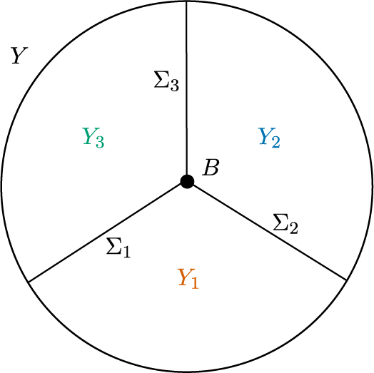
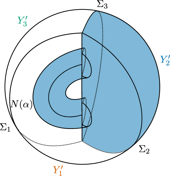
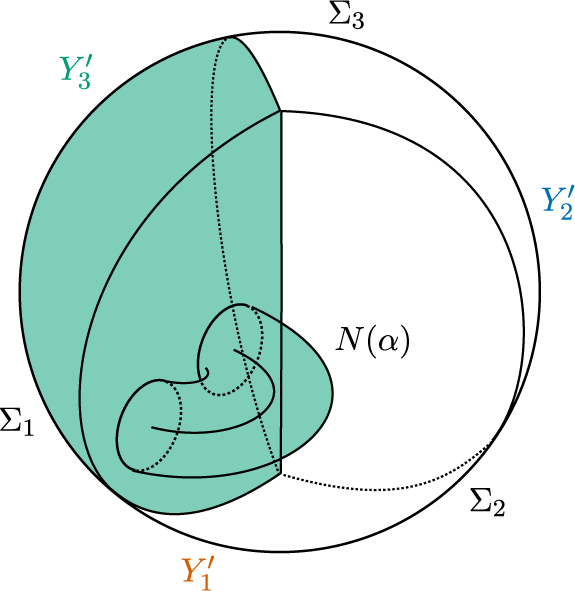
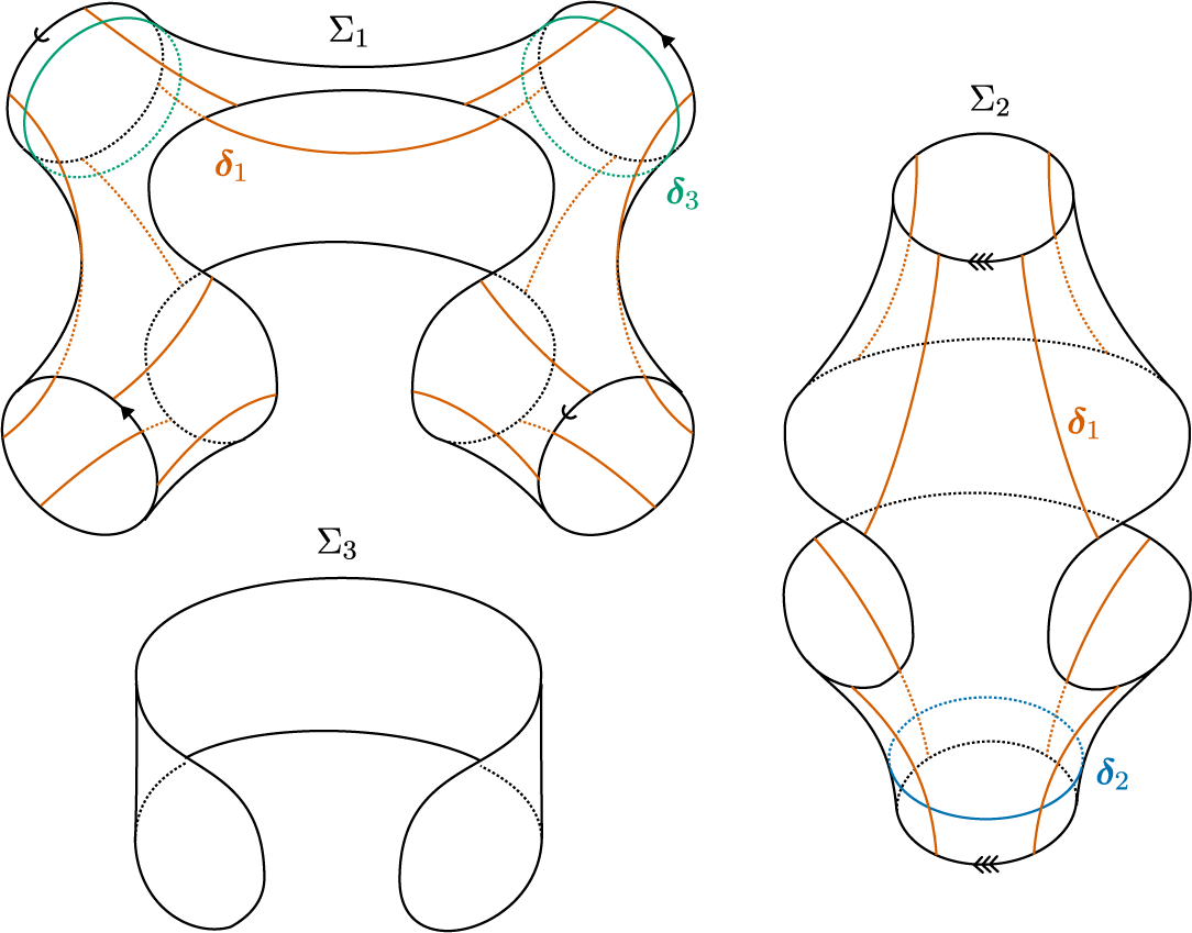

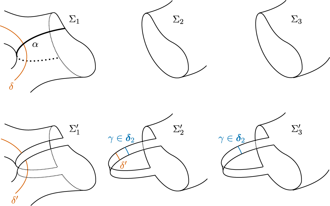
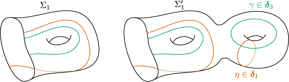
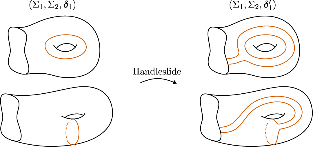


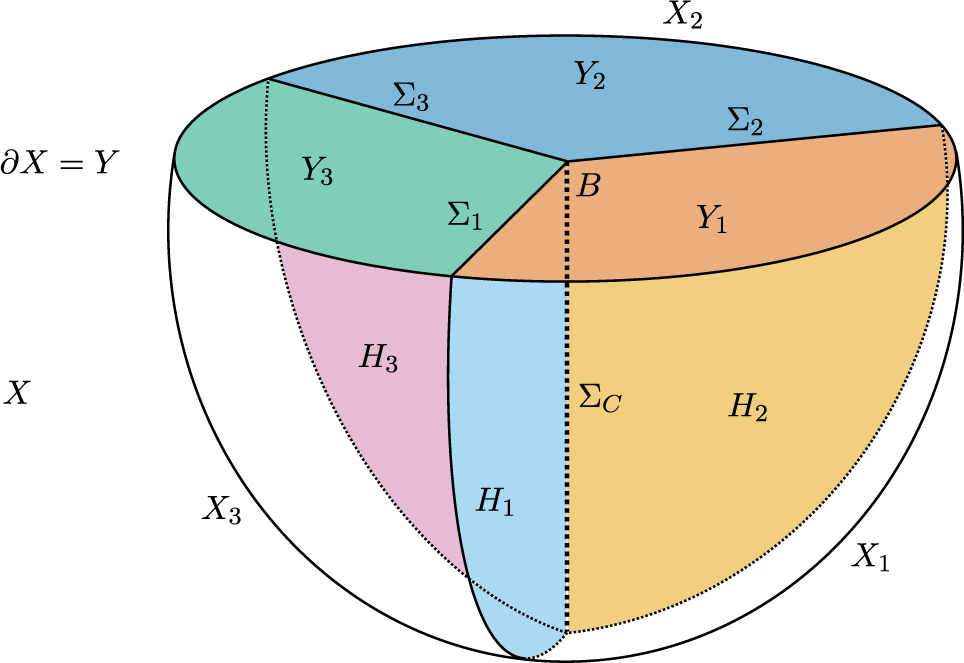
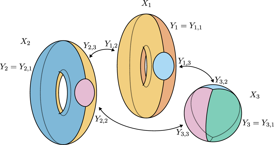
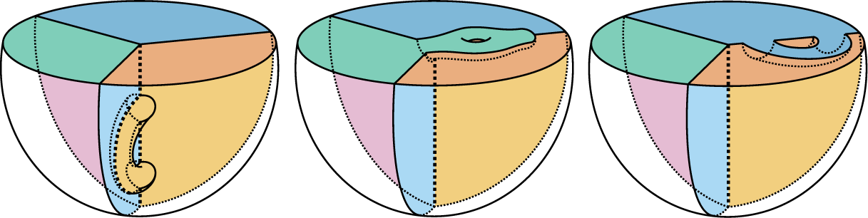
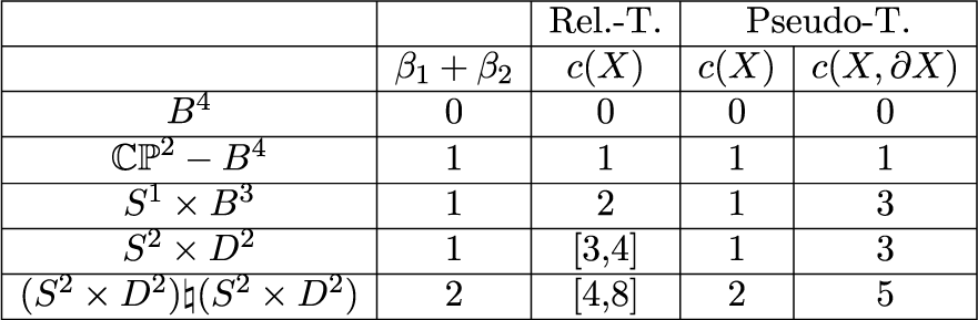
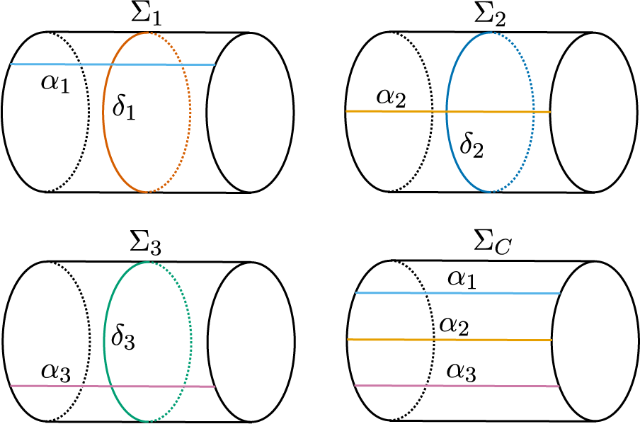

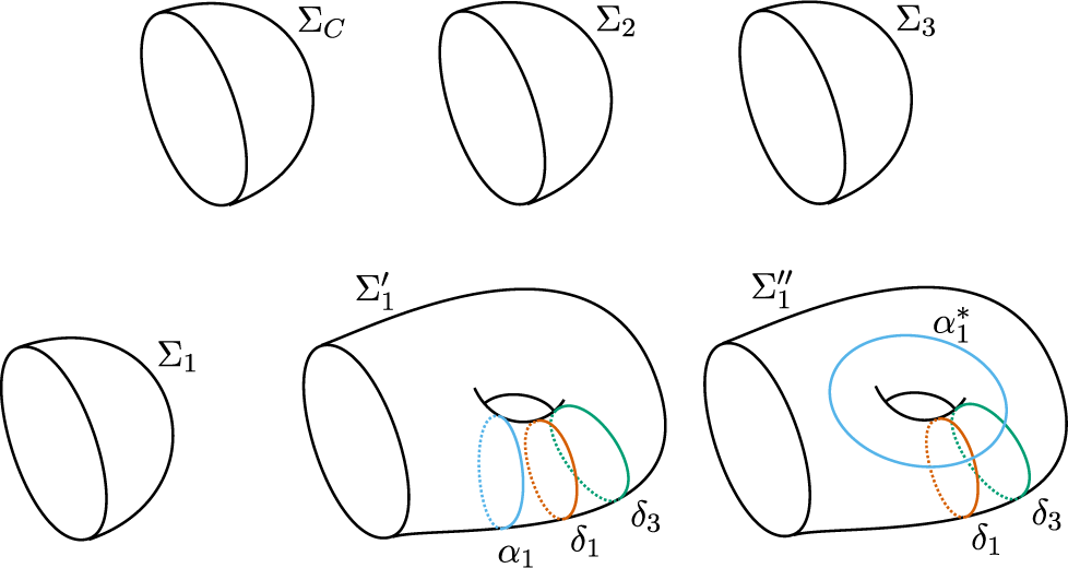

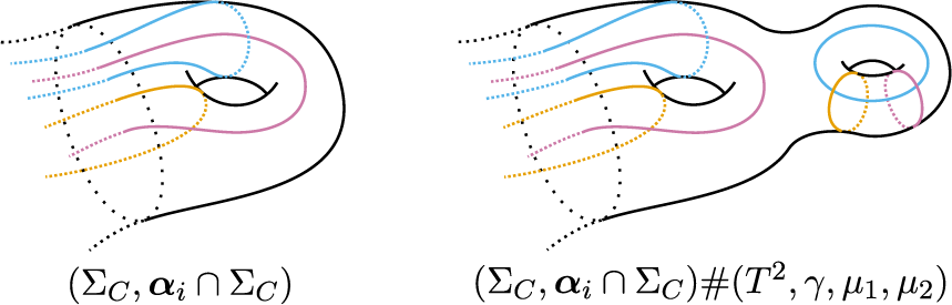
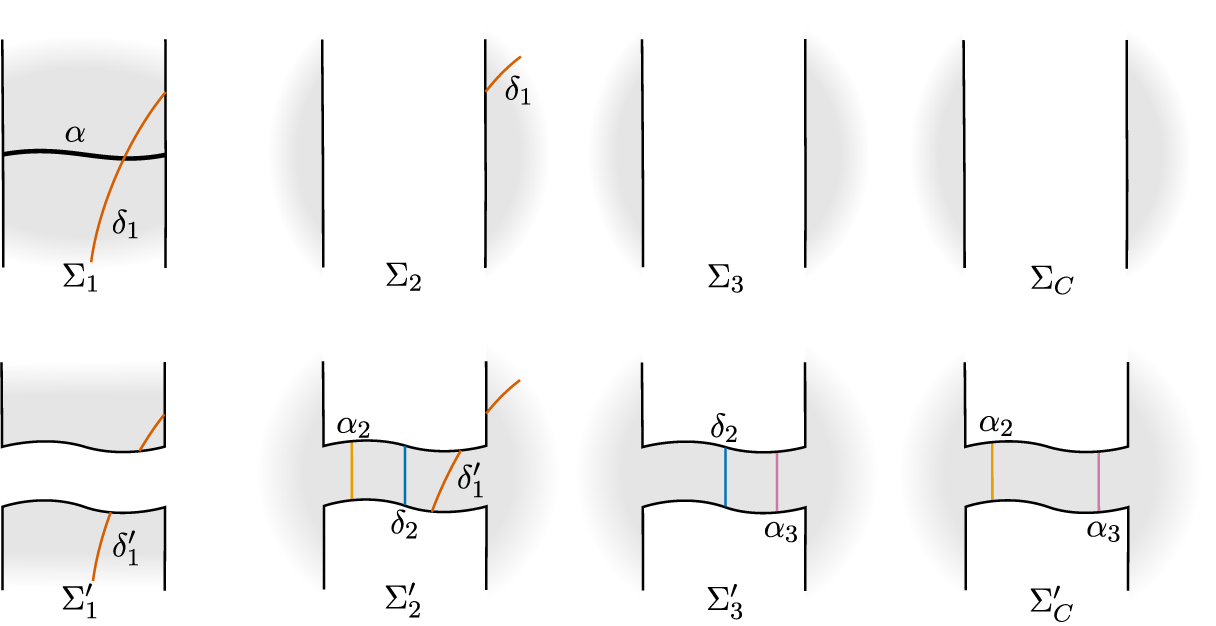
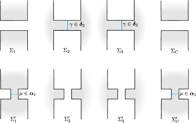
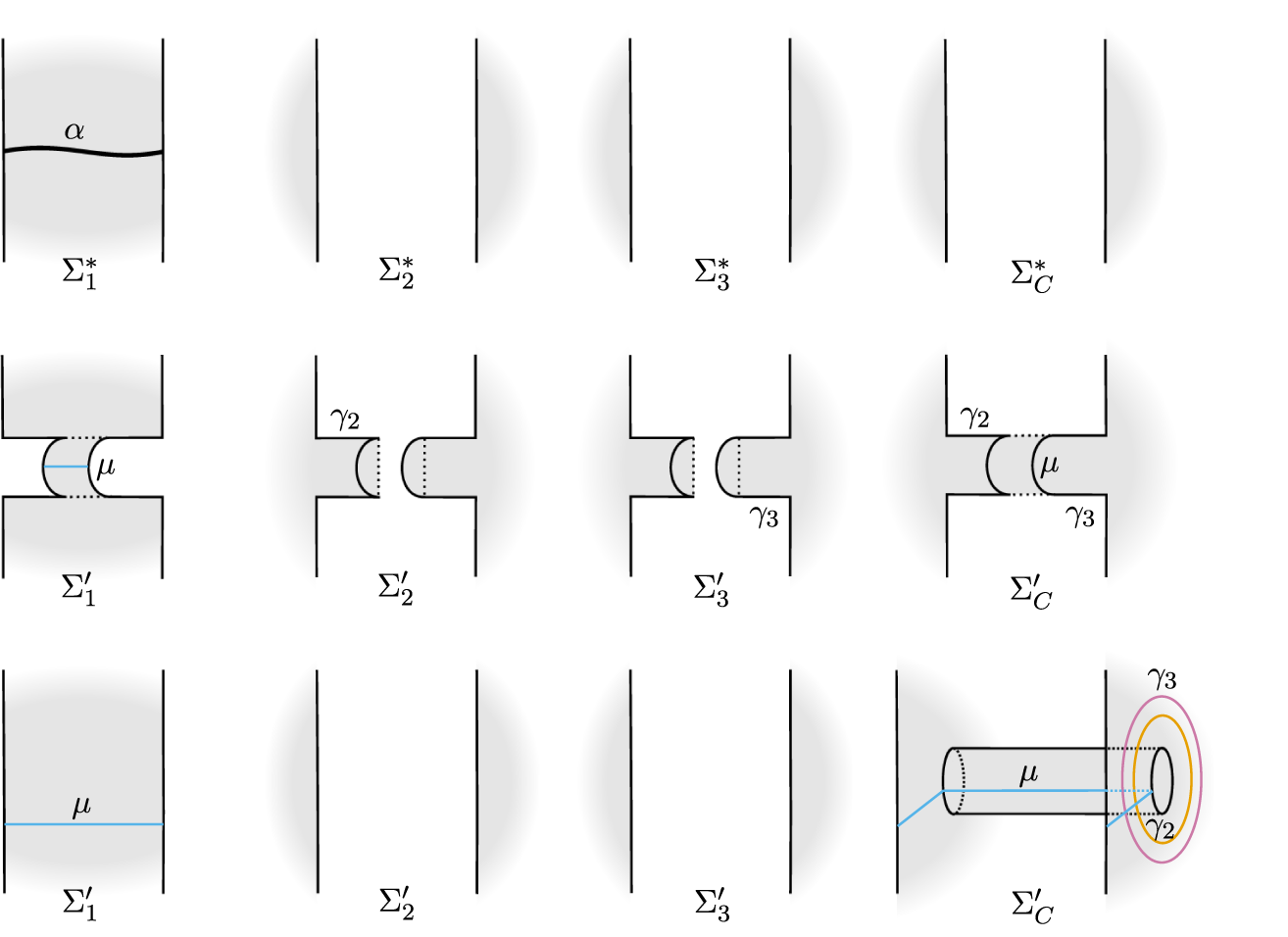
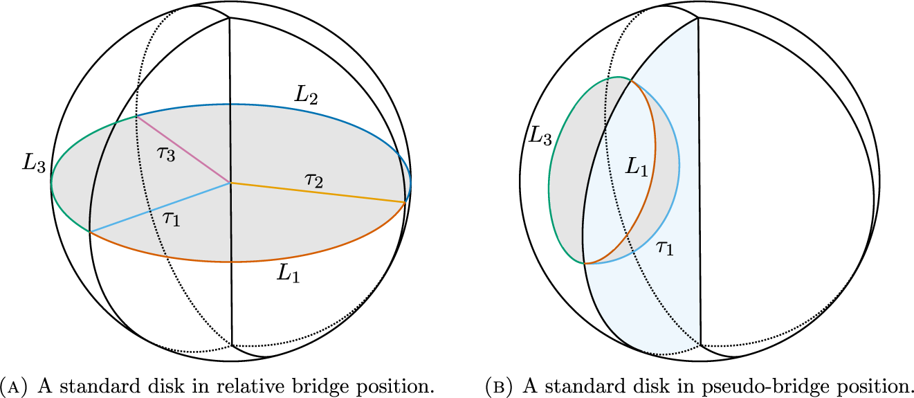

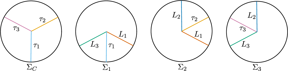

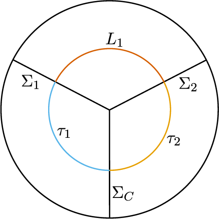

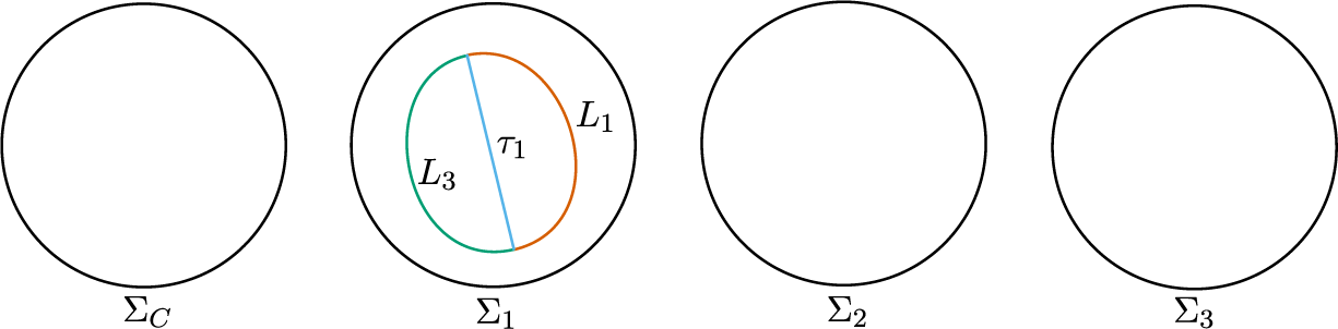

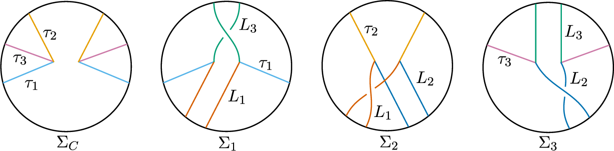


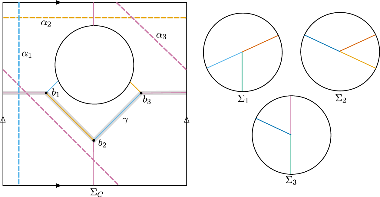

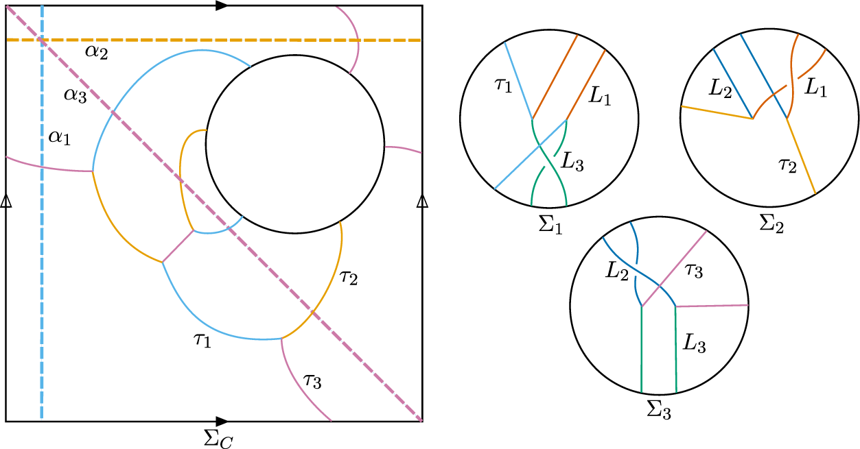


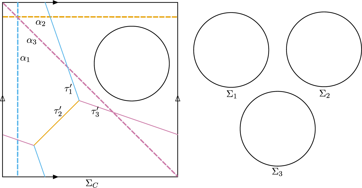


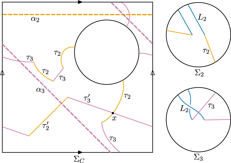


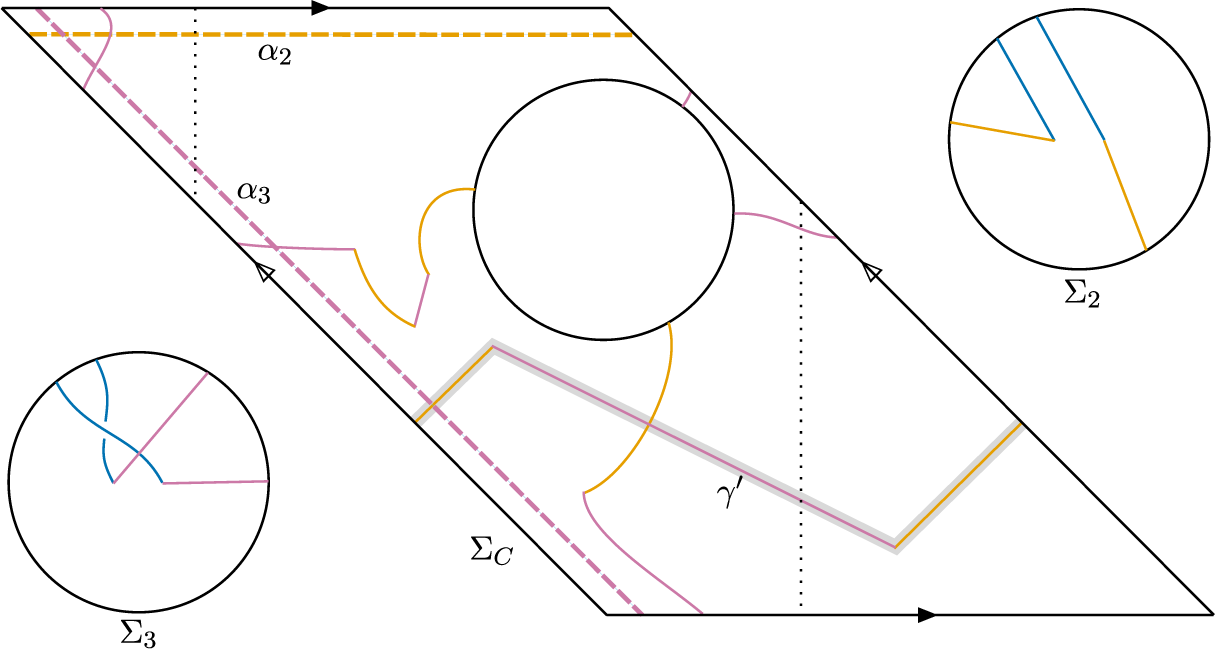


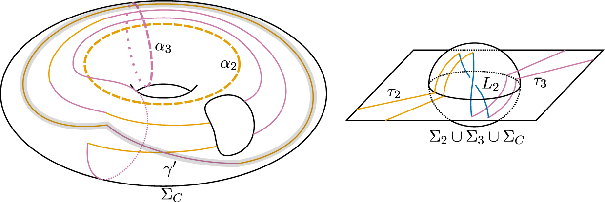


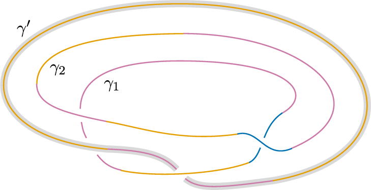


 Open access

