




No CrossRef data available.
Recognition of features of parts subjected to motion using ARTMAP incorporated in a flexible vibratory bowl feeder system
Published online by Cambridge University Press: 10 February 2006
Abstract
The recognition and identification of parts are important processes in modern manufacturing systems. Although machine vision systems have played an important role in these tasks, there are still challenges in performing these tasks in which parts may be in motion and subjected to noise. Using a flexible vibratory bowl feeder system as a test bed to simulate motion of parts subjected to noise, scanned signatures of part features are acquired using fiber optic sensors and a data acquisition system. Because neural networks have been shown to exhibit good pattern recognition capability, ARTMAP, a neural network that learns patterns under supervision, was incorporated into the feeder system. The pattern recognition capability of the feeder system is dependent on a set of parameters that characterized ARTMAP, the sampling rate of the data acquisition system, and the mean speed of the vibrating parts. The parameters that characterized ARTMAP are the size of an input vector, the vigilance, threshold value of the nonlinear noise suppression function, and the learning rate. Through extensive training and testing of the ARTMAP within the feeder system, it was shown that high success rates of recognition of parts features in motion under noisy conditions can be obtained provided these parameters of ARTMAP are appropriately selected.
Information
- Type
- Research Article
- Information
- Copyright
- 2006 Cambridge University Press
1. INTRODUCTION
To respond to the changes of market demands, manufacturing systems must be able to adapt to the production of a variety of products automatically, without manual changes to hard tooling. That is, the attributes of intelligence and flexibility must be built into manufacturing systems/subsystems. Manufacturing subsystems that perform the task of visual inspection or part/object identification must likewise exhibit the flexibility and adaptability required of intelligent and flexible manufacturing systems. Newman and Jain (1995) distinguish between inspection and recognition/identification. According to them, inspection is the process of determining if a product (e.g., part, object, or item) deviates from a given set of specifications to satisfy certain quality criteria (e.g., surface finish, geometric dimensions). Recognition involves the positive identification of an object (e.g., correct orientation of a part). It has been recognized that machine-based vision systems can identify materials and components, and locate and orient parts prior to assembly. These systems can perform inspection and measurement tasks during manufacturing processes and prior to shipment (Rosandich, 1997; Pham & Alcock, 2003). However, the automation of visual inspection has not kept pace with the automation of the manufacturing process (Newman & Jain, 1995). Rosandich (1997) suggested several factors that have limited the feasibility of such systems as follows:
- Installation of such systems often requires specialists' knowledge (e.g., illumination, cameras, computer interfacing, programming, and image processing).
- Installation often requires undesirable or inconvenient process changes (e.g., product line has to be stopped or separated or special equipment installed for illumination).
- Current systems lack flexibility, as each had to be custom designed for a specific task.
Similar limitations can be argued for machine-based vision systems used for recognition of objects.
Recognition of object or part features can be achieved using either machine vision (e.g., camera) or other sensors (e.g., fiber optics). Machine vision requires the integration of many aspects such as lighting, cameras, handling equipment, human–computer interfaces, and working practices, in addition to designing image-processing algorithms. Parts are fed from one station to another via conveyor, or fed in correct orientation for the downstream process using vibratory bowl feeders. Hence, real-time recognition of the part's features performed under motion would be a desirable capability in any part feeders. Although machine vision systems can recognize parts under motion, they would incur high computational overheads of image processing (e.g., motion analysis, correspondence of adjacent frames, etc.), which may be detrimental to achieving real-time performance.
This paper attempts to address these limitations inherent in machine vision systems by investigating how flexibility and on-line learning of features can be incorporated in an optical sensor-based system using neural networks to perform the task of feature recognition of parts in motion. To demonstrate the real-time recognition of parts under motion, the vibratory bowl feeder, a common parts feeding device in mass production is used. To facilitate automated flexible orientation of parts in batch production, the feeder has to accommodate a wide range of parts, has a short changeover time between parts, and delivers them in the appropriate orientation. To achieve flexibility, cleverly designed mechanical devices are attached to the traditional bowl feeder, which may reject a part in an undesired orientation back into the bowl, and machine vision or sensing devices is added as a means of determining part orientation. The nature of motion of the parts ensures that the sensing, and hence recognition, is subjected to noise.
Some researchers (Suzuki & Kohno, 1981; Cronshaw, 1980; Warnecke et al., 1991; Causey & Quinn, 1997) have employed machine vision (using CCD cameras), whereas others (Smals, 1985; Maul & Ou-Yang, 1987; Maul & Jaksic, 1994; Chua et al., 1997) have used sensor devices to capture the images of the feeding parts to recognize the parts orientation. In general, a recognition system is first taught to recognize the possible input orientations of a part in the learning/training mode in which patterns are stored in the computer system as reference signatures (i.e., templates). In the operation mode, the image acquired is compared to the reference signatures for identification of orientation (i.e., template matching). Using “template-matching” algorithms, the recognition system compares data acquired by the sensors with the prestored templates that represent the desired orientations of the parts. If a match occurs, the parts orientation can be determined. However, the disadvantage of the template-matching approach is that it is sometimes difficult to select a good template for each pattern class and define a proper matching criterion. Furthermore, this approach lacks flexibility in adapting to new parts requirements. When new parts are added due to changes in production demands, the process of retraining the system is required, leading to an increased down time.
Various types of neural networks have been used for applications that require feature recognition. Lankalapalli et al. (1997) have applied the self-organizing neural network ART2, which is based on adaptive resonance theory (ART; Carpenter & Grossberg, 1987a, 1987b) to the problem of feature recognition from a boundary representation (B-rep) solid model of nine different features. The results obtained indicate that the network has a significance potential for application to the problem of feature recognition. Sim et al. (2003) investigated the pattern recognition capability of three neural network models (namely, backpropagation, ART2, and ARTMAP) to identify the orientations of the parts moving in a programmable vibratory bowl feeder. Backpropagation (Rumelhart & McClelland, 1986) represents a class of neural networks that learn under supervised training but does not promote plasticity in its memory. ART2 is selected because it exhibits plasticity in its memory under unsupervised learning. ARTMAP (Carpenter et al., 1991a, 1991b) exhibits plasticity but lacks the ability to learn unsupervised. Of these models, ARTMAP is shown by Sim et al. (2003) to exhibit high recognition capability and flexibility in accommodating new parts without retraining. Hence, the flexibility that is sought in a parts feeder is achieved through the adaptability of ARTMAP in its pattern recognition performance of different parts features without the need of retraining.
The paper consists of the following sections. Section 2 describes the key characteristics of a family of neural networks referred to as ART and the parameters that characterize ARTMAP to achieve real-time recognition of parts' features. Section 3 describes the programmable vibratory bowl, the parts used in the experiments, and Section 4 describes the data acquisition and data preprocessing processes prior to parts recognition. Section 5 describes the details of two experiments conducted in terms of the organization of the training and testing data and the experimental procedures. The first experiment was conducted to optimize the ARTMAP parameters that have influence on the pattern recognition capability of the system. The second experiment was conducted to study the influence of sampling rates on performance of the fiber optic sensors in acquiring features of different moving parts. Section 6 presents the results of the two experiments, and Section 7 discusses the evaluation of the results in terms of ARTMAP parameters and the sampling rates on the pattern recognition capability of the vibratory bowl feeder system. Hence, the results obtained may provide some useful insights in solving a class of manufacturing problems that is characterized by pattern recognition of parts/objects in motion in real time and yet subjected to noise.
2. THE ARTMAP MODEL
ART, which was developed by Carpenter and Grossberg (1987a, 1987b), refers to a family of self-organizing neural architectures that cluster the pattern space and produce archetypal weight vector templates (Gurney, 1997). ART1 (Carpenter & Grossberg, 1987a), being the first member of the family, clusters only binary input patterns. ART2 (Carpenter & Grossberg, 1987b) overcomes the limitation of ART1 in that it can process analogue input patterns in addition to binary patterns. One of the main claims made for ART is that it overcomes the plasticity–stability dilemma in a natural way, so that the net is continually immersed in a training environment where there are no separate learning and testing phases (Gurney, 1997). In overcoming the plasticity–stability dilemma, ART2 is therefore able to retain existing patterns learned while learning new patterns.
The use of ART2 does not guarantee success in recognizing the orientations of the feeding parts. Several problems still exist. First, if the input patterns that belong to different categories are very similar, the only way to distinguish them is to set a high value for the vigilance parameter (ρ). However, a high ρ value causes the categories produced by ART2 to have less generalization ability, and hence, leads to poor recognition result. Second, when training ART2, a user cannot affect the learning process because of the self-organizing property. Therefore, a user cannot instruct ART2 how to learn the input patterns. This can result in misclassification of the input patterns.
Carpenter et al. (1991a) developed a supervised neural network architecture called ARTMAP. ARTMAP can autonomously learn to classify many arbitrarily ordered vectors into recognition categories based on predictive success. Hence, ARTMAP is also referred to as predictive ART network, and it is capable of fast, yet stable, on-line recognition learning and hypothesis testing, given a stream of input patterns (vectors). Although different ART modules can be incorporated into ARTMAP networks, here the choice of these modules is to facilitate on-line training of features of more than one part.
2.1. ARTMAP parameters
The ARTMAP model consists of three parts: ARTa, ARTb, and the map field. A control structure actively regulates learning and information flow. ARTa is used to receive training patterns, and ARTb is used to receive the target value of each training pattern. During training, a training pattern a will form a cluster in ARTa, although its target value b (a category of a) will also form a cluster in ARTb. The map field will be responsible for associating these two clusters (e.g., a belongs to the b category). During testing, an input pattern, which is received by the ARTa model, is assigned to the cluster made by training pattern a; the map field will associate this cluster to the cluster formed by b in ARTb as trained before. As a result, this input pattern is recognized by the ARTMAP model to be the b category.
In this study, ART 2-A (Carpenter et al., 1991b) was selected as the ARTa model, and the ART1 model was selected as the ARTb model. ART2-A adopts the fast learning version of ART2 to facilitate on-line training. In addition, the ART2 model differs from the ART1 network primarily in the implementation of the F1 layer (i.e., the input layer). Rather than a single structure of units, the F1 layer contains a number of sublayers that serve to remove noise, to enhance contrast, and to normalize an analogue input pattern. ART2, hence, is suitable for the application here because on-line learning subjected to noise is an important requirement of the pattern recognition task of the flexible and programmable vibratory bowl feeder. According to the training process of the ARTMAP model, different target values must be assigned to different clusters of ARTb to represent each category (i.e., the orientation of the part). Therefore, the clusters formed in ARTb must be very specific. As a result, the vigilance parameter ρb must be very high. The value of ρb is set to 0.999, which implies that the only parameter that governs the training and testing of the ARTb model of ARTMAP (represented by ART1) is fixed. Only the parameters of the ART 2-A model, (represented by the ARTa model of ARTMAP), can be changed when the performance of ARTMAP is studied.
2.2. ART 2-A parameters
In defining an ART 2-A model, the three parameters that can be changed during training, and testing phases are α, θ, and ρ. As a fast learning mode is desirable for rapid recognition of parts, the learning rate (β) is set to 1.
2.2.1. Parameter α
Parameter α corresponds to the initial value of the components in ART 2-A F1 (input layer) to F2 (competitive layer) weight vector. The constraint for α is

, where M is the dimension of the input vector of the ART 2-A model (i.e., the number of input nodes of the ART 2-A model). Setting α close to

biases the ART 2-A model toward the selection of an uncommitted node over committed nodes that only partially match the training pattern. That is, when α is high, the ART 2-A model biases to form more clusters to represent the same training patterns compared to the number of clusters used to train the model when α is low.
2.2.2. Parameter θ
Parameter θ corresponds to the threshold value of the nonlinear noise suppression and contrast enhancement function that is applied in the preprocessing layer F0 of the ART 2-A model. The constraint for θ is

, where M is also the dimension of the input vector of the ART 2-A model. The value of θ is critical to the contrast enhancement and noise suppression of the preprocessing layer. Subthreshold signals of the normalized input pattern are set to zero, whereas suprathreshold signals are amplified by the subsequent normalization step at the top F0 layer.
2.2.3. Parameter ρ
Parameter ρ corresponds to the vigilance parameter value of the ART 2-A model. The constraint for ρ is 0 ≤ ρ ≤ 1. During training, the value of ρ determines if a training pattern belongs to a category that has already been trained or it represents a new category. During testing, the value of ρ determines whether an input pattern belongs to one of the trained categories of the ART 2-A model, or it is an unrecognized pattern.
In the experiments described below, the value of these three parameters will be varied within the allowable range to see how they affect the success rate of the ARTMAP model.
3. THE FLEXIBLE VIBRATORY BOWL FEEDER SYSTEM
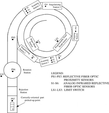
Here, the description of the programmable vibratory bowl feeder and the details of parts used in the experiments provide background knowledge for the experiments described in Section 5. Figure 1 shows the schematic diagram of the flexible and programmable vibratory bowl feeding system. It has three subsystems as follows:
- a vibratory bowl feeder,
- a sensing cum recognition subsystem using ARTMAP neural network, and
- a programmable logic controller (PLC).

A schematic diagram of the feeding system.
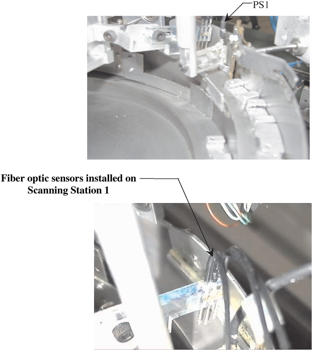
Parts poured into the vibratory bowl feeder move along the track of the feeder. After passing through the wiper blade station (LS1) and programmable width station (LS2), only parts of certain width and height are allowed through to the first singularization station (PS1; see Fig. 2), which ensures that only one part at a time proceeds to the scanning station 1 (PS2). At PS2, each part passes under three analogue sensors (i.e., S1, S2, S3; see Fig. 2). The analogue signals of the part's surface are sent to the data acquisition card. These will be converted into digital signals, which are then processed by the pattern recognition subsystem that is implemented here using the ARTMAP neural network. Upon recognizing the part's orientation, a signal will be sent by the computer to the PLC. If the part is in the wrong orientation, the PLC will send a signal to the flipping station (PS3) to flip the part. The part then progresses to the second singularization station (PS4) and the second scanning station (PS5) to validate if the part is in the correct orientation by passing under three fiber optic sensors (i.e., S4, S5, and S6). The rotation station (PS6) will correct an incorrectly orientated part before it moves to PS7 for the next process action.

The singularizing station and scanning station 1. [A color version of this figure can be viewed online at www.journals.cambridge.org]
4. DATA ACQUISITION AND PREPROCESSING
This section gives an insight into the difficulties faced in data acquisition, as well as the steps taken to acquire parts' signatures that may be subjected to noise and likely variations in the loading of the bowl feeder as parts leave the feeder.
4.1. Feeding parts
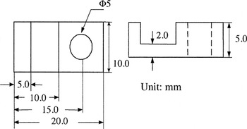
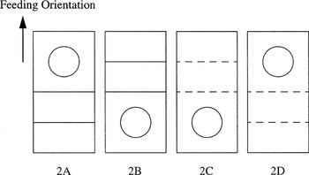
Although two similar parts (parts 1 and 2) have been used for the experiments reported in Sim et al. (2003), here only part 2 has been used. Part 2 has the dimensions given in Figure 3. It has 24 possible orientations when traveling on the track of the vibratory bowl feeder. After passing through the flexible orientating devices (LS1 and LS2), only four of these orientations are permissible. These orientations are to be recognized by the neural network system (i.e., the ARTMAP model). Figure 4 illustrates these four orientations and the corresponding representation codes. Among these orientations, B1 is the desired orientation of part 2.

Feeding part 2 used in the experiments.

Four feed orientations that ARTMAP should identify.
4.2. Calibration of the analogue sensors
The scanned signature of a part serves as input to the neural network model whose primary function is to recognize the orientation of the part. Hence, the quality of the scanned signature is very important to the pattern recognition capability of the neural network model. If the scanned signature cannot depict the part's surface correctly, the orientation determined by neural networks will be incorrect. Therefore, the purpose of calibration is to adjust the sensors to the correct settings so that they produce the same readings for a given height of a part. The calibration can be achieved through a program that gives on-line readings of the analogue channels.
Part 2, with a flat surface of a height of 5 mm, is first placed under the sensors. The range of A/D conversion of the data acquisition card is set from −5 to +5 V. The sensors are calibrated by either turning the sensitivity notches or adjusting the positions of the sensor tips until the reading of all three sensors just reached 5 V. This process of calibration is repeated for all the features of the part (i.e., the part's flat surface, the groove, and the through hole).
4.3. Settings of the data acquisition card
The pacer rate (p) of the data acquisition card is given by

where C1 and C2 are the user programmable parameters of the card. Their values range from 2 to 65,535.
Different pacer rates can result in different data quantity in a given time. If the rate is too high, a large signature data file will be input to the neural network. This tends to increase the computation time of the neural network, which may impede the on-line pattern recognition process. If the rate is too low, the signature acquired may lose some important features of the part.
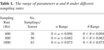
Because the sampling rate can have a significant influence on the pattern recognition of the neural network, its influence on input data to the ARTMAP was investigated. When the sampling rates change, the size of the input data also changes, resulting in a different number of input nodes for the ARTMAP model. This will affect the range of α and θ according to the constraint formula given in Sections 2.2.1 and 2.2.2. In the experiments described below, different sampling rates were used to acquire the parts' surface signatures. Table 1 shows the sampling rates, the corresponding number of sampling per sensor, together with the range of values for parameters α and θ under different sampling rates.
The range of parameters α and θ under different sampling rates

4.4. Data acquisition
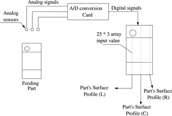
A part's surface is scanned for its surface signature by the scanning station (i.e., PS2), which consists of three fiber optic sensors (i.e., S1, S2, and S3). Figure 5 illustrates the scanning of the parts using part 1 as an example. Scanning begins when each sensor senses the leading edge of the parts and the data acquisition card begins the A/D conversion. When the part passes through the scanning station, the analogue sensors receive the reflected light from the part, and convert the light signal to an electrical signal depending on the intensity of the light reflected. The section with a greater thickness will reflect a stronger light signal back to the sensor because it is closer to the sensor. Therefore, the sensor transforms a higher voltage for this section of the part to the data acquisition card. Through this method, scanned signatures are to depict the profile of a part's surface. As each sensor acquires 25 data, the data acquisition card performs 75 times A/D conversion. Hence, the input vector to a neural network model is fixed at 75.

The scanning process.
4.4.1. Scanned signature
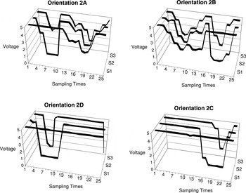
Figure 6 shows the scanned signatures of different orientations of part 2. From the figure, it can be seen that the scanned signatures depict the features of a part (i.e., the groove and the through hole). However, the signatures are not stable even for the same height of a feeding part. This is due to the vibration of the bowl feeder that imparts a forward and upward flight to a part moving along the bowl's track.

Scanned signatures of part 2 in different orientations.
4.4.2. Problems of data acquisition
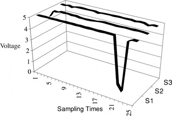
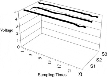
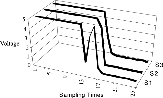
Due to the vibratory agitation of the bowl feeder, Boothroyd et al. (1982) show that a part can be subjected to different states of motion during each vibration cycle (i.e., slide forward, slide backward, and bounce). Although not every state occurs in each cycle, the different motion states will definitely affect the scanned signature. For example, the bounced state tends to give rise to unstable signatures. Hence, due to the presence of the unstable signatures acquired during the scanning process there is a need for ARTMAP to perform parts recognition under such noisy conditions. Although there are many types of scanned signatures that can possibly be acquired by the sensors, here three different types of scanned signatures are identified for the purpose of highlighting the need to preprocess the data before they are used as inputs into the neural network model (see Figs. 7, 8, and 9).
Figure 7 shows the scanned signature of a feeding part (part 1) that passed through the scanning station at an ideal speed. The ideal speed is defined as a speed that gives good correlation between the sampling rate and the parts' speed. If the sample rate is 400 Hz, then this occurs when the whole part will just pass through the scanning station at the end of 25 times A/D conversion.

A scanned signature of part 1 where the speed is ideal.
Figure 8 shows the scanned signature of part 1 in the same orientation (as that shown in Fig. 7) at a speed that was too slow. It can be seen that the part's signature is incomplete (i.e., the hole in the left end of the part's surface cannot be captured). Therefore, slow speed often causes the loss of the part's feature.

A scanned signature of part 1 where the speed is too slow.
Figure 9 shows the scanned signature of part 1 in the same orientation at a speed that was too fast. Comparing Figure 9 with Figure 7, it can be seen that the size of the hole is reduced. In Figure 7, the two zeros representing the hole feature, but only one zero in Figure 9. Hence, the scanned signature does not depict the part's actual surface. In general, a fast speed reduces the part's scanned signature.
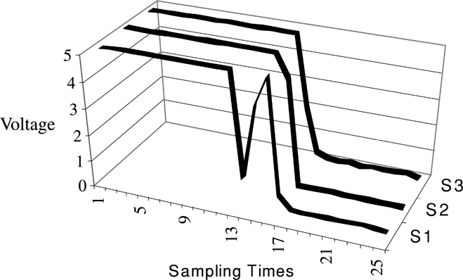
A scanned signature of part 1 where the speed is too fast.
In general, parts traveling at a fast speed or slow speed will present difficulties in recognizing the part's orientation by the neural network. Hence, there is a need to ensure that the scanned signatures should be as similar as possible to that achieved in the ideal speed.
4.5. Data preprocessing: Normalization of the scanned signature
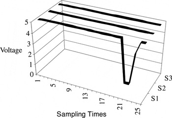
To overcome the problems described above, data preprocessing of the scanned signatures called normalization was performed. A more general solution has been provided by Maul and Jaksic (1994) for parts that are contiguous and overlapping traveling under different parts velocities using two sensor algorithms and a variable called “precision” that is dependent on the part's length in the control program. Here, normalization is used to expand the short scanned signature proportionally to the correct number of data readings. For example, in Figure 9, the first 15 data in the scanned signature are considered as representing the feature whereas zero readings from the 16th data onward can be considered as errors as they do not represent the real feature. The portion of the scanned signature that has erroneous readings will be deleted, and the useful portion expanded proportionally to the last data (i.e., 25th value). Figure 10 illustrates the normalized parts signature of the scanned signature shown in Figure 9. However, the normalized signature may not always have the fidelity of the original scanned signature.

A scanned signature of part 1 after normalization.
Unfortunately, normalization can only be applied for the parts traveling at high speed. It is ineffective for the case where the scanned signature is incomplete (shown in Fig. 8). One of the ways to solve this problem is to increase the number of the A/D conversion, so that normalization can be applied to parts with the lowest speeds. This speed can be achieved by increasing the feeding speed of vibratory bowl feeder from zero to a value when one of the parts begins to move.
5. DESCRIPTION OF THE EXPERIMENTS CONDUCTED
From discussion in Sections 2 and 4, it can be seen that the pattern recognition capability of the flexible vibratory bowl feeder system is dependent on two major factors:
- the parameters that influence the formation of clusters in the structure of ARTMAP and
- the rate of the data acquisition process (i.e., the sampling rate) and the influence of the mean speed of the parts in the bowl feeder.
Hence, the purpose of the two experiments described here was to investigate the influence of these factors on the pattern recognition capability of performance of the system. The two experiments conducted are referred to as experiment A and experiment B.
5.1. Organization of training and testing set
To investigate the influence of the different parameter settings on the success rates of the ARTMAP model, the scanned signatures of part 2 were used to train and test the ARTMAP model. The ARTMAP model is trained to recognize four desirable orientations of part 2 (i.e., 2A, 2B, 2C, and 2D, shown in Fig. 4).
5.1.1. Training and testing sets organization
To investigate the effects of the parameters, all other conditions should remain unchanged during the experiments. Therefore, the same training and testing set were required to train and test the ARTMAP model under different parameter settings. The size of the training set was 20; the data files that comprised the training set are 2A1–2A5, 2B1–2B5, 2C1–2C5, and 2D1–2D5. The testing set consists of the training set and all other scanned signature data files for each orientation.
5.2. Experiment A
The influence of the parameter α on the pattern recognition of ARTMAP has been investigated by others (Carpenter et al., 1991a). As mentioned in Section 2, a high α value biases the ARTMAP model to form more clusters in its ARTa model to represent the same training patterns. The purpose of experiment A, therefore, is to investigate the value(s) of α in the ARTMAP model(s) that will achieve an optimal pattern recognition capability.
5.2.1. Procedure of experiment A
1. One hundred signatures per orientation of part 2 were recorded at PS2 of the vibratory bowl feeder and each signature was saved as a data file in the computer. The sampling rate used was 600 Hz.
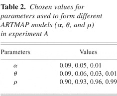
2. The values of the parameters (α, θ, and ρ) that characterize ART 2-A (the ARTa model of ARTMAP) were selected as given in Table 2. Each ARTMAP model was trained with the training set as described in Section 5.1.
3. The recognition performance of the trained model was evaluated using the testing set. The success rate (SR) was calculated as follows:

4. From the results, the effect of parameters on the recognition performance was analyzed.
Chosen values for parameters used to form different ARTMAP models (α, θ, and ρ) in experiment A

5.3. Experiment B
The purpose of experiment B is to study the effect of parameter θ and the sampling rate on the performance of the ARTMAP model, hence, to find the optimal values of these two parameters.
5.3.1. Procedure of experiment B
- One hundred signatures per orientation of part 2 were recorded from the scanning station, PS2 of the vibratory bowl feeder for each of the sampling rates (i.e., 800 and 1000 Hz), and each signature was saved as a data file in the computer. In this experiment, the data files recorded in experiment A at 600 Hz were also included.
- For each sampling rate, the same set of data files was used for training and testing the ARTMAP models. The size of the training set was 20; the data files that comprised the training sets are 2A1–2A5, 2B1–2B5, 2C1–2C5, and 2D1–2D5.
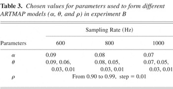
- A range of values for the parameters θ, ρ, and α was
selected as given in Table 3 for ART 2-A (the
ARTa model of ARTMAP) to form different ARTMAP models.
The values of α chosen were near the optimal value found in experiment
A. Hence, in experiment B, the value of α for each sampling rate
selected is close to
(i.e., α = 0.07, 0.08, and 0.09). Each ARTMAP model was trained with the training set organized in step 2. The trained models were tested with the testing set, which has the same sampling rate as the training set. The success rates of recognition were calculated. From the results, the effect of parameters θ, ρ, and sampling rate were analyzed.

Chosen values for parameters used to form different ARTMAP models (α, θ, and ρ) in experiment B

6. EXPERIMENTAL RESULTS
6.1. Results of experiment A
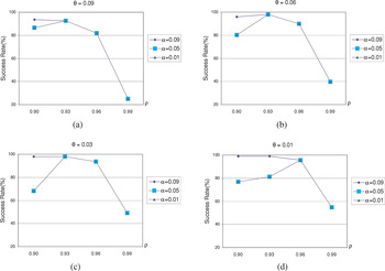
A total number of 48 ARTMAP models was configured using different combinations of the chosen values of the parameters α, θ, and ρ; these parameters can have a significant influence on the performance of ARTMAP. The success rates of parts recognition for these 48 ARTMAP models are illustrated in Figure 11.

The success rate of ARTMAP models composed of different α values. [A color version of this figure can be viewed online at www.journals.cambridge.org]
From Figure 11, it can be seen that for all values of θ and ρ, the success rates of ARTMAP models that have lower α values (α = 0.05, α = 0.01) were not always greater than the models that have a higher α value (α = 0.09). When the value of ρ was increased beyond 0.96, the success rates appeared to be the independent of α for a given value of θ. For each combination of ρ and θ, where θ > 0.01 and ρ > 0.93, it can be observed that the success rates of the ARTMAP models were the same for all the values of α.
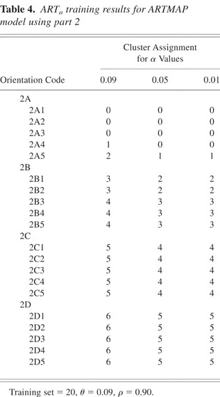
The reason why the value of α can affect the success rate of ARTMAP is due to its influence on the training result of the ARTa model when subjected to the same training set. As discussed in Section 3, ARTa models with high values of α form more clusters to represent the same training patterns compared to trained models with low values of α. To understand the influence of α, the training of ARTa in three ARTMAP models with different parameter setting were studied. For these models, the values of θ and ρ were set at 0.09 and 0.9, respectively, but the values of α were varied. Table 4 shows the training results of ARTa in the three ARTMAP models.
ARTa training results for ARTMAP model using part 2

From Table 4, it can be seen that the ARTa model formed seven clusters when α = 0.09, compared to six clusters when α = 0.05. The F2 layer of the ARTa model is a competitive layer in which only the uninhibited node with the largest net input has a nonzero activation: that is, the node with the largest input will be chosen to learn the training pattern. During training, when the training pattern 2A4 (see Table 4) was processed in the F2 layer, the ARTa model will choose an uncommitted node rather than a previous committed node (cluster 0) to learn the training pattern when α = 0.09. However, when αs were set to 0.05 or to 0.01, the ARTa model chose the previous committed node (cluster 0) to learn the training pattern 2A4, thus forming less clusters after training.
Different training results led to different testing results. Figure 11a shows the different success rates of the three ARTMAP models. From the testing results, it can be seen that a high α value produces a high success rate. That is, for the same values of ρ and θ, the formation of more clusters in the ARTa model is indicative that the network is subjected to better training for a given training set. From Table 3, because the training resulted in the same number of clusters being formed when α = 0.05 and 0.01, the success rates for the two ARTMAP models were also the same. It can also be seen that α tends to loose its influence on training when the value of vigilance parameter ρ was increased. This is because when the value of ρ increases, the criteria that the ARTa model commits a node to learn new training pattern becomes stricter. When training an ARTMAP model with a low α value, the selection of the committed node to learn a new training pattern will be rejected by the reset process of the ARTa model because of the increased ρ value. The results shown in Figure 11 indicate that setting α close to its upper constraint value

can result in a better success rate of the ARTMAP model in this feeding system for values of ρ < 0.93.
6.2. Results of experiment B
From Table 3, it can be seen that there were three training and testing sets organized for three different sampling rates (i.e., 600, 800, and 1000 Hz, corresponding to α = 0.09, 0.08, and 0.07, respectively). Hence, for each sampling rate, values were chosen for parameters θ and ρ to form 40 different ARTMAP models. To compare the recognition performance of these 40 models, each of these ARTMAP models was trained and tested by the same training and testing set, respectively.
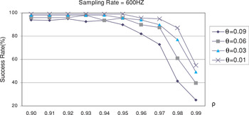
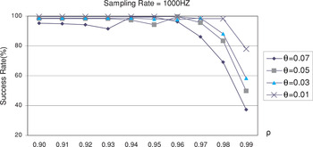
Figures 12 and 13 show the success rates of these 40 ARTMAP models for sampling rates of 600 and 1000 Hz, respectively. It can be seen that the trend of success rates of the ARTMAP models for each sampling rate has something in common. First, the success rate decreases when the value of ρ increases close to 1.0, its upper constraint value. Second, the highest success rate always occurs when θ = 0.01. Third, the success rates of ARTMAP models with higher θ values are always lower than that of ARTMAP models with lower θ values for the given ρ value.

The success rate of ARTMAP models composed of different θ and ρ values (sampling rate = 600 Hz, α = 0.09). [A color version of this figure can be viewed online at www.journals.cambridge.org]

The success rates of ARTMAP models for different values of θ and ρ (sampling rate = 1000 Hz, α = 0.07). [A color version of this figure can be viewed online at www.journals.cambridge.org]
It can be seen that increasing the sampling rate did not increase the success rate significantly, because ARTMAP models can achieve high success rate for each sampling rate. However, increasing the sampling rate does increase the stability of the scanned signatures of the feeding part. This can be seen from the success rates when ρ = 0.99; the higher sampling rate always produce a higher success rate than the lower sampling rate. Hence, stable scanned signatures may indicate that the success rate of the ARTMAP model is less affected by the parameter settings.
Figures 12 and 13 show that the success rates decrease when ρ tends to the value of 1.0. This can be explained by the fact that the generalization ability of each cluster formed in the ARTa model decreases when ρ increases. Therefore, less testing patterns can be correctly recognized for a higher ρ value if the testing patterns that belong to the same cluster are not very stable. Because of the vibration of the feeding system and the manufacturing tolerance of the feeding parts, it is expected that differences do exist among the scanned signatures even for the same orientation. Hence, if clusters that represent the part's orientations do not exhibit sufficient generalization ability, the success rate will be affected.
However, not every increase of the ρ value leads to a decrease in the success rate. From Figure 12, it can be observed that the success rates of the ARTMAP models remain fairly constant for certain range of ρ (0.9–0.94). This is due to the similarity of the input patterns that belong to the same cluster. If the input patterns are sufficiently similar it can be seen that over a certain range of values of ρ, the success rates do not vary significantly. However, when ρ is increased close to its maximum limit of 1, the generalization ability of the network tends to decrease. When this happens, any difference between training and testing patterns will cause error for the ARTMAP model. Therefore, the success rate decreases dramatically. From Figure 12 it can be seen that the success rates of the ARTMAP models tested for different ρ values have some fluctuation when θ = 0.09 and 0.06. The same inference can be derived for Figure 13 when θ = 0.07 and 0.05. As discussed in Section 2, the ARTa model tends to form more clusters when ρ is increased.
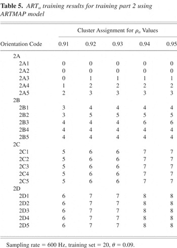
To explain the influence of ρ on the number of clusters formed, the training results of ARTa for the success rates shown in Figure 12 when θ = 0.09 were tabulated in Table 5 for different values of ρ. From Table 5, it can be seen that the ARTa model formed seven clusters when ρ = 0.91 compared to eight clusters when ρ = 0.92. Due to the increase in the number of clusters formed, the success rate of the ARTMAP model when ρ = 0.95 is lower than that of the model when ρ = 0.93. Hence, it can be seen that as ρ tends to be 1, the success rates for the ARTMAP models shown in Figure 12 tend to decrease.
ARTa training results for training part 2 using ARTMAP model

7. DISCUSSION
Experiments A and B investigated the effect of the parameters of the ARTMAP model on the pattern recognition capability as measured by the success rates. The experimental results show that to achieve a better success rate of pattern recognition by the ARTMAP model, the α value should be set close to

, and the θ value should be set very small such as 0.01 for each sampling rate. Hence, for given values of α and θ, the results indicate that an optimal value of the vigilance parameter ρ can be selected. For example, in Figure 12, when θ = 0.01 and α = 0.09, the highest success rate of the ARTMAP model was 99% was achieved when ρ values vary from 0.90 to 0.95. To select an optimal value for ρ, there is a need to consider the two types of errors in the ARTMAP models, namely the misclassified error and the unrecognized error. The misclassified error occurs when a certain orientation of the feeding part is recognized by the ARTMAP model to be that of another orientation. For example, a part moving in orientation 2A may be recognized by the ARTMAP model to be moving in orientation 2C. The misclassified error can cause the feeding parts to remain in the undesired orientation when they exit the feeding system, making the feeding system unreliable. The unrecognized error occurs when the part's orientation cannot be recognized by the ARTMAP model. The unrecognized error will cause the rejection station to reject the feeding part, resulting in recirculation later. Therefore, it will not contribute to the error of the feeding system.
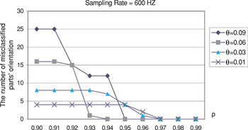
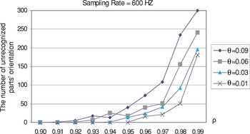
For these reasons, the error of the ARTMAP model should consist only of the unrecognized error. In this case, the error of the ARTMAP models, which were tested in experiment B, was investigated. Figures 14 and 15 illustrate the number of misclassified errors (Fig. 14) and unrecognized errors (Fig. 15) for a sampling rate of 600 Hz.

The misclassified error distribution of ARTMAP models using different values of θ and ρ (sampling rate = 600 Hz, α = 0.09). [A color version of this figure can be viewed online at www.journals.cambridge.org]

The unrecognized error distribution. [A color version of this figure can be viewed online at www.journals.cambridge.org]
From these figures it can be seen that the misclassified error decreases when the value of the ρ value increases, whereas the unrecognized error increases when the ρ value increases. This is because when ρ is increased, the clusters formed in the ARTa model become more specific, hence causing the misclassified error to decrease and the unrecognized error to increase. When the ρ value is increased to a certain value, the misclassified error decreased to zero, and only the unrecognized error is left. However, when the ρ value was too high (i.e., close to 1), the unrecognized error becomes very large because the generalization ability of the clusters formed in the ARTa model becomes almost nonexistent. Therefore, the optimal ρ value for maximum recognition is achieved when the misclassified error approaches zero. From Figures 11, 12, 13, 14, and 15, it is reasonable to infer that this optimal value for ρ is 0.96 or 0.97. For example, when the sampling rate is 600 Hz, α is 0.09 and θ is 0.01; as shown in Figure 12, the maximum success rates were achieved when ρ = 0.96 and 0.97, and the misclassified error as indicated in Figure 14 is 0. Although the success rate is not the highest, it can ensure the reliability of the feeding system. Therefore, the optimal ρ value for the ARTMAP model of the feeding system should be set to 0.96 or 0.97.
8. CONCLUSION
By using a flexible and programmable vibratory bowl feeder as the testbed for the identification and orientation of parts, this paper has demonstrated that ARTMAP is an appropriate neural network for the on-line pattern recognition of moving parts with varying mean speeds whose patterns are time sensitive and subjected to noise. ARTMAP that learns under supervision incorporates ART2-A as the ARTa model, which receives training patterns, and ART1 as the ARTb, which receives the target value of each training pattern. It has been shown that the pattern recognition capability of ARTMAP is related to the parameter settings of ART2-A through α, θ, and ρ.
The scanned signatures of the moving parts were acquired through optical sensors using varying sampling speeds that have a direct influence on the size of the input vector to the neural network model (i.e., ARTMAP). The size of the input vector is governed by the parameter α. From the results of the experiments, it has been shown that the values for parameter α should be set as close to

as possible. Because the scanned signatures are subjected to noise, the noise suppression and contrast enhancement feature of ART2-A governed by θ should be set a low value (e.g., 0.01) for a given sampling rate. Under these settings of α and θ, the optimal value for the vigilance parameter is from 0.96 to 0.97 to achieve high success rates for pattern recognition.
It is reasonable to suggest that similar applications that involve the task of pattern recognition of moving parts can benefit from the use of ARTMAP as a neural network model for pattern recognition provided appropriate values are chosen for parameters that govern the size of the input vector α, the noise suppression and normalization of input vector θ, and the vigilance parameter ρ that discriminates between different classes of patterns. If fast learning of patterns is a requirement, then ART2-A should be used in receiving input patterns for the ARTMAP model and the learning rate set to 1.
References
REFERENCES
Boothroyd, G.,
Poli, C., &
Murch, L.E.
(1982).
Automatic Assembly.
New York:
Marcel Dekker.
Carpenter, G.A. &
Grossberg, S.
(1987a).
A massively parallel architecture for a self-organizing neural
pattern recognition machine.
Computer Vision Graphics Image Processing 37(1),
54–115.Google Scholar
Carpenter, G.A. &
Grossberg, S.
(1987b).
ART2: self-organizing of stable category recognition codes for
analog input pattern.
Applied Optics 26(23),
4919–4930.Google Scholar
Carpenter, G.A.,
Grossberg, S., &
Reynolds, J.H.
(1991a).
ARTMAP: supervised real-time learning and classification of
non-stationary data by a self-organizing neural network.
Neural Networks 4(5),
565–588.Google Scholar
Carpenter, G.A.,
Grossberg, S., &
Rosen, D.B.
(1991b).
ART 2-A: an adaptive resonance algorithm for rapid category learning
and recognition.
Neural Networks 4(4),
493–504.Google Scholar
Causey, G.C. &
Quinn, R.D.
(1997).
Design of a flexible parts feeding system.
IEEE Int. Conf. Robotics and Automation,
Vol. 2, pp.
1235–1240.CrossRef
Chua, P.S.K.,
Tay, M.L., &
Sim, S.K.
(1997).
The development of an intelligent flexible and programmable
vibratory bowl feeder incorporating neural network.
Proc. ICCIM'97,
Vol. 2, pp.
1405–1416,
Singapore.
Cronshaw, A.J.
(1980).
A practical vision system for use with bowl feeders.
1st Int. Conf. Assembly Automation, pp.
265–274,
Brighton, UK,
September.
Lankalapalli, K.,
Chatterjee, S., &
Chang, T.C.
(1997).
Feature recognition using ART2: a self-organising neural
network.
Journal of Intelligent Manufacturing 8(8),
203–214.CrossRefGoogle Scholar
Maul, G.P. &
Jaksic, N. I.
(1994).
Sensor-based solution to contiguous and overlapping parts in
vibratory bowl feeders.
Journal of Manufacturing Systems 13(3),
190–195.CrossRefGoogle Scholar
Maul, G.P. &
Ou-Yang, C.
(1987).
Predicting the cycle time for a sequence of parts in a sensor-based
vibratory bowl feeder.
International Journal of Production Research 25(12),
1705–1714.Google Scholar
Newman, T.S. &
Jain, A.K.
(1995).
A survey of automated visual inspection.
Computer Vision and Image Understanding 61(2),
231–262.CrossRefGoogle Scholar
Pham, D.T. &
Alcock, R.J.
(2003).
Smart Inspection System—Techniques and Applications of
Intelligent Vision.
London:
Elsevier Science Ltd.
Rosandich, R.G.
(1997).
Intelligent Visual Inspection.
London:
Chapman & Hall.
Rumelhart, D.E. &
McClelland, J.L.
(1986).
Parallel Distributed Processing,
Vol. 1.
Cambridge, MA:
MIT Press.
Sim, S.K.,
Chua, P.S.K.,
Tay, M.L., &
Gao, Y.
(2003).
Incorporating pattern recognition capability in a flexible vibratory
bowl feeder using neural network.
International Journal of Production Research 41(6),
1217–1237.CrossRefGoogle Scholar
Smals, A.T.J.M.
(1985).
Economy vision.
Proc. 5th Int. Conf. Robot Vision and Sensory
Controls, pp. 315–322,
October 29–31.
Suzuki, T. &
Kohno, M.
(1981).
The flexible parts feeder which helps a robot assemble
automatically.
Assembly Automation 1(2),
86–92.CrossRefGoogle Scholar
Warnecke, H.J.,
Schraft, R.D.,
Lindner, H.,
Schmid, S., &
Sieger, E.
(1991).
Components and modules for automatic assembly.
Proc. Automation-in-Manufacturing (AIM'91) Int. Conf.,
Singapore.
A schematic diagram of the feeding system.
The singularizing station and scanning station 1. [A color version of this figure can be viewed online at www.journals.cambridge.org]
Feeding part 2 used in the experiments.
Four feed orientations that ARTMAP should identify.
The range of parameters α and θ under different sampling rates
The scanning process.
Scanned signatures of part 2 in different orientations.
A scanned signature of part 1 where the speed is ideal.
A scanned signature of part 1 where the speed is too slow.
A scanned signature of part 1 where the speed is too fast.
A scanned signature of part 1 after normalization.
Chosen values for parameters used to form different ARTMAP models (α, θ, and ρ) in experiment A
Chosen values for parameters used to form different ARTMAP models (α, θ, and ρ) in experiment B
The success rate of ARTMAP models composed of different α values. [A color version of this figure can be viewed online at www.journals.cambridge.org]
ARTa training results for ARTMAP model using part 2
The success rate of ARTMAP models composed of different θ and ρ values (sampling rate = 600 Hz, α = 0.09). [A color version of this figure can be viewed online at www.journals.cambridge.org]
The success rates of ARTMAP models for different values of θ and ρ (sampling rate = 1000 Hz, α = 0.07). [A color version of this figure can be viewed online at www.journals.cambridge.org]
ARTa training results for training part 2 using ARTMAP model
The misclassified error distribution of ARTMAP models using different values of θ and ρ (sampling rate = 600 Hz, α = 0.09). [A color version of this figure can be viewed online at www.journals.cambridge.org]
The unrecognized error distribution. [A color version of this figure can be viewed online at www.journals.cambridge.org]
 You have
Access
- 5
- Cited by