


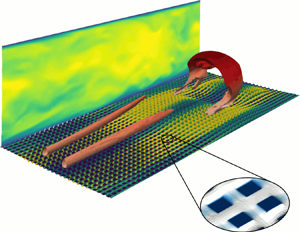
1. Introduction
Inspired from the leaves of the Nelumbo nucifera, the Lotus flower, researchers are currently investigating the physical mechanisms involved in highly water-repellent solid substrates such as superhydrophobic surfaces (SHS) (Barthlott et al. Reference Barthlott, Mail, Bhushan and Koch2017). The surface of Lotus leaves is composed of a hierarchical structure able to trap air pockets inside its micro- and nano-cavities, reducing the wetting capacity of water droplets falling on the leaves by reducing the area of direct contact of the liquid with the solid substrate. Thisprovides to the leaves their notable self-cleaning properties, since water droplets easily roll away from their surface (Schellenberger et al. Reference Schellenberger, Encinas, Vollmer and Butt2016) collecting solid impurities (Barthlott & Neinhuis Reference Barthlott and Neinhuis1997). Even when fully submerged in water, SHS may, in particular flow conditions, trap and retain gas bubbles within their micro-roughnesses (Cassie & Baxter Reference Cassie and Baxter1944). In these particular conditions, SHS have shown their potential in reducing the skin friction drag of an overlying flow, by providing a lubricating air layer (plastron) (Daniello, Waterhouse & Rothstein Reference Daniello, Waterhouse and Rothstein2009; Castagna, Mazellier & Kourta Reference Castagna, Mazellier and Kourta2018), whose macroscopic effect is similar to that of a slippery boundary (Rothstein Reference Rothstein2010).
The main barrier to many potential applications of SHS as a passive mean of drag reduction is the depletion of the lubricating gas layer. In fact, the amount of wall slip experimentally attainable is limited by the size of the micro-roughnesses, since larger air–water interfaces are more prone to wetting transition, as observed and theoretically predicted both in laminar (Ybert et al. Reference Ybert, Barentin, Cottin-Bizonne, Joseph and Bocquet2007) and turbulent (Seo, García-Mayoral & Mani Reference Seo, García-Mayoral and Mani2015) flows. When depletion of the gas bubbles occurs, the liquid fills the roughness elements (Wenzel Reference Wenzel1936), transforming the SHS into a wet, drag-increasing rough surface (Ling et al. Reference Ling, Srinivasan, Golovin, McKinley, Tuteja and Katz2016; Zhang, Yao & Hao Reference Zhang, Yao and Hao2016; Gose et al. Reference Gose, Golovin, Boban, Mabry, Tuteja, Perlin and Ceccio2018). For laminar overlying flows, the causes of plastron instability have been extensively studied (Wexler, Jacobi & Stone Reference Wexler, Jacobi and Stone2015; Patankar Reference Patankar2016). Only recently, Seo et al. (Reference Seo, García-Mayoral and Mani2015) and Seo, García-Mayoral & Mani (Reference Seo, García-Mayoral and Mani2017) have quantified the physical mechanism involved in the failure of the liquid–gas interfaces supporting fully developed turbulent flows. The ‘boundary map for stable superhydrophobic surface design’ proposed by Seo et al. (Reference Seo, García-Mayoral and Mani2017) suggests that using the maximum texture size ( $L_c^+$), ensuring wetting-stable conditions, the obtained reduction of the drag would be lower than
 $30\,\%$. This prediction is consistent with recent experimental observations (Bidkar et al. Reference Bidkar, Leblanc, Kulkarni, Bahadur, Ceccio and Perlin2014; Park, Sun & Kim Reference Park, Sun and Kim2014; Zhang et al. Reference Zhang, Tian, Yao, Hao and Jiang2015; Ling et al. Reference Ling, Srinivasan, Golovin, McKinley, Tuteja and Katz2016; Zhang et al. Reference Zhang, Yao and Hao2016; Gose et al. Reference Gose, Golovin, Boban, Mabry, Tuteja, Perlin and Ceccio2018), therefore providing a reliable threshold value of the micro-texture size for ensuring a drag reduction effect of SHS for turbulent flows. As a consequence, the typical size of a wetting-stable SHS roughness is up to two orders of magnitude smaller than the characteristic length of the overlying turbulent flow (Seo et al. Reference Seo, García-Mayoral and Mani2017). In these conditions, the slippery wall does not directly modify the overlying turbulent dynamics (Fairhall, Abderrahaman-Elena & García-Mayoral Reference Fairhall, Abderrahaman-Elena and García-Mayoral2018), and the mechanism for drag reduction is akin to that observed in flows over riblets (Luchini, Manzo & Pozzi Reference Luchini, Manzo and Pozzi1991).
Accurate numerical simulation of wetting transition, characterised by the gas–liquid–solid contact line dynamics, surface tension and liquid–gas diffusion, is an extremely complex task, requiring sophisticated and computationally demanding methods such as free-energy simulations (Lisi et al. Reference Lisi, Amabili, Meloni, Giacomello and Casciola2017). However, these methods are still not adapted for simulating macroscopic flows at high Reynolds number. To overcome this problem, researchers have proposed different, increasingly complex, models for describing the effect of the superhydrophobic surfaces on the overlying macroscopic flow, bearing in mind that simpler models have a considerably lower computational cost than more complex ones. In the following, we shortly introduce the most common models, in decreasing order of complexity. The first assumption that one can make to simplify the considered problem is that, in order to provide drag reduction, the lubricating plastron layer must be retained within the surface sculptures. Hence, one can consider the air–water interfaces as securely pinned to the roughness edges (Steinberger et al. Reference Steinberger, Cottin-Bizonne, Kleimann and Charlaix2007; Seo et al. Reference Seo, García-Mayoral and Mani2015), ensuring unconditionally wetting-stable conditions. Despite this hypothesis, numerically simulating the multi-scale physics of a two-phase flow over geometrically complex surfaces remains computationally challenging. Therefore, at the moment, such an approach has been used only in the case of low-Reynolds-number laminar flows (Li, Alame & Mahesh Reference Li, Alame and Mahesh2017; Alinovi & Bottaro Reference Alinovi and Bottaro2018; Bottaro Reference Bottaro2019).
To reach the turbulent regime at an affordable computational cost, Seo et al. (Reference Seo, García-Mayoral and Mani2017) have modelled the superhydrophobic surfaces as patterned slip and no-slip boundary conditions reproducing the spatial structure of the SHS texture. On the slippery regions, corresponding to the micro-cavities filled by gas pockets, the gas–liquid interface dynamics is taken into account using a linearised Young–Laplace equation, coupling the interface dynamics with that of the overlying turbulent flow. Simply speaking, this approach replaces the air–water surface with an equivalent hyperelastic compliant (Gad-El-Hak, Blackwelder & Riley Reference Gad-El-Hak, Blackwelder and Riley1984; Luhar, Sharma & McKeon Reference Luhar, Sharma and McKeon2015) slippery membrane. Using such a method, Seo et al. (Reference Seo, García-Mayoral and Mani2017) confirmed that the interface fluctuations are much smaller than the overlying flow coherent structures (Martell, Rothstein & Perot Reference Martell, Rothstein and Perot2010), and that the free-surface deformation does not alter the mean nor the fluctuations of the velocity profiles in turbulent statistics (notably, the displacement of the interface is of order  $1$ in the viscous length scale). Given the weakness of the interface displacements, a further approximation may be made, resulting in a simpler (computationally cheaper) model in which gas–liquid interfaces are assumed to be flat and the superhydrophobic surface is modelled as an alternation of no-slip/shear-free patterned patches (Martell et al. Reference Martell, Rothstein and Perot2010; Park, Park & Kim Reference Park, Park and Kim2013; Jelly, Jung & Zaki Reference Jelly, Jung and Zaki2014; Rastegari & Akhavan Reference Rastegari and Akhavan2015; Seo et al. Reference Seo, García-Mayoral and Mani2015, Reference Seo, García-Mayoral and Mani2017; Fairhall et al. Reference Fairhall, Abderrahaman-Elena and García-Mayoral2018), greatly reducing the complexity and the cost of numerical simulations (Seo et al. Reference Seo, García-Mayoral and Mani2017). An even simpler approach consists of using a macroscopic, spatially homogeneous Navier (Robin) slip boundary condition (Navier Reference Navier1823)
 \begin{equation} u_{s}=L^{(u)}_s\frac{\partial u}{\partial n},\quad v=0,\quad w_{s}=L^{(w)}_s\frac{\partial w}{\partial n}, \end{equation}
to model at the cheapest computational cost the streamwise, the wall-normal and the spanwise velocity components  $u,v,w$ over a superhydrophobic surface (Min & Kim Reference Min and Kim2004; Zampogna, Magnaudet & Bottaro Reference Zampogna, Magnaudet and Bottaro2018; Bottaro Reference Bottaro2019). In this case the average streamwise and spanwise velocities on the boundary,
 $u_s\ {\rm and}\ w_s$, called slip velocities, are both linked to the mean wall shear by a constant, the slip length
 $L_s$. In the particular case of isotropic SHS,
 $L^{(u)}_s=L^{(w)}_s=L_s$, as will be supposed in the present case. Seo & Mani (Reference Seo and Mani2016) have proven that, in the limit of small roughness size, the slip length model provides the same mean velocity profile and root-mean-square velocity fluctuations as those measured considering spatially heterogeneous slip–no-slip boundaries. Many recent studies have shown that these models provide almost equivalent results, both in laminar (Davis & Lauga Reference Davis and Lauga2010; Li et al. Reference Li, Alame and Mahesh2017) and in turbulent regimes, as long as some key physical constraints are satisfied (Seo & Mani Reference Seo and Mani2016; Seo et al. Reference Seo, García-Mayoral and Mani2017). However, the laminar–turbulent transitional regime remains, to the present day, mostly unexplored, except for the works by Min & Kim (Reference Min and Kim2005) and Picella, Robinet & Cherubini (Reference Picella, Robinet and Cherubini2019b), where only the slip length model was used. In particular, Picella et al. (Reference Picella, Robinet and Cherubini2019b) have shown that superhydrophobic walls modelled with a simple homogeneous slip length (HSL) model can affect or not transition in a channel flow, depending on the specific considered transition scenario. While being totally ineffective in delaying non-modal, uncontrolled transition dominated by streamwise velocity modulations (streaks) (Jacobs & Durbin Reference Jacobs and Durbin2001; Brandt et al. Reference Brandt, Cossu, Chomaz, Huerre and Henningson2003), homogeneously slippery walls have proven to effectively delay or even inhibit the onset of turbulence in scenarios characterised by the presence of near-wall structures, such as the K-type transition process (Nishioka, Iid A & Ichikawa Reference Nishioka, Iid A and Ichikawa1975; Kleiser & Zang Reference Kleiser and Zang1991; Schlatter, Stolz & Kleiser Reference Schlatter, Stolz and Kleiser2006). Reducing the wall shear, the slippery boundary interferes with the development of coherent structures usually occurring during this specific transition scenario, altering the vortex stretching–tilting processes that produces
 $\Lambda$ and hairpin vortices (Malm, Schlatter & Sandham Reference Malm, Schlatter and Sandham2011; Sayadi, Hamman & Moin Reference Sayadi, Hamman and Moin2013). Depending on the considered value of the slip length, SHS inhibit the sweep–ejection processes sustaining hairpin vortices, drastically retarding or even avoiding their breakdown to turbulence. Although the K-type process, representative of modal transition, is strongly influenced by the introduction of a slippery boundary, this is not a general result. Picella et al. (Reference Picella, Robinet and Cherubini2019b) have shown that, when transition is triggered by a broadband noisy forcing (Picella et al. Reference Picella, Bucci, Cherubini and Robinet2019a), SHS modelled with a simple homogeneous partial slip condition weakly affect the transition process. However, it is still unclear if and how more physically accurate models, including spatial heterogeneity and/or interface dynamics, may affect the laminar–turbulent transition process. Avoiding or delaying transition to turbulence in fact may be of huge practical interest for applications requiring the transport of flows in channels or pipes, where turbulence is the primary cause of friction losses. In fact, transition from laminar to turbulent conditions induces a consistent drag increase in flows over bounding surfaces. Although superhydrophobic surfaces are currently used to reduce turbulence intensities in fully turbulent flows, they have not yet been tested for altogether avoiding turbulence, by keeping the flow laminar even for values of the Reynolds number for which transition is usually observed. Superhydrophobic surfaces that succeed at hindering the laminar–turbulent transition process may potentially lead to an even stronger reduction of friction losses with respect to those working on turbulent flows (see Picella et al. Reference Picella, Robinet and Cherubini2019b, where a
 $50\,\%$ reduction of the drag was reported by avoiding turbulent transition), which can lead to a huge energy saving in the flow transport process. The aim of this work is thus to verify the robustness of the behaviour of transitional flows on SHS with respect to different SHS models, similarly to what has already been done in the literature for both laminar (Ou, Perot & Rothstein Reference Ou, Perot and Rothstein2004) and turbulent (Seo & Mani Reference Seo and Mani2016; Seo et al. Reference Seo, García-Mayoral and Mani2017) regimes.
Towards this aim, in this work we investigate the influence of the SHS modelling on different laminar–turbulent transition processes, by means of global linear stability analysis and time resolved direct numerical simulations (DNS). Modal and non-modal transition scenarios are considered for a channel flow at subcritical flow conditions. For modal transition scenarios, we consider the K-type process (Klebanoff, Tidstrom & Sargent Reference Klebanoff, Tidstrom and Sargent1962; Sandham & Kleiser Reference Sandham and Kleiser1992; Kachanov Reference Kachanov1994; Sayadi et al. Reference Sayadi, Hamman and Moin2013), which has been already studied in the literature using the simple slip length model. As a prototype of non-modal transition, we initialise the flow with the F-type (Picella et al. Reference Picella, Bucci, Cherubini and Robinet2019a) method, where a stochastic volume forcing reproducing environmental noisy disturbances is used to trigger transition. In both cases, we have considered SHS constituted of a regular pattern of square posts due to their relevance in studying arbitrary disposed, sprayed-like coatings (Seo & Mani Reference Seo and Mani2018) and at the same time to allow a direct comparison with literature simulations in the turbulent regime (Seo & Mani Reference Seo and Mani2016; Seo et al. Reference Seo, García-Mayoral and Mani2017). Moreover, considering spatially isotropic SHS composed of square post allows us to simplify the modelling process, when using spatially homogeneous (Min & Kim Reference Min and Kim2004) or heterogeneous equivalent boundary conditions (Seo et al. Reference Seo, García-Mayoral and Mani2017). The roughness size of the SHS has been selected based on the design principles proposed by Seo et al. (Reference Seo, García-Mayoral and Mani2017), namely, sufficiently small to ensure wetting stability while providing the highest possible slip. The investigation in this work shows that when transition is triggered by near-wall disturbances (such as in the K-type scenario), considering the air–water interface deformation is crucial for accurately simulating flow transition. In fact, the interface displacement introduces a non-zero wall-normal velocity at the wall boundaries which, despite being small, promotes ejection mechanisms which advance transition with respect to the results of the slip length model.
The paper is organised as follows. In § 2 we present the governing equations and the methods used to implement the different models of SHS, and we discuss the main characteristic lengths and dimensionless parameters of the problem. In § 3 we show, using local and global stability analysis, how the dynamics of infinitesimal perturbations is influenced by differently modelled SHS. Section 4 reports the results of direct numerical simulations of laminar–turbulent K-type transition, for the different considered SHS models. In particular we show that, taking into account the gas–liquid interface displacement strongly affects the transition process. Section 5 then discusses the influence of SHS on non-modal F-type transition, showing that this transition scenario is almost insensitive to the different surface models. A direct comparison of the influence of the interface displacement on the two types of transition is discussed in § 6. A final discussion and conclusions are given in § 7.
2. Problem formulation
The channel flow configuration is chosen to study how laminar–turbulent transition could be controlled using superhydrophobic walls capable of entrapping a gas-lubricating layer. Assuming that air–water interfaces are kept pinned to the roughness surfaces, as sketched in figure 1, the influence of superhydrophobic surfaces can be modelled with an equivalent boundary condition for the overlying, incompressible Newtonian flow, governed by the non-dimensional Navier–Stokes equations
 \begin{gather} \frac{\partial \boldsymbol U}{\partial t} = -({\boldsymbol U} \,{\boldsymbol \cdot}\, {\boldsymbol \nabla}) {\boldsymbol U} -{\boldsymbol \nabla} P +\frac{1}{Re}\nabla^2 {\boldsymbol U} + {\boldsymbol f}, \end{gather}
 \begin{gather}{\boldsymbol \nabla} \,{\boldsymbol \cdot}\, {\boldsymbol U} = 0, \end{gather}
where  ${\boldsymbol U}=(U({\boldsymbol x},t),V({\boldsymbol x},t),W({\boldsymbol x},t))^T$ is the velocity field,
 $P({\boldsymbol x},t)$ is the pressure and
 ${\boldsymbol f}$ the forcing field, all being non-dimensional quantities defined with respect to the centreline velocity
 $U$ and the half-height of the channel
 $H$. The relevant time scale is thus
 $H/U$. The Reynolds number is defined as
 $Re = {U H} / \nu$,
 $\nu$ the kinematic viscosity of the fluid. The reference frame
 ${\boldsymbol x}=(x,y,z)^T$ is chosen such that
 $x$ is the streamwise,
 $y$ the wall-normal and
 $z$ the spanwise direction. The micro-roughnesses consist of square post of width
 $W$, placed at a distance
 $L$ between them. The water–gas interface is maintained within the edges of the roughness elements by capillary forces, characterised by the surface tension
 $\sigma$, dependent on the gas–liquid physical properties. The effect of the water–gas interface on the overlying flow has been modelled in different ways (as detailed in § 2.1, and sketched in figure 2), leading to three different boundary conditions which have been implemented within Nek5000 (Fischer, Lottes & Kerkemeier Reference Fischer, Lottes and Kerkemeier2008), a spectral element method flow solver. Periodicity is assumed in the streamwise and spanwise directions.
Sketch of a channel flow with superhydrophobic surfaces at the walls, depicting the length-scale gap between the overlying laminar–turbulent macroscopic flow whose coherent structures may reach sizes of order  $H$ and the near-wall, capillary-driven microscopic free-surface dynamics having characteristic length
 $L$.

Channel flow over a smooth, flat wall (a) and over superhydrophobic surfaces modelled with increasingly complex boundary conditions (b–d).

2.1. Modelling superhydrophobic surfaces
The effect of the SHS on the overlying flow has been at first modelled as a spatially homogeneous Navier boundary condition on the surface, as in (1.1a–c). This approach, based on the homogenisation theory (Zampogna et al. Reference Zampogna, Magnaudet and Bottaro2018), provides a computationally inexpensive method to describe the influence of gas-lubricated substrates. In fact, simulations with Navier boundary conditions have proven to predict well the experimental results in both the laminar (Rothstein Reference Rothstein2010) and turbulent regimes (Ling et al. Reference Ling, Srinivasan, Golovin, McKinley, Tuteja and Katz2016; Seo & Mani Reference Seo and Mani2016), provided that the value of the slip length  $L_s$ is well evaluated (Seo et al. Reference Seo, García-Mayoral and Mani2015). The choice of using SHS made out of square posts allows the use of a single, constant slip length, in contrast with what would occur when dealing with anisotropic SHS patterns (Pralits, Alinovi & Bottaro Reference Pralits, Alinovi and Bottaro2017) or considering shear-dependent slip lengths (Aghdam & Ricco Reference Aghdam and Ricco2016). In the remainder of this work we will refer to this approach as spatially homogeneous slip length (HSL).
The second model used here considers the upper surface of every square post as a solid boundary, on which a no-slip condition is applied. Between the posts, in the micro-cavities in which the gas is trapped, the overall effect of the gas–water interface is treated as a shear-free boundary condition. The underlying assumption is that the gas–water interface remains perfectly flat while providing a shear-free boundary, a standard assumption used in the literature for DNS of turbulent flows on SHS (Martell, Perot & Rothstein Reference Martell, Perot and Rothstein2009; Jelly et al. Reference Jelly, Jung and Zaki2014; Park et al. Reference Park, Sun and Kim2014; Lee, Choi & Kim Reference Lee, Choi and Kim2016). The implementation of such method is straightforward, but it should be considered that discretising micro-roughnesses with texture size sufficiently small to ensure wetting-stable conditions requires numerical grids which are one order of magnitude finer than those used in the HSL case (as an example, one can compare cases P06 and HP06 in Seo & Mani Reference Seo and Mani2016). In the remainder of this work we will refer to this approach as slip/no slip (SNS).
Similarly to the previous, the third model relies on the discretisation of the single square post, but in this last case the gas–water interface is not assumed to be flat, its dynamical deformation being taken into account. Following the work of Seo et al. (Reference Seo, García-Mayoral and Mani2017), we consider an ideal shear-free boundary condition on the air–water interface (Schönecker, Baier & Hardt Reference Schönecker, Baier and Hardt2014), that neglects the plastron viscosity (Schönecker et al. Reference Schönecker, Baier and Hardt2014), whilst ensuring that the interface remains pinned to the post edges (Steinberger et al. Reference Steinberger, Cottin-Bizonne, Kleimann and Charlaix2007; Teo & Khoo Reference Teo and Khoo2010; Seo et al. Reference Seo, García-Mayoral and Mani2015). Under these assumptions the free-surface deformation  $\eta$ is linked to the liquid pressure at the interface via a linearised Young–Laplace equation,
 \begin{equation} \nabla^2 \eta \approx \frac{P_{liquid} - P_{gas}}{\sigma}, \end{equation}
where  $\sigma$ is the surface tension and, assuming
 $P_{gas}$ to be uniform within all the lubricating gas layer, the plastron's mass conservation yields
 \begin{equation} \int\int \eta(x,z,t) \, \textrm{d} x \, \textrm{d} z = 0 . \end{equation}
Thus, we solve (2.1) over a time-dependent, deforming boundary, constituting a two-way coupled fluid–structure interaction problem. While this approach still neglects both the motion of the lubricating gas (Alamé & Mahesh Reference Alamé and Mahesh2019) and the possible dynamics of the triple point (Gose et al. Reference Gose, Golovin, Boban, Mabry, Tuteja, Perlin and Ceccio2018), to the authors’ knowledge it represents the only method capable of accounting for the SHS liquid–gas microscopic interfaces, while sustaining a macroscopic flow undergoing turbulent transition (Seo et al. Reference Seo, García-Mayoral and Mani2017).
In the present study we make use of an arbitrary Lagrangian–Eulerian (ALE) description (Ramaswamy & Kawahara Reference Ramaswamy and Kawahara1987) to simulate the free-surface deformation, taking advantage of the implementation of Lee-Wing & Patera (Reference Lee-Wing and Patera1990), natively coded and validated within Nek5000 (Lee-Wing Reference Lee-Wing1989). This approach provides an accurate and numerically efficient description of the free-surface dynamics while ensuring the kinematic condition
 \begin{equation} {\boldsymbol w} \, {\boldsymbol \cdot}\, \hat{{\boldsymbol n}}|_{\eta} = {\boldsymbol U} \,{\boldsymbol \cdot}\, \hat{{\boldsymbol n}}|_{\eta}, \end{equation}
where  ${\boldsymbol w}$ is the mesh velocity and
 $\hat {{\boldsymbol n}}$ is the unit vector normal to the interface
 $\eta (x,z,t)$ (see figure 2d). Provided that the mesh velocity at the wall is
 ${\boldsymbol w}|_{wall}=\dot {\eta }$, this moving boundary (MVB) model allows for non-zero wall-normal velocity components over the interface. Although the resulting wall-normal velocity at the boundary is negligible in fully turbulent flows over realistic SHS (Seo et al. Reference Seo, García-Mayoral and Mani2017), we will show that it can strongly affect the processes occurring during the transitional phase. As a further remark we would like to highlight that, owing to the small values of
 $\eta$ compatible with wetting-stable conditions, the wall-normal velocity induced by the interface deformation will assume the form
 \begin{equation} {\boldsymbol V}(x,y=\eta,z,t)=\frac{D \eta}{D t} = \frac{\partial \eta}{\partial t} + U \frac{\partial \eta}{\partial x} + W \frac{\partial \eta}{\partial z}, \end{equation}
as found by Seo et al. (Reference Seo, García-Mayoral and Mani2017) by linearising the boundary condition for  $V$ at
 $y=\pm 1$. Whereas Neumann shear-free boundary conditions are used for both streamwise and spanwise velocities on top of the gas–liquid interfaces, in both MVB and SNS cases. The three different models for the simulation of SHS are sketched in figure 2, together with the smooth-wall no-slip boundary condition providing the standard plane Poiseuille flow (PPF).
2.2. Simulation parameters
In this work we study if and how modal and non-modal transition (Schmid & Henningson Reference Schmid and Henningson2001) in channel flows can be controlled or delayed using superhydrophobic surfaces. As detailed in § 4, concerning the modal scenario we use K-type transition (Kachanov Reference Kachanov1994), whereas for non-modal ones we choose the F-type approach (Picella et al. Reference Picella, Bucci, Cherubini and Robinet2019a). Following many works in the literature (Kim, Moin & Moser Reference Kim, Moin and Moser1987), numerical simulations are performed in a streamwise- and spanwise-periodic channel flow. A computational box of size  $2{\rm \pi} /\alpha \times 2H \times 2{\rm \pi} /\beta$ is used, where
 $\alpha$ and
 $\beta$ are the lowest streamwise and spanwise wavenumbers allowed in the computational domain. As in many works in the literature, in performing DNS of transitional channel flows (Zang & Krist Reference Zang and Krist1989; Gilbert & Kleiser Reference Gilbert and Kleiser1990; Schlatter Reference Schlatter2005) we set
 $(\alpha ,\beta )=(1.12,2.10)$ and a constant flow rate, corresponding to a laminar Reynolds number of
 $Re=5000$. The fully developed turbulent flow is characterised by the friction Reynolds number
 $Re_\tau =\delta / \delta _\nu =u_\tau \delta / \nu$, measuring the ratio between the external scales (
 $\delta \equiv H$ in channel flow) and the viscous unit length
 $\delta _\nu = \nu / u_\tau$;
 $Re_\tau$ here is computed a posteriori, using different formulations depending on the particular SHS model employed. Under the flat-interface approximation (i.e. in the HSL and SNS cases), the friction Reynolds number is defined as
 \begin{equation} Re_\tau=\sqrt{Re \left| \frac{\partial \langle U({\boldsymbol x},t)\rangle }{\partial y} \right|_{y=\pm1}}, \end{equation}
where  $\langle \bullet \rangle$ represents the spatial average on the wall-parallel planes
 $x-z$ at a given time
 $t$. Following the notation used in the present work, the Reynolds decomposition reads as
 \begin{equation} {\boldsymbol{U}} = \langle {\boldsymbol{U}} \rangle + {\boldsymbol{U}}^{\prime} = \langle {\boldsymbol{U}} (t) \rangle _{x,z} + {\boldsymbol{U}}^{\prime}. \end{equation}
When describing the statistically converged fully turbulent phases, the  $\langle \bullet \rangle$ notation will be used to identify quantities averaged on the wall-parallel planes
 $x-z$, as well as over time
 $t$.
As in the case of flows over compliant surfaces (Rosti & Brandt Reference Rosti and Brandt2017), in the MVB case the definition of  $Re_\tau$ must be modified to take into account the shear stresses which are non-zero at the moving interface. Following Breugem, Boersma & Uittenbogaard (Reference Breugem, Boersma and Uittenbogaard2006), the friction Reynolds number computed over a moving surface becomes
 \begin{equation} Re_\tau=\sqrt{Re \left| \frac{\partial \langle U({\boldsymbol x},t)\rangle }{\partial y} \right|_{y=\pm1} - \left| \langle U^{\prime} V^{\prime} \rangle \right|_{y=\pm1}}, \end{equation}
where  $\langle U^\prime V^\prime \rangle$ is the off-diagonal component of the Reynolds stress tensor, evaluated on the spatially heterogeneous deformed SHS surface. This additional term can potentially account for up to
 $10\,\%$ of the
 $Re_\tau$ value, when the SHS is modelled using the MVB approach. This can possibly lead to a difference of the averaged
 $Re_\tau$ value achieved in fully turbulent conditions in the MVB case with respect to the other cases.
All the models proposed here consider the gas as trapped inside the micro-roughness, with no possibility of escaping. Therefore, we should ensure that, under the chosen flow conditions, the gas–water interfaces would remain indeed wetting stable (Seo et al. Reference Seo, García-Mayoral and Mani2017). A key dimensionless parameter for wetting transition is the size of the texture in viscous units  $L^+=L/\delta _\nu$. Experiments have demonstrated that SHS having
 $L^+ < 0.5-10$ are capable of maintaining wetting-stable conditions while sustaining a fully developed turbulent flow (Daniello et al. Reference Daniello, Waterhouse and Rothstein2009; Woolford et al. Reference Woolford, Prince, Maynes and Webb2009; Park et al. Reference Park, Sun and Kim2014; Li et al. Reference Li, Alame and Mahesh2017; Gose et al. Reference Gose, Golovin, Boban, Mabry, Tuteja, Perlin and Ceccio2018), whereas larger surface texture may not be capable of remaining wetting stable under certain flow conditions (Zhang et al. Reference Zhang, Yao and Hao2016). This point must be considered when choosing appropriate values of the texture size (in the SNS and MVB cases) and of the slip length, which cannot be set larger than the values actually observed in experiments. In previous numerical investigations of laminar–turbulent transition over superhydrophobic surfaces (Min & Kim Reference Min and Kim2005; Picella et al. Reference Picella, Robinet and Cherubini2019b), the largest slip length considered is
 $L_s=0.02$, which we consider as a benchmark value. In order to compare the influence of surface modelling on the transition process, we must determine the surface texture size required in the SNS and MVB cases to provide the same amount of slip of the HSL case. Towards this aim, we use the universal slip length representation for turbulent flows over SHS, (i.e. (15) in the work by Seo et al. Reference Seo, García-Mayoral and Mani2015)
 \begin{equation} L^+ = \frac{L_s^+}{C_b}+0.328(L_s^+\sqrt{\phi_s})^3, \end{equation}
where the coefficient  $C_b = (0.325 / \sqrt {\phi _s})-0.44$,
 $\phi _s$ is the liquid–solid/liquid–gas area ratio of the texture pattern and
 $L_s^+$ is the slip length in viscous units.
Setting a fixed laminar Reynolds number and reaching the turbulent flow regime keeping a constant flow rate, the friction Reynolds number will decrease due to the drag reduction effect of the superhydrophobic surfaces. In previous studies of transitional flows over SHS modelled with a homogeneous slip length (Picella et al. Reference Picella, Robinet and Cherubini2019b), setting  $L_s=0.02$ resulted in
 $Re_\tau \approx 190$, therefore
 $L_s^+=Re_\tau L_s\approx 3.8$. To obtain the same equivalent homogeneous slip length
 $L_s^+=3.8$ using the SNS and MVB models, we first fix the solid fraction to the value
 $\phi _s=0.25$. Under this hypothesis, using (2.10) we obtain
 $L^+ \approx 20$, equivalent to a texture size
 $L\approx 0.105$. Despite the texture size used in the present study is larger than the upper limit proposed by Seo & Mani (Reference Seo and Mani2016) for the perfect equivalency of HSL and SNS models (
 $L^+\leq 10$), we show in appendix B that the chosen value of
 $L$ is still sufficiently small to guarantee the same turbulent statistics when using texture-resolved surfaces (SNS) or an equivalent spatially homogeneous slippery boundary (HSL). It follows that accounting for superhydrophobic surfaces using spatially heterogeneous SNS and MVB models requires spatial discretisation of
 $(2{\rm \pi} / \alpha ) / L \approx 53$ and
 $(2 {\rm \pi}/ \beta ) / L \approx 28$ posts in the streamwise and spanwise directions, respectively. Each liquid–solid/liquid–gas interface has to be discretised with a single spectral element owing to the numerical constraints of our numerical code. Thus, our computational domain will be composed of 106 elements in the streamwise direction and 56 in the spanwise one in order to simulate isotropic square posts. Choosing a spectral order of 8, each texture element is discretised with 16 grid points per direction which, according to a recent study (Fairhall & García-Mayoral Reference Fairhall and García-Mayoral2018), allows an accurate computation of fully turbulent flows, being therefore sufficient also for the study of transitional ones. Obviously, the use of the Navier boundary condition as in the HSL model greatly reduces the computational cost of the simulations. In table 1 we report the numerical parameters employed during the present study, depending on the considered surface model. In the case of homogeneous surface modelling, we have used as a reference the numerical parameters employed in Picella et al. (Reference Picella, Bucci, Cherubini and Robinet2019a).
Simulation parameters for the DNS of channel flow at  $Re_\tau \approx 200$ using different SHS models.
 ${E}_{x,y,z},{N}_{x,y,z}$ indicate the number of finite element and total grid points in each spatial direction, respectively;
 $\langle {\rm \Delta} x^+\rangle ,\langle {\rm \Delta} z^+\rangle$ indicate the averaged grid size scaled in friction units in the streamwise and spanwise directions, respectively, and
 ${\rm \Delta} y^+|_{wall,centre}$ indicate the grid size in the wall-normal direction at the wall and at the centre of the channel scaled in friction units.

When using MVB modelling of SHS, we have to set the surface tension  $\sigma$ of the gas–liquid interface. In the present study we assume an air-lubricated turbulent water channel at a
 $20\,^\circ$C, having
 $\sigma =0.072$ N m
 $^{-1}$,
 $\rho \approx 10^3\ \textrm {N}\,\textrm {s}^2\,\textrm {m}^{-4}$ and
 $\nu \approx 10^{-5}\ \textrm {m}^2\,\textrm {s}^{-1}$. Since at
 $Re_\tau =190$ we have
 $u_\tau \approx 0.038$ m s
 $^{-1}$, and considering that
 $u_\tau \delta _{\nu } = \nu$, in the considered flow conditions we find a Weber number
 $We^+=\rho u_\tau ^2 \delta _\nu / \sigma =\rho u_\tau \nu / \sigma \approx 5 \times 10^{-4}$. These values of
 $We^+$ and
 $L^+$ are comparable with those measured experimentally in wetting-stable conditions by Seo et al. (Reference Seo, García-Mayoral and Mani2017), while choosing larger values of these parameters may lead to a destabilisation of the liquid–gas interface.
3. Influence of surface modelling on linear stability
In this section we study if and how flow stability is modified by the use of different surface models of the SHS. We consider small-amplitude disturbances  ${\boldsymbol q}({\boldsymbol x},t)=({\boldsymbol u},p)^T$ of the base flow
 ${\boldsymbol Q}_b({\boldsymbol x})=({\boldsymbol U}_b, P)^T$, which is a steady solution of the Navier–Stokes equations (2.1), so that
 ${Q}({\boldsymbol x},t)={\boldsymbol Q}_b({\boldsymbol x}) + {\boldsymbol q}({\boldsymbol x},t)$. The dynamics of such perturbations is governed by the linearised Navier–Stokes equations, which once projected on a divergence-free vector space can be compactly written as
 \begin{equation} \frac{\partial {\boldsymbol u}}{\partial t} = {\boldsymbol J}{\boldsymbol u}. \end{equation}
Provided that (3.1) is a linear dynamical system autonomous in time, we can expand the perturbation in normal modes, such that  ${\boldsymbol u}({\boldsymbol x},t) = \sum _{k=1}^\infty \hat {{\boldsymbol u}}_k({\boldsymbol x}) \, \textrm {e}^{\lambda _k t}$. Injecting this expansion into (3.1) yields an eigenvalue problem
 \begin{equation} \lambda_k \hat{{\boldsymbol u}_k} = {\boldsymbol J} \hat{{\boldsymbol u}_k}, \end{equation}
where  $\lambda _k=\sigma _k + \textrm {i} \omega _k$ is the eigenvalue and
 $\hat {{\boldsymbol u}_k}$ its associated eigenvector;
 $\sigma _k$ and
 $\omega _k$ represent, respectively, the growth rate and the pulsation of each eigenmode. Beyond a critical value of the Reynolds number (
 $Re_c$) one eigenvalue of
 ${\boldsymbol J}$ reaches a growth rate
 $\sigma _k > 0$, thus the base flow becomes linearly unstable.
Min & Kim (Reference Min and Kim2005) were the first to determine the influence of SHS on the stability of a pressure driven channel flow using an HSL model. Under this assumption the base flow is dependent only on the wall-normal direction (Philip Reference Philip1972)
 \begin{equation} U_b(y)_{HSL}= \frac{2 L_s + 1 -y^2}{3 L_s + 1}, \end{equation}
as in the case of the plane Poiseuille flow. Therefore, the eigenvectors can be further expanded as
 \begin{equation} {\boldsymbol u}({\boldsymbol x},t) = \sum_{k=1}^\infty \hat{{\boldsymbol u}}_k (y) \, \textrm{e}^{\lambda_k t} \exp({\textrm{i} (\alpha x + \beta z)})+ \textrm{c.c.}, \end{equation}
where  $\textrm {c.c.}$ is the complex conjugate and
 $\alpha$ and
 $\beta$ represent the streamwise and spanwise wavenumbers, respectively, leading to computationally inexpensive one-dimensional local stability analysis (Orszag Reference Orszag1971). Min & Kim (Reference Min and Kim2005) have found that slippery surfaces stabilise the Tollmien–Schlichting waves (TS) while decreasing the wall shear
 $\partial U / \partial y$. As a result, the critical Reynolds number
 $Re_c$ increases with the slip length
 $L_s$ since
 $\partial U / \partial y = -2 y / (3 L_s +1)$.
In the following, we investigate if and how taking into account the spatial heterogeneity of the SHS affects these results. Depending on the micro-structure of the SHS, the base flow can be homogeneous only in one of the wall-parallel directions, or in none of them, invalidating the assumption (3.4) and requiring an increasingly complex framework to tackle the linear stability analysis problem. While in the case of streamwise ridges (Alinovi & Bottaro Reference Alinovi and Bottaro2018) two-dimensional local stability analysis can be appropriate (Yu, Teo & Khoo Reference Yu, Teo and Khoo2016), a SHS consisting of isotropic square posts provides a non-homogeneous base flow in both wall-parallel directions, therefore requiring the use of fully three-dimensional global stability analysis (Theofilis & Colonius Reference Theofilis and Colonius2003; Picella et al. Reference Picella, Loiseau, Lusseyran, Robinet, Cherubini and Pastur2018). In the latter case, for obtaining the three-dimensional base flow, we have run a DNS with superhydrophobic surfaces modelled using the SNS/MVB approaches, initialising the base flow with the homogeneous velocity profile in (3.3). When convergence to a steady state is reached (up to a residual lower than  $10^{-8}$) we obtain a three-dimensional base flow
 ${\boldsymbol U}_b({\boldsymbol x})=(U_b({\boldsymbol x}),V_b({\boldsymbol x}),W_b({\boldsymbol x}))$. We have also verified a posteriori that using the texture size
 $L$ computed from (2.10) results into an averaged slip velocity at the wall equivalent to that obtained using (3.3), namely
 $u_s=\langle u\rangle _{wall} = 2 L_s / (3 L_s + 1)$. Once the three-dimensional base flow is computed, we investigate the asymptotic stability of perturbations superposed on it. Due to the large number of degrees of freedom involved (
 $N_x \times N_y \times N_z \times 4 \rightarrow \mathcal {O} ( 3 \times 10^{8} )$), it appears clear that using direct methods (i.e. Schur or generalized Shur decompositions such as QR and QZ algorithms) to solve the eigenproblem (3.2) is hardly possible at the moment. Thus, we use a time-stepper formulation to find the leading eigenpairs of (3.1), based on the iterative Arnoldi algorithm (Arnoldi Reference Arnoldi1951) as described by Loiseau et al. (Reference Loiseau, Robinet, Cherubini and Leriche2014). Using a Krylov subspace of dimension
 $K=250$, we are able to compute the Tollmien–Schlichting waves over a spatially alternating slip–no-slip (SNS) modelled superhydrophobic surface. Figure 3(a) depicts the eigenspectra obtained using HSL and SNS models. With the HSL model, the base flow is parallel in both streamwise and spanwise directions, allowing the use of a one-dimensional local stability framework (Schmid & Henningson Reference Schmid and Henningson2001) for computing of the eigenmodes. This eigenvalue problem (3.2) has been solved for
 $\alpha =1.12, \beta =0.00$,
 $L_s=0.02$ in the HSL case. As predicted by Min & Kim (Reference Min and Kim2005), we find that the most unstable mode on a channel flow with slippery walls is a two-dimensional TS wave. Virtually the same TS wave has been obtained using the SNS model, despite the radically different stability framework and surface model employed. While in the SNS case a fully three-dimensional global stability analysis (Loiseau et al. Reference Loiseau, Robinet, Cherubini and Leriche2014) is required, the most unstable eigenvalue perfectly matches that computed for the HSL case (see figure 3a). Averaging the associated three-dimensional eigenvector along the wall-parallel planes we obtain an equivalent one-dimensional velocity profile, indicated as
 $\textrm {SNS}_{avg}$ in figure 3(b), which matches very well that computed using the HSL model. In fact, the characteristic length of the surface roughnesses is much smaller than that of the TS waves, not interfering much with their structure. Moreover, given the small value of
 $L$ chosen, the spatial heterogeneity in the wall-parallel planes rapidly fades away approaching the channel centre. For a more quantitative analysis we have defined the difference
 ${\boldsymbol U}_d({\boldsymbol x})$ of the three-dimensional base flow obtained in the SNS case and the one-dimensional steady flow recovered using the HSL approach
 \begin{equation} {\boldsymbol U}_{d}({\boldsymbol x}) = {\boldsymbol U}_b({\boldsymbol x})_{SNS} - (U_b(y)_{HSL},0,0)^{\rm T}, \end{equation}
where the last term is the one-dimensional velocity profile obtained using (3.3);  ${\boldsymbol U}_{d}$ constitutes a measure of the spatial heterogeneity of the base flow, similarly to thestreaks amplitude
 $A_s$ defined by Brandt et al. (Reference Brandt, Cossu, Chomaz, Huerre and Henningson2003) which provides a measure of the intensity of streamwise streaks occurring during transition (Andersson, Berggren & Henningson Reference Andersson, Berggren and Henningson1999). In order to get a one-dimensional profile deformation, we compute the average of
 $U_d$ along the wall-parallel directions, whose normalised profile is plotted in figure 4. One can notice how the base flow deformation is attenuated by almost
 $99\,\%$ from
 $y> -0.96$ (or equivalently,
 $y<0.96$). Whereas, the wall-normal location of the maximum amplitude of the most unstable TS wave is located at
 $\approx 0.875$ (indicated with a black dashed line in figures 3b and 4b), where the influence of the three-dimensionality of the flow is very weak. This explains how linear stability analysis computed with a one-dimensional local analysis on a base flow profile provides virtually the same result of a fully global stability analysis on a three-dimensional base flow. In figure 4, we also show the velocity profiles of the TS three-dimensional eigenvector taken at the
 $x-z$ location at which they reach their maximum (
 $\textrm {SNS}_{max}$) and minimum (
 $\textrm {SNS}_{min}$) amplitudes at the wall. These profiles show that the influence of the heterogeneous boundary conditions close to the wall is not negligible. However, the effect of spatial heterogeneity on the base flow rapidly fades when departing from the wall, as indicated by the
 $U_d$ profile. Let us consider now the influence of the air–water interface dynamics. The resulting base flow, obtained as converged steady solution of the Navier–Stokes equations with MVB approach at the boundaries, is indistinguishable from that computed for the SNS case. While in experiments the mass of the gas trapped within the surface pattern remains constant (unless wetting transition is occurring) the MVB model assumes that plastron volume is constant (see (2.4)). This, together with the fact that we initialise our base flow computation by setting the initial deformation to zero, say
 $\eta (x,z,t=0)=0$, results into a maximum free-surface deformation
 $\eta _{max}\approx 5 \times 10^{-5}$ which is two orders of magnitude smaller than the surface texture length scale
 $L$, therefore compatible with the linearised model described in (2.3), as shown by Seo et al. (Reference Seo, García-Mayoral and Mani2017).
(a) Eigenspectra of the linearised Navier–Stokes operator for a channel flow with superhydrophobic surfaces at  $Re=5000$, obtained with one-dimensional stability analysis for the HSL approximation, and with three-dimensional global stability analysis in the SNS case. (b) Norm of the streamwise component associated with the most unstable eigenvalue of the spectrum, where the mode obtained using SNS modelling has been averaged in the wall-parallel directions for the purpose of comparison to the HSL case.

(a) Iso-surfaces of the streamwise velocity of the least stable mode, computed in a channel with SNS modelled superhydrophobic surfaces. The quasi-two-dimensional Tollmien–Schlichting-like waves are obtained using a global stability framework. (b) Measures of the leading unstable eigenvector computed for HSL and SNS modelled superhydrophobic surfaces: velocity profiles of maximum and minimum amplitudes at the wall,  $\textrm {SNS}_{max}$ and
 $\textrm {SNS}_{min}$ and
 $x-z$ averaged one,
 $\textrm {SNS}_{avg}$, together with the normalised value of the base flow deformation
 $U_d$ introduced in (3.5).

Since interface dynamics is not implemented in the global stability analysis numerical code used for the SNS configuration, we use a continuation method (Theofilis & Colonius Reference Theofilis and Colonius2003) to get three-dimensional eigenfunctions starting from their respective local counterparts. The idea consists of injecting the eigenfunctions computed with the local stability analysis as initial condition for a DNS with MVB modelled superhydrophobic surfaces. As shown in figure 5, after a short transient, the local eigenmode used as initial condition adapts to the imposed spatially heterogeneous, deformable boundary condition. Despite the obtained global TS eigenfunctions being characterised by a non-trivial interface dynamics at the wall due to the coupling with the flow, their frequency and growth rate match almost perfectly those calculated using the fully global linear stability analysis tool in the SNS case. This behaviour is probably due to the fact that the length scale of the spatial heterogeneity ( $L$) is small compared to the channel size
 $H$. Under this assumption the continuation method allows an accurate estimation of the three-dimensional eigenvectors of (3.1) over SNS and MVB boundaries starting from those computed with one-dimensional local stability analysis in the HSL case. Thus, we have shown here that linear stability does not appear to be affected by the different methods used to model the SHS, provided that the texture size is sufficiently small to avoid any interaction with the macroscopic TS-like wave. This extends the observations made by Seo & Mani (Reference Seo and Mani2016) in the turbulent regime to the linear stability framework.
Time evolution of normalised wall-normal velocity extracted at  $(x,y,z)=(0,0.5,0)$ from three different DNS using the HSL (A), SNS (B) and MVB (C) approaches for modelling the superhydrophobic surfaces. The simulations have been initialised by adding on top of the respective base flows, the two-dimensional TS wave with
 $k_x=1.12,k_z=0$ computed by means of one-dimensional local stability analysis.

4. Modal transition
We now investigate the influence of the different models of the SHS on the nonlinear stages of the laminar–turbulent transition process. Concerning the modal transition scenarios, the K-type one (Klebanoff et al. Reference Klebanoff, Tidstrom and Sargent1962) has been chosen as first benchmark for the present study since it has been found to be very sensitive to the use of slippery boundary conditions in the recent work by Picella et al. (Reference Picella, Robinet and Cherubini2019b). K-type transition is triggered by setting as initial perturbation of the laminar base flow a linear combination of one two-dimensional ( ${\boldsymbol u}_{TS_{2\text{-}D}}$) and two three-dimensional (
 ${\boldsymbol u}_{TS_{3\text{-}D}}$) TS waves (Gilbert & Kleiser Reference Gilbert and Kleiser1990; Schlatter Reference Schlatter2005), as follows:
 \begin{equation} {\boldsymbol U}(t=0)={\boldsymbol U}_b+A_{2\text{-}D}{\boldsymbol u}_{TS_{2\text{-}D}}+A_{3\text{-}D}{\boldsymbol u}_{TS_{3\text{-}D}}. \end{equation}
The considered TS waves are shifted so as to be in phase and the amplitudes  $(A_{2\text{-}D}, A_{3\text{-}D}) = (0.0303,0.00101)$ are set to be slightly larger than the values typically used in the literature (Sandham & Kleiser Reference Sandham and Kleiser1992), ensuring that transition could be observed at
 $Re=5000$ even in the case of a slippery wall with slip length
 $L_s=0.2$, as assessed in Picella et al. (Reference Picella, Robinet and Cherubini2019b).
In order to detect the onset of K-type transition we follow in time the evolution of the friction Reynolds number defined in (2.7) and (2.9), which is provided in figure 6 for the three different models of the SHS, together with the standard no-slip case for comparison purposes. As previously found in the laminar (Ybert et al. Reference Ybert, Barentin, Cottin-Bizonne, Joseph and Bocquet2007) and turbulent regimes (Seo et al. Reference Seo, García-Mayoral and Mani2015), approximately the same behaviour is observed when the SHS is modelled by spatially homogeneous (HSL) or heterogeneous (SNS) slip conditions, delaying considerably transition with respect to the case with no-slip (PPF) walls. On the other hand, taking into account the interface dynamics, the transition to the turbulent state is considerably advanced with respect to the SNS/HSL cases. Figure 7 provides a general overview of the structures occurring during K-type transition in a channel flow over no slip (PPF) and SHS surfaces for the three considered models. The typical K-type transition scenario for the PPF, depicted in figure 7(a), is radically modified by the introduction of a homogeneous slippery boundary. As discussed in detail in Picella et al. (Reference Picella, Robinet and Cherubini2019b), owing to the reduction of the tilting of the spanwise TS-like vortices due to the decreased shear at the wall, the growth of  $\Lambda$ vortices is damped (
 $t=165$), preventing the formation of hairpin vortices and their consequent breakdown to turbulence (
 $t=220$). Nonetheless, for the chosen perturbation amplitudes, at large times the flow receptivity to the residual velocity perturbations triggers a different transition scenario, characterised by the onset of linear streamwise-elongated velocity modulations (
 $t=325$) which saturate nonlinearly and experience sinuous instability (
 $t=365$), eventually leading to the fully turbulent regime. Taking into account the spatial heterogeneity of the surface, although neglecting the deformation of the gas–liquid interface, does not change the latter scenario. In fact, the main flow structures observed in the HSL computation are similar to those obtained with the SNS model, as shown in figure 7(b,c). On the other hand, the deformation of the interface has a strong impact on the transition dynamics. Figure 7(d) (
 $t<90$) shows that the onset of spanwise TS-like vortices is similar to that observed at the same time for the cases with
 $\eta =0$. However, although being constrained by the texture pattern, the interfaces experience a macroscopic deformation having the same streamwise periodicity as the overlying TS-like vortices. The excess/defect of streamwise velocity resulting from these vortices produces alternated spanwise-aligned pressure waves, which deflect the liquid–gas interface. High (low) streamwise velocities produce low (high) pressure waves, which in turn deflect the interface upwards (downwards). A similar behaviour was first observed by Seo et al. (Reference Seo, García-Mayoral and Mani2017) for turbulent flows over SHS and is also quite common in the case of flows over compliant surfaces (Lucey & Carpenter Reference Lucey and Carpenter1995; Zhang et al. Reference Zhang, Wang, Blake and Katz2017). As time advances, the spanwise vortices tilt downstream (
 $t=123$), forming
 $\Lambda$ vortices similar to those observed in the PPF case, although attenuated in amplitude and stretched in the streamwise direction (
 $t=135$). The interface deformation follows the overlying coherent structure, such as hairpin vortices whose onset is observed at
 $t\approx 150$. These vortical structures are characterised by larger heads and smaller stretched legs as compared to those observed in the PPF flow at
 $t=113$. In this time range the maximum interface deformation is placed right below the large hairpin head (
 $t=165$), and breakdown to turbulence takes place at
 $t>175$.
Time evolution of the friction Reynolds number during K-type transition over no slip (PPF) walls, as well as onto spatially homogeneous (HSL), spatially heterogeneous (SNS) and deformable (MVB) modelled superhydrophobic surfaces.

K-type laminar–turbulent transition over no-slip wall (PPF), as well as variously modelled superhydrophobic surfaces (HSL, SNS, MVB). For each configuration, snapshots extracted at different times are placed one next to the other with corresponding time values reported on the black lines separating the snapshots. The iso-surfaces show the  $\lambda _2$ criterion coloured by its distance from the wall, and the iso-contours represent the streamwise velocity measured at the lower wall, shifted in the spanwise direction for visualisation purposes. Only the lower channel half is shown and the interface deformation is amplified by a factor of 300 for the sake of visualisation. (a) PPF, (b) SHS, (c) SNS and (d) MVB.

Thus, it appears that the interface deformation, which is directly linked to the pressure fluctuations at the wall, may enhance the transition process with respect to the cases in which interfaces are assumed to be flat and rigid. The MVB modelling of SHS introduces a non-zero velocity at the wall, induced by the gas–liquid interface deformation, which enhances the wall-normal, spanwise and streamwise gradients with respect to the flat-interface cases. The non-zero wall-normal velocity at the wall is directly linked to the interface deformation which, owing to the pressure coupling, is therefore dependent on the streamwise velocity field. Figure 8 (right) provides at different times the power spectral density of the Fourier transform of the wall-normal velocity at the deformable interface together with the spatial structure of the surface deformation and of the overlying coherent structures. In the first nonlinear stages ( $t=130$) the surface deformation, localised between the legs of the
 $\Lambda$ vortices, is mostly characterised by the main wavelength of the TS-like vortex (
 $k_x=1$), although oscillations with high wavenumbers (
 $k_{x,z}\approx 28 = L_{x,z}/L$) linked to the posts alternation are observed as well, as shown in figure 8(b). Due to pressure coupling, the intensity of the wall-normal velocity at the interface considerably increases in time (figure 8d), and some harmonics appear in the streamwise Fourier transform, indicating that the wall-normal velocity at the wall is localised in space. As in the case of a turbulent flow in a channel with compliant walls, these localised ejections lead to the rapid formation of vortices similar to hairpin heads (see figure 30 in the recent work by Zhang et al. Reference Zhang, Wang, Blake and Katz2017) although devoid of their characteristic legs. In fact, as shown in figure 8(c), at
 $t=140$ we observe a hairpin-like head on top of a bump produced by an upward deformation of the free surface, accompanied by an upstream pair of quasi-streamwise vortices localised over an interface dimple. When the flow becomes fully turbulent (see figure 8e) we recover the same dynamics found by Seo et al. (Reference Seo, García-Mayoral and Mani2017): the texture size
 $L$ is sufficiently small to render capillary effects negligible and the stagnation pressure and the oscillations due to the overlying turbulent behaviour dominate the pressure fluctuations at the wall (
 $L^+=19$ in the fully turbulent regime, smaller than the
 $L^+<26$ limit set by Seo et al. Reference Seo, García-Mayoral and Mani2017). As in the transitional regime, the capillary pressure is negligible when compared to other components, resulting in a downstream-propagating deformation with wall-normal velocities at the interface characterised by a widespread Fourier spectrum but still containing a signature of the characteristic texture size
 $L$ (figure 8f). Thus, it appears that considering deformable gas–water interfaces instead of flat, non-deformable ones enhances the development of small-scale two-dimensional wavy vortices, producing a wall-normal velocity at the boundary with the same spatial wavenumber as the fundamental two-dimensional TS wave (see figure 8a). Owing to the interaction of the coherent flow structures with the interface deformation, sweep and ejection events are triggered, which allow the development of typical hairpin vortex heads. These events can be identified by tracking the probability of streamwise/wall-normal fluctuations occurring into the second (Q2) and fourth (Q4) quadrants of the
 $u-v$ plane (Adrian Reference Adrian2007), representing respectively ejections, with negative streamwise disturbances lifted away from the wall by positive wall-normal fluctuations, and sweeps, characterised by positive streamwise velocity perturbations transported toward the wall by negative
 $v$. Figure 9 provides the wall-normal distribution of the Q2/Q4 events for the PPF, SNS and MVB cases. As previously shown in Picella et al. (Reference Picella, Robinet and Cherubini2019b), considering a slippery but rigid wall radically modifies the distribution of sweeps and ejections events with respect to the classical case of a no-slip wall. For K-type triggered transition over the benchmark no-slip flat surface (PPF), we first observe Q4 events close to the wall, identified by Malm et al. (Reference Malm, Schlatter and Sandham2011) as high-speed streaks (
 $t\approx 75, y=-0.8$), which are due to the sweeping vortex tilting–stretching processes from which
 $\Lambda$ vortices arise. These are followed by Q2 events farther from the wall (
 $t\approx 90, y=-0.7$), where the ejections mark the development of the characteristic hairpin-like vortex heads (Guo et al. Reference Guo, Borodulin, Kachanov, Pan, Wang, Lian and Wang2010). Finally, starting from
 $t>100$, the Q4–Q2 events swap in the
 $y$ direction and persist throughout the fully developed turbulent state. This is due to the fact that
 $u,v$ are defined as perturbations around the base flow, containing the effect of the mean-flow deformation (Noack et al. Reference Noack, Afanasiev, Morzyński, Tadmor and Thiele2003), consisting of larger (smaller)
 $u$ values near (far) from the wall due to the development of streaky structures. A different scenario is observed when the wall is considered to be slippery, either using spatially homogeneous or heterogeneous boundary conditions. Figure 9(b) shows that in the SNS case, Q2 and Q4 events occur almost simultaneously at
 $t\approx 150$, with ejections (sweeps) placed close to (far from) the wall. As found in the previous case during the fully turbulent regime, this wall-normal distribution of Q2/Q4 events indicates the onset of nonlinear streamwise velocity modulations (streaks), deforming the base flow. Approximately the same behaviour is observed when using a spatially homogeneous slip length, as discussed in Picella et al. (Reference Picella, Robinet and Cherubini2019b). Instead, the flow dynamics changes again when using the MVB model. Figure 9(c) shows that the results obtained for K-type transition over MVB modelled superhydrophobic surfaces are remarkably similar to those of the no-slip case (see figure 9a). This indicates that the transition-delaying effect of slip is counteracted by the interface deformation.
(a,c,e) Selected snapshots from figure 7 depicting the coherent structures identified by the  $\lambda _2$ criterion iso-surfaces and the underlying interface dynamics (coloured contours and vectors on the left) occurring on MVB modelled surfaces during transition. (b,d,f) Two-dimensional power spectral density of the Fourier transform of the wall-normal velocity
 $V$, measured at
 $y=-1$, at selected times during K-type transition. The marker size is proportional to the signal amplitude for a given spatial wavenumber
 $(k_x,k_z)$. The time at which the snapshots are extracted is indicated on the black arrow on the left.

Contours of the  $u v$ product measuring Q2 (ejection) and Q4 (sweep) events averaged on wall-parallel planes. Results of the SNS case match those for the HSL one, which are reported in Picella et al. (Reference Picella, Robinet and Cherubini2019b). (a) No slip
 $+$ flat (PPF), (b) slip
 $+$ flat (SNS) and (c) slip
 $+$ non-flat (MVB).

To better explain this effect we compare in figure 10 the coherent structures observed in the no-slip and MVB cases during the late stages of transition. In the classical K-type transition scenario over no-slip and flat surfaces (PPF case, figure 10a) we observe the onset of Q4 events near the wall, indicating the sweeping action of the legs of  $\Lambda$ vortices, while ejection events appear farther from the wall, in correspondence with the onset of hairpin heads. Also in the MVB case reported in figure 10(b) the ejections are linked to the development of a hairpin vortex, whose legs are strongly reduced in size compared to the PPF case. This region of strong spanwise vorticity is confined on top of a bump induced by the collective motion of the gas–liquid interfaces. Sweeping events, instead, while previously associated with the onset of the hairpin legs, are now due to the presence of streamwise vortices, forming on top of a surface dimple. These streamwise-aligned vortices are not connected to the hairpin structures and, furthermore, they have the opposite direction of rotation with respect to that of the hairpin legs. To explain this surprising behaviour, one can observe that the presence of the surface dimple induces, due to mass conservation, a local spanwise variation of the spanwise velocitycomponent. Inparticular, on top of the dimple, the wall-normal derivative of
 $V$ is positive, and supposing that the streamwise derivative of the elongated vortex structures is small (at least compared with the others), the spanwise derivative of
 $W$ should be negative within the dimple. This translates into a spanwise motion that moves the fluid from the centre of the dimple towards its sides. This spanwise motion, together with the wall-normal negative velocity, which increases towards the centre of the dimple, induces the creation of a pair of streamwise vortices pushing down the fluid towards the centre of the dimple and moving it towards its sides. A vortex pair with these features should thus rotate in the opposite direction to the hairpin legs, which on the contrary move the fluid towards the spanwise-symmetry axis of the hairpin structure.
Selected snapshot from figure 7, depicting the coherent structures developing during K-type transition in a channel flow with no-slip (a) and MVB (b) wall conditions. The time at which transition occurs changes depending on the specific surface model employed, therefore snapshots for  $t=108$ and
 $t=140$ are reported in (a,b), respectively. The dash-dotted line represents the rotation axis of the coherent structure, curved arrows indicate the direction of rotation and Q4, Q2 refer to sweep–ejection events.

This behaviour is similar to that reported in figure 30 of Zhang et al. (Reference Zhang, Wang, Blake and Katz2017), showing the relationship between coherent flow structures and wall deformation for a turbulent channel flow on compliant surfaces. The non-flat interface introduced by the MVB model acts as a hyperelastic wall, interacting with the overlying coherent structures and advancing transition with respect to the case of a rigid slippery wall. In fact, the presence of a positive surface deformation appears to promote ejection processes, forming hairpin-like heads bypassing the onset of  $\Lambda$ vortices, which are damped by the presence of slip. Thus, it appears clear that the K-type transition can be substantially influenced by the surface model, when introducing the gas–liquid interface dynamics. A deeper insight about the relationship between the onset of coherent structures in the flow bulk and free-surface interface dynamics will be provided in § 6.
5. Non-modal transition
In Picella et al. (Reference Picella, Robinet and Cherubini2019b) it has been shown that non-modal (bypass) transition is not influenced by the presence of SHS, modelled as a spatially homogeneous slippery boundary. Here, we aim at investigating whether the surface model, including the surface texturing (SNS) and the gas–liquid interface deformation (MVB), might change the previous findings.
Following Picella et al. (Reference Picella, Robinet and Cherubini2019b), we simulate bypass transition using the F-type technique (Picella et al. Reference Picella, Bucci, Cherubini and Robinet2019a), where a stochastic velocity perturbation is optimally triggered as a response of the flow receptivity to a specifically designed volume forcing. In particular, the F-type method provides to the flow a volume forcing suitably constructed to attain a target value of the turbulence intensity,  $Tu^{linear}=\sqrt { \boldsymbol u ^2 / 3}$ where
 $\boldsymbol u$ is the perturbation obtained as the linear response to a given volume forcing
 ${\boldsymbol f}$. The desired velocity perturbation field is decomposed in a linear combination of a discrete set of optimal responses
 $\tilde {\boldsymbol u}^{opt}$, which are monochromatic waves oscillating in time and space with wavenumbers
 $(\omega ,\alpha ,\beta )$
 \begin{equation} \boldsymbol u(\boldsymbol x,t)^{opt} = \tilde{\boldsymbol u}(y)^{opt} \exp({\textrm{i} (\alpha x + \beta z)}) \exp({\textrm{i}\omega t}), \end{equation}
maximising the resolvent norm (Schmid & Henningson Reference Schmid and Henningson2001) in the chosen flow conditions. The optimal forcing fields associated with these optimal responses are used as a basis to construct the synthetic volume forcing. In particular, as detailed in Picella et al. (Reference Picella, Bucci, Cherubini and Robinet2019a), the optimal forcing and responses have been computed for different values of  $(\omega ,\alpha ,\beta )$ using one-dimensional resolvent analysis, and they have been summed after being opportunely weighted to provide the required energy spectrum and turbulence intensity. For the present study we have employed
 $Tu^{linear}=1\,\%$ and we have constructed the noisy forcing using
 $64$ different wavenumbers in time,
 $4$ in the streamwise and
 $4$ in the spanwise direction, resulting in
 $1024$ different optimal forcing functions used to construct the noisy forcing and resulting response with the required spectrum and
 $Tu$. The selected forcing functions are all related to inviscid modes, with spatial support localised at the centre of the channel, thus being barely dependent on the presence of slip at the wall. For this reason, we have used the synthetic volume forcing computed with homogeneous slip conditions also for the SNS and MVB cases, with its spatial support very far from the wall and thus virtually not affected by the dynamical boundary condition. For the chosen set of parameters we observe a transition time similar to that obtained for K-type transition. As reported in Picella et al. (Reference Picella, Bucci, Cherubini and Robinet2019a), the F-type approach is able to trigger, starting from a stochastic volume forcing, streamwise streaky structures, which undergo secondary instability producing vortical structures finally leading to a fully developed turbulent flow. Figure 11(a) reports the time evolution of the friction Reynolds number during four different simulations in which the F-type transition scenario is triggered for a PPF flow and for a channel with superhydrophobic walls modelled with the HSL, SNS and MVB methods. One can observe that the transition time is not affected at all by the presence of the SHS, no matter the chosen surface model. Flow snapshots are provided in figure 11(b–d) for the MVB case, showing that the free-surface collective motion appears not to be directly linked to the development of the overlying coherent structures (compare figures 11b and 11c), differently from what is observed in the case of K-type transition (figure 8), although the surface deformation increases in time, attaining the same range of values observed during K-type transition. This might have been expected since, as also discussed by Picella et al. (Reference Picella, Robinet and Cherubini2019b), bypass transition is essentially driven by a streak-like instability mechanism, occurring far from the boundary and is therefore extremely unlikely to be affected by the introduction of a wall modification, at least for the values of slip length ensuring a wetting-stable condition. Thus, we confirm that also when considering the surface heterogeneity and the interface deformation, bypass transition is not delayed by the presence of SHS.
Bypass transition, triggered using the F-type method (Picella et al. Reference Picella, Bucci, Cherubini and Robinet2019a), in a temporal channel flow with no-slip (PPF) and variously modelled superhydrophobic surfaces (HSL, SNS, MVB). (a) Evolution of the friction Reynolds number  $Re_\tau$ during transition. The critical time at which this specific transition scenario occurs is not influenced by the presence of SHS. (b–d) Selected flow snapshot extracted during F-type transition over superhydrophobic surfaces modelled with the MVB approach. Time steps
 $t=35$ (b),
 $t=45$ (c) and
 $t=65$ (d) are shown, while the free-surface interface displacement
 $\eta$ has been premultiplied by a factor of 1000 for the sake of visualisation. The iso-surfaces and contours shown are the same as those used in figure 7.

6. Interface dynamics during K- and F-type transition
In this section we discuss more thoroughly the dynamics of the gas–liquid interface in the MVB case and its influence on K- and F-type transitions. In figure 12 we report the evolution of some key physical quantities measured at the wall ( $y=-1$) during K-type triggered transition. The top, middle and bottom panels represent, respectively, the interface displacement, the streamwise and the wall-normal velocities at the wall, measured during K-type transition. As already discussed, the successive onset of coherent structures in the bulk flow affects the dynamics of the gas–liquid interfaces, which experience a collective motion almost synchronous with the overlying vortices passing in the near-wall region during the laminar–turbulent transition process (see figure 8). In figure 12(a) one can observe the collective deformation of the gas–liquid interface during the passage of TS waves, whose main wavelength matches that of the overlying wave. The same two-dimensional, spanwise-aligned modulation is observed in the streamwise velocity at the wall (see figure 12d), corresponding to the signature of the TS wave used to trigger transition. Similar modulations are also found in the interface deformation at a later time (figure 12b,
 $t=140$), when TS waves are almost completely damped and streaks are forming. Whereas, the footprint of streamwise-elongated structures can be clearly seen in the streamwise velocity at the wall (figure 12e) at the same time instant, being replaced by incoherent streamwise velocities at later times (
 $t=200$, see figure 12f), when a fully turbulent state is reached. In the same way, the signature of the TS waves on the interface deformation is lost during the latest stages of transition, when incoherent deformations are observed, see figure 12(c). Differently from the streamwise velocity distribution at the wall, the wall-normal velocity component appears clearly linked to the wall displacement, as one can see comparing figure 12(a,b) with figure 12(g,h). Throughout the transition process,
 $V$ follows the evolution of
 $\eta$, since the interface deformation acts similarly to a suction-and-blowing actuator placed at the boundary (see figure 12h). As previously discussed, and reported in figure 10(b), this suction-and-blowing effect causes the development of streamwise aligned vortices over the suction regions and hairpin heads on the blowing ones. The link between
 $\eta$ and
 $V$ becomes less clear only when the macroscopic flow becomes fully turbulent, being dominated by incoherent oscillations (see figure 12c,i). These results are confirmed by the zeroth-order statistics of the velocities and interface deformation measured at the wall-parallel plane
 $y=-H$ during the K-type transition process, provided in figure 13. In particular, the
 $V$ and
 $\eta$ maximum and minimum values keep an almost constant, small averaged value up to
 $t\approx 180$. Then, both quantities suddenly increase and peak almost at the same time before decreasing again to their turbulent values, which are larger in modulus than their laminar counterpart, whereas the mean values of both
 $V$ and
 $\eta$ remain close to zero throughout the transition process. The spanwise velocity component shows a rather similar behaviour, although a transient increase of this component is seen before transition occurs, at
 $t\approx 150$. Instead, the streamwise velocity increases much more gradually, starting from
 $t\approx 100$, then peaks at
 $t\approx 200$ and eventually reaches a mean value much larger than the laminar one when turbulence is attained.
Interface displacement  $\eta$ (a–c), streamwise velocity
 $U$ (d–f) and wall-normal velocity
 $V$ (g–i) measured at the lower boundary during K-type triggered transition in a temporal channel flow with superhydrophobic surfaces modelled using the MVB approach, for selected time steps
 $t=120,140,200$ (from left to right). The spanwise aligned oscillations in the first column (a,d,g) are the footprint left by the TS waves used to trigger transition. Even when TS waves, attenuated by the surface slip, are superseded by the onset of streamwise aligned velocity modulation (e), spanwise modulation still dominates the interface deformation (b), producing a similar pattern in the wall-normal velocity (h). When a turbulent state is achieved, streamwise velocity at the wall increases of one order of magnitude (f), while no correlation can be observed between interface deformation
 $\eta$ (c) and wall-normal velocity
 $V$ (i).

Time evolution of the maximum, minimum and mean values of the streamwise, spanwise, wall-normal velocities and interface deformation, measured in the wall-parallel plane  $y=-H$ during the K-type laminar–turbulent transition process.

When transition is triggered by stochastic disturbances, as in the F-type transition process, the wall deformation and the wall-normal velocity untie almost at the beginning of the transition process, differently from what observed in the K-type scenario. This can be observed in figure 14, which provides the same quantities of figure 12 but for the F-type transition. The three left panels of the figure report the interface deformation, the streamwise and wall-normal velocity distributions (from top to bottom) at the wall at time  $t=20$, all being non-dimensional quantities. At this time instant the receptivity process to the stochastic volume forcing placed at the centre of the channel has already generated disturbances reaching down to the wall, but the friction Reynolds number has not departed from the its laminar value (see figure 11), meaning that the transition process has not started yet. In this receptivity phase, the streamwise velocity at the interface does not show a visible collective motion, whereas the wall-normal velocity distribution presents spanwise-modulated positive/negative regions, alternating in the streamwise direction, which almost match the spatial arrangement of the boundary deformation. As already discussed, the latter is induced by the passage of coherent vortical structures which produce pressure fluctuations reaching down to the wall. In turn, these pressure fluctuations deform the gas–liquid interface which act like a blowing-and-suction actuator, producing positive/negative wall-normal velocities at the interface. However, this link between boundary deformation and wall-normal velocity is lost when the transition process is indeed started, as observed comparing figures 14(b) and 14(h) for
 $t=60$. At this time, when the friction Reynolds number starts to depart from the laminar value, the boundary displacement still shows a clear coherent motion which does not match that of the wall-normal velocity at the interface, which is characterised by higher-frequency, less coherent oscillations. Collective streamwise motion of the interface is observed as well (see figure 14e), consisting of wavy, rather incoherent streaky structures accompanied by localised positive/negative patches of streamwise velocity, differently from K-type transition, where two coherent pairs of streaks were observed at the boundary when transition occurred (see figure 12e). Thus, it appears that, differently from what observed in the K-type scenario, during the F-type transition the direct connection between coherent structures and interface displacement/velocity is lost right at the beginning of the transitional phase.
Interface displacement  $\eta$ (a–c), streamwise velocity
 $U$ (d–f) and wall-normal velocity
 $V$ (g–i) measured at the lower boundary during F-type triggered transition in a channel flow with superhydrophobic surfaces modelled using the MVB approach, for selected time steps
 $t=20,60,200$ (from left to right).

In an attempt to seek an explanation for this behaviour we inspect the pressure fluctuations, which provide the coupling between the surface dynamics and the external perturbation. The top panels of figure 15 provide the interface displacement and the pressure fluctuation at the wall during the early phases of K-type transition. As clearly shown in the figure, the interface dynamics appears to be directly driven by the pressure fluctuations imposed by the flow which have penetrated close to the wall. A similar pressure fluctuation is found far from the wall (panel (d) for  $y=-1/2$), consisting of a coherent pressure drop of long wavelength, associated with the passage of the two-dimensional TS wave. Comparing the structure of the pressure field with that of the
 $\lambda _2$ criterion iso-contours provided on the left, it appears that the vortical structures of smaller wavelengths are filtered out by the pressure field. The remaining long-wavelength coherent structures are able to penetrate at the wall, where the pressure field reflects almost exactly that found at
 $y=-1/2$, inducing a coherent interface displacement. A different picture emerges for the F-type transition, as shown in figure 16. Due to the forcing used for triggering uncontrolled transition, the vortical structures observed far from the wall appear very noisy and characterised by small wavelengths (see the
 $\lambda _2$ iso-contours in panel (c)). As before, the smallest fluctuations are filtered out by the pressure (panel (d)), which, however, remains noisy far from the wall. However, only the pressure fluctuations of larger wavelength are able penetrate at the wall, inducing coherent surface displacement which reflect almost exactly the pressure fluctuation at the wall, but that appear completely disconnected from those far from the wall. Thus, it seems that pressure acts as a low-pass filter, filtering out the fluctuations of larger wavenumber and allowing only the coherent part of the fluctuations to penetrate in the near-wall region. When transition is mostly due to long-wavelength disturbances, as in the K-type transition scenario, the coherent vortical structures have a strong, direct effect on the interface deformation, which should be taken into account to accurately describe the transition scenario. Whereas, when the disturbance is noisy and characterised by small-wavelength vortical structures, the direct connection between the vortical structures and the interface deformation is lost, since only low-wavenumber pressure fluctuations are able to penetrate at the wall.
Iso-surfaces of interface deformation (a) and pressure fluctuation (b), measured in the wall-parallel plane  $y=-1$ and
 $\lambda _2$ criterion (c) and pressure fluctuation (d), measured in the wall-parallel plane
 $y=-1/2$ during K-type transition at
 $t=100$.

Iso-surfaces of interface deformation (a) and pressure fluctuation (b), measured in the wall-parallel plane  $y=-1$ and
 $\lambda _2$ criterion (c) and pressure fluctuation (d), measured in the wall-parallel plane
 $y=-1/2$ during F-type process at
 $t=35$.

This observation can be corroborated by investigating the similarities and/or differences between the spatial distributions of the interface deformation and the coherent vortical structures in both transition scenarios. The upper row of figure 17 shows the normalised  $\lambda _2$ criterion in the mid-channel plane, while the lower one reports the normalised interface displacement at the lower boundary (
 $y=-1$) in the early phases of the K-type (left) and F-type (middle) transition and for the fully turbulent flow (right). The structural similarity of figures 17(a) and 17(d) indicates a connection between the interface dynamics and the overlying coherent structures during K-type transition. To estimate this similarity, we have computed the SSI (structural similarity index, see Wang et al. Reference Wang, Bovik, Sheikh and Simoncelli2004) in figure 17(a,d), which provides a scalar measure of the structural similarity of two different images, with values ranging from
 $-$1 to 1 (the latter value indicating identical images). The similarity indexes have been computed using the scikit-image library (van der Walt et al. Reference van der Walt, Schönberger, Nunez-Iglesias, Boulogne, Warner, Yager, Gouillart and Yu2014). A high positive value of this index indicates that the two-dimensional fields
 $\eta (x,y=-H,z,t)$ and
 $\lambda _2(x,y=H/2,z,t)$, extracted at the same time from the instantaneous flow field, are indeed similar in a structural sense, although the information contained in each pixel might be completely different (which is the case here, where we are comparing the wall deformation, consisting of an alternation of zero and non-zero values at the micro-scale, with the continuous
 $\lambda _2$ field). In the K-type case, we have found a high value of the SSI, which reaches 0.655 in the first phases of transition (
 $t=100$, first column of figure 17). Whereas, the SSI significantly lowers for the F-type scenario (middle column of figure 17) reaching, already in the early phases of transition (
 $t=35$), a value as low as
 $0.104$, which is close to that found for the fully developed turbulent flow (right column of figure 17), namely
 $0.084$.
Slices of the normalised  $\lambda _2$ criterion and interface displacement
 $\eta$, as observed during K-type (a,d,
 $t=100$), F-type transition (b,e,
 $t=35$) and for a fully developed turbulent state (
 $c,f, \ t=500$). The values of the structural similarity index (SSI) (Wang et al. Reference Wang, Bovik, Sheikh and Simoncelli2004) computed for the two panels of each column are reported on top of the columns.

To investigate the reason of this coupling/decoupling between coherent structures and boundary deformation, we compute and compare the Fourier transform in the streamwise direction of the  $\lambda _2$ criterion at the mid-plane and of the boundary deformation. Figure 18 shows the Fourier amplitudes of
 $\eta (x,y=-H,z=0)$ and
 $\lambda _2(x,y=H/2, z=0)$, extracted at a selected time in the first phases of K- and F-type transition, just before the rise of
 $Re_\tau$ towards the turbulent value (
 $t=100$ for the K-type,
 $t=35$ for the F-type scenario, see figures 6 and 11). For K-type transition at
 $t=100$, figure 18(a) shows that the
 $\lambda _2$ signal (orange line) is dominated by the streamwise wavenumber
 $k_x=1$, a clear footprint of the TS waves used to trigger this specific transition scenario. Similarly, the
 $\eta$ spectrum is affected by the presence of these spanwise aligned vortices (see peak for
 $k_x=1$), while the presence of spatially heterogeneous boundary conditions at the micro-scale leads at the same time to wall displacements having a much larger wavenumber (
 $k_x=28$), as described in § 4. F-type transition instead is forced with a stochastic volume forcing having a widespread spectrum, promoting the onset of wavy streaky structures, modulated in the streamwise direction with main wavenumber
 $k_x=1$ (notice that these wavy streaks are not streamwise periodic but localised in space). These streaky structures experience sinuous and varicose instability leading to smaller scale vortical structures (see figure 11b) with
 $k_x\approx 4$ as one can see in the
 $\lambda _2$ spectrum in figure 18(b). The low-frequency modulations of the interface displacement (purple line in figure 18b) reflect those of the overlying vortical structures, whereas the high-frequency ones are more scattered, with three distinct peaks (
 $k_x=26,28,30$) at wavenumbers close to that linked to the micro-textured surface length (
 $k_x=28$). In both macroscopic and microscopic frequency range the F-type Fourier spectrum is much more widespread than the K-type one which shows only two distinct peaks, extending in the former case in the range
 $1<k_x<6$ and
 $20<k_x<32$. When the turbulent state is attained, the
 $\lambda _2$ spectrum widens even more. The main peak, having
 $k_x \approx 8$, appears to be related to the turbulent hairpin-like vortices (see figure 11d), which are smaller than those observed during transition, followed by a cascade of less intense vortices which reach dimensions even lower than the texture size
 $L$. Concerning the boundary displacement, the two characteristic peaks at
 $k_x=1,28$ are still present, but submerged in a broadband spectrum with high Fourier amplitudes in the whole considered wavenumber range
 $0<k_x<35$.
Normalised Fourier transform in the streamwise direction of the  $\lambda _2(x,y=0,z)$ criterion (orange lines) and of the interface deformation
 $\eta (x,y=-1,z)$ (purple lines) during K-type transition at
 $t=100$ (a), F-type transition at
 $t=35$ (b) and
 $t=500$, after the onset of fully developed turbulence (c). In all cases, the micro-roughnesses are modelled using the MVB approximation. The peak in all Fourier spectra at
 $k_x=28$ is related to the texture size
 $L$ of the micro-roughnesses employed in the present study.

The previous analyses indicate that the F-type transition presents, already from its early phases, large- and small-scale flow structures, characterised by a broadband Fourier spectrum almost recalling that of the fully turbulent flow. This is due to the fact that transition is triggered using a volume forcing constructed by a superposition of optimal forcing functions having several different wavenumbers, similar to the environmental disturbances which may occur in experimental facilities. The disturbances associated with different frequencies can interact nonlinearly, creating new harmonics, rapidly contributing to the decoupling of the coherent motion to the interface deformation. In fact, the interface deforms rather incoherently, with small- and large-scale oscillations of different wavelength, therefore not providing a sufficiently strong collective motion to affect the vortical structures themselves. This explains why, when triggering transition with the F-type approach, taking into account the interface dynamics has practically no effect on the flow dynamics. From this study we can conclude that the interface dynamics has a crucial effect on transition when the flow is excited by monochromatic waves in a low-noise environment. Whereas, when transition is triggered by noisy disturbances, considering a homogeneous slippery boundary may be a sufficiently good approximation for accurately simulating the flow dynamics, at least for micro-roughnesses of limited size such as those considered here. Micro-textures of larger size may have a non-negligible effect also on F-type transition, but they may be prone to wetting transition, inducing an increase of the drag (Zhang et al. Reference Zhang, Yao and Hao2016) and most probably advancing transition to turbulence. This point requires further studies, taking into account the fully coupled two-phase flow.
7. Summary and perspectives
The effect of the numerical modelling of superhydrophobic surfaces on two different transition processes has been investigated employing both linear stability analysis and DNS. The superhydrophobic surfaces have been modelled at first as a rigid spatially homogeneous slippery wall with a single constant slip length, which in the literature has been found to be well adapted for the modelling of a regular alternation of square posts. Then, the spatial heterogeneity of the boundary has been taken into account using an alternation of slip–no-slip boundary conditions to model the spatial structure of the square micro-roughnesses, approximating the gas–liquid interface as a flat and rigid slippery wall. Finally, the dynamics of the gas–liquid interface has been taken into account as well, considering the interface as deformable, although pinned at the micro-roughness edges. This latter case couples the dynamics of the gas trapped inside the micro-roughnesses with that of the overlying fluid via a linearised Young–Laplace equation (Seo et al. Reference Seo, García-Mayoral and Mani2017). An arbitrary Lagrangian–Eulerian approach is used to deform the computational mesh in order to follow the interface evolution. Two different subcritical transition processes are considered, the K-type and the F-type (Picella et al. Reference Picella, Bucci, Cherubini and Robinet2019a) scenario. The former is a modal transition scenario based on the interaction of two- and three-dimensional Tollmien–Schlichting waves. The latter is a non-modal transition scenario induced by the receptivity of the flow to noisy disturbances produced by a stochastic volume forcing constructed by ad hoc superposition of optimal forcing functions. As previously shown in Picella et al. (Reference Picella, Robinet and Cherubini2019b), spatially homogeneous slippery surfaces are capable of strongly delaying (and in some cases, completely inhibiting) the K-type transition process by damping the growth of  $\Lambda$ and hairpin vortices. This is due to a weakening of the vortex stretching–tilting processes occurring on saturated TS-like spanwise vortices, responsible for the onset of
 $\Lambda$ vortices in the case of standard K-type transition. In this work we show that introducing spatial heterogeneity of the texture while assuming a flat and rigid interface does not modify this behaviour, at least for the texture sizes considered here, which are chosen to be sufficiently small for the gas to remain in wetting-stable conditions. On the other hand, taking into account the interface dynamics strongly modifies this behaviour. K-type transition is still slightly delayed with respect to the no-slip case, but it is considerably advanced with respect to the previous cases in which the dynamics of the gas–liquid interface was neglected. In fact, the interface displacement produces finite wall-normal velocities at the moving boundaries having wavelength comparable to the overlying coherent structures. Upward collective motion of the interfaces creates strong ejection events, leading to the development of hairpin-like heads, while streamwise vortices are observed on top of the interface dimples. These structures are prone to breakdown to turbulence, reducing the time needed to reach the turbulent regime and changing the underlying physical mechanisms involved in transition with respect to the case with non-deformable boundaries. Therefore, modelling the interface deformation appears crucial for accurately simulating modal transition scenarios such as the K-type process, in contrast with what has been found for fully turbulent flows (Seo et al. Reference Seo, García-Mayoral and Mani2017).
A different behaviour is found when a non-modal transition scenario such as the F-type process is considered. The transition process is practically unaffected by the presence of superhydrophobic surfaces, no matter the modelling of the surface. The reason of this surprising behaviour is twofold. Firstly, one should consider that non-modal transition scenarios such as the F-type process are mostly based on streak instability and breakdown. Since streaks are placed much farther from the wall than Tollmien–Schlichting waves, the slip at the wall has only a slight effect on the transition process itself (see also the discussion in Picella et al. Reference Picella, Robinet and Cherubini2019b). Secondly, it must be recalled that in this case transition is triggered by a noisy disturbance composed of several different wavenumbers, which rapidly interact nonlinearly creating new harmonics. These nonlinear effects contribute to the decoupling of the coherent motion with the interface deformation. In fact, already in the first phases of transition, the interface becomes to deform rather incoherently, with small- and large-scale oscillations of several different wavelengths, therefore not providing a sufficiently strong collective motion to affect the overlying vortical structures (and vice versa).
Thus, we have shown that the capability of superhydrophobic surfaces in controlling the laminar–turbulent transition process is strictly related to the specific physical mechanism characterising the transition scenario, and is also dependent on the numerical model of the superhydrophobic surfaces themselves. From this study we can conclude that the interface dynamics has a crucial effect on transition when the flow is excited by a few monochromatic waves in a low-noise environment. Whereas, when transition is triggered by noisy disturbances, considering a homogeneous slippery boundary may be a sufficiently good approximation for accurately simulating the flow dynamics, at least for micro-roughnesses of limited size such as those considered here. Micro-textures of larger size may have a non-negligible effect also on non-modal transition, but they may be prone to wetting transition. Indeed, large pressure oscillations or wall shear fluctuations encountered during transition to turbulence may lead to the depletion of the lubricating gas layer (Wexler et al. Reference Wexler, Jacobi and Stone2015; Xiang et al. Reference Xiang, Huang, Lv, Xue, Su and Duan2017; Gose et al. Reference Gose, Golovin, Boban, Mabry, Tuteja, Perlin and Ceccio2018), inducing an increase of the drag (Zhang et al. Reference Zhang, Yao and Hao2016) and most probably advancing transition to turbulence. This point required further studies, where the fully coupled two-phase flow should be taken into account, allowing us to simulate the wetting transition process, following the concepts recently indicated by Bottaro (Reference Bottaro2019). Future works will investigate the behaviour of transitional flows over superhydrophobic surfaces for different texture sizes, for optimised or fractal patterns and in the case of fully coupled two-phase flows.
Acknowledgements
This work has been supported by the project ‘LUBRI-SMOOTH:Innovative materials and technique for the reduction of ship resistence’ funded by the MIUR Progetti di Ricerca di Rilevante Interesse Nazionale (PRIN) Bando 2017 – grant 2017X7Z8S3.
This work was granted access to the HPC resources of IDRIS and CINES under the allocation A0052A06362 made by GENCI (Grand Equipement National de Calcul Intensif).
Declaration of interests
The authors report no conflict of interest.
Appendix A. Validation of the DNS over deformable interfaces
In this section we provide a validation of the method used to take into account the deformation of the gas–liquid interface, using an arbitrary Lagrangian–Eulerian approach, which has been implemented in the numerical code Nek5000 by Lee-Wing (Reference Lee-Wing1989). This method has been validated by comparing its results with those of linear stability analysis in the simple case of a water table flow (Olsson & Henningson Reference Olsson and Henningson1995), which contains all the physical features of the more numerically complex case of interest here. A liquid film flowing down an inclined plane, driven by gravity and having a free surface exposed to the external environment, is considered. Following the procedure described in Schmid & Henningson (Reference Schmid and Henningson2001), the evolution of infinitesimal perturbations on top of the base flow  $U_b(y)=2y-y^2$ is governed by the classical Orr–Sommerfeld
 \begin{equation} (-\textrm{i} \omega + \textrm{i} \alpha U_b) (D^2-k^2) \hat{v} - \textrm{i} \alpha U_b^{\prime \prime} \hat{v} = \frac{1}{Re}(D^2 -k^2) \hat{v}, \end{equation}
and Squire equations
 \begin{equation} (-\textrm{i} \omega + \textrm{i} \alpha U_b)\hat{\zeta} + \textrm{i} \beta U_b^\prime = \frac{1}{Re}(D^2 - k^2) \hat{\zeta}. \end{equation}
The above equations are derived from (3.1), where the primitive formulation has been dropped in favour of the normal velocity–vorticity one,  $\zeta = \partial u / \partial z - \partial w / \partial x$ and we have assumed disturbances of the form
 \begin{gather} v(x,y,z,t)=\hat{v}(y) \exp({\textrm{i}(\alpha x + \beta z - \omega t)}), \end{gather}
 \begin{gather} \zeta(x,y,z,t)=\hat{\zeta}(y) \exp({\textrm{i}(\alpha x + \beta z - \omega t)}), \end{gather}
where  $k^2=\alpha ^2+\beta ^2$ and both
 $D$ and
 $^\prime$ denote the wall-normal derivative. The presence of a free surface requires an ad hoc formulation of the boundary conditions, that will result in an additional set of equations
 \begin{gather} k^2S\hat{\eta} + \left[ -\textrm{i} \omega + \textrm{i}\alpha - \frac{1}{Re} (D^3 - 3k^2) \right] D \hat{v}=0, \end{gather}
 \begin{gather}-(D^2+k^2)\hat{v} = 2 \textrm{i} \alpha \hat{f}, \end{gather}
 \begin{gather}(-\textrm{i}\omega +\textrm{i} \alpha)\hat{f} = \hat{v}, \end{gather}
 \begin{gather}D\hat{\zeta}=2 \textrm{i} \beta \hat{f}, \end{gather}
at the gas–liquid interface for  $y=1$, while at the solid wall (
 $y=0$) we simply use
 $\hat {v}=\partial \hat {v} / \partial y = \hat{\zeta} = 0$. The parameter S accounts for the influence of gravity and surface tension,
 \begin{equation} S=\frac{\cos\phi}{Fr^2}+\frac{k^2}{We}, \end{equation}
with  $Fr$ is the Froude and
 $We$ the Weber number, respectively, and
 $\phi$ is the angle of the inclined plane. Setting
 $\phi ={\rm \pi} /2$ we can neglect the influence of gravity and, using a one-dimensional stability analysis code, we are able to retrieve the eigenvalues and eigenvectors, as found by Olsson & Henningson (Reference Olsson and Henningson1995). The most unstable eigenvector found with
 $\alpha =0.7, \beta =1.3, Re=1000$ and
 $S=0.1$ is used as initial condition for a DNS where the free-surface dynamics is simulated using the ALE approach. The DNS solver provides the same interface motion prescribed by the one-dimensional linear stability analysis code, as depicted in figure 19, validating the numerical treatment of the interface dynamics.
Evolution in time of the interface location, for a water table flow configuration. Solid lines represent the reference solution obtained using the one-dimensional (local) framework; dashed lines represent the numerical results obtained by DNS with gas–liquid interfaces modelled with the ALE approach. (a) Interface location in time in the range ( $t=0\text {--}0.2$), from blue to yellow. (b) Trace of the peak point of the wall-normal velocity, normalised by its initial intensity.

Appendix B. Numerical validation of the fully developed turbulent flow
Numerical simulations of turbulent flows over superhydrophobic surfaces modelled with feature-resolved boundary conditions (SNS) have been attained only recently (Martell et al. Reference Martell, Perot and Rothstein2009; Lee, Jelly & Zaki Reference Lee, Jelly and Zaki2015; Rastegari & Akhavan Reference Rastegari and Akhavan2015; García Cartagena et al. Reference García Cartagena, Arenas, Bernardini and Leonardi2018). To validate our numerical tool also in turbulent flow conditions, we have compared the mean velocity profiles, the velocity fluctuations and Reynolds stresses measured for a fully developed turbulent flow with those reported by Fairhall et al. (Reference Fairhall, Abderrahaman-Elena and García-Mayoral2018) and Fairhall & García-Mayoral (Reference Fairhall and García-Mayoral2018). In particular, we compare our results, having  $\phi _s=1/4, L^+20, Re_\tau =190$ with the configuration of Fairhall et al. (Reference Fairhall, Abderrahaman-Elena and García-Mayoral2018) with
 $\phi _s=1/9, L^+12, Re_\tau =180$, which provide the same equivalent slip length. Different models are employed, considering spatially homogeneous (HSL), and heterogeneous (SNS) flat slippery boundaries, as well as deformable ones (MVB), whose results are shown in figure 20. Whilst not using the same simulation parameters, our results match very well those obtained by Fairhall & García-Mayoral (Reference Fairhall and García-Mayoral2018). Quantities are scaled by the friction velocity
 $u^+_s$ at the turbulent virtual origin
 $l^+_T$, and shifted by this latter, as indicated by Fairhall et al. (Reference Fairhall, Abderrahaman-Elena and García-Mayoral2018).
(a) Mean velocity profiles and (b) averaged velocity fluctuations and Reynolds stresses, for a turbulent channel flow with superhydrophobic surfaces. Different models are employed, considering spatially homogeneous (HSL), and heterogeneous (SNS) flat slippery boundaries as well as deformable ones (MVB). Quantities are scaled by the friction velocity  $u^+_s$ at the turbulent virtual origin
 $l^+_T$, and shifted by this latter, as indicated by Fairhall et al. (Reference Fairhall, Abderrahaman-Elena and García-Mayoral2018).



