2 Smoking and Mortality

In this section we will first describe the data sets we use in our empirical study and then discuss a particular cohort study in which the impact of smoking on mortality has been analysed for a controlled cohort rather than the population of a country.

2.1 Data

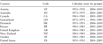
For our empirical analysis we use data compiled by Forey et al. (Reference Forey, Hamling, Hamling and Lee2011) in the International Smoking Statistics (ISS). The ISS data set consists of smoking prevalence data obtained from a large number of surveys. Rather than using data from an individual survey, we use prevalence data for standard age groups calculated by Forey et al. In the ISS there are three types of prevalence data: prevalence of smoking manufactured cigarettes, any cigarettes or any tobacco product. We consider here the prevalence of smoking any cigarettes, since many of the cohort studies consider cigarette smoking, but also since there are more data available for total cigarettes than for manufactured cigarettes. The standard age groups that are used are: 15–19, 20–24, … 80–84, 85+. In the ISS data calendar years are also in groups: 1951–55, …, 2006–2010. The available smoking prevalence data are summarised in table 1.

Table 1

Available prevalence data for smoking any cigarettes

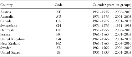
As we want to include as many data as possible in our empirical study, we do not exclude years for which smoking prevalence data are missing for a particular country. We therefore define for each calendar year t the set $$${\cal C}\left( {t} \right) $$$ of countries for which smoking prevalence data are available for this particular calendar year, for example, $$$ {\cal C}(1953)\, = \,\{ \:AT\:,\:DK\:,\:US\:\} $$$ . In the following we let $$$ {{s}_i}(t,x)\, \in \,[0,1] $$$ denote the smoking prevalence in country i, that is, the proportion of people aged x in year t in country i who smoke. The corresponding number of smokers is then approximately $$$ {{s}_i}(t,x){{E}_i}(t,x) $$$ . Note that $$$ {{s}_i}(t,x){{E}_i}(t,x) $$$ is actually an approximation for the smokers’ exposure-to-risk, that is the total number of person-years lived by smokers in the age interval [x, x + 1] during calendar year t.

The mortality data we use are the observed number of deaths D_i(t, x) and the exposure-to-risk E_i(t, x), which we obtained from the Human Mortality database, www.mortality.org. Unlike the ISS data, HMD data are available as “1 × 1-tables”, meaning that we have observations for each calendar year and each year of age.

Note that we do not observe death rates for smokers and non-smokers, separately. Observing these would simplify building a mortality model significantly. However, as far as we know, these data are not available in general. Also we do not observe cessation data, that is the proportion of non-smokers who used to smoke earlier in life.

Another issue with the available data is that smoking prevalence data are not available in a “1 × 1-table”. In general, prevalence data are only available for age groups as described earlier. To build a model based on annual observations we use linear interpolation to obtain annual prevalence data for each year of age, but it should be noted that this might not be the best way to deal with missing data. More sophisticated methods to estimate smoking prevalence in years with no observations are beyond the scope of this paper and are left for future research. For the linear interpolation applied here we assume that the observation for a particular age group in any five year period is the smoking prevalence for the middle age in this group in the middle year of that period. For example, we assume that the smoking prevalence in country i in the year 1973 for males aged 52, s_i (1973, 52), is given by the observed smoking prevalence for males aged 50 to 54 in the period 1971 to 1975. We then linearly interpolate across ages and calendar years to obtain a “1 × 1-table” containing smoking prevalence data for each calendar year and each age ranging from 17 (15–19 years old) to age 87 (aged 85+).

3 The Basic Model

To build a model for observed death rates, m_i(t, x), we start with the following obvious relationship for the number of deaths in country i

$${{D}_i}(t,x)\, = \,D_{i}^{N} (t,x)\, + \,D_{i}^{S} (t,x)$$

where $$$ D_{i}^{N} (t,x) $$$ and $$$ D_{i}^{S} (t,x) $$$ are the numbers of deaths among current non-smokers, and current smokers respectively, in country i aged x in year t. The total number of deaths is therefore the sum of the number of deaths among current smokers and the number of deaths among current non-smokers. We should mention here that D ^N and D ^S are not observed directly, as explained earlier. Also note that we do not distinguish between life-long non-smokers and former smokers. Both groups combined form the group of current non-smokers. We could divide the total population further taking into account other quantities, like number of cigarettes smoked per day, but with the limited data available, we choose to consider only current smokers and current non-smokers.

Using smoking prevalence data we can rewrite (1) as

$${ {{D}_i}(t,\:x)\, = \, & D_{i}^{N} (t,\:x)\, + \,D_{i}^{S} (t,\:x) \cr & = \,m_{i}^{N} (t,\:x)\,[1\:{\rm{ - }}\:{{s}_i}(t,\:x)]\,{{E}_i}(t,\:x)\, + \,m_{i}^{S} (t,\:x){{s}_i}(t,\:x){{E}_i}(t,\:x) \cr}$$

where s_i(t, x) denotes smoking prevalence, so that the number of smokers is s_i(t, x)E_i(t, x), and

$$m_{i}^{N} (t,x)\, = \,\frac{{D_{i}^{N} (t,x)}}{{[1\:{\rm{ - }}\:{{s}_i}(t,x)]{{E}_i}(t,x)}}$$

$$m_{i}^{S} (t,x)\, = \,\frac{{D_{i}^{S} (t,x)}}{{{{s}_i}(t,x){{E}_i}(t,x)}}$$

denote the death rates for non-smokers and smokers, respectively.

We then obtain for the death rates

$${{m}_i}(t,x)\, = \,\frac{{{{D}_i}(t,x)}}{{{{E}_i}(t,x)}}\, = \,m_{i}^{N} (t,x)\, + \,[m_{i}^{S} (t,x)\,\:{\rm{ - }}\,\:m_{i}^{N} (t,x)]{{s}_i}(t,x).$$

This equation does not form a model yet, and will still not allow us to estimate m ^N and m ^S. For that we will have to make some assumptions. The first assumption we make is

(A1) Non-smokers’ mortality in country i is the sum of general non-smokers’ mortality in all countries and a “country effect”

where the country effect is denoted by C_i(t, x) and refers to a country-specific quantity that affects non-smokers’ and smokers’ mortality in country i. This assumption implies that in the absence of smokers, the death rate in country i is given by $$$ {{m}_i}(t,x)\, = \,{{m}^N} (t,x)\, + \,{{C}_i}(t,x) $$$ . This is comparable to the model introduced by Li & Lee (Reference Li and Lee2005) although we are here looking at the death rates directly rather than log of death rates.

The second assumption we make deals with the effect of smoking:

(A2) Smoking has the same effect on mortality rates in all observed countries.

This assumption says that the excess mortality due to smoking is the same for every smoker in every country, although the actual death rates among smokers depend on the country effects, C_i(t, x), and also on general non-smokers’ mortality.

Combining assumpitons (A1) and (A2) we formulate the following model

$${{m}_i}(t,x)\, = \,{{m}^N} (t,x)\, + \,[{{m}^S} (t,x)\,{\rm{ - }}\,{{m}^N} (t,x)]{{s}_i}(t,x)\, + \,{{C}_i}(t,x)$$

where C_i(t, x) is the country specific effect, and $$$ [{{m}^S} (t,x)\,{\rm{ - }}\,{{m}^N} (t,x)] $$$ is the excess mortality caused by smoking. Note that in this model, m ^N and m ^S are not country specific. The model in (3) will serve as our basic model in the remainder of this paper.

We should mention here that the proposed model has a very simple structure, and that the effects of smoking on mortality and health are cumulative rather than immediate as our model might suggest. It is well known that smoking, and giving up smoking, do not cause an immediate change in survival probabilities of an individual. However, the model has been set up to allow us to estimate smokers’ and non-smokers’ death rates in multiple populations from the observations we have rather than describing the effects of smoking on the life expectancy of an individual life.

Our aim is now to estimate m ^N(t, x) and m ^S(t, x) in (3). As we wish to explain country-specific differences in mortality rates using smoking prevalence, we want to minimise the effect of other country-specific quantities, that is, we want to minimise the effect of C_i in (3). We will therefore choose estimates for m ^N and m ^S such that the following mean squared error

$$\:{\rm{MSE}}\:({{m}^S} (t,x),{{m}^N} (t,x))\, = \,\mathop{\sum}\limits_{i\, \in \,{\cal C}(t)} {{C}_i}{{(t,x)}^2} $$

is minimised for each year t and age x, where $$${\cal C}(t) $$$ denotes the set of countries for which prevalence data are available for calendar year t, compare section 2.1. Note that this is equivalent to treating C_i(t, x) as error terms in a linear regression model for each fixed age x and year t where the death rate m_i(t, x) is treated as a linear function of smoking prevalence s_i(t, x).

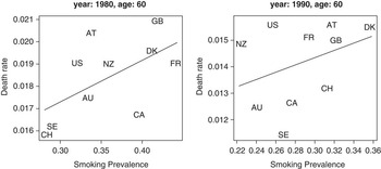
In figure 1 we show the data and the estimated linear regression function for years t = 1980 and t = 1990 for males aged 60. These plots are rather typical and plots for other years or ages exhibit the same problem, namely that the slope of the regression line is not significantly different from zero. However, although the slope is not particularly strong for most ages and years, it is positive for almost all ages and years.

Figure 1

The figure shows the observed (linearly interpolated) smoking prevalence (x-axis) and death rates (y-axis) in ten developed countries for males aged 60 in the calendar year 1980 (left plot) and 1990 (right plot), i.e. single age and single year. The straight line is the linear regression function estimated according to (3) and (4).

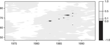
To investigate this relationship further we calculate the correlation between s_i(t, x) and m_i(t, x) for those years for which smoking data are available for all ten countries, that is, for 1973 to 1993, where we use the linear interpolated smoking prevalence data s_i(t, x) described earlier. Figure 2 shows the results as a contour plot of the correlation function

$$\gamma (t,x)\, = \,{\rm{Corr}}\:({{s}_i}(t,x),{{m}_i}(t,x))$$

where Corr denotes the empirical correlation function.

Figure 2

Contour plot of the correlation function $$$\gamma (t,x)$$$ . The small dark areas are period-age combinations for which a negative correlation between smoking prevalence and death rate have been observed.

We observe in figure 2 that there are only a small number of years in which negative correlations between smoking prevalence and death rates have been observed. This was for example the case in 1987 for males aged 73 with γ(1987, 73) = −0.132. However, the figure also indicates that for the vast majority of period-age combinations we find that $$$ \gamma (t,x) $$$ is positive. In fact, only about 1.3% of all correlations are negative (black area in figure 2), while about 39% of them are above 0.5 (white area in figure 2).

4 Further Modelling Assumptions

To develop a model for death rates as a function of time, age and smoking prevalence, we will now make further assumptions that link death rates observed over time and over ages to each other. Although, a large variety of assumptions is possible here, we will in the following consider only one particular assumption motivated by the empirical results found by Doll et al. (Reference Doll, Peto, Boreham and Sutherland2004):

(CSM) (Constant Smokers’ Mortality): There is no improvement in smokers’ mortality rates over time, that is $$$ {{m}^S} (t,x)\, = \,{{m}^S} (x) $$$ for all years t;

This is arguably a very strong assumption. However, taking into account that we are considering cohorts aged 50 to 87 in 1961 to 2005, that is, cohorts born between 1874 to 1955, we believe that this assumption might be justified by the results found by Doll et al. (Reference Doll, Peto, Boreham and Sutherland2004) for British Doctors born between 1900 and 1930. We should also mention that it is our aim for further research to consider alternative assumptions.

Under the (CSM) assumption our model becomes

$${{m}_i}(t,x)\, = \,{{m}^N} (t,x)\, + \,[{{m}^S} (x)\,\:{\rm{ - }}\,\:{{m}^N} (t,x)]{{s}_i}(t,x)\, + \,{{C}_i}(t,x).$$

We can now estimate m ^N(., x) and m ^S(x) for any fixed age x using Least-Squares Estimation where it is our aim to minimise the impact of country-specific effects. We now define the mean squared error as

$$\:{\rm{MSE}}\:({{m}^S}, {{m}^N} )\, = \,\mathop{\sum}\limits_t \mathop{\sum}\limits_{i\, \in \,{\cal C}(t)} {{({{C}_i}(t,x))}^2} $$

$$\; \; = \,\mathop{\sum}\limits_t \mathop{\sum}\limits_{i\, \in \,{\cal C}(t)} {{({{m}_i}(t,x)\,\:{\rm{ - }}\,\:{{m}^N} (t,x)\,\:{\rm{ - }}\,\:[{{m}^S} (x)\,\:{\rm{ - }}\,\:{{m}^N} (t,x)]{{s}_i}(t,x))}^2} $$

where it should be noted that $$$ {{m}^N} \, = \,({{m}^N} (1), \ldots, {{m}^N} (T)) $$$ . We now choose m ^S and m ^N such that MSE(m ^S, m ^N) is minimised. We should note here that the mean squared error as defined in (6) is not the mean of individual mean squared errors in single years, as this would require to divide each year-specific mean squared error by the number of countries considered in the particular year, which is not the same for all years. The MSE in (6) is the mean square error (up to a constant) for all years and countries. We have chosen this definition to avoid overweighting errors in years where data for only a few countries are available. Since the estimates for m ^S and m ^N obtained from minimising (6) are specific for a fixed age x we will suppress the depends on x in the following equations.

Differentiating MSE(m ^S, m ^N) in (7) with respect to m ^S and m ^N(t) for all years t shows that an explicit solution for a fixed age x is given by the solution of the following linear system of equations:

$${ 0\, & = \,\frac{\partial }{{\partial {{m}^S} }}\:{\rm{MSE}}\:({{m}^S}, {{m}^N} ) \cr & = \,2\mathop{\sum}\limits_t \mathop{\sum}\limits_{i\, \in \,{\cal C}(t)} \left( {{\rm{ - }}{{s}_i}(x)} \right)({{m}_i}(t)\,\:{\rm{ - }}\,\:{{m}^N} (t)\,\:{\rm{ - }}\,\:[{{m}^S} \,\:{\rm{ - }}\,\:{{m}^N} (t)]{{s}_i}(t)) \cr}$$

$$ { 0\, & = \,\frac{\partial }{{\partial {{m}^N} (t)}}\:MSE\:({{m}^S}, {{m}^N} ) \cr & = \,2\mathop{\sum}\limits_{i\, \in \,C(t)} ({{s}_i}(t)\,\:{\rm{ - }}\,\:1)({{m}_i}(t)\,\:{\rm{ - }}\,\:{{m}^N} (t)\,\:{\rm{ - }}\,\:[{{m}^S} \,\:{\rm{ - }}\,\:{{m}^N} (t)]{{s}_i}(t)) \cr} $$

or, equivalently,

$${{m}^S} \, = \,\frac{1}{{{{\Sigma }_t}{{\Sigma }_{i\, \in \,{\cal C}(t)}}s_{i}^{2} (t)}}\mathop{\sum}\limits_t \mathop{\sum}\limits_{i\, \in \,{\cal C}(t)} {{s}_i}(t)\left[ {{{m}_i}(t)\,\:{\rm{ - }}\,\:{{m}^N} (t)(1\,\:{\rm{ - }}\,\:{{s}_i}(t))} \right]$$

$${{m}^N} (t)\, = \,\frac{{{{\Sigma }_{i\, \in \,{\cal C}(t)}}(1\:\,{\rm{ - }}\,\:{{s}_i}(t)){{m}_i}(t)}}{{{{\Sigma }_{i\, \in \,{\cal C}(t)}}{{{(1\:\,{\rm{ - }}\,\:{{s}_i}(t))}}^2} }}\,\:{\rm{ - }}\,\:{{m}^S} \frac{{{{\Sigma }_{i\, \in \,{\cal C}(t)}}(1\,\:{\rm{ - }}\,\:{{s}_i}(t)){{s}_i}(t)}}{{{{\Sigma }_{i\, \in \,{\cal C}(t)}}{{{(1\,\:{\rm{ - }}\,\:{{s}_i}(t))}}^2} }}$$

Inserting (9) into (8) and solving the resulting equation for m ^S using the notation

$$\matrix{ {{A\, = \,\displaystyle\frac{{\rm{1}}}{{{{\Sigma }_t}{{\Sigma }_{i\, \in \,{\cal C}{\rm{(}}t{\rm{)}}}}\,s_{i}^{{\rm{2}}} {\rm{(}}t{\rm{)}}}}}} \bigg\{ \Sigma_t {{{\Sigma }_{i\, \in \,{\cal C}{\rm{(}}t{\rm{)}}}}S_i(t)m_i(t) } \qquad\qquad\qquad\qquad\qquad\qquad\qquad\qquad \cr \qquad\qquad\qquad\qquad{ {\rm{ - }}{{\Sigma }_t}\displaystyle\frac{{\left( {{{\Sigma }_{i\, \in \,{\cal C}{\rm{(}}t{\rm{)}}}}{\rm{(1}}\,\:{\rm{ - }}\,\:{{s}_i}{\rm{(}}t{\rm{))}}{{s}_i}{\rm{(}}t{\rm{)}}} \right) \left( {{{\Sigma }_{i\, \in \,{\cal C}{\rm{(}}t{\rm{)}}}}{\rm{(1}}\,\:{\rm{ - }}\,\:{{s}_i}{\rm{(}}t{\rm{))}}{{m}_i}{\rm{(}}t{\rm{)}}} \right)}}{{{{\Sigma }_{i\, \in \,{\cal C}{\rm{(}}t{\rm{)}}}}{{{{\rm{(1}}\:\,{\rm{ - }}\,\:{{s}_i}{\rm{(}}t{\rm{))}}}}^{\rm{2}}} }}} \right\bigg\} \qquad$$

and

$$ B\, = \,\frac{1}{{{{\Sigma }_t}{{\Sigma }_{i\, \in \,{\cal C}(t)}}s_{i}^{2} (t)}}\mathop{\sum}\limits_t {\frac{{{{{\left( {{{\Sigma }_{i\, \in \,{\cal C}(t)}}(1\:{\rm{ - }}\:{{s}_i}(t)){{s}_i}(t)} \right)}}^2} }}{{{{\Sigma }_{i\, \in \,{\cal C}(t)}}{{{(1\:{\rm{ - }}\:{{s}_i}(t))}}^2} }}} $$

we obtain the estimator $$$ {{\hat{m}}^S} $$$ for m ^S:

$${{m}^S} \, = \,A\, + \,{{m}^S} B\: \Rightarrow \:{{\hat{m}}^S} \, = \,\frac{A}{{1\:{\rm{ - }}\:B}}.$$

The estimator $$$ {{\hat{m}}^N} (t) $$$ for $$$ {{m}^N} (t) $$$ is then given by (9) where m ^S is replaced by $$$ A/(1{\rm{ - }}B) $$$ .

5 Empirical Results

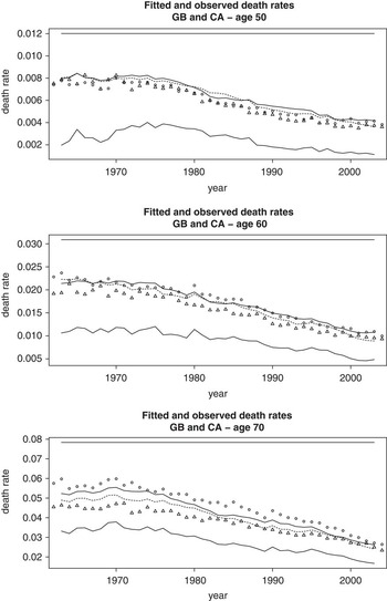
In the following we provide empirical estimates for m ^S and m ^N, and investigate the country effect. We start with investigating the fit of the model in (5) excluding the country effect. That is, we compare the observed death rates m_i(t, x) with $$$ {{\hat{m}}^N} (t,x)\, + \,[{{\hat{m}}^S} (x)\,{\rm{ - }}\,{{\hat{m}}^N} (t,x)]{{s}_i}(t,x) $$$ . As examples we show the rates for the United Kingdom (GB) and Canada (CA) for ages 50, 60 and 70 in figure 3. In these plots, the solid straight line at the top of each plot is the age specific smokers’ death rate, $$$ {{\hat{m}}^S} (x) $$$ , which does not change over time according to our assumption (CSM). The bottom solid line in each plot is the non-smokers’ death rates, $$$ {{\hat{m}}^N} (x,t) $$$ . Both of these rates are not country specific.

Figure 3

Observed and estimated death rates for the United Kingdom and Canada for different ages. The straight line at the top of each graph shows the estimated death rates for smokers, and the line at the bottom the rates for non-smokers. Circles and triangles correspond to the observed death rates for the UK and Canada, respectively. The solid and dashed line represent the fitted rates for the UK and Canada, respectively.

The circles and triangles represent the observed death rates m_i(t, x) for the United Kingdom and Canada, respectively, and the solid and dashed lines in the center of each plot are the fitted values $$$ {{\hat{m}}^N} (t,x)\, + \,[{{\hat{m}}^S} (x)\,{\rm{ - }}\,{{\hat{m}}^N} (t,x)]{{s}_i}(t,x) $$$ for the UK and Canada, respectively, where s_i(t, x) is the country-specific smoking prevalence.

We can see in these plots that the estimated death rates follow the actual death rates rather closely, but the observed death rates cannot be explained completely by smoking prevalence alone. The difference between the estimated and actual death rates is the country effect C_i(t, x) which we can now estimate by

$$ {{\hat{C}}_i}(t,x)\, = \,{{m}_i}(t,x)\,\:{\rm{ - }}\,\:({{\hat{m}}^N} (t,x)\: + \:[{{\hat{m}}^S} (x)\:\,{\rm{ - }}\,\:{{\hat{m}}^N} (t,x)]{{s}_i}(t,x)). $$

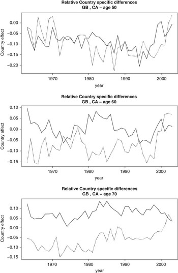
Rather than considering the country effect on its own, we are more interested in the relative country effect, that is, the ratio $$$ {{\hat{C}}_i}(t,x)/{{m}_i}(t,x) $$$ . We plot these ratios for ages 50, 60 and 70 in figure 4.

Figure 4

Relative country effects for the United Kingdom (solid line) and Canada (dashed line). The graphs show the estimated country effect relative to the observed death rates, that is, $$$ {{\hat{C}}_i}(t,x)/{{m}_i}(t,x) $$$ .

From these plots it is apparent that the country effect typically counts for about 5% to 20% of observed death rates in the UK and Canada. It is therefore a rather important factor. However, this also shows that the smokers’ and non-smokers’ death rates, which do not depend on the specific country, together with country-specific smoking prevalence data explain observed death rates to a large extent. We think these findings are rather surprising, taking into account the strong assumption we made about constant smokers’ mortality.

To use the proposed estimates to project death rates into the future would require to model the non-smokers’ death rate $$$ {{m}^N} (t,x) $$$ as well as the country effect. However, our empirical results indicate that the country effect could be modelled by a multi-dimensional stationary process, and that the non-stationary part, which is typically found in mortality models is here only present in the country-independent non-smokers’ death rate. Applying particular models to m ^N and C_i is not in the focus of this paper, and we therefore defer such an analysis to future research. To investigate the effect of smoking we will rather consider shocks to smoking prevalence observed in the past. This is done in the following section.

6 Scenarios and Annuity values

With the empirical estimates obtained in the last section we can now investigate the impact of smoking and country effects on survival rates and annuity values, starting with the impact of the country effect on the rate of survival. To this end we calculate the rate of survival to age x > 35 for the cohort aged 35 in 1961:

$$S(x,\,1961,\,35)\,\, = \prod\limits_{j\, = \,1}^{x{\rm{ - }}35} (1\,\:{\rm{ - }}\,\:{{m}_i}(1961\, + \,j,35\, + \,j))$$

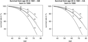
based on actually observed death rates m_i and compare it with the rate of survival based on estimated death rates, where we replace m_i(t, x) in (11) by $$$ {{\hat{m}}^N} (t,x)\, + \,[{{\hat{m}}^S} (x)\,{\rm{ - }}\,{{\hat{m}}^N} (t,x)]{{s}_i}(t,x) $$$ . These indexes are plotted for the UK and Canada in figure 5. In these plots the solid lines refer to the survival rates based on non-smokers’ (top line) and smokers’ (bottom line) death rates. The dashed line corresponds to the survival rates obtained from estimated death rates, and the circles are the survival rates based on actual death rates. The numbers are the survival rates at ages 50, 60 and 70 based on estimated death rates. We see in these plots that the country effect has only a small impact on the survival rates since the dashed line is very close to the circles, in particular, for Canada.

Figure 5

Survival rates from age 35 in 1961 for the UK and Canada. The topmost line represents the survival rate for non-smokers, and the bottom line the rates for smokers. The dashed line corresponds to the survival rates obtained from fitted death rates, and the circles are the survival rates for observed death rates. The numbers represent the values at age 50, 60 and 70. The middle numbers correspond to survival rates based on fitted death rates.

To investigate the impact of smoking we now consider a shock to smoking prevalence assuming that smoking prevalence from 1961 onwards was only 75% of its actual value, that is we consider an estimated death rate of

$$ {{\hat{m}}_i}(t,x)\, = \,{{\hat{m}}^N} (t,x)\, + \,{\bf {{0}}}{\bf {{.75}}}[{{\hat{m}}^S} (x)\:\,{\rm{ - }}\,\:{{\hat{m}}^N} (t,x)]{{s}_i}(t,x) $$

for the cohort aged 35 in 1961. Note that we ignore the country effect here completely.

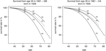
In figure 6 we plot the survivor rates for this scenario. It is apparent that survival rates to age 70 increased from 65 (GB) and 66 (CA) to 70. From these figures we can also see that survival rates would have increased to 79 for both countries if smoking prevalence had been 0. Comparing these differences to the differences caused by the country effect (see figure 5) shows the importance of smoking on survival rates.

Figure 6

Survival rates from age 35 in 1961 for the UK and Canada assuming a shock to smoking prevalence. The topmost line represents the survival rate for non-smokers, and the bottom line the rates for smokers. The dashed line corresponds to the survival rates obtained from fitted death rates assuming a reduced smoking prevalence (see section 6), and the circles are the survival rates for observed death rates. The numbers represent the values at age 50, 60 and 70. The middle numbers correspond to survival rates based on fitted death rates.

To investigate the impact on annuity values we again consider a shock to smoking prevalence by assuming that actual smoking prevalence is multiplied with a factor K, that is, we consider the following estimated death rates:

$${{\hat{m}}_i}(t,x)\, = \,{{\hat{m}}^N} (t,x)\, + \,{\bf {{K}}}[{{\hat{m}}^S} (x)\,{\rm{ - }}\,{{\hat{m}}^N} (t,x)]{{s}_i}(t,x).$$

Since we are interested in life annuities from retirement age, we consider these death rates for the cohort aged 65 in 1961.

We then calculate the rate of survival to age x > 65 for the cohort aged 65 in 1961:

$$ S(x,1961,65)\, = \,\prod\limits_{j\, = \,1}^{x{\rm{ - }}65} (1\,{\rm{ - }}\,{{m}_i}(1961\, + \,j,65\, + \,j)) $$

and based on these survival rates we find the values of life annuities in 1961 (max age = 110):

$$A(K,1961,x\, = \,65)\, = \,\mathop{\sum}\limits_{j\, = \,1}^{45} S(65\, + \,j,1961,65)\exp ({\rm{ - }}rj)$$

depending on the “smoking shock” K used for calculating the death rates $$$ {{\hat{m}}_i} $$$ .

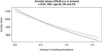
These annuity values are plotted in figure 7 as functions of K for the UK and Canada assuming an interest rate of 4% and a payment of £100.00 per annum in arrears.

Figure 7

Annuity values for a life annuity of £100.00 per annum paid in arrears for a male aged 65 in 1961 based on different scenarios for smoking prevalence. The interest rate is assumed to be 4%. The solid line represents annuity values for death rates in the United Kingdom, and the dashed line corresponds to Canada.

As expected any increase in smoking prevalence, results in a decreasing value of a life annuity since survival rates are lower. We also find that the values of life annuities would increase from around 900 to 1100 if smoking prevalence had been 0 since 1961.