1. Introduction
The marginal cost of using a trained large language model has fallen sharply since the release of ChatGPT in late 2022. At the same time, specialised AI hardware, especially GPUs and related infrastructure, appears to become economically obsolete much faster than conventional capital. This gives AI investment a distinctive economic character. Deploying AI requires large up-front expenditure, but once capacity is installed the marginal cost of many digital services is very low. Standard one-capital frameworks are not well suited to this combination. In particular, they have difficulty accounting for why spending booms in specialised hardware can unwind relatively quickly, and why a larger supply of low-cost digital services can materially affect consumption and welfare without necessarily changing aggregate factor shares very much.
The AI Index (2025) reports that the price of querying a model with GPT-3.5-level performance fell from around $20 to $0.07 per million tokens between November 2022 and October 2024.Footnote 1 At that lower price, a short text exchange costs only a fraction of a cent. These usage costs are now comparable in magnitude to the electricity needed for simple web-search (around 0.3 Wh), with recent measurement of median energy use for a Gemini text prompt at 0.24 Wh.Footnote 2 At the same time, API prices still differ widely across models and providers, and frontier multimodal systems remain much more expensive than low-cost tiers.Footnote 3 On the hardware side, investment in accelerators and data-centre infrastructure has shown pronounced boom-bust patterns, shaped in part by semiconductor cycles and repeated reassessments of useful economic life.
This paper studies those features in a neoclassical growth model with two reproducible assets, conventional capital and AI capacity. AI capacity is interpreted as the effective installed compute needed to deploy existing models, namely specialised hardware together with closely coupled software and infrastructure. The model weights themselves are non-rival, but installed capacity is rival and subject to congestion. Once in place, AI capacity generates a flow of digital services at low, though non-zero, marginal resource cost, and it also raises productivity in the tangible-goods sector. On the demand side, consumption is a CES aggregate of tangible goods and digital services. On the supply side, output is produced by a Cobb-Douglas technology in which AI capacity enters as an additional factor of production.
The allocation is characterised using a social planner problem with a capacity constraint and positive inference costs. In steady state, two user-cost conditions pin down the equilibrium. The first determines the user cost of conventional capital and implies a closed-form relationship between the steady-state stocks of conventional capital and AI capacity. The second determines the steady-state AI stock. Appendix A shows that, under mild assumptions, the relevant marginal-benefit map is strictly decreasing, which implies a unique interior solution.
To study adjustment dynamics, we log-linearise the Euler equations together with the accumulation equations around the steady state, while keeping investment endogenous in the resource constraint. This yields a reduced two-dimensional law of motion for the two capital stocks. For comparison, we also construct partial-equilibrium benchmarks in which investment is fixed at steady-state replacement levels, so that deviations decay mechanically at the underlying survival rates. Those benchmarks are useful because they isolate the role of durability. In the baseline calibration, passive decay alone implies a half-life of roughly seven quarters for AI capacity, compared with about eleven years for conventional capital. General-equilibrium dynamics differ because investment adjusts endogenously. For short-lived AI hardware, replacement flows are large relative to small stock deviations, so stock gaps can close much faster than passive depreciation alone would suggest. By contrast, when the economy begins with very little AI capacity, the optimal build-up is more gradual. Figures 1–3 compare these paths.
Two quantitative results are central. First, extending hardware life has a large effect on the steady-state AI stock and on the digital share of expenditure. In the baseline calibration, increasing the annual economic life of AI hardware from roughly three to four years raises the optimal AI stock by several tens of per cent and materially increases the share of digital services in consumption. Second, high depreciation creates a marked difference between passive and equilibrium adjustment. Because replacement flows are large, an excess stock of AI capacity can be worked off within a few quarters through relatively modest reductions in gross investment. The corresponding partial-equilibrium benchmark implies a much slower unwind. This helps account for the volatility often seen in hardware investment cycles.
The policy exercises use this mapping from hardware conditions into the model's primitives. A hardware tax or regulatory surcharge on compute can be represented as an increase in the effective depreciation rate of AI capacity, while longer service lives, repairability, or durability-enhancing measures work in the opposite direction. In the baseline calibration, a two-percentage-point increase in the quarterly economic depreciation rate reduces the optimal AI stock by around one-fifth. A symmetric improvement in hardware longevity raises lifetime welfare by around 0.36% in consumption-equivalent terms. Because AI hardware turns over quickly, the transition to the new steady state is also relatively fast.
The framework can also be extended in several directions without changing the basic two-asset structure. The paper briefly considers heterogeneous labour, nominal rigidities, and endogenous model size. These extensions are useful for distributional and monetary questions, but the main contribution of the paper is simpler. It is to show how rapid hardware obsolescence changes the macroeconomics of capital accumulation when AI capacity is treated as a distinct reproducible asset.
The remainder of the paper is organised as follows. Section 2 reviews the related literature. Section 3 sets out the environment and the planner's problem. Section 4 characterises the steady state and comparative statics. Section 5 discusses the calibration. Section 6 studies general-equilibrium adjustment and compares it with the partial-equilibrium benchmarks. Section 7 considers policy and measurement issues. Section 8 discusses extensions and robustness. Section 9 concludes.
2. Literature review
Macroeconomic analysis of artificial intelligence draws on three interconnected strands of research: (i) task-based automation and its labour-market consequences, (ii) the accumulation and measurement of intangible capital, and (iii) the empirical diffusion of robotics and foundation models. This section situates the present framework within those literatures and clarifies its distinctive contribution.
The potential for capital to substitute for labour in specific tasks, thereby influencing aggregate factor shares, has long been recognised. Zeira (Reference Zeira1998) showed how sequential task automation can compress the wage share unless the economy continually creates new labour-complementary activities. Building on that insight, Acemoglu and Restrepo (Reference Acemoglu and Restrepo2019) develop a tractable production function that combines displacement and reinstatement of labour, while subsequent studies explore the GE consequences of software-driven automation. Empirical work corroborates these mechanisms: exposure to industrial robots lowers employment and wages in US commuting zones (Acemoglu and Restrepo, Reference Acemoglu and Restrepo2020), with analogous displacement effects documented across European regions (Chiacchio et al. Reference Chiacchio, Petropoulos and Pichler2018). A common premise in much of this research, however, is that automated services are rivalrous, so their marginal production cost is comparable to the labour they replace. This paper instead models AI capacity as a high-depreciation capital asset: the underlying model weights are non-rival, but the installed hardware and associated infrastructure required to deploy them are rival and congestible, delivering very low marginal-cost services once in place.
That assumption links AI to the economic properties of intangible assets (software, designs, data) that can be replicated without diminishing their availability. Counting such spending as investment rather than intermediate expense substantially alters measurements of capital deepening and productivity growth (Corrado et al. Reference Corrado, Hulten and Sichel2009). Later work by Haskel and Westlake (Reference Haskel and Westlake2017) emphasises the scalability and non-rivalry of intangibles, helping to explain both the declining labour share (Karabarbounis and Neiman, Reference Karabarbounis and Neiman2014) and the rise of “superstar” firms. Yet while a subset of two-capital DSGE and growth models introduces separate tangible and intangible (or knowledge) stocks, they rarely admit analytically transparent dynamics and instead rely on balanced-growth characterisations or numerical solution methods (e.g. Romer, Reference Romer1990; Grossman and Helpman, Reference Grossman and Helpman1991; Aghion and Howitt, Reference Aghion and Howitt1992; McGrattan and Prescott, Reference McGrattan and Prescott2010). Furthermore, these models typically characterise “knowledge capital” as depreciating slowly, which contrasts sharply with the rapid obsolescence of AI hardware. By contrast, the present two-capital framework keeps the steady state analytically characterised even when the two-assets depreciate at very different rates: the user-cost conditions reduce the problem to a single monotone marginal-benefit map for AI capacity, and conventional capital is an explicit power function of the AI stock. Log-linearising the Euler equations and the accumulation rules around this steady state yields a two-dimensional system with interpretable eigenvalues, so that adjustment speeds and policy semi-elasticities can be expressed directly in terms of a small number of technology and preference parameters.
Global industrial-robot density more than doubled, from 69 to 151 robots per 10,000 manufacturing workers, between 2015 and 2022 (International Federation of Robotics, 2023). On the AI side, the Stanford Institute for Human-Centered Artificial Intelligence (2025) AI Index reports that the cost of querying a model delivering GPT-3.5-level performance fell from roughly $20 to $0.07 per million tokens within roughly two years (Nov 2022–Oct 2024). Capital outlays on specialised hardware such as GPUs follow similar boom-bust patterns tied to semiconductor fabrication cycles. The model’s short-run investment dynamics provide a theoretical counterpart to these rapid swings, linking their half-life to hardware obsolescence.
On the policy front, accelerated-depreciation allowances can tilt incentives toward automation (Acemoglu et al. Reference Acemoglu, Manera and Restrepo2020), and intangible booms may require counter-cyclical buffers to address financial-stability risks in AI hardware lending. Hence, bridging intangible capital with high depreciation is of direct policy relevance.
Relative to this literature, the paper combines AI's low marginal service cost and rapid hardware obsolescence in a tractable two-asset GE framework, and uses that framework to map technology primitives into macroeconomic and welfare outcomes.
3. The model
The economy lives in discrete time
 $t=0,1,2,\ldots$
and is populated by a representative household and perfectly competitive firms. It features two reproducible assets: conventional physical capital
 $K_t$
and a stock of AI capacity
 $M_t$
. The former depreciates slowly, the latter much faster. We interpret
 $M_t$
as effective installed AI capacity (specialised hardware and closely coupled infrastructure required to deploy existing models) whose economic depreciation is dominated by hardware obsolescence and intensive utilisation. Once installed, this capacity delivers digital services at low (but non-zero) marginal resource cost and, separately, raises the productivity of the tangible-goods sector.
Preferences and labour Household welfare is
 \begin{equation}\mathcal{U}_0=\sum _{t=0}^{\infty }\beta ^t \ln C_t, \qquad 0\lt \beta \lt 1,\end{equation}
where
 $C_t$
is a composite consumption index. To preserve the analytical focus on the capital block, we assume inelastic labour supply and normalise the endowment:
 \begin{equation*}L_t \equiv 1 \quad \text{for all } t.\end{equation*}
(Section 8 discusses an extension with endogenous labour.) Composite consumption aggregates tangible goods
 $C_t^{\textrm T}$
and digital services
 $D_t$
via
 \begin{equation}{C_t} = {\left[\theta {\mkern 1mu} {\left(C_t^{\textrm{T}}\right)^{{{\sigma - 1} \over \sigma }}} + (1 - \theta ){\mkern 1mu} D_t^{{{\sigma - 1} \over \sigma }}\right]^{{\sigma \over {\sigma - 1}}}},\qquad 0{\lt }\theta {{ \lt}}1,\;\sigma {{ \gt}}0,\end{equation}
with
 $\sigma$
the elasticity of substitution between tangible and digital streams.
Technology
Output of the tangible-goods sector is
 \begin{equation}Y_t=A\,K_t^{\alpha }\,M_t^{\zeta }\,L_t^{\,1-\alpha -\zeta }, \qquad 0\lt \alpha +\zeta \lt 1,\end{equation}
So the reproducible AI stock enters as a factor of production with elasticity
 $\zeta$
. Because the Cobb-Douglas exponents are primitive, the wage share equals
 $1-\alpha -\zeta$
and is invariant to movements in hardware costs or preferences.
AI capacity also enables a flow of digital services subject to capacity:
 \begin{equation}0\le D_t \le \psi \,M_t^{\phi },\qquad 0\lt \phi \le 1,\;\psi \gt 0,\end{equation}
while each unit of
 $D_t$
requires tangible resources (electricity, cooling, supervision) at marginal cost
 $\chi \gt 0$
.
Resource constraint and capital accumulation
Let
 $I^K_t$
and
 $X_t$
denote gross investment in
 $K_t$
and
 $M_t$
, respectively. Goods feasibility is
 \begin{equation}C_t^{\textrm T}+I^K_t+X_t+\chi \,D_t=Y_t,\end{equation}
and the two-assets evolve according to
 \begin{align} K_{t+1} &=(1-\delta )\,K_t+I^K_t, 0\lt \delta \lt 1, \end{align}
 \begin{align} M_{t+1} &=(1-\delta _M)\,M_t+X_t, 0\lt \delta _M\lt 1. \end{align}
Planner’s problem, multipliers and optimality conditions
Because markets are competitive and there are no externalities, the decentralised allocation coincides with the solution to a social planner who chooses
 $\{C_t^{\textrm T},D_t,I^K_t,X_t\}_{t\ge 0}$
to maximise (1) subject to (2)–(7) and given
 $(K_0,M_0)$
. Let
 $\lambda _t$
be the current-value multiplier on (5) (goods units) and
 $\mu _t\ge 0$
the multiplier on the capacity constraint in (4). The FOC with respect to tangible consumption implies
 \begin{equation*}{\lambda _t}={{\partial {{\mathcal U}_t}} \over {\partial {C_t}}}{\mkern 1mu} {{\partial {C_t}} \over {\partial C_t^{\textrm{T}}}}={1 \over {{C_t}}}{\mkern 1mu} {{\partial {C_t}} \over {\partial C_t^{\textrm{T}}}}.\end{equation*}
Define the intratemporal marginal rate of substitution
 \begin{equation*}{\textrm{MR}}{{\textrm{S}}_t} \equiv {{\partial {C_t}/\partial {D_t}} \over {\partial {C_t}/\partial C_t^{\textrm{T}}}} = {{1 - \theta } \over \theta }{\left( {{{C_t^{\textrm{T}}} \over {{D_t}}}} \right)^{1/\sigma }}.\end{equation*}
The Kuhn-Tucker conditions yield:
(i) Consumption-services mix with capacity
 \begin{equation}\textrm{MRS}_t\begin{cases} =\;\chi , & \text{if capacity is slack}\;\;\big(D_t\lt \psi M_t^{\phi },\;\mu _t=0\big),\\[4pt] \ge \;\chi , & \text{if capacity binds}\;\;\big(D_t=\psi M_t^{\phi },\;\mu _t\ge 0\big). \end{cases}\end{equation}
(ii) Euler equation for tangible capital
 \begin{equation}{\lambda _t} = \beta {\mkern 1mu} {\lambda _{t + 1}}\left[(1 - \delta ) + \alpha {\mkern 1mu} {{{Y_{t + 1}}} \over {{K_{t + 1}}}}\right]\!.\end{equation}
(iii) Euler equation for AI capacity
A unit of
 $M_{t+1}$
survives with probability
 $(1-\delta _M)$
and yields two dividends at
 $t+1$
: a production dividend inside (3) and a services dividend equal to the net value of the induced extra flow of
 $D_{t+1}$
beyond its resource cost
 $\chi$
. The envelope condition is
 \begin{equation}{\lambda _t} = \beta {\mkern 1mu} {\lambda _{t + 1}}\left[(1 - {\delta _M}) + \zeta {\mkern 1mu} {{{Y_{t + 1}}} \over {{M_{t + 1}}}} + \max \left\{ {0,{\textrm{MR}}{{\textrm{S}}_{t + 1}} - \chi } \right\}{\mkern 1mu} \phi {\mkern 1mu} \psi {\mkern 1mu} M_{t + 1}^{\phi - 1}\right]\!.\end{equation}
The services term vanishes under slack capacity (
 $\textrm{MRS}_t=\chi$
) and is positive when capacity binds (
 $\textrm{MRS}_t\gt \chi$
).
Focus of the analysis (regime).
Given the high productivity of AI services and the specialised hardware required, we focus on the empirically relevant binding-capacity regime:
 \begin{equation*}D_t=\psi M_t^{\phi }\quad \text{and}\quad \textrm{MRS}_t\gt \chi \end{equation*}
for the baseline results. Slack-capacity formulas are collected in the appendix, and the two regimes yield piecewise-defined local dynamics when the Euler system is linearised.
Steady state
Let
 $K_{t+1}=K_t\equiv K^*$
,
 $M_{t+1}=M_t\equiv M^*$
and
 $D^*=\psi (M^*)^{\phi }$
(binding). The Euler conditions become
 \begin{align} 1 &= \beta \left[(1 - \delta ) + \alpha {\mkern 1mu} {{{Y^*}} \over {{K^*}}}\right]\!, \end{align}
 \begin{align} 1 &= \beta \left[(1 - {\delta _M}) + \zeta {\mkern 1mu} {{{Y^*}} \over {{M^*}}} + ({\textrm{MR}}{{\textrm{S}}^*} - \chi ){\mkern 1mu} \phi {\mkern 1mu} \psi {\mkern 1mu} {({M^*})^{\phi - 1}}\right]\!, \end{align}
with
 $Y^*=A\,(K^*)^{\alpha }\,(M^*)^{\zeta }$
(using
 $L_t=1$
) and
 \begin{equation*}{\textrm{MR}}{{\textrm{S}}^*} = {{1 - \theta } \over \theta }{\left( {{{{C^{{\textrm{T}}*}}} \over {{D^*}}}} \right)^{1/\sigma }},\qquad {C^{{\textrm{T}}*}} = {Y^*} - \delta {K^*} - {\delta _M}{M^*} - \chi {D^*}.\end{equation*}
In the binding-capacity regime, the steady state is the solution to the simultaneous system composed of (11)–(12), the feasibility condition above, the production function (3), and the definition of
 $\textrm{MRS}^*$
. The first equality pins down the user cost of tangible capital; the second equates the price of one unit of AI capacity to the present value of its resale plus dividends. The key property for uniqueness is that the right-hand side of (12), the discounted marginal benefit of capacity, is strictly decreasing in
 $M^*$
. As shown formally in Appendix A, this monotonicity is preserved once the general-equilibrium adjustment of
 $\textrm{MRS}^*$
is accounted for, guaranteeing a unique interior solution.Footnote
4
Lower
 $\chi$
weakly increases the likelihood that capacity binds and raises the services dividend in (12); a lower
 $\delta _M$
or higher
 $\zeta$
increases the production dividend. In all three cases, the optimal
 $M^*$
rises. (Closed-form elasticities reported later are computed under binding capacity and rely on the appendix monotonicity result.)
Local dynamics
Let
 $k_t\equiv \ln K_t-\ln K^*$
and
 $m_t\equiv \ln M_t-\ln M^*$
. Log-linearising the Euler block together with (6)–(7) around the steady state yields a two-dimensional linear system
 \begin{equation}\begin{bmatrix}k_{t+1}\\ m_{t+1}\end{bmatrix} =J\,\begin{bmatrix}k_t\\ m_t\end{bmatrix},\end{equation}
where
 $J$
is the Jacobian of the law of motion for
 $(K_t,M_t)$
evaluated at
 $(K^*,M^*)$
. Because the marginal-utility co-state depends on investment through feasibility, the log-linearised Euler block is second order in
 $(k_t,m_t)$
, and the two-dimensional law of motion
 $x_{t+1}=Jx_t$
is obtained by forming the companion system and selecting the stable manifold (Appendix B). Each entry of
 $J$
is a unit-free elasticity built from
 $(\alpha ,\zeta ,\sigma ,\theta ,\delta ,\delta _M,\phi ,\psi ,\chi )$
and steady-state ratios. The coefficients are regime-dependent: (i) if capacity is slack (
 $\textrm{MRS}_t=\chi$
), the services term envelopes out and the off-diagonal elements reflect only the production channel (proportional to
 $\alpha \zeta$
); the system becomes block-diagonal only when, in addition,
 $\zeta =0$
. (ii) Under binding capacity (
 $\textrm{MRS}_t\gt \chi$
), an extra term proportional to
 $(\textrm{MRS}^*-\chi )\,\phi$
enters the
 $M$
equation. Appendix B describes the construction and sign structure of
 $J$
in more detail. Section 6 uses the eigenvalues of
 $J$
to characterise general-equilibrium adjustment speeds and to compare them with the simpler partial-equilibrium geometric benchmarks driven directly by the depreciation rates
 $(\delta ,\delta _M)$
.
AI capacity
 $M_t$
represents specialised hardware and associated infrastructure, which are rival inputs. The model abstracts from the micro-allocation of that compute between two uses, raising productivity in tangible production (Eq. [3]) and serving digital demand (Eq. [4]), by allowing the same stock to play both roles at the macro level. This abstraction preserves the tractability of the two-asset core while capturing the dual economic role of AI capital. A variant that explicitly allocates hardware across uses,
 $M_t=M_t^{Y}+M_t^{D}$
with
 $D_t\le \psi (M_t^{D})^{\phi }$
, equalises marginal values across uses within the period and leaves the state dimension unchanged; its algebraic details are available on request.
4. Steady-state allocation and comparative statics
In the binding-capacity regime (
 $D_t=\psi M_t^{\phi }$
), the steady state is characterised by the two user-cost equalities
 \begin{align} 1 &= \beta \left[(1 - \delta ) + \alpha {\mkern 1mu} {{{Y^*}} \over {{K^*}}}\right]\!, \end{align}
 \begin{align} 1 &= \beta \left[(1 - {\delta _M}) + \zeta {\mkern 1mu} {{{Y^*}} \over {{M^*}}} + ({\textrm{MR}}{{\textrm{S}}^*} - \chi ){\mkern 1mu} \phi \psi {\mkern 1mu} {({M^*})^{\phi - 1}}\right]\!, \end{align}
where
 $D^{*}=\psi \,(M^{*})^{\phi }$
and
 \begin{equation*}{\textrm{MR}}{{\textrm{S}}^*} = {{1 - \theta } \over \theta }{\left( {{{{C^{{\textrm{T}}*}}} \over {{D^*}}}} \right)^{1/\sigma }},\qquad {C^{{\textrm{T}}*}} = {Y^*} - \delta {K^*} - {\delta _M}{M^*} - \chi {D^*}.\end{equation*}
Output is
 $Y^{*}=A\,(K^{*})^{\alpha }\,(M^{*})^{\zeta }$
(using
 $L=1$
).
Analytical mapping for
 $\boldsymbol{K}^{\boldsymbol{*}}$
Equation (14) pins down the user cost of tangible capital and implies a simple power-law relationship between
 $K^{*}$
and
 $M^{*}$
:
 \begin{equation}{K^*} = {[\Xi {\mkern 1mu} {({M^*})^\zeta }]^{1/(1 - \alpha )}},\qquad \Xi = {{\alpha {\mkern 1mu} A} \over {{\beta ^{ - 1}} - (1 - \delta )}}.\end{equation}
Hence, conventional capital is an explicit function of the AI stock: once
 $M^{*}$
is known, both
 $K^{*}$
and
 $Y^{*}$
follow immediately from (16) and the production function. Substituting (16) into (15) collapses the steady-state problem to a single scalar equation in
 $M^{*}$
, where the right-hand side (the discounted marginal benefit of capacity, comprising resale, production, and net services) is strictly decreasing in
 $M^{*}$
. As shown in Appendix A, this monotonicity is preserved even when the endogenous term
 $\textrm{MRS}^{*}$
adjusts with
 $M^{*}$
, guaranteeing a unique interior solution for AI capacity. In this sense, the steady state is analytically characterised: one user-cost condition delivers the explicit mapping
 $K^{*}(M^{*})$
, and the other determines
 $M^{*}$
as the unique root of a monotone marginal-benefit map.
Factor-income shares
Under perfect competition the real wage equals the marginal product of labour,
 $w^{*}=(1-\alpha -\zeta )\,Y^{*}$
. Measured against value added
 $Y^{*}$
the labour share is therefore
 \begin{equation}s^{*}_{L}=1-\alpha -\zeta .\end{equation}
Because the Cobb-Douglas exponents
 $(\alpha ,\zeta )$
are treated as primitive technology parameters,
 $s^{*}_{L}$
is invariant to movements in
 $\delta _M$
,
 $\chi$
or
 $\sigma$
in the baseline model. Put differently, the constancy of the aggregate labour share is an assumption built into the production structure: shifts in hardware longevity, inference costs, or substitution elasticities affect the scale of AI capital and the composition of expenditure, but do not alter the wage share unless
 $\zeta$
itself is allowed to vary. Extensions in which the effective output elasticity of AI capacity evolves with
 $M^{*}$
(for example, via organisational capital or learning-by-doing) would naturally generate time-varying labour shares, but those mechanisms are kept outside the baseline for tractability.
Comparative statics (signs)
Let
 $\mathcal{S}\equiv \{K^{*},M^{*},Y^{*},D^{*}\}$
. Differentiating the steady-state system implicitly and using the monotonicity result in Appendix A yields unambiguous signs for the key technology primitives:
 \begin{equation*}{{\partial {M^*}} \over {\partial {\delta _M}}}\lt 0,\qquad {{\partial {M^*}} \over {\partial \chi }}\lt 0,\qquad {{\partial {M^*}} \over {\partial \zeta }}{\gt}0.\end{equation*}
A lower economic depreciation rate for AI hardware (
 $\delta _M$
) or a higher output elasticity of AI capacity (
 $\zeta$
) both increase the marginal benefit of holding
 $M$
, raising the steady-state AI stock. A higher marginal resource cost of digital services (
 $\chi$
) reduces the net services dividend in (15) and therefore lowers
 $M^{*}$
.
Changes in the elasticity of substitution
 $\sigma$
operate only through
 $\textrm{MRS}^{*}$
and thus have an a priori ambiguous effect on
 $M^{*}$
; the sign depends on the steady-state ratio
 $C^{\textrm T*}/D^{*}$
and the calibration of
 $(\theta ,\sigma )$
. Once
 $M^{*}$
is determined,
 $K^{*}$
follows from (16) and
 $Y^{*}$
from the production function, while
 $D^{*}$
is pinned down by capacity,
 $D^{*}=\psi (M^{*})^{\phi }$
.
Interpretation
Hardware longevity (
 $\delta _M$
) and the marginal resource cost of inference (
 $\chi$
) are technological primitives; together with the production elasticity
 $\zeta$
they scale the optimal stock of AI capacity and, via the CES aggregator, the steady-state share of digital services in expenditure. Increases in longevity or productivity push up
 $M^{*}$
,
 $K^{*}$
and
 $Y^{*}$
, and raise the digital share, whereas higher marginal resource costs pull in the opposite direction. None of these movements, however, affects the labour share
 $1-\alpha -\zeta$
in (17) as long as the Cobb-Douglas exponents are fixed. The next section calibrates the parameters to recent evidence and reports the implied steady-state levels, digital expenditure shares, and the ratios that enter the dynamics and policy analysis.
5. Calibration
We calibrate the model to advanced economies circa mid-2025, with particular attention to the AI-capacity block. The model is solved at a quarterly frequency, with period parameters obtained from annual targets.Footnote
5
Throughout, we adopt the empirically relevant binding-capacity regime (
 $D_t=\psi M_t^{\phi }$
with
 $\textrm{MRS}_t\gt \chi$
), so the shadow price of digital services
 $p_D\equiv \textrm{MRS}_t$
enters the Euler condition for
 $M_t$
and the steady state. As in Section 3, the labour endowment and technology level are normalised to
 $L_t=1$
and
 $A=1$
. For the baseline parameter vector, we verify ex post that the steady state indeed lies in the binding regime (Appendix A).
5.1 Foundational macro parameters
The annual discount factor
 $\beta _a$
targets a long-run real interest rate of 1% per year,
 $\beta _a=1/1.01\approx 0.99$
, consistent with official US long-run assessments in the low single digits.Footnote
6
This implies a quarterly discount factor
 \begin{equation*}\beta = \beta _a^{1/4} \approx 0.9975. \end{equation*}
The tangible capital share is fixed at
 $\alpha =0.30$
, a conventional value in growth/RBC calibrations and consistent with PWT-based labour-share evidence for advanced economies.Footnote
7
For the depreciation rate of tangible capital we set
 $\delta _a=0.06$
annually, in line with implied geometric rates across private fixed assets using BEA fixed-asset accounts and related methodology notes.Footnote
8
This implies a quarterly rate
 \begin{equation*}\delta = 1 - (1-\delta _a)^{1/4} \approx 0.0154. \end{equation*}
5.2 AI-capacity block
Economic depreciation of AI capacity
We choose an annual rate
 $\delta _{M,a}=0.33$
(an economic service life of roughly three years) to capture the rapid obsolescence and heavy utilisation of specialised accelerators. This is an economic rate, distinct from accounting lives, which the major hyperscalers have extended to six years for servers (and networking) in 2023–2024.Footnote
9
Market data strongly supports this rapid decay. Historical resale pricing for the Nvidia V100 (2017–2020 cycle) indicates a value loss of approximately 45% within two years of release. More recently, spot market rental rates for H100 GPUs, a direct proxy for the asset’s economic yield, declined by roughly 50% in the first eight months of 2024 alone (GPUutils, 2024). This rapid depreciation reflects continuing improvements in GPU price-performance and the resulting obsolescence of older vintages (Hobbhahn and Besiroglu, Reference Hobbhahn and Besiroglu2022).
The quarterly depreciation rate used in the model is
 \begin{equation*}\delta _M = 1-(1-\delta _{M,a})^{1/4} \approx 0.0953, \end{equation*}
So the quarterly survival rate of installed AI capacity is about
 $1-\delta _M\approx 0.905$
. This survival rate defines the PE passive-decay benchmark against which the GE dynamics are compared in Section 6. It also governs the steady-state replacement flow
 $\delta _M M^{*}$
, which is large enough that the planner can close small stock gaps much faster than passive decay alone, as the impulse responses in Figures 1, 2, and 3 illustrate.
AI in production
The elasticity of AI capacity in the goods technology is set to
 $\zeta =0.06$
as a transparent scenario capturing a modest but non-trivial contribution of
 $M_t$
to value added. Because macro evidence is nascent, we treat
 $\zeta$
as a disciplined scenario parameter rather than a tight estimate and report sensitivity in robustness checks.
Digital services technology
We set
 $\phi =0.7$
to capture aggregate congestion and bottlenecks (energy, cooling, bandwidth, engineering) that temper the micro-level scalability of inference. This curvature helps ensure a well-defined steady state under binding capacity and matters for the strength of the services dividend in the AI Euler equation, but does not affect the qualitative conclusions about relative adjustment speeds.
Marginal resource cost of services
We calibrate a small positive
 $\chi$
consistent with recent evidence that the resource cost of LLM inference is extremely low. The AI Index (2025) documents a drop in GPT-3.5-level inference prices from about $20 to $0.07 per million tokens during Nov 2022–Oct 2024, and Google reports a median inference energy of roughly
 $0.24$
Wh for a text prompt.Footnote
10
At retail electricity prices around $0.10–0.15 per kWh, this corresponds to energy costs of the order of
 $10^{-5}$
dollars per prompt, highlighting just how small the physical resource cost is.
Because output in the model is measured in abstract goods units, there is no unique mapping from these dollar figures to
 $\chi$
. We therefore set
 $\chi =0.006$
as a conservative scenario value: this places the marginal resource cost of digital services well below unity in goods units, ensures that the steady state lies in the binding-capacity regime (
 $p_D^*\gt \chi$
), and implies resource use for digital services that is easily reconciled with the inference-cost numbers above under any plausible normalisation of
 $Y^*$
. The main results are robust to small perturbations around this value.
5.3 Consumption aggregator and digital-share target
We set the elasticity of substitution between tangible goods and digital services to
 $\sigma =1.5$
. This implies that the two streams are gross substitutes (
 $\sigma \gt 1$
), consistent with estimates for related categories such as home-production substitution (often cited around 1.5–1.8).
We target a baseline digital expenditure share of
 $s_D=0.10$
. The BEA Digital Economy Satellite Account estimates that the digital economy accounted for about 10% of US GDP in 2022 (the latest benchmark year). In the model,
 $s_D$
is the expenditure share of digital services in the composite consumption aggregator rather than the value-added share of a “digital sector”. We use the BEA figure as an order-of-magnitude target for this consumption share, recognising that the two concepts are not identical.
Given the exogenous parameters (including
 $\chi$
), we jointly calibrate the CES weight
 $\theta$
and the service-efficiency parameter
 $\psi$
to match the target
 $s_D$
in the steady state. Because capacity binds, the shadow price
 $p_D^*=\textrm{MRS}^*$
is endogenous. For given
 $(\theta ,\psi )$
we solve for the steady state, obtain
 $p_D^*$
, and then update
 $\theta$
so that the implied expenditure share satisfies
 \begin{equation*}{{{s_D}} \over {1 - {s_D}}} = {\left( {{{1 - \theta } \over \theta }} \right)^\sigma }{\left( {p_D^*} \right)^{1 - \sigma }} \Rightarrow \theta = {1 \over {1 + {{\left[ {\left( {{s_D}/\left( {1 - {s_D}} \right)} \right){{\left( {p_D^*} \right)}^{\sigma - 1}}} \right]}^{1/\sigma }}}}.\end{equation*}
Simultaneously, we adjust
 $\psi$
so that
 $D^*=\psi \,(M^*)^{\phi }$
matches the level of digital expenditure consistent with
 $s_D$
and the resource constraint. In practice, this two-dimensional fixed-point problem converges quickly: starting from a reasonable guess for
 $(\theta ,\psi )$
, a few iterations are enough to hit the expenditure-share target to numerical tolerance. This procedure ensures that the calibration is fully consistent with the binding-capacity Euler condition and with the targeted digital share.
External price checks
Published API prices vary by model and date: low-cost tiers such as Gemini Flash are now only a small multiple of benchmark resource costs, while frontier multimodal models remain substantially more expensive per token. We do not attempt to match any specific price series; instead, we use these figures as external reasonableness checks that the chosen combination of
 $\chi$
,
 $p_D^*$
, and the digital share
 $s_D$
lies in a plausible range given observed API pricing and energy-use statistics.
6. Adjustment dynamics
This section characterises the transition dynamics of the two-asset economy. The distinct depreciation rates of conventional capital and AI capacity imply widely separated adjustment speeds. We start from the linearised GE system derived in Section 3 and Appendix B, show how its eigenvalues relate to the underlying depreciation rates, and then compare the resulting impulse responses with simple PE (PE) geometric benchmarks. Throughout, time is measured in quarters and all parameters are the quarterly values implied by the calibration in Section 5.
6.1 Linear general equilibrium dynamics
Let
 $k_t \equiv \ln K_t - \ln K^{*}$
and
 $m_t \equiv \ln M_t - \ln M^{*}$
denote log deviations of the two capital stocks around the steady state
 $(K^{*},M^{*})$
described in Section 4. Log-linearising the tangible-capital Euler equation (9), the AI-capacity Euler equation (10) and the accumulation equations (6) and (7) around
 $(K^{*},M^{*})$
yields the two-dimensional linear system
 \begin{equation}\begin{bmatrix} k_{t+1} \\ m_{t+1} \end{bmatrix} = J \begin{bmatrix} k_t \\ m_t \end{bmatrix}, \qquad J \equiv \begin{bmatrix} J_{KK} & J_{KM} \\ J_{MK} & J_{MM} \end{bmatrix},\end{equation}
where
 $J$
is the Jacobian of the law of motion for
 $(K_t,M_t)$
evaluated at the steady state. Each entry of
 $J$
is a unit-free elasticity built from the primitive parameters
 $(\alpha ,\zeta ,\sigma ,\theta ,\delta ,\delta _M,\phi ,\psi ,\chi )$
and steady-state ratios such as
 $Y^{*}/K^{*}$
and
 $Y^{*}/M^{*}$
. Because investment is endogenous in the feasibility constraint, the Euler block is second order in
 $(K_t,M_t)$
; the reduced two-state law of motion
 $x_{t+1}=Jx_t$
is obtained by forming a companion system and selecting the stable eigenspace (Appendix B). Here, we focus on the economic content of the resulting GE dynamics and compare them with PE benchmarks that hold investment at replacement levels.
Intuitively, a positive deviation in
 $K_t$
lowers the marginal product of capital and hence the gross return (user cost) on tangible capital, which reduces the incentive to invest and induces a gradual return of
 $K_{t+1}$
towards
 $K^{*}$
; this effect, together with depreciation, determines
 $J_{KK}$
. The term
 $J_{MM}$
is governed by the high depreciation rate of AI capacity, the diminishing marginal product of
 $M$
, and the curvature of the congestion term in the services dividend. The off-diagonal terms reflect GE linkages. Through the Cobb-Douglas technology, higher AI capacity raises the marginal product of tangible capital and vice versa, generating terms proportional to
 $\alpha \zeta$
. When capacity binds, the services dividend contributes an additional cross-effect proportional to
 $(\text{MRS}^{*}-\chi )\phi$
; when capacity is slack that component is absent.
Let
 $\lambda _1$
and
 $\lambda _2$
denote the eigenvalues of
 $J$
, ordered so that
 $0 \lt \lambda _1 \leq \lambda _2 \lt 1$
. Because the model is saddle-path stable (Appendix B), both eigenvalues lie strictly inside the unit circle. The associated half-lives are
 \begin{equation*}{t_{1/2}}({\lambda _i}) = {{\ln 0.5} \over {\ln {\lambda _i}}},\qquad i = 1,2.\end{equation*}
In the baseline calibration of Section 5, the fast eigenvalue
 $\lambda _1$
is near zero (
 $\approx 7.4\times 10^{-6}$
), implying an extremely rapid adjustment mode through which the planner eliminates most stock deviations within one or two quarters by re-optimising gross investment. The slow eigenvalue
 $\lambda _2\approx 0.980$
governs the gradual convergence of tangible capital. Appendix B reports the full numerical Jacobian. For comparison, the PE survival rates are
 $1-\delta _M\approx 0.905$
and
 $1-\delta \approx 0.985$
; the GE eigenvalues diverge from these benchmarks because the linearisation keeps investment endogenous in the feasibility constraint. Economically, the system decomposes into a fast mode through which the planner exploits the large replacement flows of short-lived AI hardware to close stock gaps quickly, and a slow mode associated with the sluggish adjustment of tangible capital.
Given an initial deviation
 $x_0 \equiv (k_0,m_0)^{\prime }$
, the GE solution is
 \begin{equation}x_t = J^t x_0 = \omega _1 \lambda _1^t v_1 + \omega _2 \lambda _2^t v_2,\end{equation}
where
 $v_i$
is the eigenvector associated with
 $\lambda _i$
and the weights
 $\omega _i$
are determined by the initial condition. The fast mode dominates the short-run response of AI capacity and the digital block; the slow mode governs the protracted adjustment of tangible capital and output.
6.2 Partial equilibrium geometric benchmarks
While (18) describes the exact linearised GE dynamics, it is useful to have a simpler benchmark that makes the role of depreciation rates completely transparent. Following the heuristic in the original version of the paper, consider a PE experiment in which investment in each asset is fixed at its steady-state replacement level. The capital-stock equations then become
 \begin{align*}K_{t+1} &= (1-\delta )\,K_t + \delta K^{*}, \notag\\ M_{t+1} &= (1-\delta _M)\,M_t + \delta _M M^{*}.\end{align*}
Expressed in log deviations, a first-order approximation delivers
 \begin{equation}k_{t+1} \approx (1-\delta )\,k_t, \qquad m_{t+1} \approx (1-\delta _M)\,m_t.\end{equation}
The PE dynamics thus consist of two independent geometric decay processes, with roots equal to the survival rates of the respective capital stocks.
Under the baseline quarterly calibration
 $(\delta ,\delta _M) = (0.0154,0.0953)$
, these roots are
 \begin{equation*}\text{Fast root (AI capacity)}:\quad 1-\delta _M \approx 0.905, \qquad \text{Slow root (tangible capital)}:\quad 1-\delta \approx 0.985. \end{equation*}
The implied half-lives are
 \begin{equation}t_{1/2}^M = {{\ln 0.5} \over {\ln (1 - {\delta _M})}} \approx 6.9\;{\textrm{quarters}}\;( \approx 1.7{\textrm{ years}}),\quad t_{1/2}^K = {{\ln 0.5} \over {\ln (1 - \delta )}} \approx 44.8\;{\textrm{quarters}}\;( \approx 11{\textrm{ years}})\end{equation}
These PE half-lives provide a transparent yardstick for passive depreciation-driven decay when investment is held at its steady-state replacement level. In the GE linearisation, investment re-optimisation introduces a much faster adjustment mode for AI capacity, so equilibrium convergence can be substantially quicker than passive decay, especially for high-depreciation hardware. Appendix B reports the Jacobian and eigenvalues.
6.3 Impulse responses: GE versus PE
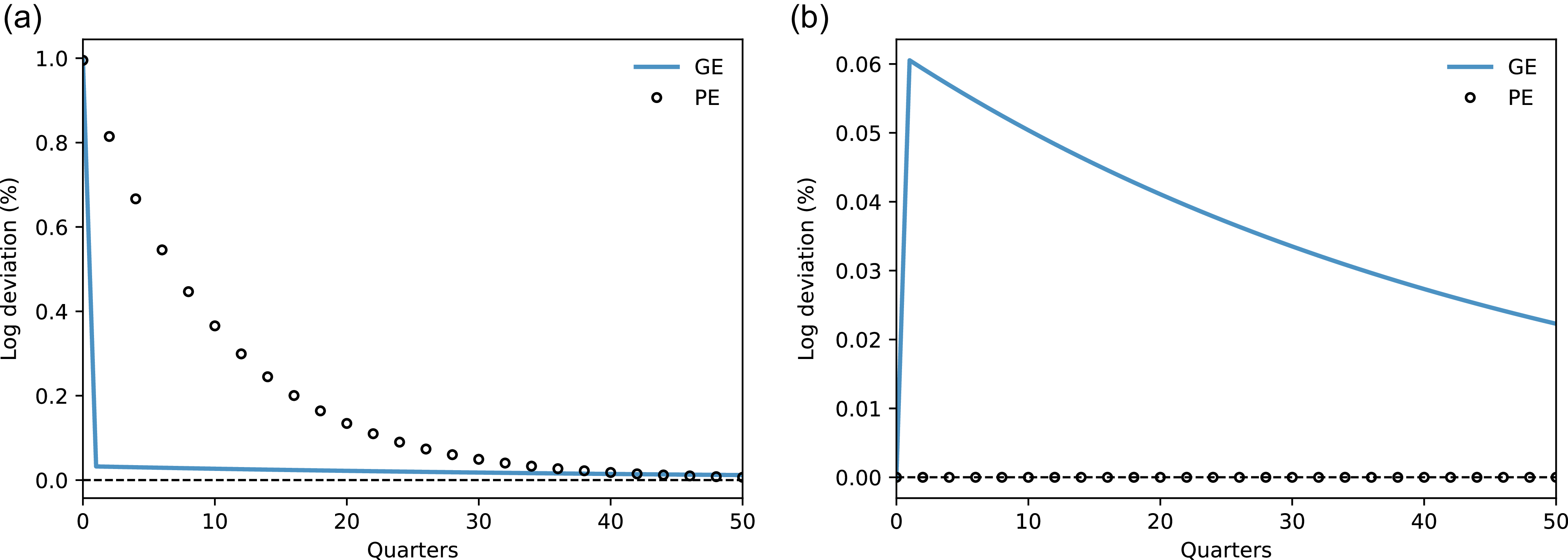
To illustrate the link between the GE solution (18)–(19) and the PE benchmark (20), Figure 1 plots the response of AI capacity and tangible capital to a one-off 1% increase in
 $M_t$
at date
 $0$
. The PE benchmark holds investment fixed at steady-state replacement levels and therefore abstracts from endogenous movements in consumption and marginal utility; it captures only passive depreciation-driven decay. The comparison measures how large the GE investment-adjustment feedbacks are in the baseline calibration. The solid lines show the GE impulse responses from the stable-manifold solution (Appendix B); the circle markers show the PE paths
 $m_t = (1-\delta _M)^t m_0$
and
 $k_t = 0$
(since only
 $M_0$
is shocked and PE investment in
 $K$
remains at replacement).
Adjustment after a 1% AI-capacity shock: GE vs. PE benchmark. Notes: The figure plots log deviations of
 $M_t$
(left panel) and
 $K_t$
(right panel) from the steady state following a 1% increase in
 $M_0$
. Solid lines: GE dynamics from the stable-manifold solution (Appendix B). Circle markers: PE benchmark, which holds investment at steady-state replacement levels so that deviations decay passively at the survival rate. The PE benchmark isolates depreciation-driven decay; the GE response allows investment to adjust, which closes stock gaps much faster for short-lived AI hardware because replacement flows are large relative to small deviations. For
 $K$
, the PE benchmark is zero by construction (only
 $M_0$
is shocked), whereas in GE the cross-effect through Cobb—Douglas production raises
 $K$
temporarily.

For AI capacity, the GE path adjusts markedly faster than the PE benchmark. The mechanism is straightforward: with
 $\delta _M\approx 0.095$
per quarter, steady-state replacement investment is about
 $9.5\%$
of the stock. A 1% excess stock is therefore small relative to replacement flows, so the planner can eliminate most of the deviation within a few quarters simply by cutting gross investment modestly below replacement while keeping
 $X_t\geq 0$
. The PE benchmark, which holds
 $X_t=\delta _M M^{*}$
by construction, captures only the passive component of this unwind and therefore decays more slowly, with a half-life of
 $t^{M}_{1/2}\approx 6.9$
quarters. For tangible capital, the PE benchmark is zero because only
 $M_0$
is shocked, but the GE path shows a temporary increase in
 $K$
driven by the cross-effect of higher AI capacity on the marginal product of tangible capital, followed by a slow return governed by the second eigenvalue.
6.4 Hardware-longevity shocks
Consider next a permanent reduction in the quarterly depreciation rate of AI capacity,
 $\delta _M \mapsto \delta _M - \Delta$
with
 $\Delta \gt 0$
, implemented at date
 $0$
. This shock shifts the steady state from
 $(K^{*},M^{*})$
to a new pair
 $(K^{**},M^{**})$
with higher AI capacity and higher tangible capital. In the GE system, the transition dynamics for the log deviations from the new steady state,
 $\tilde {k}_t \equiv \ln K_t - \ln K^{**}$
and
 $\tilde {m}_t \equiv \ln M_t - \ln M^{**}$
, again follow (18) with the Jacobian re-evaluated at
 $(K^{**},M^{**})$
.
As a transparent comparison, the PE benchmark assumes that the gap to the new AI steady state closes at the new survival rate:
 \begin{equation}M_t - M^{**} \approx (1-\delta _M + \Delta )^t\,\bigl (M_0 - M^{**}\bigr ).\end{equation}
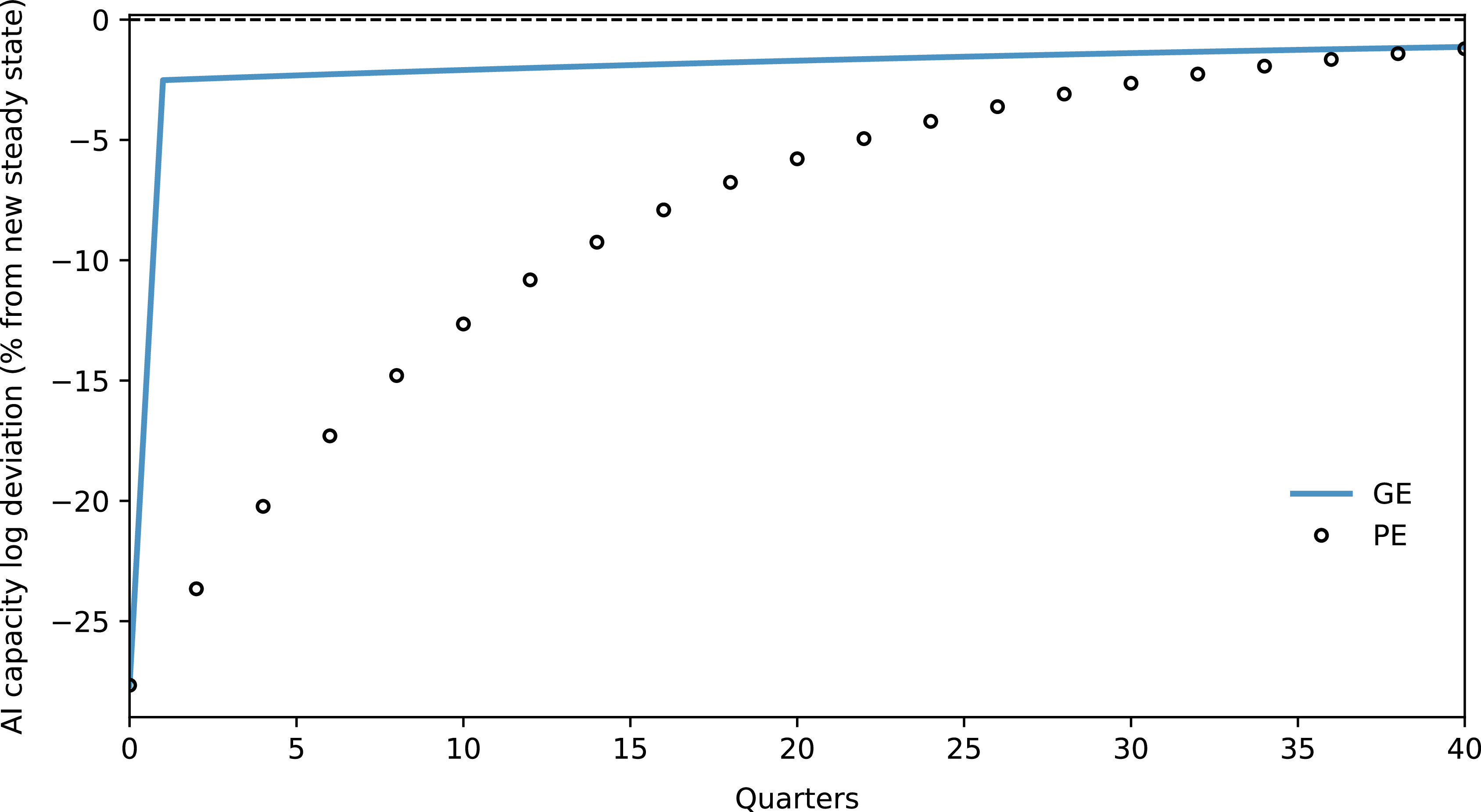
Figure 2 illustrates this transition for a two-percentage-point fall in the quarterly depreciation rate (from
 $\delta _M \approx 0.0953$
to
 $\delta _M - \Delta \approx 0.0753$
). As in Figure 1, the GE path adjusts faster than the PE benchmark because the planner re-optimises investment rather than holding it at replacement. The PE half-life of the gap to the new steady state is approximately
 \begin{equation*}t_{1/2}^{M,{\textrm{new}}} = {{\ln 0.5} \over {\ln (1 - {\delta _M} + \Delta )}} \approx 8.9\;{\textrm{quarters}},\end{equation*}
longer than in the baseline because the improvement in longevity slows adjustment.
Transition after a hardware-longevity improvement: GE vs. PE benchmark. Notes: The figure plots log deviations of AI capacity from the new steady state after a permanent two-percentage-point fall in
 $\delta _M$
. Solid line: GE dynamics re-evaluated at
 $(K^{**},M^{**})$
. Circle markers: PE benchmark (22), which holds investment at replacement levels so that the gap closes passively at the new survival rate
 $1-\delta _M+\Delta$
. The GE path adjusts faster because the planner front-loads AI investment in response to the permanent longevity improvement, exploiting the large replacement flows to close the gap to the new steady state more quickly.

6.5 Diffusion from a negligible initial stock
Finally, consider the adoption path of AI capacity when the economy starts from a negligible stock
 $M_0 \ll M^{*}$
. In the PE benchmark, applying the recursion with
 $M_0 \approx 0$
and constant investment at its steady-state value implies
 \begin{equation}M_t \approx M^{*}\left (1 - (1-\delta _M)^t\right ),\end{equation}
so that the gap to the steady state closes at the survival rate
 $1-\delta _M$
. With the baseline calibration, half of
 $M^{*}$
is reached after about
 $t^{M}_{1/2} \approx 6.9$
quarters and around 90% after roughly 23 quarters (just under six years).
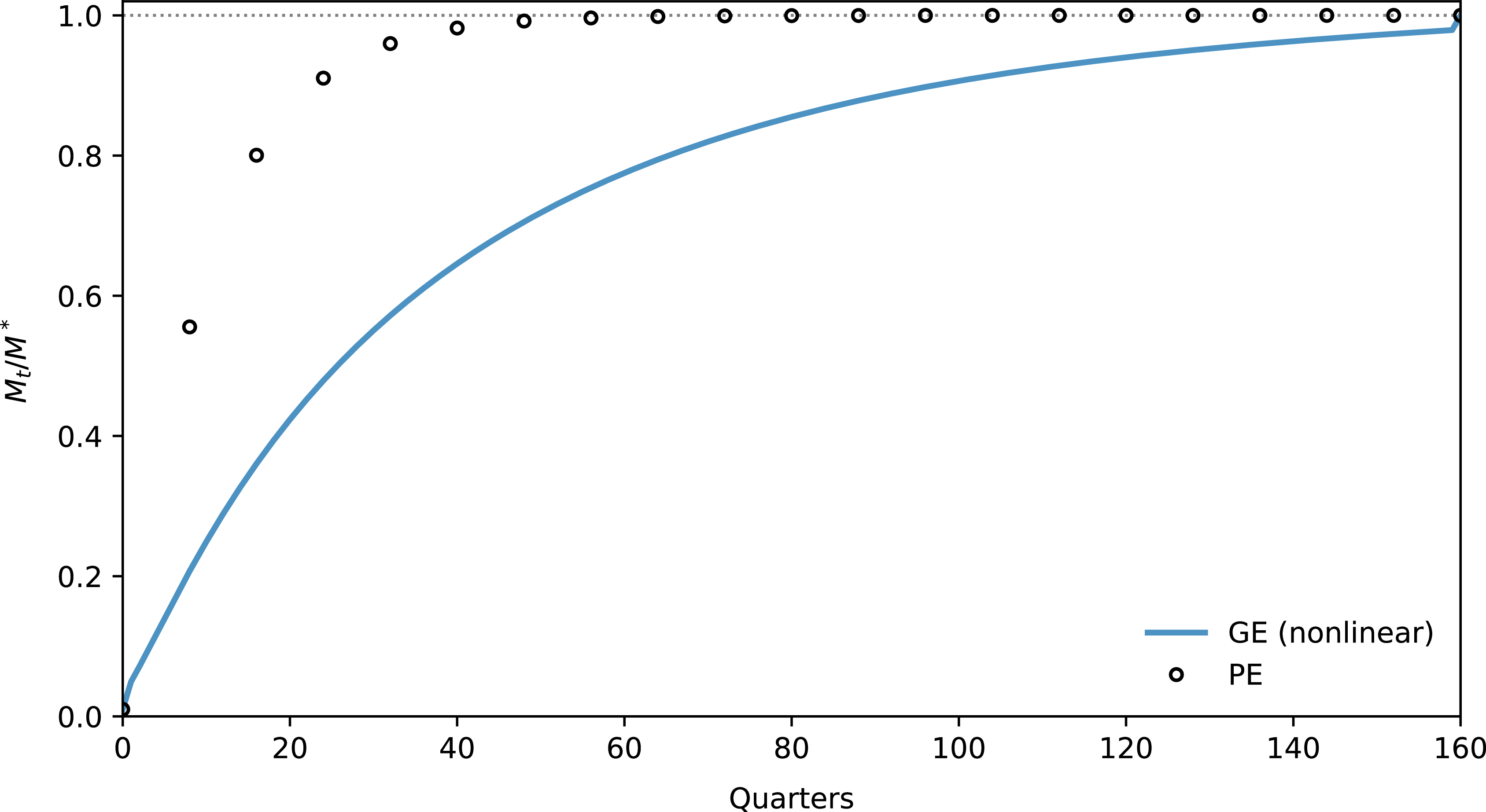
Unlike Figures 1 and 2, which are based on the local linear stable-manifold solution (19), the GE path in Figure 3 is computed from the nonlinear perfect-foresight system because the economy starts far from its steady state and a linear approximation would be unreliable. In the GE system, the qualitative pattern is similar but the speed of diffusion differs. Starting from a low
 $M_0$
and a correspondingly low
 $K_0$
, the planner must build up both capital stocks simultaneously while keeping consumption non-negative, which requires smoothing investment over a longer horizon than the PE benchmark assumes. As a result, the nonlinear perfect-foresight GE transition converges more slowly than (23): the PE benchmark implicitly front-loads investment at the steady-state replacement rate from date zero, whereas the GE planner optimally spreads the build-up across many periods. Figure 3 compares the two paths.
AI-capacity take-off from a low initial stock: GE vs. PE benchmark. Notes: The figure plots
 $M_t/M^{*}$
under a nonlinear perfect-foresight GE transition (solid line) and the PE diffusion benchmark (23) (circle markers) for an economy starting from
 $M_0 \approx 0$
. The PE benchmark holds investment fixed at steady-state replacement levels, implicitly front-loading capacity accumulation; the GE planner optimally smooths the build-up of both capital stocks, resulting in a more gradual diffusion path.

7. Policy experiments and measurement issues
The tractability of the framework means that many policy levers map into a small set of technology parameters, chiefly the effective depreciation rate of AI hardware and the marginal resource cost of inference,
 $\chi$
. Because the steady state is analytically characterised by two user—cost conditions (Section 4) and the linearised dynamics are governed by just two eigenvalues of the Jacobian
 $J$
(Section 6), a wide class of interventions can be evaluated with back-of-the-envelope expressions. For small shocks, the closed-form steady-state comparative statics in Appendix A and the geometric benchmarks from Section 6 provide very accurate approximations to the full general-equilibrium (GE) adjustment paths. Throughout this section we work with quarterly parameters. In particular,
 $\delta _M$
denotes the quarterly depreciation rate, and tax or longevity shocks are expressed in percentage points on this quarterly rate.
Compute taxation and accelerated depreciation
A tax on specialised hardware raises the user cost of AI capacity in exactly the same way as a higher depreciation rate. Let
 $\tau$
denote an ad-valorem tax on the purchase price of GPUs (or an equivalent surcharge on investment in
 $M_t$
), measured in percentage points on the quarterly rate. If firms write hardware off at the baseline
 $\delta _M$
, the effective depreciation rate becomes
 \begin{equation}\tilde \delta _M = \delta _M + \tau .\end{equation}
Policies that shorten the accounting life of hardware, add regulatory charges to data-centre assets, or impose a levy on compute all operate through this effective rate.
Let
 $M^*(\delta _M)$
denote the steady-state AI-capacity stock in the binding-capacity regime. Appendix A shows that
 $M^*$
is uniquely defined and strictly decreasing in
 $\delta _M$
. The semi-elasticity of steady-state capacity with respect to the hardware tax,
 \begin{equation*}\varepsilon _M^\tau \; \equiv \;{{\partial \ln {M^*}} \over {\partial \tau }} = {{\partial \ln {M^*}} \over {\partial {\delta _M}}},\end{equation*}
is therefore negative and can be computed directly from the implicit-function expression for
 $M^*$
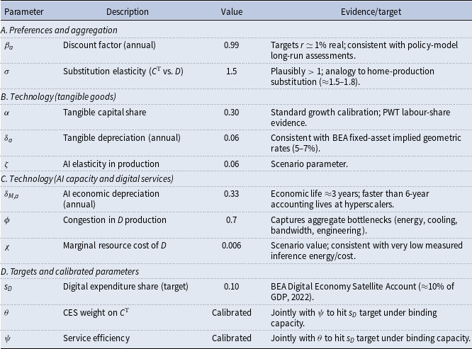
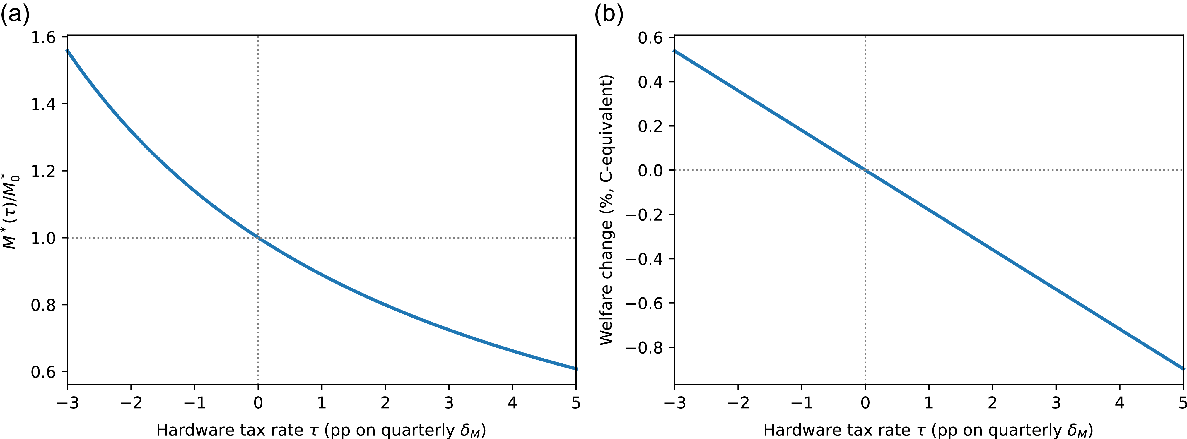
in Appendix A. In the baseline quarterly calibration (Table 1), this semi-elasticity is sizeable: a one-percentage-point surtax on hardware (
 $\tau =0.01$
) lowers the optimal AI-capacity stock by just over 10%, and a two-percentage-point surtax cuts it by about 20% (see panel (a) of Figure 4). Because the Cobb—Douglas exponents are fixed, the aggregate labour share
 $s^*_L=1-\alpha -\zeta$
remains unchanged; the tax acts purely on the scale of AI capital and on the distribution of capital income.
Baseline calibration (mid-2025)

Notes: Quarterly parameters used in the dynamics and policy analysis are
 $\beta =\beta _a^{1/4}\approx 0.9975$
,
 $\delta =1-(1-\delta _a)^{1/4}\approx 0.0154$
and
 $\delta _M=1-(1-\delta _{M,a})^{1/4}\approx 0.0953$
. All results in Sections 6 and 7 are computed in the binding-capacity steady state associated with this parameter vector.
Steady-state effects of a hardware tax (or subsidy). Notes: Panel (a) plots the ratio
 $M^*(\tau )/M^*_{0}$
as the effective hardware tax
 $\tau$
(in percentage points on the quarterly
 $\delta _M$
) varies. A two-percentage-point tax (
 $\tau =0.02$
) reduces the AI-capacity stock by approximately 20%. Panel (b) converts the utility change into consumption-equivalent units using (25). For moderate tax rates, welfare responds approximately linearly, with losses of around
 $0.18$
percentage points per percentage-point of tax.

The same logic applies in reverse to accelerated-depreciation allowances. Expensing an additional
 $\Delta$
of hardware, or introducing a targeted investment credit for AI-related equipment, is equivalent (in present-value terms) to
 $\tau =-\Delta$
in (24) and therefore raises
 $M^*$
with the same semi-elasticity. In this sense, standard hardware taxes and accelerated-depreciation policies can be viewed as symmetric instruments that move the effective depreciation rate in opposite directions. The transition towards the new steady state is dominated by the fast GE eigenvalue
 $\lambda _1$
(Section 6), so the resulting adjustment in
 $M_t$
unfolds over a horizon of only a few years.
Permanent hardware-longevity shock
A once-and-for-all reduction in the economic depreciation rate of AI hardware,
 $\delta _M\mapsto \delta _M-\Delta$
with
 $\Delta \gt 0$
, captures improvements in hardware design, repairability, or cooling that extend the useful life of GPUs and related infrastructure. Linearising the steady-state condition for
 $M^*$
with respect to
 $\delta _M$
and aggregating the consumption stream along the transition path yields a closed-form welfare gain, expressed in consumption-equivalent units:
 \begin{equation}\Omega (\Delta ) = {{\beta (1 - \beta ){\mkern 1mu} \Delta } \over {(1 - \beta + \beta {\mkern 1mu} {\delta _M})(1 - \phi )}}{\mkern 1mu} {{{M^*}} \over {{C^*}}},\end{equation}
where
 $C^*$
is steady-state consumption and
 $(\beta ,\delta _M,\phi )$
are the quarterly parameters (with
 $\beta =\beta _a^{1/4}$
).Footnote
11
For the baseline calibration (implying quarterly
 $\beta \approx 0.9975$
and
 $\delta _M\approx 0.0953$
, with
 $\phi =0.7$
), the coefficient in front of
 $M^*/C^*$
in (25) is approximately
 $0.086$
. Given the baseline steady-state ratio
 $M^*/C^* \approx 2.1$
, this implies
 \begin{equation*}\Omega (\Delta )\;\approx \;0.18\,\Delta . \end{equation*}
A two-percentage-point improvement in hardware longevity on the quarterly rate (
 $\Delta =0.02$
) therefore raises lifetime utility by roughly
 $0.36$
% in consumption-equivalent terms (see panel (b) of Figure 4). Because the transition in
 $M_t$
is governed by the fast adjustment mode, a substantial fraction of this gain accrues in the first few years: under the PE passive-decay yardstick the bulk of the adjustment in AI capacity is complete within roughly two half-lives (about three to four years), and the GE system can be materially faster, after which the economy is close to its new steady state.
Competition policy
Dominant cloud providers often enjoy contractual and scale advantages that lower their private effective depreciation rate: bespoke maintenance contracts, favourable power-purchase agreements, or proprietary cooling solutions all allow hardware to remain in service longer than for a marginal entrant. Reversing part of that asymmetry, through data-portability mandates, interoperability standards, or limits on exclusive service contracts, can be viewed as a policy that raises the incumbent’s effective
 $\delta _M$
towards the economy-wide baseline.
Within the present framework, any such intervention operates through the same
 $M^*(\delta _M)$
schedule as a hardware tax. Using the semi-elasticity discussed above, a five-percentage-point increase in an incumbent’s effective quarterly depreciation rate would, in the baseline calibration, reduce its optimal capacity stock by on the order of
 $40$
%. Because digital services are produced at very low marginal resource cost once capacity is installed, the welfare cost of a moderate reduction in scale is second order, whereas the potential pro-competitive gains lie largely outside the representative-agent model.
Macroprudential timing
The high depreciation rate of AI hardware also has implications for financial-stability tools. Suppose hardware investment is partly debt-financed and that policymakers wish to lean against AI-driven credit booms by introducing a counter-cyclical capital buffer. The PE passive-decay benchmark provides a conservative guide to the speed at which hardware-driven booms unwind once investment returns to replacement:
 \begin{equation*}t_{1/2}^{{\textrm{PE}}} = {{\ln 0.5} \over {\ln (1 - {\delta _M})}} \approx 6.9\;{\textrm{quarters}},\end{equation*}
or roughly one and three-quarter years in the baseline calibration. As Figures 1–2 illustrate, the GE adjustment can be substantially faster because the planner (or market participants) can cut gross investment below replacement, exploiting the large steady-state replacement flows that characterise short-lived assets. A simple prudential rule that accumulates capital buffers during hardware-investment booms and releases them on a schedule tied to the PE half-life would therefore provide a transparent and conservative timing benchmark. Unlike traditional Basel III buffers, which often release with multi-year lags, such a rule can be calibrated ex ante from observable hardware depreciation rates and replacement cycles, making it both transparent and time-consistent.
8. Extensions and robustness
The two-asset core explains how hardware longevity, inference cost, and substitution elasticities shape growth and factor incomes once AI capacity is part of the production process. This section sketches three modifications that preserve the algebraic backbone of the model while opening avenues for distributional and monetary analysis. In each case, the
 $\{K_t,M_t\}$
block, its steady-state characterisation and its linear general-equilibrium (GE) dynamics remain exactly as in Sections 4–6; the extensions either add margins that are analytically separable or enter through static wedges in wage-setting or price-setting conditions. The eigenvalues of the core two-asset system, and the associated GE and PE dynamics, are therefore unchanged.
8.1 Heterogeneous labour and wage polarisation
Let labour consist of routine and non-routine types,
 $L^{\textrm R}_t$
and
 $L^{\textrm N}_t$
, aggregated with elasticity
 $\nu \gt 1$
:
 \begin{equation*}{Y_t} = AK_t^\alpha M_t^\zeta {\left[(1 - \omega )L_t^{\textrm{N}} + \omega {(\xi {M_t}L_t^{\textrm{R}})^{(\nu - 1)/\nu }}\right]^{{\nu \over {\nu - 1}}(1 - \alpha - \zeta )}}.\end{equation*}
AI capacity is assumed to substitute more strongly for routine tasks; the parameter
 $\xi \gt 0$
scales that substitutability. Because each labour type supplies perfect substitutes within its own class, the wage ratio is pinned down in closed form:
 \begin{equation*}{{w_t^{\textrm{N}}} \over {w_t^{\textrm{R}}}} = {(\xi {M_t})^{{{\nu - 1} \over \nu }}}.\end{equation*}
Choosing
 $(\nu ,\xi )=(1.08,1)$
implies that a doubling of
 $M_t$
widens the non-routine wage premium by
 $2^{(\nu -1)/\nu }\approx 1.053$
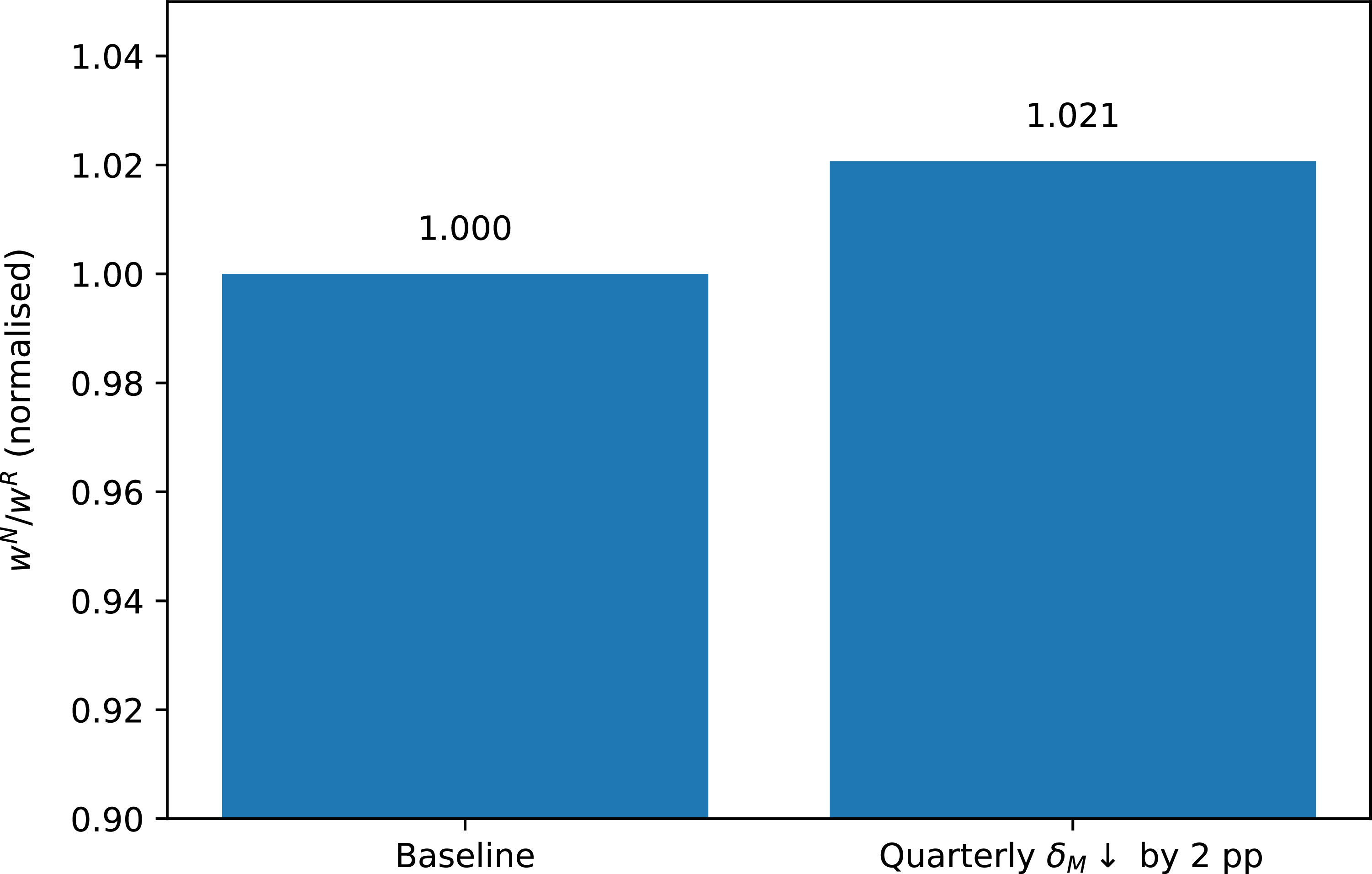
, i.e. just over 5%. This magnitude is consistent with the rise in the EU Structure of Earnings Survey between 2018 and 2022 for tasks classified as “information-processing” versus “manual”. In the baseline calibration, the two-percentage-point longevity improvement in Section 7 raises steady-state stock of AI capacity by roughly one third, which implies a wage premium of about 2%, as shown in Figure 5.Footnote
12
Wage premium after hardware-longevity shock. Notes: Bars display the wage ratio
 $w^{\textrm N}/w^{\textrm R}$
in the baseline steady state (left) and after a permanent two-percentage-point fall in the quarterly depreciation rate
 $\delta _M$
(right). For the parameter choice
 $(\nu ,\xi )=(1.08,1)$
, the new steady state exhibits a wage premium of just over 2%, consistent with the log-elasticity
 $\partial \ln (w^{\textrm N}/w^{\textrm R})/\partial \ln M = (\nu -1)/\nu \approx 0.074$
.

This extension preserves analytical tractability. The capital block remains two-dimensional, and the wage ratio follows directly from
 $M_t$
without introducing additional state variables. Shocks that raise steady-state AI capacity, such as the hardware-longevity improvements in Section 7, therefore translate one-for-one into predictable changes in skill premia, with the speed of adjustment governed by the fast eigenvalue of the
 $\{K_t,M_t\}$
system.
8.2 Nominal rigidities and inflation dynamics
Embedding the consumption-side CES aggregator in a Dixit—Stiglitz price-setting framework preserves the log-linearity of the Euler block. Suppose a continuum of differentiated firms sets prices à la Calvo, with probability
 $1-\rho$
of resetting in any given period. Linearising the New Keynesian Phillips curve around the AI-augmented steady state yields
 \begin{equation}{\pi _t} = \beta {\mkern 1mu} {_t}{\pi _{t + 1}} + \kappa {\mkern 1mu} {\hat u_t},\qquad \kappa = {{(1 - \rho )(1 - \beta \rho )} \over \rho }{\mkern 1mu} {{1 - \theta } \over {\theta \sigma }},\end{equation}
where
 $\hat {u}_t$
is the log deviation of real marginal cost from its flexible-price level, and
 $\beta$
is the quarterly discount factor. In the present environment, real marginal cost is tied to the tangible-goods price and the CES weight on digital services, so
 $\hat {u}_t$
becomes a linear function of hardware costs and of the relative price of digital consumption.
A surprise improvement in hardware longevity, modelled as a fall in
 $\delta _M$
, therefore acts as a sequence of negative cost-push shocks. In the binding-capacity regime, the impact on
 $\hat {u}_t$
is approximately proportional to the change in the effective user cost of AI capacity. With
 $\rho =0.75$
(implying an average price duration of one year) and the baseline calibration in Section 5, a four-percentage-point reduction in quarterly
 $\delta _M$
generates an initial disinflation of roughly
 $0.3$
percentage points on a year-on-year basis, with the effect decaying over about three quarters. The exact paths follow directly from (26) once one specifies a monetary-policy rule and feeds in the
 $\{K_t,M_t\}$
path from the core GE system.
8.3 Endogenous model size
Thus far, the stock of AI capacity
 $M_t$
captures only hardware and associated infrastructure. To allow for endogenous model size, let
 $S_t$
denote the number of parameters (or an effective complexity index) of the frontier model. The capacity constraint for digital services becomes
 \begin{equation*}D_t \;\le \; \psi \,M_t^{\phi } S_t^{\vartheta },\qquad 0\lt \vartheta \lt 1, \end{equation*}
so that, under binding capacity,
 $D_t=\psi \,M_t^{\phi } S_t^{\vartheta }$
. The new state variable
 $S_t$
evolves according to
 \begin{equation*}S_{t+1}=(1-\delta _S)S_t+I^S_t, \end{equation*}
with
 $\delta _S\in (0,1)$
capturing obsolescence from data staleness and architectural advances, and
 $I^S_t$
denoting “training investment” (engineering and compute devoted to growing the model).
Because
 $S_t$
does not enter tangible-goods production
 $Y_t$
, the
 $\{K_t, M_t\}$
block is determined independently of
 $S_t$
. The system is recursive: once
 $(K^{*}, M^{*})$
are pinned down, the Euler equation for
 $S_t$
determines
 $S^{*}$
conditional on that block. In the binding-capacity regime, the steady-state Euler condition for
 $S^{*}$
takes the form
 \begin{equation}1 = \beta \big [(1-\delta _S) + \big (MRS^{*} - \chi \big )\,\vartheta \,\psi \,(M^{*})^{\varphi } (S^{*})^{\vartheta -1}\big ],\end{equation}
with
 $MRS^{*}$
defined as in Section 4. The right-hand side of (27) is strictly decreasing in
 $S^{*}$
, guaranteeing a unique interior solution for the training stock. A permanent fall in
 $\delta _S$
raises
 $S^{*}$
while leaving
 $M^{*}$
and the Jacobian of the
 $\{K_t, M_t\}$
subsystem essentially unchanged: training and inference respond on separate margins, and the two GE eigenvalues for the hardware block are preserved.
9. Conclusion
This paper has developed a simple two-asset growth model in which AI capacity joins conventional capital as a separate reproducible asset. AI capacity is interpreted as installed, rival hardware and infrastructure that embody non-rival models, deliver low-marginal-cost digital services, and raise productivity in the tangible-goods sector. The steady state of this economy is analytically characterised by two user-cost conditions: one pins down a power-law relationship between tangible capital and AI capacity, the other determines the unique interior AI stock as the root of a monotone marginal-benefit map. Linearising around this steady state yields a two-dimensional general-equilibrium (GE) system with two eigenvalues whose stable manifold defines a two-dimensional law of motion for the capital stocks. Simple geometric laws of motion based on the survival rates provide transparent PE benchmarks for policy experiments.
Three quantitative lessons emerge. First, hardware durability is the dominant state variable. It governs the PE passive-decay half-life of AI-investment booms (roughly seven quarters in the baseline calibration), dictates how much capacity firms wish to hold, and controls the size of the digital block. Because replacement flows are large for short-lived assets, the GE planner can close small stock gaps substantially faster than passive decay; conversely, conventional capital adjusts over more than a decade. Second, the elasticity with which digital services substitute for tangible consumption, together with the marginal resource cost of inference, acts as the key wedge between growth and measured inflation: when the marginal cost of inference is very low, modest changes in these parameters can generate large shifts in expenditure shares with only small movements in aggregate output. Third, because the aggregate labour share is pinned down by primitive Cobb—Douglas exponents, most redistribution in the baseline model runs through capital ownership rather than through wages, unless AI is allowed to substitute directly for particular labour types in production.
In the baseline calibration, a one-percentage-point hardware tax on the quarterly depreciation rate reduces the optimal AI capacity stock by just over 10%, while a two-percentage-point tax cuts it by about 20%. Conversely, an equally sized extension of GPU service lives, interpreted as a two-percentage-point fall in the quarterly economic depreciation rate, raises lifetime welfare by around
 $0.36$
% in consumption-equivalent terms. The same primitives govern prudential timing: the PE passive-decay benchmark implies that AI-investment booms unwind with a half-life of about seven quarters once investment returns to replacement, and the GE adjustment can be faster still, so a counter-cyclical capital buffer aimed at AI lending can be released within roughly two years of an investment peak without elaborate forecasting. Overall, the framework points to hardware-centric instruments (accelerated depreciation, compute levies, repair mandates) as levers with unusually high marginal bite, and quantifies their effects using transparent steady-state elasticities and simple dynamic adjustments.
Several avenues remain open. Endogenising the training stock allows model size to interact with hardware cycles; layering on heterogeneous labour maps capacity growth into earnings dispersion; and introducing nominal rigidities turns hardware shocks into measurable disinflation episodes. None of these extensions threatens tractability: they either add separable state variables or introduce static wedges, leaving the two-asset core, its user-cost characterisation, and its GE eigenvalues intact. What they do require is better empirical measurement of three quantities: effective GPU depreciation, the true marginal resource cost of inference (including energy and cooling), and the substitution elasticities between digital and tangible uses (in both consumption and production). Improving those measurements is likely to deliver a higher marginal return than rerunning ever more elaborate simulations on poorly pinned-down parameters.
The central point is straightforward. Assets that depreciate quickly behave differently from assets that last. When AI hardware depreciates at more than 30% per year, the horizon for policy intervention shrinks from decades to years, and the fiscal cost of poorly timed incentives compounds just as fast. A framework that keeps the arithmetic in the foreground provides a useful starting point for thinking about the macroeconomics of the next wave of capital deepening.
A. Existence and uniqueness of the steady state
This appendix provides a rigorous proof of existence, uniqueness, and interiority of the steady state. The analysis is conducted for a generalised Euler-return map that nests both the slack- and binding-capacity regimes implied by the Kuhn—Tucker conditions and underpins the steady-state characterisation in Section 4. All arguments are purely static and do not depend on the linearised dynamics in Section 6.
A.1. Feasible domain and primitives
Throughout the appendix we impose the baseline assumptions from Section 3, and we make explicit the parameter restrictions used below:
 \begin{equation*}\alpha \in (0,1),\!\quad\! \beta \in (0,1),\!\!\quad 0\lt \zeta \lt 1-\alpha ,\!\!\quad \phi \in (0,1],\!\!\quad \psi \gt 0,\!\quad \delta _M\ge 0,\!\!\quad \delta \in [0,1),\!\!\quad A\gt 0,\!\!\quad \chi \ge 0, \end{equation*}
and (for the CES subutility)
 $\theta \in (0,1)$
and
 $\sigma \gt 0$
. To match the baseline specification in Sections 3–5, we adopt the CES aggregator with the weight on tangible consumption, where
 $C_T$
corresponds to
 $C^{\textrm T}$
in the main text:
 \begin{equation*}U({C_T},D) = {\left[\theta {\mkern 1mu} C_T^\rho + (1 - \theta ){\mkern 1mu} {D^\rho }\right]^{1/\rho }},\qquad \rho \equiv {{\sigma - 1} \over \sigma },\end{equation*}
with the case
 $\sigma =1$
understood in the CES limit
 $\rho \to 0$
; the expressions below remain valid in that limit (all limits are well-behaved as
 $\sigma \to 1$
). Hence the marginal rate of substitution of
 $D$
for
 $C_T$
, which is also the shadow price of digital services in units of tangible consumption, is
 \begin{equation*}{p_D}\; \equiv \;{\textrm{MRS}}({C_T},D)={{{U_D}} \over {{U_{{C_T}}}}}={{1 - \theta } \over \theta }{\left( {{{{C_T}} \over D}} \right)^{1/\sigma }}.\end{equation*}
The CES subutility is strictly increasing and concave for all
 $\sigma \gt 0$
and
 $\theta \in (0,1)$
.
Feasible allocations require
 $C_T\gt 0$
and
 $D\ge 0$
.
Steady-state ratios and power-law relationships
The tangible-capital Euler condition implies a steady-state output—capital ratio:
 \begin{equation*}{\Lambda _K}\; \equiv \;{{{\beta ^{ - 1}} - (1 - \delta )} \over \alpha }\;{\gt}\;0,\qquad \Rightarrow \qquad {{{Y^*}} \over {{K^*}}} = {\Lambda _K}.\end{equation*}
Combining
 $Y^*=\Lambda _K K^*$
with
 $Y^*=A (K^*)^{\alpha } M^{\zeta }$
yields power-law relationships in
 $M$
:
 \begin{equation*}{K^*}(M) = {\kappa _K}{\mkern 1mu} {M^\gamma },\qquad {Y^*}(M) = {\kappa _Y}{\mkern 1mu} {M^\gamma },\qquad \gamma \; \equiv \;{\zeta \over {{\mkern 1mu} 1 - \alpha {\mkern 1mu} }} \in (0,1),\end{equation*}
where
 $\kappa _K\equiv (A/\Lambda _K)^{1/(1-\alpha )}$
and
 $\kappa _Y\equiv \Lambda _K\,\kappa _K$
. Note that
 \begin{equation*}{\kappa _Y} - \delta {\kappa _K} = {\kappa _K}({\Lambda _K} - \delta ),\qquad {\Lambda _K} - \delta = {{{\beta ^{ - 1}} - 1 + \delta (1 - \alpha )} \over \alpha }{\gt}0,\end{equation*}
so
 $\kappa _Y-\delta \kappa _K\gt 0$
.
Capacity and the at-capacity MRS
Capacity for digital services is
 \begin{equation*}D^{\textrm{cap}}(M)=\psi \,M^{\phi }. \end{equation*}
The (counterfactual) MRS of
 $D$
for
 $C_T$
evaluated at capacity is
 \begin{equation*}p_D^{{\textrm{cap}}}(M) = {{1 - \theta } \over \theta }{\left( {{{C_T^{{\textrm{cap}}}(M)} \over {{D^{{\textrm{cap}}}}(M)}}} \right)^{1/\sigma }},\end{equation*}
where the tangible-goods resource constraint at capacity is
 \begin{equation}C_T^{\textrm{cap}}(M) = Y^*(M) - \delta K^*(M) - \delta _M M - \chi D^{\textrm{cap}}(M) = \bigl (\kappa _Y-\delta \kappa _K\bigr ) M^\gamma - \delta _M M - \chi \psi \,M^{\phi }.\end{equation}
In the binding regime the optimum saturates capacity, so
 $D^*=D^{\textrm{cap}}$
and
 $p_D^*\ge \chi$
(with strict inequality if and only if the capacity multiplier is strictly positive,
 $\eta \gt 0$
); in the slack regime the planner chooses
 $D^*\lt D^{\textrm{cap}}$
so that
 $p_D^*=\chi$
.
Assumption A.1. (Feasibility near the origin)
 \begin{equation*}\phi \;\ge \; \gamma \quad \text{and, if }\phi =\gamma ,\text{ then }\; \kappa _Y-\delta \kappa _K \;\gt \; \chi \psi . \end{equation*}
Assumption A.1 ensures
 $C_T^{\textrm{cap}}(M)\gt 0$
for sufficiently small
 $M\gt 0$
: near
 $M=0$
,
 $M^\gamma$
dominates
 $M$
because
 $M^{\gamma }/M=M^{\gamma -1}\to \infty$
since
 $\gamma \in (0,1)$
. Requiring
 $\phi \ge \gamma$
ensures that the resources required for capacity, which scale with
 $M^\phi$
, vanish weakly faster than output near the origin (i.e.
 $M^\phi /M^\gamma \to 0$
when
 $\phi \gt \gamma$
); if
 $\phi =\gamma$
we impose a strictly positive coefficient.
Economic intuition. Assumption A.1 guarantees that, when the stock
 $M$
is very small, the resource needs for capacity (
 $\chi \psi M^\phi$
) and for maintenance (
 $\delta _M M$
) do not exceed the net output available to tangible consumption
 $(\kappa _Y-\delta \kappa _K)M^\gamma$
. This ensures the economy is viable near the origin.
Boundary of the feasible set
We use the at-capacity resource constraint to define a conservative feasibility domain on which
 $p_D^{\textrm{cap}}(M)$
and the generalised map are well-defined on
 $\mathcal D$
:
 \begin{equation*}M_{\max }\;\equiv \; \sup \{M\gt 0:\ C_T^{\textrm{cap}}(M)\gt 0\}\ \in \ (0,\infty ], \qquad \mathcal D\;\equiv \; (0,M_{\max }). \end{equation*}
On
 $\mathcal D$
,
 $C_T^{\textrm{cap}}(M)\gt 0$
and
 $D^{\textrm{cap}}(M)\gt 0$
, so
 $C_T^{\textrm{cap}}(M)/D^{\textrm{cap}}(M)\gt 0$
and hence
 $p_D^{\textrm{cap}}(M)$
is well-defined. Since
 $C_T^{\textrm{cap}}(\cdot )$
is continuous in
 $M$
, the boundary property below follows. By Assumption A.1 the set
 $\{M\gt 0:\,C_T^{\textrm{cap}}(M)\gt 0\}$
is nonempty and open near
 $M=0$
, so
 $\mathcal D=(0,M_{\max })\neq \varnothing$
. This domain is sufficient for feasibility under binding capacity; if capacity is slack, feasibility may also obtain for larger
 $M$
with
 $D^*\lt D^{\textrm{cap}}$
, but the generalised map below is constructed on
 $\mathcal D$
(and Proposition 1 shows that no steady state exists with
 $M\ge M_{\max }$
anyway).
Lemma 1 (Characterisation of
 $M_{\max }$
). Under Assumption A.1 there exists a unique
 $M_{\max }\in (0),\infty ]$
such that
 $C_T^{\textrm{cap}}(M)\gt 0$
for all
 $M\in (0,M_{\max })$
and, if
 $M_{\max }\lt \infty$
, then
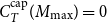 $C_T^{\textrm{cap}}(M_{\max })=0$
.
Roadmap. We study the intersection of
 $L(M)\equiv (\kappa _Y-\delta \kappa _K)-\chi \psi \,M^{\phi -\gamma }$
and
 $R(M)\equiv \delta _M M^{1-\gamma }$
. The behaviour of
 $L$
depends on whether
 $\phi \gt \gamma$
(decreasing when
 $\chi \gt 0$
, constant when
 $\chi =0$
) or
 $\phi =\gamma$
(constant);
 $R$
is strictly increasing when
 $\delta _M\gt 0$
and identically zero when
 $\delta _M=0$
. This yields uniqueness (or
 $M_{\max }=+\infty$
) case by case.
Proof.
Setting
 $C_T^{\textrm{cap}}(M)=0$
in (1) and dividing both sides by
 $M^\gamma$
(valid for
 $M\gt 0$
), we obtain
 \begin{equation*}(\kappa _Y-\delta \kappa _K) \;-\; \chi \psi \,M^{\phi -\gamma } = \delta _M M^{1-\gamma }. \end{equation*}
Let
 $L(M)\equiv (\kappa _Y-\delta \kappa _K)-\chi \psi \,M^{\phi -\gamma }$
and
 $R(M)\equiv \delta _M M^{1-\gamma }$
. Since
 $1-\gamma \gt 0$
,
 $R(M)$
is continuous and (strictly) increasing on
 $(0,\infty )$
when
 $\delta _M\gt 0$
, and
 $R(M)\equiv 0$
when
 $\delta _M=0$
.
-
• If
 $\phi \gt \gamma$
, then when
$\chi \gt 0$
the function
$L(M)$
is strictly decreasing from
$L(0^+)=(\kappa _Y-\delta \kappa _K)\gt 0$
to
$-\infty$
; if
$\chi =0$
, then
$L(M)\equiv (\kappa _Y-\delta \kappa _K)\gt 0$
is constant.
-
− If
$\delta _M\gt 0$
,
$L$
and
$R$
intersect once at some finite
$M_{\max }$
. -
− If
$\delta _M=0$
and
$\chi \gt 0$
, the unique finite
$M_{\max }$
solves
$L(M_{\max })=0$
(when
$\phi \gt \gamma$
). -
− If
$\delta _M=0$
and
$\chi =0$
, then
$L(M)\equiv (\kappa _Y-\delta \kappa _K)\gt 0$
and
$R(M)\equiv 0$
, so
$C_T^{\textrm{cap}}(M)\gt 0$
for all
$M$
and
$M_{\max }=+\infty$
.
-
-
• If
$\phi =\gamma$
, then
$L(M)\equiv (\kappa _Y-\delta \kappa _K-\chi \psi )\gt 0$
by Assumption A.1.-
− If
$\delta _M\gt 0$
, there is a unique finite solution
$M_{\max }\gt 0$
to
$L(M_{\max })=R(M_{\max })$
. -
− If
$\delta _M=0$
, the equality has no finite solution and
$M_{\max }=+\infty$
.
-

















Summary:
 $M_{\max }=+\infty$
if and only if
 $\delta _M=0$
and either (A)
 $\phi =\gamma$
or (B)
 $\phi \gt \gamma$
with
 $\chi =0$
. Otherwise
 $M_{\max }\in (0,\infty )$
,unique.
A.2. Prices, regimes, and the generalised Euler-return map
The Kuhn—Tucker conditions imply two regimes. In the binding regime, capacity saturates so
 $D^*=\psi M^{\phi }$
and
 $p_D^*\ge \chi$
(with strict inequality if and only if
 $\eta \gt 0$
); in the slack regime the planner sets
 $p_D^*=\chi$
by choosing
 $D^*\lt D^{\textrm{cap}}$
.
We set the Lagrange multiplier on the tangible resource constraint to
 $\lambda =U_{C_T}$
and measure prices in
 $C_T$
units by dividing all FOCs by
 $U_{C_T}$
; equivalently, we take
 $C_T$
as the numeraire. Let
 $\tilde \eta (M)\ge 0$
denote the raw multiplier on the capacity constraint
 $D\le \psi M^\phi$
, and define the (numeraire-)normalised capacity multiplier
 $\eta (M)\equiv \tilde \eta (M)/U_{C_T}$
so that all multipliers are in
 $C_T$
units. The
 $D$
-stationarity condition is
 \begin{equation*}p_D-\chi -\eta =0,\qquad \eta \ge 0,\qquad \eta \bigl (\psi M^\phi -D\bigr )=0. \end{equation*}
Evaluating at capacity implies
 \begin{equation*}\eta (M)=\max \{0,\,p_D^{\textrm{cap}}(M)-\chi \}. \end{equation*}
In the slack regime,
 $p_D^*=\chi$
at the optimal
 $D^*\lt D^{\textrm{cap}}$
. Increasing
 $D$
toward capacity raises
 $D$
and lowers
 $C_T$
, thereby reducing the MRS under CES preferences; hence
 $p_D^{\textrm{cap}}(M)\le \chi$
whenever the capacity constraint is slack. Within period
 $t$
, the stocks
 $K_t$
and
 $M_t$
are predetermined.
Generalised Euler return
 \begin{align} G(M) &\equiv \left( {1 - {\delta_{M}}} \right) + \zeta {{{Y^*}(M)} \over M} + \eta (M)\phi \psi {M^{\phi - 1}} \notag\\ &=\left( {1 - {\delta_{M}}} \right) + \zeta {{{Y^*}(M)} \over M} + \max \left\{ {0,p_D^{{\textrm{cap}}}(M) - \chi } \right\}\phi \psi {M^{\phi - 1}},\quad M \in {\phi ^2},\end{align}
We refer to
 $G$
as the generalised Euler return. Economically, the first two terms are the standard gross return on
 $M$
; we refer to the third term in (2) as the services dividend, which is present only when capacity binds.
Equivalently, resolving the max by regime,
 \begin{equation*}G(M) = \left\{{\begin{matrix}(1 - {\delta _M}) + \zeta {\mkern 1mu} {{{Y^*}(M)} \over M} +(p_D^{{\textrm{cap}}}(M) - \chi ){\mkern 1mu} \phi \psi {\mkern 1mu} {M^{\phi - 1}}, &\quad{\textrm{if }}p_D^{{\textrm{cap}}}(M){\gt}\chi , \\[6pt](1 - {\delta _M}) + \zeta {\mkern 1mu} {{{Y^*}(M)} \over M}, &\quad{\textrm{if }}p_D^{{\textrm{cap}}}(M) \le \chi.\end{matrix}}\right.\end{equation*}
We analyse
 $G$
on
 $\mathcal D=(0,M_{\max })$
. In steady state, the Euler condition for
 $M$
is
 \begin{equation}1 = \beta \,G(M^*).\end{equation}
Note on the productivity term: because
 $K$
is predetermined within the period, the envelope/Euler return uses the partial marginal product holding
 $K$
fixed,
 $\partial Y/\partial M=\zeta \,Y/M$
for Cobb—Douglas
 $Y=A K^\alpha M^\zeta$
. We then evaluate at the steady-state allocation
 $K^*(M)$
for notational convenience.
Lemma 2. (Monotonicity and continuity of
 $G$
). Under Assumption A.1, on
 $\mathcal D=(0,M_{\max })$
the map
 $G(\!\cdot\! )$
is continuous and strictly decreasing. The at-capacity MRS
 $p_D^{\textrm{cap}}(M)$
is (weakly) decreasing in
 $M$
and is constant on
 $\mathcal D$
if and only if
 $\delta _M=0$
and
 $\phi =\gamma$
; equivalently,
 $p_D^{\textrm{cap}}$
is strictly decreasing unless this knife-edge holds. Moreover, at any
 $M$
with
 $p_D^{\textrm{cap}}(M)=\chi$
, the services term is zero on the slack side and tends to zero from the binding side, hence
 $G$
is continuous (though generally not differentiable) at the endogenous regime boundary. Because
 $G$
is strictly decreasing on
 $\mathcal D$
, it is injective.
Proof. We analyse each component of (2).
-
(i) Productivity term. Since
$Y^*(M)=\kappa _Y M^\gamma$
with
$\gamma \in (0,1)$
,
$\zeta \,Y^*(M)/M=\zeta \kappa _Y M^{\gamma -1}$
is strictly decreasing in
$M$
. -
(ii) At-capacity MRS monotonicity. Using (1) and
$D^{\textrm{cap}}=\psi M^\phi$
, first divide by
$D^{\textrm{cap}}$
:with
\begin{equation*}{{C_T^{{\textrm{cap}}}} \over {{D^{{\textrm{cap}}}}}} = {{{\kappa _Y} - \delta {\kappa _K}} \over \psi }{\mkern 1mu} {M^{\gamma - \phi }}\; - \;{{{\delta _M}} \over \psi }{\mkern 1mu} {M^{1 - \phi }}\; - \;\chi = {c_1}{M^{\gamma - \phi }} - {c_2}{M^{1 - \phi }} - \chi ,\end{equation*}
${c_1} = {{{\kappa _Y} - \delta {\kappa _K}} \over \psi }{\gt}0$
and
${c_2} = {{{\delta _M}} \over \psi } \ge 0$
. Differentiating givesbecause
\begin{equation*}{d \over {dM}}\left({{C_T^{{\textrm{cap}}}} \over {{D^{{\textrm{cap}}}}}}\right) = {c_1}(\gamma - \phi ){M^{\gamma - \phi - 1}} - {c_2}(1 - \phi ){M^{ - \phi }}\; \le \;0,\end{equation*}
$c_1\gt 0$
,
$c_2\ge 0$
, and under Assumption A.1 we have
$\phi \in [(0),1]$
and
$\phi \ge \gamma$
, so
$(\gamma -\phi )\le 0$
and
$(1-\phi )\ge 0$
. Since
$C_T^{\textrm{cap}}\gt 0$
and
$D^{\textrm{cap}}\gt 0$
on
$\mathcal D$
, the ratio and henceare continuous and (weakly) decreasing in
\begin{equation*}p_D^{{\textrm{cap}}}(M) = {{1 - \theta } \over \theta }{\left( {{{C_T^{{\textrm{cap}}}} \over {{D^{{\textrm{cap}}}}}}} \right)^{1/\sigma }}\end{equation*}
$M$
on
$\mathcal D$
(strictly decreasing off the knife-edge).
-
(iii) Services dividend. Let
$H(M)\equiv \max \{0,\,p_D^{\textrm{cap}}(M)-\chi \}\,\phi \psi \,M^{\phi -1}$
. In the binding regime (
$p_D^{\textrm{cap}}\gt \chi$
),Indeed, the first term is non-positive since
\begin{equation*}H'(M)=\phi \psi \Big [p_D^{\textrm{cap}\,\prime }(M)M^{\phi -1}+\bigl (p_D^{\textrm{cap}}(M)-\chi \bigr )(\phi -1)M^{\phi -2}\Big ]\!\lt \!0. \end{equation*}
$p_D^{\textrm{cap}\,\prime }(M)\le 0$
. If
$\phi \lt 1$
, the second term is strictly negative. If
$\phi =1$
, thenso
\begin{equation*}{d \over {dM}}\left({{C_T^{{\textrm{cap}}}} \over {{D^{{\textrm{cap}}}}}}\right) = {c_1}(\gamma - 1){M^{\gamma - 2}}\lt 0\quad (\gamma {{ \lt}}1),\end{equation*}
$p_D^{\textrm{cap}\,\prime }(M)\lt 0$
and therefore
$H'(M)\lt 0$
. In the slack regime (
$p_D^{\textrm{cap}}\le \chi$
),
$H(M)\equiv 0$
, andSumming (i)–(iii) shows
\begin{equation*}G'(M)=\zeta \kappa _Y(\gamma -1)M^{\gamma -2}\;\lt \;0. \end{equation*}
$G$
is continuous and strictly decreasing on
$\mathcal D$
and continuous (though kinked) at any endogenous regime switch.










A.3. Existence, uniqueness and interiority
Because
 $G$
is strictly decreasing, existence by the Intermediate Value Theorem requires that its limit as
 $M\uparrow M_{\max }$
lies below the inverse discount factor:
 \begin{equation*}\beta \,G\left(M_{\max }^{-}\right) \;\lt \; 1. \end{equation*}
Since
 $\lim _{M\downarrow 0} G(M)=+\infty$
and
 $G$
is strictly decreasing on
 $\mathcal D$
(Lemma 2), this condition is equivalent to existence (and hence uniqueness) of an interior steady state.
Assumption A.2. (Boundary return below inverse discount factor)
 \begin{equation*}{\beta ^{ - 1}}\;{\gt}\;(1 - {\delta _M})+\zeta \mathop {\lim }\limits_{M \uparrow {M_{\max }}} {{{Y^*}(M)} \over M}.\end{equation*}
When
 $M_{\max }\lt \infty$
this reduces to
 $\beta ^{-1}\gt (1-\delta _M)+\zeta \,\kappa _Y M_{\max }^{\gamma -1}$
. When
 $M_{\max }=+\infty$
(which by Lemma 1 occurs only if
 $\delta _M=0$
and either (A)
 $\phi =\gamma$
or (B)
 $\phi \gt \gamma$
with
 $\chi =0$
), the limit term is
 $0$
(since
 $\gamma \lt 1$
), and A.2 becomes
 $\beta ^{-1}\gt 1-\delta _M=1$
, automatic for
 $\beta \in (0,1)$
.
Proposition 1. (Existence, uniqueness and interiority). Under Assumptions A.1–A.2 there exists a unique
 $M^*\in (0,M_{\max })$
solving(
3
). No steady state exists with
 $M\ge M_{\max }$
. The associated steady state is feasible and interior (
 $C_T^{\textrm{cap}}(M^*)\gt 0$
, hence
 $C_T^*(M^*)\ge C_T^{\textrm{cap}}(M^*)\gt 0$
and
 $D^*\gt 0$
).
Proof.
As
 $M\downarrow 0$
,
 $\zeta Y^*(M)/M=\zeta \kappa _Y M^{\gamma -1}\to +\infty$
because
 $0\lt \gamma \lt 1$
. Hence
 $\lim _{M\downarrow 0}G(M)=+\infty$
.
If
 $M_{\max }\lt \infty$
, then as
 $M\uparrow M_{\max }$
we have
 $C_T^{\textrm{cap}}(M)\downarrow 0$
so
 ${\textstyle{{C_T^{{\textrm{cap}}}} \over {{D^{{\textrm{cap}}}}}}} \to 0$
and thus
 $p_D^{\textrm{cap}}(M)\to 0$
, implying
 $H(M)\to 0$
. Therefore
 \begin{equation*}\mathop {\lim }\limits_{M \uparrow {M_{\max }}} G(M) = (1 - {\delta _M}) + \zeta {\mkern 1mu} {{{Y^*}({M_{\max }})} \over {{M_{\max }}}}\;\lt \;{\beta ^{ - 1}}\end{equation*}
by Assumption A.2. If
 $M_{\max }=+\infty$
(only when
 $\delta _M=0$
and either (A)
 $\phi =\gamma$
or (B)
 $\phi \gt \gamma$
with
 $\chi =0$
), then
 $\lim _{M\to \infty }\zeta Y^*(M)/M=0$
and
 $H(M)\to 0$
(since either
 $\phi \lt 1$
or
 $p_D^{\textrm{cap}}(M)\to 0$
when
 $\phi =1$
). Thus
 $\lim _{M\to \infty }G(M)=(1-\delta _M)=1\lt \beta ^{-1}$
. By Lemma 2,
 $G$
is continuous and strictly decreasing on
 $(0,M_{\max })$
, and the Intermediate Value Theorem yields a unique
 $M^*\in (0,M_{\max })$
with
 $1=\beta G(M^*)$
.
No steady state for
 $M\ge M_{\max }$
. If
 $M_{\max }\lt \infty$
, then for all
 $M\ge M_{\max }$
we have
 $C_T^{\textrm{cap}}(M)\le 0$
. Feasibility requires
 $C_T^*\gt 0$
, and using
 $C_T^* = C_T^{\textrm{cap}}(M) + \chi \bigl (D^{\textrm{cap}}(M)-D^*\bigr )$
, this implies
 \begin{equation*}\chi \bigl (D^{\textrm{cap}}(M)-D^*\bigr ) \;\gt \; -\,C_T^{\textrm{cap}}(M) \;\ge \; 0. \end{equation*}
If
 $\chi \gt 0$
, then necessarily
 $D^*\lt D^{\textrm{cap}}(M)$
, i.e., the regime must be slack on
 $[M_{\max },\infty )$
. (If
 $\chi =0$
, then
 $C_T^*\le 0$
, so the allocation is infeasible regardless of regime.) In the slack regime the Euler RHS is
 $(1-\delta _M)+\zeta \kappa _Y M^{\gamma -1}$
, which is strictly decreasing in
 $M$
and, by A.2,
 \begin{equation*}\beta \bigl [(1-\delta _M)+\zeta \kappa _Y M_{\max }^{\gamma -1}\bigr ]\;\lt \;1, \end{equation*}
hence it is
 $\lt 1$
for all
 $M\ge M_{\max }$
. Thus no steady state exists with
 $M\ge M_{\max }$
.
Interiority. From
 $M^*\in \mathcal D$
we have
 $C_T^{\textrm{cap}}(M^*)\gt 0$
, and since
 $C_T^*=Y^*-\delta K^*-\delta _M M^*-\chi D^* = C_T^{\textrm{cap}}(M^*)+\chi \bigl (D^{\textrm{cap}}(M^*)-D^*\bigr )\ge C_T^{\textrm{cap}}(M^*)$
, it follows that
 $C_T^*\gt 0$
. For
 $D^*\gt 0$
: if binding,
 $D^*=D^{\textrm{cap}}(M^*)=\psi M^{*\phi }\gt 0$
; if slack, the CES MRS
 ${p_D} = {{1 - \theta } \over \theta }{({C_T}/D)^{1/\sigma }} \to \infty $
as
 $D\downarrow 0$
for any
 $C_T\gt 0$
, so the FOC
 $p_D=\chi \lt \infty$
cannot be satisfied at
 $D=0$
.
A.4. Local comparative statics (binding-regime neighbourhood)
Suppose
 $M^*$
lies in the binding regime and that a small perturbation keeps the steady state in that regime (Section 5 verifies
 $p_D^*(M^*)\ge \chi$
with strict inequality in the baseline). Let
 $g(M;\,\upsilon )$
denote (2) with the max resolved on the binding set,
 \begin{equation*}g(M;\,\upsilon )=(1 - {\delta _M})+\zeta {\mkern 1mu} {{{Y^*}(M)} \over M}+\big(p_D^{{\textrm{cap}}}(M) - \chi \big){\mkern 1mu} \phi \psi {\mkern 1mu} {M^{\phi - 1}},\end{equation*}
and define
 $F(M;\,\upsilon )\equiv \beta \,g(M;\,\upsilon )-1$
. Then
 $F(M^*;\,\upsilon )=0$
,
 $F_M(M^*;\,\upsilon )=\beta \,g'(M^*)\lt 0$
by Lemma 2, and the Implicit Function Theorem yields
 \begin{equation*}{{\partial {M^*}} \over {\partial \upsilon }}=- {\mkern 1mu} {{{F_\upsilon }} \over {{F_M}}}=\boxed{ - {\mkern 1mu} {{\partial g/\partial \upsilon } \over {{\mkern 1mu} g'({M^*}){\mkern 1mu} }}}\, .\end{equation*}
Since
 $g'(M^*)\lt 0$
, it follows that
 \begin{equation*}{\mathop{\textrm sign}\nolimits} \left( {{{\partial {M^*}} \over {\partial \upsilon }}} \right) = {\mathop{\textrm sign}\nolimits} \left( {{{\partial g} \over {\partial \upsilon }}} \right).\end{equation*}
Compact results (holding
 $M$
fixed):
 \begin{align*}{\textrm{(1) Effective depreciation }}{\delta _M}:\quad {{\partial g} \over {\partial {\delta _M}}} &= - 1+{{\partial p_D^{{\textrm{cap}}}} \over {\partial {\delta _M}}}{\mkern 1mu} \phi \psi {\mkern 1mu} {M^{\phi - 1}},\\&\lt 0\quad {\textrm{since }}{{\partial p_D^{{\textrm{cap}}}} \over {\partial {\delta _M}}}\lt 0.\\{\textrm{(2) Marginal resource cost }}\chi :\quad {{\partial g} \over {\partial \chi }} &= \left({{\partial p_D^{{\textrm{cap}}}} \over {\partial \chi }} - 1\right){\mkern 1mu} \phi \psi {\mkern 1mu} {M^{\phi - 1}},\\&\lt - {\mkern 1mu} \phi \psi {\mkern 1mu} {M^{\phi - 1}}\lt 0\quad {\textrm{since }}{{\partial p_D^{{\textrm{cap}}}} \over {\partial \chi }}\lt 0.\end{align*}
 \begin{align*}{\textrm{(3) Productivity share }}\zeta :\quad {{\partial g} \over {\partial \zeta }} &= {{{Y^*}(M)} \over M}+\zeta {\mkern 1mu} {\partial \over {\partial \zeta }}\left({{{Y^*}(M)} \over M}\right)+\phi \psi {\mkern 1mu} {M^{\phi - 1}}{\mkern 1mu} {{\partial p_D^{{\textrm{cap}}}(M)} \over {\partial \zeta }}.\end{align*}
Derivations (compact). Where
 $\ln M$
appears, interpret it as
 $\ln (M/\bar M)$
for an arbitrary reference stock
 $\bar M\gt 0$
; this normalisation does not affect the sign of derivatives.
-
• For
$\delta _M$
:
$\partial C_T^{\textrm{cap}}/\partial \delta _M=-M\lt 0$
implies
${\partial \over {\partial {\delta _M}}}(C_T^{{\textrm{cap}}}/{D^{{\textrm{cap}}}}) = - (1/\psi ){M^{1 - \phi }}\lt 0 \Rightarrow {{\partial p_D^{{\textrm{cap}}}} \over {\partial {\delta _M}}}\lt 0.$
-
• For
$\chi$
:
$\partial C_T^{\textrm{cap}}/\partial \chi =-D^{\textrm{cap}}\lt 0$
implies
${\partial \over {\partial \chi }}(C_T^{{\textrm{cap}}}/{D^{{\textrm{cap}}}}) = - 1 \Rightarrow {{\partial p_D^{{\textrm{cap}}}} \over {\partial \chi }} = - {\mkern 1mu} {1 \over \sigma }{\mkern 1mu} {{1 - \theta } \over \theta }{\left( {{{C_T^{{\textrm{cap}}}} \over {{D^{{\textrm{cap}}}}}}} \right)^{1/\sigma - 1}}\lt 0.$
-
• For
$\zeta$
: write
$Y^*(M)/M=\kappa _Y M^{\gamma -1}$
with
$\gamma =\zeta /(1-\alpha )$
and note
$\kappa _Y$
is independent of
$\zeta$
under the user–cost condition.Footnote
13
HenceMoreover,
\begin{equation*}{\partial \over {\partial \zeta }}\left({{{Y^*}} \over M}\right) = {\kappa _Y}{M^{\gamma - 1}}{\mkern 1mu} {{\ln M} \over {1 - \alpha }}.\end{equation*}
and therefore
\begin{equation*}{{C_T^{{\textrm{cap}}}} \over {{D^{{\textrm{cap}}}}}} = {{{\kappa _Y} - \delta {\kappa _K}} \over \psi }{\mkern 1mu} {M^{\gamma - \phi }} - {{{\delta _M}} \over \psi }{M^{1 - \phi }} - \chi ,\quad \Rightarrow \quad {\partial \over {\partial \zeta }}\left({{C_T^{{\textrm{cap}}}} \over {{D^{{\textrm{cap}}}}}}\right) = {{{\kappa _Y} - \delta {\kappa _K}} \over \psi }{\mkern 1mu} {M^{\gamma - \phi }}{\mkern 1mu} {{\ln M} \over {1 - \alpha }},\end{equation*}
For
\begin{equation*}{{\partial p_D^{{\textrm{cap}}}} \over {\partial \zeta }} = {1 \over \sigma }{{1 - \theta } \over \theta }{\left( {{{C_T^{{\textrm{cap}}}} \over {{D^{{\textrm{cap}}}}}}} \right)^{1/\sigma - 1}}{{{\kappa _Y} - \delta {\kappa _K}} \over \psi }{\mkern 1mu} {M^{\gamma - \phi }}{\mkern 1mu} {{\ln M} \over {1 - \alpha }}.\end{equation*}
$M\lt 1$
the
$\ln M$
terms are negative; for
$M\gt 1$
they are positive, so the sign can flip with scale and regime.










Remark (Regime identification)
The existence/uniqueness results hold on
 $\mathcal D$
irrespective of regime. Quantitative sections focus on the empirically relevant case where
 $p_D^*(M^*)\ge \chi$
(binding capacity, with strict inequality whenever the capacity multiplier is strictly positive). Note that
 $G$
is continuous but has a kink at the endogenous switch
 $p_D^{\textrm{cap}}(M)=\chi$
; if a perturbation flips the regime, recompute comparative statics with the services term set to zero (
 $H\equiv 0$
) and use one-sided derivatives at the boundary.
Remark (limit
 $\chi \downarrow 0$
)
As
 $\chi \downarrow 0$
, the services dividend increases and
 $M^*$
is (weakly) increasing; nevertheless
 $M^*$
remains finite because
 $G(\cdot )$
is strictly decreasing and, by Assumption A.2,
 $\lim _{M\uparrow M_{\max }} \beta \,G(M)\lt 1$
. When
 $M_{\max }=+\infty$
(which by Lemma 1 occurs only if
 $\delta _M=0$
and either (A)
 $\phi =\gamma$
or (B)
 $\phi \gt \gamma$
with
 $\chi =0$
), we have
 \begin{equation*}\lim _{M\to \infty }\beta \,G(M)=\beta (1-\delta _M)=\beta \lt 1, \end{equation*}
so the steady state still occurs at a finite
 $M^*$
. In particular, when
 $\delta _M=0$
and
 $\phi \gt \gamma$
,
 $M_{\max }=\bigl ((\kappa _Y-\delta \kappa _K)/(\chi \psi )\bigr )^{1/(\phi -\gamma )}\to \infty$
as
 $\chi \downarrow 0$
, but the steady state remains finite.
Optional closed forms for
 $M_{\max }$
. In the special cases:
 \begin{align*}{\textrm{(i) }}\phi = \gamma ,\;{\delta _M}{\gt}0:\quad {M_{\max }} &= {\left( {{{\kappa _Y} - \delta {\kappa _K} - \chi \psi } \over {{\delta _M}}} \right)^{1 \over {1 - \gamma }}},\nonumber\\{\textrm{(ii) }}{\delta _M} = 0,\;\phi {{ \gt}}\gamma ,\;\chi {{ \gt}}0:\quad{M_{\max }} &={\left({{{\kappa _Y} - \delta {\kappa _K}} \over {\chi \psi }} \right)^{1 \over {\phi - \gamma }}},\nonumber\\{\textrm{(iii) }}\chi = 0,\;{\delta _M}{\gt}0\;{\textrm{(any }}\phi \ge \gamma ):\quad{M_{\max }} &={\left( {{{\kappa _Y} - \delta {\kappa _K}}\over {\delta _M}} \right)^{1 \over {1 - \gamma}}}.\end{align*}
These follow directly from the proof of Lemma 1. Additionally, when
 $\delta _M=0$
and
 $\chi =0$
,
 $M_{\max }=+\infty$
, consistent with Lemma 1.
B. Jacobian, eigenvalues and local dynamics
This appendix summarises the construction of the local general-equilibrium dynamics reported in Section 6. The key point is that, away from the steady state, gross investment is not equal to depreciation. Accordingly, the linearisation keeps investment explicit in the resource constraint, and the reduced two-dimensional transition for
 $(k_t,m_t)$
is obtained by solving the full linearised equilibrium system and imposing saddle-path stability.
Throughout, we focus on the empirically relevant binding-capacity regime in which
 $D_t=\psi M_t^{\phi }$
and
 $\textrm{MRS}_t\gt \chi$
at the steady state.
B.1. Equilibrium conditions used for the linearisation
Under binding capacity, the relevant equilibrium conditions are
 \begin{align} C^{\textrm T}_t + I^K_t + X_t + \chi D_t &= Y_t, \end{align}
 \begin{align} K_{t+1} &= (1-\delta )K_t + I^K_t, \end{align}
 \begin{align} M_{t+1} &= (1-\delta _M)M_t + X_t, \end{align}
 \begin{align} Y_t &= A K_t^{\alpha } M_t^{\zeta }, \qquad D_t=\psi M_t^{\phi }, \end{align}
 \begin{align} {C_t} &= {\left[\theta {\left(C_t^{\textrm{T}}\right)^\rho } + (1 - \theta )D_t^\rho \right]^{1/\rho }},\qquad \rho \equiv {{\sigma - 1} \over \sigma }, \end{align}
 \begin{align} {\textrm{MR}}{{\textrm{S}}_t} &= {{1 - \theta } \over \theta }{\left({{C_t^{\textrm{T}}} \over {{D_t}}}\right)^{1/\sigma }}, \end{align}
together with the Euler equations
 \begin{align} {\lambda _t} &= \beta {\mkern 1mu} {\lambda _{t + 1}}\left[(1 - \delta ) + \alpha {\mkern 1mu} {{{Y_{t + 1}}} \over {{K_{t + 1}}}}\right], \end{align}
 \begin{align} {\lambda _t} &= \beta {\mkern 1mu} {\lambda _{t + 1}}\left[(1 - {\delta _M}) + \zeta {\mkern 1mu} {{{Y_{t + 1}}} \over {{M_{t + 1}}}} + ({\textrm{MR}}{{\textrm{S}}_{t + 1}} - \chi ){\mkern 1mu} \phi \psi {\mkern 1mu} M_{t + 1}^{\phi - 1}\right]\!, \end{align}
where
 $\lambda _t$
is the shadow value of one unit of tangible goods in utility units,
 $\lambda _t = U_C(C_t)\,\partial C_t/\partial C^{\textrm T}_t$
.
Why replacement investment cannot be used away from steady state
In the steady state,
 $I^{K*}=\delta K^{*}$
and
 $X^{*}=\delta _M M^{*}$
, but these identities do not hold along transitions. Substituting them into the non-steady-state feasibility condition would eliminate the channel through which investment moves
 $t$
-dated consumption and therefore the co-state
 $\lambda _t$
. Equations (B.1)–(B.8) retain the correct dependence of
 $\lambda _t$
on investment, which is essential for the local dynamics.
B.2. Second-order Euler block and reduced state transition
Let
 $k_t\equiv \ln K_t-\ln K^{*}$
and
 $m_t\equiv \ln M_t-\ln M^{*}$
denote log deviations from the steady state, and collect them in
 $x_t\equiv (k_t,m_t)^{\prime }$
. Because
 $\lambda _t$
depends on
 $(K_t,M_t,K_{t+1},M_{t+1})$
via (B.1)–(B.5), log-linearising the Euler block yields a second-order linear difference equation in
 $x_t$
,
 \begin{equation}A\,x_{t+2} + B\,x_{t+1} + C\,x_t = 0,\end{equation}
where
 $A$
,
 $B$
and
 $C$
are
 $2\times 2$
matrices of steady-state elasticities.
A convenient way to obtain the reduced two-state law of motion is to form the
 $4\times 4$
companion system for
 $(x_{t+1},x_t)$
and select the stable eigenspace. Saddle-path stability implies two eigenvalues inside the unit circle, matching the number of predetermined stocks. The resulting local stable-manifold transition takes the form
 \begin{equation}x_{t+1} = J\,x_t.\end{equation}
B.3. Baseline numerical Jacobian and eigenvalues
Under the baseline calibration in Table 1, the computed reduced-form Jacobian is
 \begin{equation}J \approx \begin{pmatrix} 0.947252 & 0.060840\\ 0.507004 & 0.032571 \end{pmatrix},\end{equation}
with eigenvalues
 \begin{equation}\lambda _1 \approx 7.4 \times 10^{-6},\qquad \lambda _2 \approx 0.980.\end{equation}
The near-zero stable root implies a very rapid adjustment mode that operates through endogenous investment choices for the next-period stocks, while the second root governs the slower component of the local convergence. For comparison, the depreciation-based PE survival rates are
 $1-\delta _M\approx 0.905$
and
 $1-\delta \approx 0.985$
. The GE eigenvalues differ markedly from these PE benchmarks because the linearisation keeps investment endogenous in the feasibility constraint, allowing the planner to re-optimise gross investment rather than holding it at replacement. Figures 1–3 display the resulting GE paths alongside the PE benchmarks.