1. Introduction
People search problems involve in the interaction between the people, robot, and environments. Assume the people are static and their probability distribution is uniform. Given N subgoals (sets), to find an optimal path for maximizing the environmental coverage is a NP-hard problem [Reference Nemhauser, Wolsey and Fisher1]. Due to the submodularity of the problems, greedy algorithms could give theoretical guarantees of these submodular maximization problems [Reference Nemhauser, Wolsey and Fisher1]. Furthermore, greedy algorithms generate near-optimal solutions [Reference Feige2]. The theoretical guarantees of the problems depend on the constraints are cardinality [Reference Nemhauser, Wolsey and Fisher1], budget [Reference Khuller, Moss and Naor3], and routing [Reference Zhang and Vorobeychik4].
Since the robot needs to query the set functions for coverage values, the set functions need to be learned or computed. However, how to learn submodular functions is still a challenge in machine learning fields [Reference Goemans, Harvey, Iwata and Mirrokni5], since the number of function outcome is
 $2^N$
from N sets. The most promising approach is to learn submodular functions via compressed sensing techniques [Reference Stobbe and Krause6]. Nevertheless, the number of Fourier bases is still
 $2^N$
. In ref. [Reference Tseng7], the authors found the sparsity of submodular functions in the Fourier domain. If there is no sensing overlap between sets, the corresponding Fourier coefficient is zero. This property enables robots to learn submodular functions if the sets spread out. However, if the sets are dense, the number of Fourier bases could be close to
 $2^N$
. This issue makes learning submodular functions difficult for people search applications.
The goal of this research is to enable an unmanned aerial vehicle (UAV) to search for people in known or unknown environments. To solve aforementioned issues, there are two promising ways. First, carefully selecting the ground set of submodular functions, which makes the submodular functions sparse in the Fourier domain. Second, compressing the submodular functions via nonlinear transforms instead of linear transforms (e.g., Hadamard transform) could have compact data in the Fourier domain. Therefore, this research applied two approaches to overcome the aforementioned issue. The first approach, Topological Fourier Sparse Set (TFSS), is to dynamic expand the ground set, which makes the sets spread out via interacting with environments and dramatically reduce the number of Fourier bases. The second approach, convolutional sparse coding (CSC), is to compress submodular functions via deep neural networks, which transfer the data through nonlinear transformations.
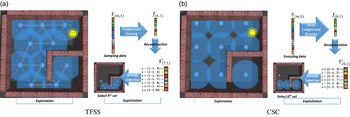
Figure 1 illustrates the concept of TFSS and CSC for search problems, There are two stages for TFSS, exploration and exploitation stages. The exploration stage is to explore the subgoals, while the exploitation stage is to learn the submodular functions and select subgoals. As Fig. 1(a) shows, in the exploration stage, the robot explores 10 subgoals via interacting with environments. In the exploitation stage, the robot selected subgoal#1, 2, and 3. It needs to select the next subgoal with the maximal coverage. Hence, the robot has to predict the coverage of subgoal#4 to #10. The robot batches the sampling data (F) and learns the coverage function in the Fourier domain (f) via compressed sensing. Once the f is learned, the robot can predicts the coverage values (F ′) of the subgoal#4 to #10. Since selecting the subgoal#5 will have the maximal coverage, the robot chooses the subgoal#5 as the next subgoal. The robot keeps selecting the next subgoal until it detects the person. There are two stages for CSC, exploration and exploitation stages. As Fig. 1(b) shows, in the exploration stage, the nine subgoals are assigned manually. In the exploitation stage, the processing is similar to the TFSS. The major difference is that CSC adopts deep compressed sensing (DCS) instead of compressed sensing.
Illustration of the TFSS and CSC approaches. There are two stages, exploration and exploitation stages, in both approaches. Assume the field of view (FOV) and the range of the sensor are
 $360^{\circ}$
and
 $3.5 {\,\rm m}$
, respectively. The environment is a
 $10 \times 10\, {\rm m}^2$
map and the person (simile face) locates in the map. The goal of the algorithms is to detect the person. (a) Exploration: there are 10 explored subgoals. The decimal number represents the number of the visiting sequence. The blue arrows and orange arrows represent the hexagonal directions and the selected explored directions, respectively. In the TFSS approach, the robot explore 10 subgoals via hexagonal packing algorithms. Exploitation: there are 10 explored subgoals. The white decimal numbers represent the index of subgoals. In this case, there are three visited subgoals (subgoal#
 $1\sim3$
). The robot has to decide the next subgoal. Learning
 $\textrm{f}$
via compressed sensing and select subgoals via
 $\textrm{F}$
:
 $\textrm{F}$
represented the m sampling coverage values.
 $\textrm{f}$
is learned after compressed sensing. Once
 $\textrm{f}$
is learned,
 $\textrm{F}^{\prime}$
denotes the predicted coverage values of selecting subgoal#
 $4\sim10$
. In this case, the robot selected subgoal#5, which has the maximal coverage. (b) Exploration: in the TFSS approach, the robot cannot explore the map via interacting with the environment. Hence, the subgoals are assigned manually. There are nine assigned subgoals. Exploration: there are nine explored subgoals. In this case, there are three visited subgoals (subgoal#
 $1\sim3$
). The robot has to decide the next subgoal. Exploitation:
 $\textrm{F}$
represented the m sampling coverage values. f is learned after compressed sensing. Once f is learned,
 $\textrm{F}^{\prime}$
denotes the predicted coverage values of selecting subgoal#
 $4\sim9$
. In this case, the robot selected subgoal#6, which has the maximal coverage.

The contributions of this research are as follows: first, the submodular deep compressed sensing of convolutional sparse coding (SDCS-CSC) is a deep compressed sensing-based appraoch. It is the first approach to apply DCS to people search problems. Second, the advantages and disadvantages of TFSS and SDCS-CSC are discussed. The guideline of how to select the suitable approach is highlighted. Third, experiments conducted with these algorithms demonstrate that the TFSS and SDCS-CSC algorithms can search for the person more efficiently than the benchmark approaches (e.g., spatial Fourier sparse set (SFSS) and SDCS-CNN).
The paper is organized as follows. Section 2 describes the related work. Section 3 introduces the background knowledge. Section 4 describes the proposed search algorithms. Section 5 describes the experiments. Section 6 discusses the advantages and disadvantages of the proposed algorithms. Finally, Section 7 concludes the paper with a summary of the work.
2. Related work
This section first discusses the prior work of spatial search. Since the search problems are reformulated as submodular maximization problems, the prior work of submodularity and how to learn submodular functions are reviewed. Since learning submodular function via compressed sensing techniques is a promising approach, DCS techniques are reviewed. Finally, topological motion planning is reviewed for spatial search in unknown environments.
2.1. Spatial search
How the spatial search problems are solved depends on assumptions about the interactions between the target(s), searcher(s), and environments. Searching in a probabilistic environment (Bayesian search) assumes that the target motion and searcher’s sensing information are probabilistic. The goal is to find the path with the maximal probability to detection [Reference Stone8]. Finding the optimal solutions of probabilistic search is NP-hard [Reference Trummel and Weisinger9].
To take advantages of Bayesian models and the submodularity in coverage problems, the grid map approach was proposed [Reference Tseng and Mettler10]: coverage is computed combining the measurements from sensor positions, real sensing scans, and a known grid map. This problem was shown to be NP-hard [Reference Nemhauser, Wolsey and Fisher1]. Since maximizing coverage is a submodular maximization problem, greedy algorithms are able to achieve solutions over
 $(1-1/e)$
of the optimum. The advantage of this approach is that it provides a near optimal guarantee using real sensor specifications (e.g., range and angle) and works even in cluttered environments.
2.2. Submodularity
Submodularity is that set functions satisfy the diminishing returns property. Greedy algorithms can give solutions with theoretical guarantees for submodular maximization problems under different constraints (e.g., cardinality [Reference Nemhauser, Wolsey and Fisher1], knapsack [Reference Khuller, Moss and Naor3], and routing [Reference Zhang and Vorobeychik4]). The applications include collecting lake information using multiple robots [Reference Hollinger and Sukhatme11], search in indoor environments via graphical models [Reference H, ollinger and Singh12], search in indoor environments via probabilistic models [Reference Tseng and Mettler10], search for humans [Reference Tsai, Lu and Tseng13], and collecting wireless information using UAVs [Reference Hollinger, Choudhuri, Mitra and Sukhatme14].
2.3. Learning submodular functions
The key assumption of aforementioned approaches is that the submodular functions are known. If the submodular functions are unknown, the robot has to learn them online through training samples. However, it is a challenge to learn a submodular function since the number of function outcome from N sets is
 $2^N$
. In ref. [Reference Balcan and Harvey15], the researchers proved that it is impossible to approximate submodular functions accurately within polynomial samples via linear classifiers.
A feasible approach is to learn submodular functions in the Fourier domain [Reference Stobbe and Krause6]. However, the number of Fourier bases is still
 $2^N$
. To solve this issues, wisely selecting the ground set in the spatial domain will have sparsity in the Fourier domain [Reference Tseng and Mettler16]. In other words, the number of Fourier bases could be polynomial if there is a few sensing overlaps. This approach makes learning submodular functions possible [Reference Tseng7]. Nevertheless, when the sensing overlaps are more, the number of Fourier bases is closer to
 $2^N$
. Therefore, spreading the sensors/sets out and adopting DCS are two ways for the basis issue.
2.4. Deep compressed sensing
Due to the successfully applications of deep learning in image classification [Reference Sutskever, Krizhevsky and Hinton17] and learning to play Atari games [Reference Mnih, Kavukcuoglu, Silver, Veness, Graves, Riedmiller, Ostrovski, Petersen, Beattie, Sadik, Antonoglou, King, Kumaran, Wierstra, Legg and Hassabis18], the DCS algorithms have recently been proposed. There are three classes of the DCS approaches.
The first one is the network-based approach. The fully connected and convolution neural networks are applied in DCS. The original signal can be reconstructed with blocks by a deep fully connected neural network [Reference Adler, Boublil and Zibulevsky19]. There are several models of convolutional neural network (CNN) reconstructing the image data from low-dimensional measurements to overcome the disadvantages of traditional compressed sensing methods. For example, designing the sampling matrix and performing optimal signal recovery are challenges. In ref. [Reference Shi, Jiang, Zhang and Zhao20], deep neural networks are proposed to overcome two issues. Reconnet, a non-iterative approach, is proposed to speed up the computation with a novel CNN architecture [Reference Kulkarni, Lohit, Turaga, Kerviche and Ashok21]. Deep Residual Reconstruction Network (
 $DR^2$
-Net) speeds up its computation by adding several residual learning blocks to enhance the preliminary image [Reference Yao, Dai, Zhang, Zhang, Tian and Xu22]. Multi-scale DCS convolutional neural network (MS-DCSNet) is proposed to sampling signal with different scales [Reference Canh and Jeon23]. Since the real-world data could be not exactly sparse in a fixed basis and recovery algorithms are slow to converge, DeepInverse is proposed to overcome these issues via a deep convolutional network [Reference Mousavi and Baraniuk24]. In ref. [Reference Baraniuk and Mousavi25], a stacked denoizing autoencoder with a deep fully connected network is to learn the representation from training data and to reconstruct test data from their CS measurements.
The second one is the frame-based approach. The parameters of iterative soft thresholding algorithm (ISTA) are learned. In ref. [Reference Gregor and LeCun26], the parameters of the encoder and layer-dependent threshold are learnable. In ref. [Reference Ito, Takabe and Wadayama27], the learned parameter is the step size.
The third one combines the above two classes. Iterative soft thresholding algorithm-network (ISTA-Net) [Reference Zhang and Ghanem28] utilizes the advantages of network-based and optimization approaches to design a learnable deep network framework. Instead of handcrafting, the parameters of the autoencoder and networks are learned through the ISTA-Net. In ref. [Reference Tsai and Tseng29], the submodular function is successfully reconstructed by SDCS. The authors proposed a model of deep neural networks to predict the submodular function, which has
 $2^N$
outcome from N sets.
2.5. Topological motion planning
Due to the popularity of topological data analysis, the robotics community has been paying more attention to algebraic topology recently. Although the data vary in the spatial space, the data in the topology has invariant diagrams (so-called persistence homology) [Reference Cohen-Steiner, Edelsbrunner and Harer30]. Utilizing the persistence homology of different trajectories or subgoals/sets could propose different algorithms in motion planning.
Goal-directed path planning in probabilistic maps is one of the robotic problems. Given a probabilistic map, the robot seeks trajectories with persistence homology [Reference Bhattacharya, Ghrist and Kumar31]. How to assign decisions for the cooperative search of a human–robot team is a challenge. The authors proposed algorithms to ensure humans and robots pursue different homotopy classes [Reference Govindarajan, Bhattacharya and Kumar32].
Topology is one of the analysis approaches for coverage problems. To analyze the properties of a sensor network, the researchers proposed Rips complex to detect the holes of the uncovered area [Reference de Silva and Ghrist33]. If the sensor network is for surveyance applications, the evasion path exists when the moving intruder can avoid the covered area. The aforementioned topological analysis for coverage problems are obstacle-free environments. To consider the coverage problems with obstacles, the researchers show that Rips complex-based algorithms can deploy a swarm of mobile robots and attain complete sensor coverage [Reference Ramaithitima, Whitzer, Bhattacharya and Kumar34]. To further consider map exploration in unknown environment, the TFSS was proposed [Reference Lu35]. These successful examples demonstrated that topological tools (e.g., persistence homology) can help analyze robotic problems.
3. Background knowledge
This section first introduces the background of submodular functions. Learning submodular functions via deep learning is described to compress Fourier bases. Topological complexes are introduced for deducing the Fourier bases
3.1. Submodularity of people search problems
The submodularity is defined as follows:
Definition 1:
Submodularity [Reference Nemhauser, Wolsey and Fisher1]. Given a finite set S={1,2,…,n}, a submodular function is a set function
 ${F}\,:\,2^{n} \rightarrow\mathbb{R}$
which satisfies the diminishing return property. For every
 $S_A, S_B\subseteq S$
with
 $S_A\subseteq S_B$
and every
 $s\subseteq S$
,
 $F(S_A\cup s)-F(S_A) \geq F(S_B\cup s)-F(S_B)$
holds.
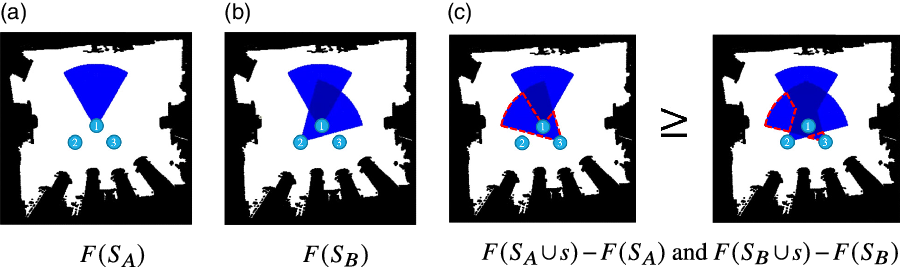
To illustrate the concept of submodularity, an example of environmental coverage is shown in Fig. 2. There are three ground sets
 $(S=\{1,2,3\})$
.
 $S_A=\{1\}$
and
 $S_B=\{1,2\}$
represent the selected two sets, respectively. The set
 $S_B=\{1,2\}$
means that the sensors are selected at location 1 and 2.
 $F(S_A)$
and
 $F(S_B)$
mean the coverage of the sensor(s) at location 1 and
 $\{1,2\}$
(see Fig. 2(a) and (b)), respectively. The submodular gain of
 $S_A$
and
 $S_B$
after adding a set
 $s=\{3\}$
is represented by the red dashing lines (see Fig. 2(c)). It is obvious that the coverage function satisfies the diminishing return property. In other words, the objective function of coverage functions is submodular. Greedy approaches can generate near-optimal solutions even if this is a NP-hard problem [Reference Feige2].
Illustration of the submodularity of coverage functions [Reference Tseng and Mettler16]. The decimal number represents the selected sensor. The blue and white colors represent the covered and uncovered areas, respectively. (a)
 $F(S_A)$
represents the covered area by
 $S_A$
, where
 $S_A=\{1\}$
. (b)
 $F(S_B)$
represents the covered area by
 $S_B$
, where
 $S_B=\{1,2\}$
. (c) The red dash lines represent the submodular gain after adding s, where
 $s=\{3\}$
. Left figure shows the
 $F(S_A\cup s)-F(S_A)$
and right figure shows that
 $F(S_B\cup s)-F(S_B)$
.

Although the submodularity provides theoretical guarantees, coverage functions of unknown environments are not accessible. Hence, the robot has to learn the submodular functions while exploring the environment. This raised another issue – How to learn a submodular function which has
 $2^N$
outcomes?
3.2. Learning submodular functions via compressed sensing
Since submodular functions are set functions, the outcome of submodular functions is
 $2^N$
from N sets, which is a challenging problem in machine learning [Reference Balcan and Harvey15]. In ref. [Reference Stobbe and Krause6], the researchers first proposed Fourier sparse set (FSS) to learn submodular function using compressed sensing techniques [Reference Baraniuk36].
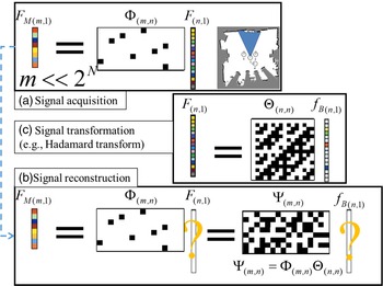
As Fig. 3(a) shows, suppose there are N sets and the submodular function is
 $F_{(n,1)}$
, where
 $n=2^N$
. The robot first acquires a signal from
 $F_{(n,1)}$
via a sensing matrix
 $\Phi_{(m,n)}$
and collects
 $F_{M(m,1)}$
for learning, where
 $m<<n$
. The robot has to predict the submodular function
 $F_{(n,1)}$
(see Fig. 3b). Notice that this is an ill-conditioned linear inverse problem. However, if the signal is sparse in certain domains, the system can recover
 $F_{(n,1)}$
via sparse regression [Reference Tibshirani37]. As Fig. 3(c) shows,
 $F_{(n,1)}$
is the inner product of the transform matrix
 $\Theta_{(n,n)}$
(e.g., Fourier transform) and coefficient
 $f_{B(n,1)}$
. The
 $f_{B(n,1)}$
has only k nonzero values (so-called k-sparse). Since
 $\Theta$
and
 $\Phi$
are known, the reconstruction matrix
 $\Psi$
can be computed. Although directly recovering
 $F_{(n,1)}$
is impossible, the robot can recover
 $f_{B(n,1)}$
if
 $k<m$
, and then reconstruct
 $F_{(n,1)}$
. The learning of submodular functions is given as:
 \begin{align*}\hat{f}_B=\displaystyle\arg\min_{f_B} \frac{1}{2}||F_M-\Psi f_B ||^2+\lambda||f_B||_1\end{align*}
where
 $f_B$
is the submodular function in the Fourier domain,
 $F_M$
is a measurement vector of the submodular function,
 $\Psi$
is a reconstruction matrix (so called dictionary),
 $\Psi=\Phi \Theta$
, and
 $\Phi$
is a sensing matrix and
 $\Theta$
is a inverse Fourier transform matrix.
Illustration of the compressed sensing concept [Reference Tseng and Mettler16]. (a)
 $F_{M(m,1)}$
is collected by the robot after taking measurements from a signal
 $F_{(n,1)}$
. The color cells represent real values and black/white cells represent binary values (0 and 1 in
 $\Phi$
while 1 and -1 in
 $\Theta$
.) (b) The robot has
 $F_{M(m,1)}$
and tries to recover
 $F_{(n,1)}$
. (c) The signal F is sparse in the Fourier domain. In this example, m is 8, n is 16, and k is 4. Given
 $\Phi_{{m,n}}$
and
 $F_{M(m,1)}$
, it is impossible to recover
 $F_{(n,1)}$
(
 $m<n$
). But, given
 $\Psi_{(m,n)}$
and
 $F_{M(m,1)}$
,
 $f_B{(n,1)}$
can be recovered (
 $k<m$
).

However, the size of the Fourier transform matrix is
 $2^N$
by
 $2^N$
, and it is infeasible to compute all of the spectrum. In ref. [Reference Tseng7], the researchers proved that if there is no sensing overlap between sets, the coefficients of the corresponding Fourier basis are zero (see Theorem 1). This approach is called SFSS [Reference Tseng and Mettler16]. The SFSS approach utilizes the sparsity of submodular functions in the Fourier domain to learn submodular functions efficiently.
Theorem 1:
Sparsity of submodular function in the Fourier domain [Reference Tseng7]. If there is no sensing intersection of the sets, the coefficient of the sets’ corresponding Fourier basis is zero. Mathematically, if
 $F(S_{\cap})=0$
,
 $f(S_{\cup})=0$
, where
 $S_{\cap}$
denotes the intersection of sets and
 $S_{\cup}$
denotes the union of sets.
To illustrate the Theorem 1, as Fig. 4 shows, there are four sets (e.g., sensors) in the environments. The number of submodular function values is
 $2^4$
. There are two cases of the ground set in Fig. 4(a) and (b). The order of set is defined as the number of selected sets. The number of
 $n^{th}$
order terms is
 $C^{N}_{n}$
, where N is the total number of sets. Hence, the numbers of
 $0^{th}$
,
 $1^{st}$
,
 $2^{nd}$
,
 $3^{rd}$
, and
 $4^{th}$
order terms are 1, 4, 6, 4, and 1, respectively. In Fig. 4(a), only sets 2 and 3 have sensing overlapping. Hence, only
 $f_{2,3}$
of the
 $2^{nd}$
order terms is nonzero. There is no overlap between the third and fourth order sets, so the Fourier coefficients of
 $3^{rd}$
and
 $4^{th}$
orders are zero. Therefore, the number of nonzero coefficients in case A is
 $1+4+1=6$
. In case B, there is sensing overlapping between all sets. Hence the number of nonzero coefficients in case B is
 $1+4+6+4+1=16$
. This example demonstrates that utilizing the intersection relationship can dramatically reduce the number of Fourier bases from
 $2^N$
to polynomial numbers if there are a few sensing overlaps between sets.
Illustration of the sparsity of submodular functions in the Fourier domain. The black and white areas are obstacles and unoccupied grids, respectively. The black circles and lines represent the robot position and heading, respectively. The blue dash lines are the covered area of the corresponding set/sensor. The colorful and white cells in the bars represent nonzero and zero values, respectively.

The major assumption of SFSS is that if there are a few overlapping sets, the number of Fourier bases can be dramatically reduced. If most sets have sensing overlapping, the number of Fourier basis is still close to
 $2^N$
. Since the SFSS approach adopts Hadamard transform, this transform limits the possibility of Fourier basis selections. To solve this issue, there are two ways. First, spreading the sensors/sets out can dramatically reduce the number of Fourier bases. Hence, proposing a topological algorithm to spread out the sets via is a way. Second, applying nonlinear transform could lead to different sparsity in certain domains. Therefore, designing deep neural networks to compress the functions is another way.
3.3. Learning submodular functions via DCS
Most prior work of DCS is applied to fixed-size signals (e.g., images or videos). For example, to process very high-dimensional images and videos, block-based CS with a fully connected network is proposed as a lightweight method [Reference Adler, Boublil and Zibulevsky19]. Due to the slow processing of sparse coding, in ref. [Reference Gregor and LeCun26], the fast algorithm producing approximate estimation is proposed. ISTA-net is proposed to take the advantages of optimization and network methods [Reference Zhang and Ghanem28]. Trainable iterative soft thresholding algorithm (TISTA) is propose to improve ISTA-net [Reference Ito, Takabe and Wadayama27]. The challenge of DCS techniques for submodular functions is that the networks must avoid processing the original signal since its size is
 $2^N$
. In ref. [Reference Tsai and Tseng29], the researchers first proposed the new network model to learn submodular functions using DCS techniques. Two definitions [Reference Tsai and Tseng29] of learning submodular functions via DCS are as follows:
Definition 3:
Learning submodular functions in the Fourier domain.
Given a finite set S={1,2,…,N}, submodular data (y), and corresponding set data (X), the learning coefficient of the submodular function in the Fouier domain (f) is
 $\hat{f}=min_{f} || \Psi(X,f)-y||_2^2 + \lambda ||f||_1$
, where
 $\Psi$
is a reconstruction function,
 $\lambda > 0$
is the parameter to tune the sparsity of f,
 $|| \cdot ||_2$
is the L2 norm, and
 $||\cdot||_1$
is the L1 norm.
For example, let
 $N=3$
,
 $y=\{0.4, 0.6\}$
, and
 $X=\{0, 0, 1;0, 1, 1\}$
. It means there are three sets. X represents the two selected sets and y represents the corresponding submodular values. When the second and third sets are selected
 $(X=\{0, 1, 1\})$
, its submodular value is 0.6 (
 $y=0.6$
). In fact, this is an ill-conditioned case, since the number of the unknown variable is
 $2^3$
and the number of measurements is 2. If the submodular function in the Fourier domain is sparse, it is possible to learn it in the Fourier domain first and then reconstruct it in the spatial domain. Hence, the goal is to find submodular functions in the Fourier domain (f) first through the given X and y.
Definition 4:
Reconstruction of submodular functions in the spatial domain.
Given a finite set S={1,2,…,N} and corresponding set data (X), the reconstruction of submodular functions in the spatial domain (y) is
 $y=\Psi(X,f)$
.
For example,
 $N=3$
,
 $f=\{0.7, 0.1, 0, 0.2, 0, 0,0, 0\}$
, and
 $X=\{0, 0, 1;0, 1, 0\}$
. The submodular values of correspnding set X can be reconstructed through the given f and
 $\Psi$
function.
The major issues of learning and reconstruction of submodular functions are as follows: first, what is the transform (
 $\Theta$
) that makes the submodule function sparse? Second, what is the transferred submodular function values (f)? Third, how to reconstruct the submodular function (F) through (f)? In order to solve these issues, the researchers proposed SDCS algorithm to learn submodular functions [Reference Tsai and Tseng29]. There are three stages of SDCS: transformation learning, Fourier coefficient learning, and reconstruction.
In the transformation learning stage, the goal is to train the autoencoder model. The network input data is the measured submodular function values in different maps
 $(F_m^{1:M})$
, where m is the size of measurements and M is the number of different environments. The parameters of first and output layers are generated by another little fully connected network (named by weight network W). The input of weight network is the corresponding combination sets of measurements. The Fourier coefficients (f) is the output of the encoder while it is the input of decoder. Mathematically, the transformation is
 $\hat{F}_m^{1:M}=W(X,\theta(f))=\Psi(X,f)$
, where
 $\Psi$
is the reconstruction function, which reconstructs the submodular values given the corresponding f and X. The objective function of transformation learning stage is
 \begin{equation} \begin{aligned} min_{\theta,W} ||{W(X,\theta(f))}-F_m^{1:M}||_2^2\\ \end{aligned}\end{equation}
In the learning Fourier coefficients (f) stage, the algorithm is inspired by ISTA. The trained decoder model is chosen as
 $\Psi$
. There is a random initial f. The back-propagation updates f as
 $\gamma_t$
and the soft thresholding function fix
 $\gamma_t$
as the input f in next iteration. The loss function of this stage is
 \begin{equation} \begin{aligned} min_{f} || \Psi(X,f)-y||_2^2 + \lambda ||f||_1\\ \end{aligned}\end{equation}
In the reconstruction stages, the learned Fourier coefficients (f) are decoded by the decoder
 $\Theta$
. The decoded data
 $\Theta(f)$
and the weighting networks (W) with combinational input (X) generate the reconstruction data (y):
 \begin{equation} \begin{aligned} y=W(X,\Theta(f))=\Psi(X,f)\\ \end{aligned}\end{equation}
To improve the theoretical guarantees, SDCS-CSC is proposed in this research.
3.4. Learning submodular function via multilayer CSC
The assumption of CSC is that the signal has local sparsity in the Fourier domain. The first layer of SDCS-CSC is a fully matrix generated by the input combinations. This structure is similar to the first layer of the SDCS [Reference Tsai and Tseng38]. For the CSC model, the sparsity representation is captured through the
 $\ell_{0,\infty}$
-norm (see Fig. 5). This norm represents the local sparsity of the signal.
The schematic diagram of
 $\ell_{0,\infty}$
-norm.

Definition 5:
 $\ell_{0,\infty}$
-norm [Reference Papyan, Sulam and Elad39]. The
 $\ell_{0,\infty}$
-norm of a global signal
 $\Gamma$
is defined as follows:
 \begin{align*} ||\Gamma||^s_{0,\infty}=\max\limits_{i}||\gamma_i||_0\end{align*}
where
 $\gamma_i$
represents the
 $i^{th}$
stripe vector of
 $\Gamma$
, and
 $||\cdot||_0$
denotes the number of nonzero elements.
There are two parts of SDCS-CSC, sparse coding and dictionary learning. The definition of sparse coding [Reference Papyan, Romano and Elad40] is as follows:
Definition 6:
Submodular deep coding problem.
Given a measurement signal Y, the corresponding set data (X), a set of convolutional dictionaries
 $\{D_i\}^K_{i=1}$
, where
 $D_1$
is generated by X (i.e.,
 $D_1(X)$
), sparse parameters (
 $\lambda$
), and error parameters (
 $\epsilon$
), the definition of the deep coding problem (DCP).
 $DCP^{\epsilon}_{\lambda}$
is defined as:
 \begin{align*} (DCP^{\epsilon}_{\lambda}):\ \text{find}\ \{\Gamma_i\}^K_{i=1}\ \text{s.t.}\end{align*}
 \begin{align*} \qquad ||Y-D_1\Gamma_1|| & \le \epsilon_0, & ||\Gamma_1||^s_{0,\infty} \le \lambda_1 \\ ||\Gamma_1-D_2\Gamma_2|| & \le \epsilon_1, & ||\Gamma_2||^s_{0,\infty} \le \lambda_2 \\ & ... & ... \qquad \\ ||\Gamma_{K-1}-D_K\Gamma_K|| & \le \epsilon_{K-1}, & ||\Gamma_K||^s_{0,\infty} \le \lambda_K \\\end{align*}
The sparse coding finds the representation (
 $\Gamma_i$
) through the given dictionary (
 $D_i$
). The definition of learning dictionary [Reference Sulam, Papyant, Romano and Elad41] is as follows:
Definition 7:
Multilayered dictionary learning. Given a set of measurement signals
 $\{Y^m\}^M_{m=1}$
and the corresponding set data
 $(\{X^m\}^M_{m=1}),$
the objective function of learning dictionary is formulated as:
 \begin{align*}\min\limits_{\{\Gamma_K^m\},\{D_i\}^K_{i=1}} \sum_{m=1}^{M} ||Y^m - D_1(X)D_2...D_K\Gamma_K^m||^2_2\end{align*}
Layered-ISTA is introduced in the Algorithm section for solving
 $DCP^{\epsilon}_{\lambda}$
.
3.5. Hexagonal packing and rips complex
Instead of compressing submodular functions via DCS, another way is to expand the ground set, which has a fewer sensing overlaps. The expanding sets should satisfy two requirements. First, they should cover the environment completely. Second, the number of their sensing overlaps should be as fewer as possible. Assume the sensor range is a disk within r distance in an obstacle-free environment. In ref. [Reference de Silva and Ghrist33], the researchers proved that when the distance between sets equals to
 $\sqrt{3}r$
, the configuration of sets is the optimal solution with the less overlaps and without holes. Generating sets with
 $\sqrt{3}r$
distance is called hexagonal packing [Reference Derenick, Kumar and Jadbabaie42]. The Rips complex represents the geometric properties (e.g., holes). Its definition is as follows:
Definition 8:
Rips complex [Reference Rabadan and Blumberg43].
Given a finite set
 $X \subseteq Y$
in a metric space (e.g.,
 $R^n$
) and
 $r> 0$
. Rips complex R
 $(X,Y;r)$
has
-
1. vertex set X.
-
2. finite simplex
 $\sigma$
when
$diameter(\sigma)\leq 2r$
.


To illustrate the concept of hexagonal packing and Rips complex, assume there is a robot with a sensor covering r distance. The goal is to expand sets via hexagonal packing. As Fig. 6(a) shows, the robot locates at the subgoal#0 and expands subgoals from #1 to #6. Its Rips complex is shown in Fig. 6(b). Since the coverage of each set overlaps with the other two sets, there are six 2-simplex. As Fig. 6(a) shows that there is no hole between seven sets. There is no intersection between three sets, which implies the maximal order is 2. However, the major assumption of aforementioned approach is that the environment is obstacle-free. In ref. [Reference Derenick, Kumar and Jadbabaie42], the researchers proposed a modified hexagonal packing algorithm to expand sets in environments with obstacles. If there is any obstacle along the path, the robot will move back a fixed distance. This approach can be applied to find the ground set of submodular functions in unknown environments.
4. Algorithms
In this section, two algorithms are described. The first algorithm, TFSS, is to expand subgoals and then learn the coverage functions via compressed sensing for selecting the next subgoal. The second algorithm, CSC, is to assign subgoals and then learn the coverage functions via DCS for selecting the next subgoal.
4.1. TFSS algorithms
The overall of TFSS algorithms is illustrated as Fig. 1(a) and Algorithm 1. In the exploration stage, the robot expands the subgoals via the hexagonal packing algorithm (Algorithm 2 and Fig. 6(a)). In the exploitation stage, the robot needs to learn the coverage function and select the next subgoal for finding the person. The robot acquires and saves the sensing data in the database. It samples the coverage data (
 $F_M$
) from the database and learn the coverage function (f) in the Fourier domain. To select the next subgoal with the maximal coverage, the robot needs to predict the coverage values of subgoal candidates. The robot reconstructs the coverage values (F
′) of subgoal candidates and selects the subgoal with the maximal coverage until finding the person or the cost is over the budget.
TFSS algorithm.

Illustration of Hexagonal packing and Rips complex. (a) The robot locates at set#0 and is expanding six sets via the hexagonal packing. The black nodes and blue areas represent sets and their coverage, respectively. The dark blue areas are the overlapping areas. The orange arrows and the numbers represent the hexagonal packing direction and the ordering of selected sets, respectively. (b)The blue lines and yellow triangle represent 1-simplex and 2-simplex, respectively.

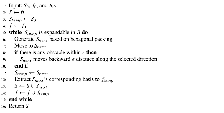
The details of TFSS algorithms are as follows: Algorithm 1 shows the TFSS algorithm. Lines4–6 show the exploration stage. The robot expands subgoals until the environment is explored (see the exploration in Fig. 1(a) and Fig. 6(a)). Lines 8–18 show the exploitation stage (see the exploitation in Fig. 1(a)). Lines 8 shows the robot keeps moving to subgoals until the number of subgoal
 $(|S_G|)$
is over the G. Lines 11–13 show the robot saves the explored subgoals to the database. Line 14 shows that the robot randomly generates A and
 $F_M$
data during its flight, where A is the measurement sets and
 $F_M$
is the corresponding coverage data of A. These data are based on the robot’s point cloud data from the Red Green Blue Depth (RGBD) sensor. Hence, A and
 $F_M$
data will be used to learn the coverage function in this environment. Line 16 shows once the robot arrives at the subgoals, it will call
 $SFSS\_subgoal$
function to compute the next subgoal. Finally, if the robot detects the person or the cost is over the budget, the robot terminates its search.
Algorithm 2 shows the subgoal expansion algorithm. Lines 2–4 show the initialization of S and f. Lines 6–7 show the hexagonal packing (see Fig. 6). The robot will expand explored nodes through six directions. Lines 8–10 show the hexagonal packing when there is any obstacle. The robot will move back a fixed distance
 $(\epsilon)$
from the original explored subgoal. Lines 11–14 show the new S and f are saved. After running this algorithm, the robot explored subgoals in the boundary
 $(B_O)$
.
ubgoal expansion algorithm.

The initialization of f is as follows: since the map is unknown in exploration problems, it is difficult to compute the values of f. In ref. [Reference Tseng7], the author proved the sparsity of submodular function in the Fourier domain and further show that the f in an empty map can be used for the initial values of f in any maps.
In other words, the robot can predict initial values of f without any map information. Therefore, the initial f is set as the values of
 $f_0$
in an empty map.
Algorithm 3 shows the
 $SFSS\_subgoal$
algorithm. Lines 3–7 show the basis matrix (
 $\Psi$
) is computed according to A and B, where A is the sets of sampling data and B is the sets of Fourier basis. Line 9 shows that the submodular function in the Fourier domain
 $\hat{f}$
is computed via sparse regression. Lines 12–13 show that the submodular function in the spatial domain F(S) is reconstructed. Lines 14–16 show if the cost is satisfied, the set with maximal coverage rate will be selected. Line 19 shows that the algorithm returns the next subgoal
 $S_{G,k+1}$
and the updated
 $\hat{f}_B$
.
SFSS subgoal algorithm.

4.2. Submodular deep compressed sensing of convolutional sparse coding algorithms
The overall of the proposed SDCS-CSC algorithms is illustrated as Fig. 1(b). In the exploration stage, the subgoals are assigned manually. In the exploitation stage, the robot needs to learn the coverage function and select the next subgoal for finding the person. The robot acquires and saves the sensing data in the database. It samples the coverage data (
 $F_M$
) from the database and learn the submodular function (f) in the Fourier domain via neural networks. To select the next subgoal with the maximal coverage, the robot needs to predict the coverage values of subgoal candidates via the forward propagation. The robot reconstructs the coverage values (F
′) of subgoal candidates and selects the subgoal with the maximal coverage until finding the person or the cost is over the budget.
This algorithm combines the model of ref. [Reference Tsai and Tseng29] and the method framework of ref. [Reference Papyan, Romano and Elad40]. There are two algorithms for learning sparse coefficients and dictionary: layered-ISTA and convolutional dictionary learning. In the layered-ISTA (Algorithm 4), the goal is to compute the sets of sparse representations,
 $\{\Gamma_i\}_{i=1}^K$
, through training data. The training data are the coverage data from a measurement set (y). Line 3 is to set the measurements (y) as
 $\hat{\Gamma}_0$
. Line 4–14 show that the sparse representations are computed layer by layer. Line 4–8 are similar to Line 10–14. Since
 $D_1$
is generated by X, the notation is different. Line 10 is to set the sparse representation as 0. Line 11–13 run the gradient descent with a given dictionary and soft-thresholding for epoch times. The sparse representation of this layer is adopted to find the sparse representation of the next layer.
The layered iterative soft thresholding.

The goal of Algorithm 5 is to find suitable dictionaries, which is similar to
 $\Psi$
matrix in TFSS. The layered-ISTA computes the set sparse representations of each layer with given dictionaries. Line 5 is computed the sparse representation for each layer by Algorithm 4. Line 6–13 show the dictionaries are updated from the last to the first layer.
Convolutional dictionary learning.

Algorithm 6 shows the CSC_subgoal algorithm for one iteration. In this algorithm, the dictionary is trained by training data and the sparse coefficient is learned. In Line 4, the sparse coefficients is learned by the measurement got in this iteration, while the initial value is the learned coefficients in last iteration. Line 6 shows that the coverage function is reconstructed by X (depends on S), learned dictionary (
 $\{D_i\}^L_{i=1}$
), and sparse coefficients. Line 7–8 show that the argument maximum is found to do greedy algorithm. After this algorithm, the robot can get the selected subgoal. If the Line 16 in Algorithm 1 is replaced by
 $CSC\_subgoal$
, it is the search algortihm via SDCS-CSC.
CSC subgoal algorithm.

5. Experiments
To evaluate the performance of proposed algorithms, there are three major experiments in this research. EX1, the reconstruction experiment, evaluates the learning performance of the proposed algorithms SDCS-CSC and the prior works (e.g., SFSS [Reference Tseng and Mettler16] and SDCS-CNN [Reference Tsai and Tseng29]). EX2 and EX3 are evaluated by the expected time to detection (ETTD) [Reference Chung and Burdick44] and success rate. EX2, search with dense subgoals, evaluates the search performance when subgoals are close. The performance of SDCS-CSC, and SFSS is compared in a Gazebo simulator and a real-world environment. EX3, search with sparse subgoals, evaluates the search performance when subgoals are explored by TFSS. The performances of SDCS-CSC and TFSS are compared in a Gazebo simulator and a real-world environment. In other words, EX2 and EX3 are compared with the SDCS-CSC and SFSS performance when the subgoals’ distributions are different.
5.1. Experimental setup
In EX1, the maps and subgoals configurations are as follows: The experimental environments are
 $300\times300$
grid maps (see Fig. 7). The Map-1 is adopted for training
 $\Theta$
. Map-0 is adopted for training f and testing reconstruction results. The subgoal configuration is shown in Fig. 7(c). The range and field of view for each subgoal are 75 and
 $60^{\circ}$
, respectively. There are nine subgoals with six directions for each subgoal (i.e., there are
 $54(9\times6)$
subgoals). The distance of two adjacent subgoals is 20 units.
The experimental environments. The black and white grids represent the occupied and unoccupied grids, respectively. (a) A grid map built in a Lab environment. (b) A grid map without any obstacles. (c) The subgoal configuration in the experiment. The red points represent the subgoal locations. The black and white grids represent the occupied and unoccupied grids, respectively. The blue areas and red lines represent the areas covered and field of view, respectively. The sensor-covered radius is 75 and the distance between subgoals is 20.

The training data are collected by 3000 set combinations, which are randomly selected. The distributions of each subgoal’s frequency and the order of the combinations are shown in Fig. 8. There are 500 different training maps (see Fig. 9) which are randomly generated obstacles in Map-1. The random selected 100 different training maps in each batch. The input dimension of the transformation learning stage is
 $100\times3000$
in every batch.
The distribution of 3000 test data. The subgoal is chosen uniformly, and the order is normal distribution.

The training data for the transformation learning stage. The black areas represent different obstacles in each map.

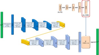
Since the network structures of the Fourier coefficient learning and reconstructions stages are similar to that of the transformation learning stage, the network structures of the transformation learning stage are explained as follows (see Fig. 10): this stage includes an autoencoder, weighting networks (W), and combinational networks. The autoencoder is implemented by the CNN.
Convolutional neural network (CNN) [Reference Tsai and Tseng29]. The frameworks of the transformation learning. This stage includes an autoencoder, weighting networks (W), and combinational networks.

The structure of the SDCS-CNN autoencoder [Reference Tsai and Tseng29] is as follows (see Fig. 10): the first layer and the output layer are fully connected. There are four convolution layers in the encoder and four deconvolution layers in the decoder. In each hidden layer, the filter size of a channel is 1
 $\times$
6 and the stride is 1
 $\times$
4. The activation functions in the output layer of encoder and decoder are soft threshold functions with
 $\lambda=0.01$
and sigmoid function, respectively. The numbers of filters in each layer in the encoder are 16, 32, 64, and 64.
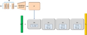
The structure of the SDCS-CSC is as follows (see Fig. 11):
 $D_0$
is fully connected matrix. There are three convolution layers (
 $D_1, D_2, D_3)$
. In each convolution layer, the stride is 1
 $\times$
5. In the first and third layers, the filter size of a channel is 1
 $\times$
7, while the filter size of a channel is 1
 $\times$
5 in the second layer. The numbers of filters in each layer in the encoder are 1, 8, 16, and 32. The prediction errors are computed by 5000 different set combinations (Fig. 12) in Map-0.
The framework of the SDCS-CSC model.

The distribution of 5000 test data. The subgoals are chosen uniformly, and the order of subgoals is normal distribution.

5.2. EX1: Reconstruction experiments
The performance metrics are the mean error of estimated coverage, the results of the greedy algorithm, and the number of Fourier support (nonzero coefficients). For each approach, the number of all subgoals
 $(|S|)$
is 54. Selecting the optimal solutions of three approaches is infeasible, since it needs to compute
 $|54|^G$
solutions where G is the number of selected subgoals. The coverage of selected subgoals of four approaches is compared with G = 15. Hence, the greedy algorithms are adopted for the three approaches to finding near-optimal solutions [Reference Feige2].
In this experiment, the distance between two adjacent subgoals is 20, and the number of Fourier basis (b) of SFSS is 9852; it is decided by the algorithms in ref. [Reference Tseng and Mettler16]. The number of bases (
 $|f|$
) of SDCS-CNN is 384. The different thresholds (
 $\lambda$
) are tested to get the reconstruction in the Fourier coefficient learning stage. The thresholds are set as follows: SDCS-CNN: [1e-5, 0.001, 0.005, 0.01, 0.05, 0.1, 0.15, 0.3, 0.6]; SDCS-CSC: [1e-10,1e-9,1e-8,1e-7,1e-4]; and SFSS: [1e-5, 0.001, 0.0015, 0.002, 0.0035, 0.005, 0.01].
5.2.1. Reconstruction results versus sparsity
As Fig. 13 shows, when the number of nonzero elements in f is lower than 400, the mean error of SDCS-CSC is lower than that of SDCS-CNN and SFSS. In addition, the mean error of SDCS-CSC is lower than that of SFSS even the nonzero elements of SFSS is more than 1000. These experiments demonstrate that SDCS-CSC approach is able to reconstruct submodular functions using fewer Fourier bases than the SFSS approach and the SDCS-CNN does.
When the distances of two adjacent subgoals are 20, the figure shows the k-sparse in transferred coefficient versus mean error between reconstructed result and ground truth in Map-0 and two different numbers of measurements. The reconstruction resulted in 500 and 1000 measurements in Map-0 (Fig. 7(a)).

5.2.2. Greedy results versus sparsity
The reconstruction results with lower errors does not mean that the coverage of selected subgoals (so-called greedy results) is higher. The k is defined as the number of Fourier supports. The test data are 1000 measurements in Map-0 (see Fig. 14). The reconstruction error and greedy results of three approaches are further compared with different
 $\lambda$
parameters.
Comparisons of results of three approaches.

As Fig. 14(a) shows, when the reconstruction error of three approaches is around 0.009, their greedy results are similar. The number of nonzero elements of SDCS-CSC is just 3, which is smaller than that of SDCS-CNN and SFSS. The coverage area in the Map-0 of each approach is shown in Fig. 15. The greedy results of SDCS-CSC approach are similar to those of SDCS-CNN and SFSS, while the k of SDCS-CSC is lower than that of SDCS-CSC and SFSS (3 vs. 45 vs. 408). The error of SDCS-CSC is around 0.009, but the greedy result is similar to ground truth (see Fig. 16(d)) and other approaches.
Coverage area is shown in Map-0 with Fig. 14(a). The black and white grids represent the occupied and unoccupied grids, respectively. The blue grids represent the coverage area of the sensor. The grid being dark blue means that this grid is covered by at least two sensors. The green circle and red cross represent the subgoal being selected or not.

Coverage area is shown in Map-0 with Fig. 14(b).

As Fig. 14(b) shows, the performances of the three approaches with the smallest
 $\lambda$
values in Section 5.2.1 is compared. The reconstruction error of SDCS-CSC is less than that of SFSS and SDCS-CNN, while the greedy results are similar. This experiment demonstrates that SFSS and SDCS-CNN can be replaced by SDCS-CSC (see Fig. 16).
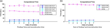
5.2.3. Computational time
The execution time for the three approaches is calculated. All approaches are implemented via Python on a workstation. The execution time includes learning the Fourier coefficients and reconstruction. The time of training transform and collecting the training data in SDCS and the time of finding the basis in SFSS are not considered. The time finding 30 subgoals is calculated via the greedy algorithm to represent the reconstruction time. There are seven different thresholds (1e-10, 1e-9, 1e-8, 1e-7, 1e-6, 1e-5, and 1e-4) for SDCS-CSC, while those of other two methods are (1e-5, 0.0001, 0.0005, 0.001, 0.005, 0.01, and 0.05). For each approach with each threshold, the execution time for 10 times, mean and the variance are calculated. Figure 17 shows that SFSS needs more time to find the coefficient and do reconstruction. Since the
 $\Psi$
matrix is computed by sampling and basis combination where the number of SFSS basis is 9852 in this experiment, SDCS is faster than SFSS. This experiment shows that SDCS approaches are more efficient than SFSS when most of the sets’ sensing areas are overlapped. Among them, the SDCS-CSC model is the most efficient one in the computational time.
Computational time of three approaches

5.3. EX2: Search with dense subgoals
The SFSS approach in ref. [Reference Tseng and Mettler16] and SDCS-CNN approach in ref. [Reference Tsai and Tseng38] are adopted as the benchmark to compare with the proposed algorithm (SDCS-CSC) in the Gazebo simulator and real-world environment. To compare the ETTD for three approaches, the target is a person who appeared at five different locations (see Fig. 18(a)). For each search, the number of total subgoals (
 $|S|$
) is 114 and the number of selected subgoals (G) is 20. Greedy algorithms are adopted for the two approaches to finding near-optimal solutions. For each approach, the robot searches for the person 10 times in one epoch. For the first five times, the robot searches with exploration via
 $\epsilon$
-greedy where
 $\epsilon$
is set as 0.4 (i.e., the subgoal is uniform randomly selected with the probability 0.4). The training f data are generated by all visited subgoal in the epoch. Then the ETTD is compared in the last five times which solution is selected by the greedy algorithm, since the goal of the first five times is to learn the f. There are three epochs in the Gazebo simulator and two epochs in the real-world environment.
5.3.1. Experimental setup
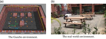
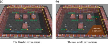
The experimental environments of the Gazebo simulator and real-world maps are shown in Fig. 18. The Gazebo environment is generated with reference to the real environment. The dimension of the environment is
 $13{\, \rm m}\times 10{\, \rm m}$
. The experimental parameters are as follows (see Table I). The number of subgoal ground set (
 $|S|$
) and selected subgoal(G) are 114
 $(19\times6)$
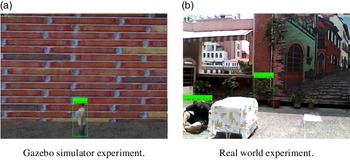
and 20, respectively. The number of SFSS Fourier basis is 7840. In this experiment, the training data of SDCS-CNN autoencoder model and SDCS-CSC model are collected by 6000 set combinations, which are randomly selected. The 1000 training 3D maps are randomly generated obstacles in the empty map which dimension is same as the experimental environment. The structures of CNN autoencoder and CSC model are same as Section 5.2. In the Gazebo simulator, the robot platform is a 3DR IRIS drone model with an R200 RGBD sensor. In the real-world environment, it is an Intel Ready to Fly Drone. The RGBD sensor is to access the real-time RGB image for detecting the person via an Intel neural stick which detects persons through the MobileNetSSD model (see Fig. 19).
Experimental parameters.

The experiment environment is 13
 $\times$
10 (
 ${\rm m}^2$
). (a) The red stars and blue smile faces represent the subgoal and person locations, respectively. (b) The subgoals’ and persons’ locations are same as Gazebo.

The search processing is as follows: the drone takes off and moves to the
 $1^{st}$
subgoal. Once the drone arrives at the
 $1^{st}$
subgoal, it will hover for 5 s. The Bayes filter updates the probabilty of the person (T) in this image
 $P(T=1)$
at
 $20\,{\rm Hz}$
based on the detection outcome. If the person is not found (
 $P(T=1) <P_{th}$
), the drone will move to the next subgoal. Once the person is found (
 $P(T=1) \geq P_{th}$
) or cannot find the person after arriving at the 20th subgoal, the search is terminated and the drone will land on the ground. The search time (time to detection) is defined as the time between taking off and landing. After a search processing, the f is trained by 500 set combinations which is random generated by all visited subgoal in the epoch.
5.3.2. Expected time to detection and successful rate
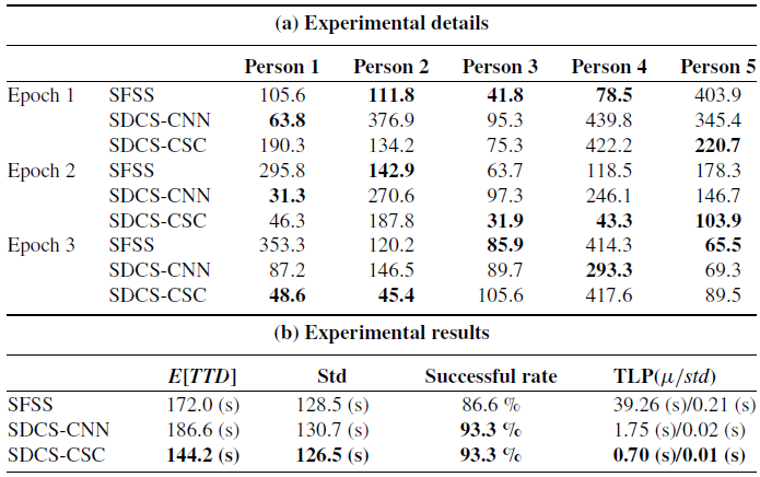
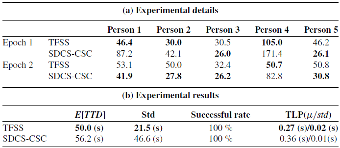
The experimental results in the Gazebo simulator are summarized in Table IIb. The ETTD of the SDCS-CSC is 16% faster than that of the SFSS algorithm, and the time of learning f and prediction (TLP) of the SDCS-CSC is 98% faster than that of the benchmark algorithm. Although the ETTD of the SDCS-CNN is 7% more than that of the benchmark algorithm, the time of learning f and prediction (TLP) of the SDCS-CNN is 96% faster than that of the benchmark algorithm. The successful rate of the proposed algorithms is 6% more than that of the benchmark algorithm. In Fig. 20(a), the coverage of subgoals selected by SDCS-CSC and SDCS-CNN are higher than that of SFSS when the measurements are generated by visited subgoals.
Gazebo environment with dense subgoals.

The detected images. The green rectangles and decimal numbers represent the detected area and corresponding probability, respectively.

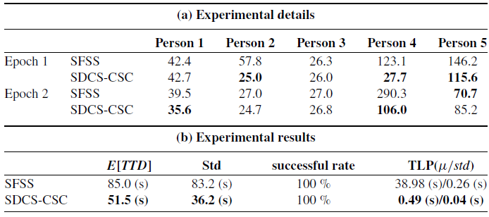
The experimental results in the real-world environment are summarized in Table IIIb. The ETTD of the SDCS-CSC is 40% faster than that of the SFSS algorithm, and the time of learning f and prediction (TLP) of the SDCS-CSC is 98% faster than that of the benchmark algorithm. In Fig. 20(b), the coverage of subgoals selected by SDCS-CSC is higher than that of SFSS when the measurements are generated by visited subgoals.
Real-world enviornment with dense subgoals.

The greedy results with dense subgoals.

These experiments demonstrate the following facts: first, the time of learning f and predicting coverage of SDCS-CSC is faster than that of the SFSS algorithm and the greedy results are better than the SFSS, while the search performances of three algorithms are similar. Second, the recovery performance of the SDCS-CSC is higher than that of the SFSS in the simulator and real-world environment under dense subgoals cases.
5.4. EX3: Search with sparse subgoals
The TFSS and SDCS-CSC approaches are compared in the Gazebo simulator and real-world environment. In this experiment, the numbers of total subgoals (
 $|S|$
) in Gazebo and real world are 42 and 36, respectively. The number of selected subgoals (G) is 20. The subgoals and persons’ locations are shown in Fig. 18 For each approach, the robot searches for the person 10 times in one epoch. For the first five times, the robot searches with exploration via
 $\epsilon$
-greedy where
 $\epsilon$
is set as 0.4. The training f data are generated by all visited subgoal in the epoch. Then, the ETTD is compared in the last five times which solution is selected by the greedy algorithm, since the goal of the first five times is to learn the f. The search processing is same as Section 5.3.
5.4.1. Experimental setup
The experimental environments of the Gazebo simulator and real-world maps are shown in Fig. 21. The dimension of the environment is
 $13{\, \rm m}\times10{\, \rm m}$
. The experimental parameters are as follows: the subgoals are explored by hexagonal packing (Algorithm 2). Therefore, the configurations of subgoals in Gazebo and real world are different. The numbers of subgoal ground set (
 $|S|$
) of Gazebo and real world are 42
 $(7\times6)$
and 36
 $(6\times6)$
, respectively. The number of selected subgoal(G) is 20. The SFSS Fourier basis size is 64. In this experiment, the training data of SDCS-CSC model is collected by 3000 set combinations, which are randomly selected. The 3D maps, robot platform, and all sensors are same as Section 5.3.
5.4.2. Expected time to detection and successful rate
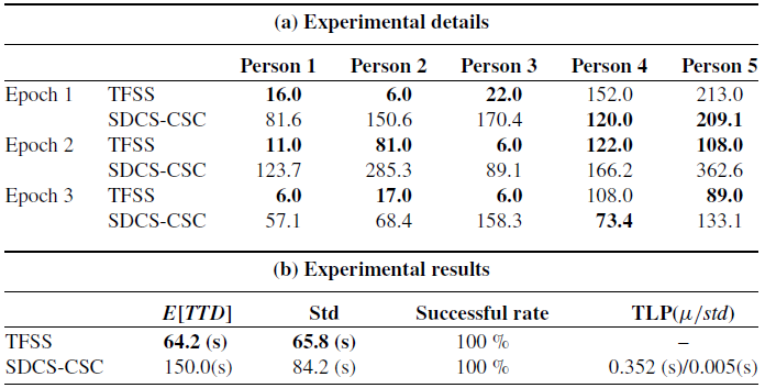
The experimental results in the Gazebo simulator are summarized in Table IVb. The ETTD of the TFSS is 57% faster than that of the SDCS-CSC algorithm. The successful rate of the SDCS-CSC and the SFSS algorithm are 100%. Since the number of Fourier basis is just 64, the time of learning f and predicting coverage of TFSS is as fast as SDCS-CSC while the performance of TFSS is better.
Gazebo enviornment with sparse subgoals.

The experiment environment is 13
 $\times$
10 (
 ${\rm m}^2$
). (a) The red stars and blue smile faces represent the subgoal and person locations, respectively. (b) It is is same as Fig. 18(b). The real-world subgoals’ configuration is shown in the Gazebo environment.

The experimental results in the real-world environment are summarized in Table Vb. The E[TTD] of the TFSS is 11% faster than that of the SDCS-CSC algorithm, and the time of learning f and prediction (TLP) of the SDCS-CSC is similar as that of the TFSS algorithm. In Fig. 22, the coverage of subgoals selected by SDCS-CSC and TFSS are similar when the measurements are generated by visitedsubgoals.
Real-world environment with sparse subgoals.

The greedy results of SDCS-CSC and TFSS with sparse subgoals.

These experiments demonstrate that the recovery performance of the SDCS-CSC is similar to that of the TFSS in the real-world environment under sparse subgoals cases. Due to the coverage performance (see Fig. 22), the search performance of TFSS is better than that of SDCS-CSC.
5.5. Comparison with algorithms
The SFSS was proposed for learning submodular functions and applied to search problems [Reference Tseng and Mettler16]. However, when there are more overlapping between sensing areas, the number of Fourier support increases exponentially [Reference Tseng7]. To overcome this issue, there are two ways, spreading out the subgoals in the spatial domain and compressing the submodular functions in the Fourier domain. The first approach is TFSS via topology, while the second one is CSC via deep learning.
The accuracy of submodular function is the major factor affecting the search behavior. Hence, the recovery performance of SFSS, TFSS, and CSC is discussed under three cases, full Fourier support, dense subgoals, and sparse subgoals. In the full Fourier support, each approach has all Fourier support. The recovery performance of SFSS and TFSS is exact recovery. However, even if CSC has full Fourier support, it cannot exactly recover submodular functions due to the nonlinear and lossy compression. Therefore, in this case, their recovery error is
 $e_{CSC}>e_{TFSS}=e_{SFSS}\sim0$
.
In the dense subgoals case, the SFSS needs to discard parts of Fourier support for alleviating computational issues, so its accuracy degrades. The CSC can compressed the submodular function even if the subgoals have a lot of overlapping areas. The TFSS automatically decides the distance between subgoals. Hence, there is no dense subgoal case for the TFSS. Hence, in this case, their recovery error is
 $e_{SFSS}>e_{CSC}$
.
In the sparse subgoals case, the SFSS has all Fourier support. It can exactly recover submodular functions. The CSC is a nonlinear and lossy compression approach, so it cannot exactly recover them. The TFSS can have all Fourier support. Hence, it can exactly recover them also. In this case, their recovery error is
 $e_{CSC}>e_{TFSS}=e_{SFSS}\sim0$
. To further analyze the search behavior of the CSC and TFSS, locations of their subgoals are important. Since TFSS is based on the hexagonal expansion, generating the minimal Fourier support, the number of TFSS Fourier support is less than or equal to that of SFSS Fourier support. This leads to fast computation of TFSS. Since the number of TFSS subgoals is less than or equal to that of SFSS subgoals, the UAV with TFSS could fly to far subgoals and then detect the target. Hence, the search behavior of TFSS could lead to slower search speed.
6. Discussion
The TFSS and CSC are based on compressed sensing techniques. This section discusses their advantages, disadvantages, and potential applciations.
6.1. Selecting CSC or topological Fourier sparse
Since the TFSS and CSC are based on topology and deep learning, respectively, they have different advantages and disadvantages. To help users for selecting TFSS or CSC, a guideline is described in this subsection.
6.1.1. Advantages and disadvantages of topological Fourier sparse for people search
The advantages of TFSS are as follows: first, it can generate dynamic subgoals via interacting with environments. Hence, it can be applied to search problems in unknown environments. Second, since it is based on linear transform (e.g., Hadamard transform), the Fourier bases can be computed via the sensing overlaps of subgoals offline. Third, it can exactly recover coverage functions if all Fourier supports (
 $|f|$
) are kept for compressed sensing algorithms [Reference Tseng7].
The disadvantages of TFSS are as follows: first, the number of Fourier bases increases when the sensing overlaps of subgoals increases. Hence, the number of Fourier bases could be close to
 $2^N$
, which is infeasible for online computations. Second, if the number of Fourier bases is too large to run algorithms online, the users can discard parts of Fourier bases. However, the accuracy of submodular functions will be decreased if
 $|f|$
is smaller.
6.1.2. Advantages and disadvantages of CSC for people search
The advantages of CSC are as follows: first, it can compress submodular functions with a fixed number of Fourier bases (
 $|f|$
). Second, since its
 $|f|$
is small (e.g.,
 $200\sim400$
), its reconstruction computation (forward propagation) is fast.
The disadvantages of CSC are as follows: first, the ground set (S) needs to be fixed. Once the set in S is changed, the parameters of CSC need to be retrained. Hence, it is only applied to the given maps. Second, since the parameters of CSC are more than that of TFSS, it needs more data and time for pre-train. Third, it is one kind of distortion compression algorithms, which means it cannot exactly reconstruct the submodular functions.
6.1.3. The guideline of selecting CSC or TFSS
The guideline of selecting TFSS or CSC for people search problems is as follows (see Fig. 23): first, if the map is not given, selecting TFSS to generate subgoals/sets of coverage functions. If the map is given, the next step is to assign the subgoals and generate Fourier bases. Second, if the number of Fourier bases (
 $|f|$
)is over than
 $N_B$
, the computation of compressed sensing cannot run online. For example, for a
 $2.6\,{\rm GHz}$
CPU, if
 $|f|$
is over 3000, the computational time could over 1 s, which is impractical for real-time search processes. Therefore, if
 $|f| > N_B$
, the users need to reassign the subgoals, which are spread out so that the coverage functions are sparse in the Fourier domain. After reassigning subgoals and regenerating Fourier bases, if
 $|f| > N_B$
, selecting CSC to compress the submodular functions with a fixed
 $|f|$
. If
 $|f| \leq N_B$
, the users should select TFSS to get more accurate approximation of submodular functions.
The flowchart of selecting TSSS or CSC.

6.2. Links between problems, experiments, and conclusion
The outcome of submodular functions for N sets is
 $2^N$
in the spatial domain. SFSS transfers functions to the frequency domain, which compressed the data to a computable level. However, the number of Fourier coefficients increases when the subgoal/set distribution is closed. To solve this issue, there are two ways. The first way is to compress submodular functions in the Fourier domain via the nonlinear transform methods. The second way is to spread subgoals/sets out in the spatial domain via the topological methods.
SDCS-CSC is to compress submodular functions by deep neural networks. The number of Fourier coefficients compressed by SDCS-CSC is fewer than that by SFSS. The fewer number of Fourier coefficients makes the reconstruction of SDCS-CSC faster than that of SFSS. Hence, SDCS-CSC can outperform SFSS when the subgoal distribution is desne (EX2).
TFSS is to spread subgoals out via Rip complexes and the hexagonal packing algorithm. The hexagonal structure of subgoals lets sensors cover the environment completely, and the number of sensing overlaps is as few as possible if there is no obstacle. The subgoal distribution generated by TFSS has fewer Fourier bases than that generated by manual. The fewer number of Fourier coefficients makes the reconstruction of TFSS faster than that of SFSS. Hence, TFSS can outperform SFSS when the subgoal distribution is sparse (EX3).
6.3. Potential applications
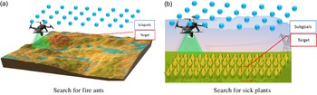
Proposed algorithms can be applied in scenarios, while objective functions of the applications satisfy submodularity. For example, the invasive fire ants have expanded their territories in Asia and affect the original ecosystem. They are also harmful for humans. UAVs are suitable platforms for detecting them. As Fig. 24(a) shows, there is a 3D map and predefined subgoals. Given a fixed budget (e.g., time), the UAV has to find the fire ants as soon as possible. TFSS and CSC can be applied to search for the fire ants.
Illustration of two applications. The red areas and blue points represent the target and the subgoals, respectively.

To give another example, normalized difference vegetation index (NDVI) is adopted to measure the healthy status of plants. However, to build a complete NDVI image by humans is difficult. Hence, letting a UAV collect the NDVI information is a promising way. As Fig. 24(a) shows, there is a farm and predefined subgoals. Given a fixed budget (e.g., time), the UAV has to find the sick plant as soon as possible via NDVI. TFSS and CSC can be applied to search for the plant.
6.4. Tuning the parameters
The framework of deep neural network is based on the method in ref. [Reference Zhang and Ghanem28]. Each parameter in the network are tuned, while other parameters are fixed. First, the learning rate (
 $\beta$
) is tuned by the bisection method. Second, the activation function is chosen after testing all major functions (e.g., tanh, sigmoid, etc.). Third, the distance (d) between adjacent subgoals is decided depending on the sensor range and the number of overlap.
6.5. Applying algorithms to a new environment
Each environment has its own sparse representation sets. Hence, the sparse representations (
 $\Gamma$
) need to be retrained with trained nerual network (Algorithm 6) once the new environment was involved. There are three steps of SDCS-CSC. The first step is to train the dictionary (D). The dictionary is trained by many different environments’ coverage functions. The second step is to learn the sparse representations (
 $\Gamma$
). Sparse representations of the new environment are learned by trained dictionaries and collected data. Sparse representations are learned when the agent explores the new environment. The third step is to reconstruct the coverage function by learned sparse representations. After training, the coverage function of the new environment can be predicted by learned sparse representations.
7. Conclusions
This research proposed SDCS-CSC and applies TFSS to people search problems. These algorithms include two stages, exploration and exploration. The exploration is to find the subgoals in the map, while the exploitation is to learn the coverage functions for selecting the next subgoals until finding the person. Since the TFSS is based on topological and compressed sensing techniques, it can dynamically generate subgoals via interacting the environments. On the contrary, the SDCS-CSC is based on DCS techniques. Therefore, it can compress the submodular functions to a fixed number of the spectrum. Experiments show that TFSS and SDCS-CSC can search for the person more efficiently than the benchmark approaches (e.g., SFSS and SDCS-CNN).
The future work is as follows: first, state-of-the-art DCS techniques cannot be applied to dynamic subgoals of submodular functions (e.g., TFSS). If the spatial relationships of subgoals in the deep neural networks are explored, the SDCS-CSC approach could be applied to search problems in unknown environments. Second, learning submodular functions via deep neural networks is still a challenge [Reference Tsai and Tseng38] and needs a lot of data and time. If the transfer learning of deep learning is explored for learning submodular functions, it could reduce the preprocess (e.g., basis generator) and be applied to various applications. Finally, since humans are able to explore environments efficiently, exploring how humans solve exploration problems is another way to investigate search problems. A promising approach is to let human subjects remotely control the robot and search for the person [Reference Tseng and Mettler45]. These data could be adopted to compare human and robot performance [Reference Tseng and Mettler46]. The coordination patterns between gaze and control in human spatial search can be further analyzed [Reference Tseng and Mettler47]. To analyze 3D search behavior, a UAV is remotely controlled by the human subject for collecting data [Reference Lu, Wu, Tsai, Jiang and Tseng48]. The collected human data can be also adopted for deep inverse reinforcement learning [Reference Wulfmeier, Ondruska and Posner49]. If the search behavior is learned, the deep neural networks can be applied to autonomous search.
Conflicts of Interest
None.
Financial Support
This research was completed thanks to the financial support from Taiwan MOST Grant 108-2221-E-008-074-MY3.
Ethical Considerations
The ethical review was approved by Research Ethics Committee of National Taiwan University. NTU-REC No.: 201811ES028.
Authors’ Contributions
Bing-Xian Lu and Yu-Chung Tsai contributed equally.