Implications
Two algorithms for genomic selection of moderately sized populations are described, and applied to the analysis of milk, fat and protein production; somatic cell score (SCS); female fertility; persistency; and herd-life of Israeli Holsteins. Method II genomic evaluations were less biased and more accurate than parent averages for fat, protein, female fertility, persistency and herd-life, but not for milk production and SCS. The bias for milk production traits was slightly negative, as opposed to the positive bias of parent averages. The proposed method can be readily applied to the traits analyzed by animal models, and is effective for moderately sized populations, and can incorporate genotypes from both bulls and cows.
Introduction
Genome scans based on thousands of single nucleotide polymorphisms (SNPs) covering the entire genome have been completed or are in progress for several dairy cattle populations (Cromie et al., Reference Cromie, Berry, Wickham, Kearney, Pena, van Kaam, Gengler, Szyda, Schnyder, Coffey, Moster, Hagiya, Weller, Abernethy and Spelman2010). Implementation of genomic selection requires combining marker information with pedigree and phenotypic data in order to obtain genomic estimated breeding values (GEBVs). Goddard and Hayes (Reference Goddard and Hayes2007) considered three alternatives, the second of which was to infer marker genotypes for all animals, and to use these to calculate GEBV.
Most studies that have compared GEBVs with estimated breeding values (EBVs) without marker data have done so by dividing the population of bulls into two groups (e.g. VanRaden et al., Reference VanRaden, Van Tassell, Wiggans, Sonstegard, Schnabel, Taylor and Schenkel2009a). The older bulls, called the ‘predictor group,’ are used to derive estimates of the marker effects. These estimates are then used to derive GEBVs for the second group of young bulls, based only on marker and pedigree data. The GEBVs of the young bulls are then compared with their current EBVs based on daughter records.
VanRaden (Reference VanRaden2008) proposed analysis of daughter yield deviations (DYD; VanRaden and Wiggans, Reference VanRaden and Wiggans1991) as the dependent variable, with all SNP markers included as random effects. This model requires weighting the residuals as a function of the DYD reliabilities. Genotypes for 38 416 informative markers and the August 2003 genetic evaluations for 3576 Holstein bulls born before 1999, were used to predict the January 2008 daughter deviations for 1759 bulls born between 1999 and 2002. Predictions were computed using linear and nonlinear genomic models. For linear predictions, the traditional additive genetic relationship matrix was replaced by a genomic relationship matrix, which is equivalent to assigning equal genetic variance to all markers. For nonlinear predictions, markers with smaller effects were regressed further toward zero; markers with larger effects were regressed less to account for a non-normal prior distribution of marker effects (VanRaden, Reference VanRaden2008). The final genomic predictions combined three terms by the selection index:
1. direct genomic prediction,
2. parent averages computed from the set of genotyped ancestors using traditional relationships,
3. published parent averages or pedigree indexes, constructed as 0.5 (sire EBVs) + 0.25 (maternal grandsire EBVs) + 0.25 (birth year mean EBVs).
For each animal, a 3 × 3 matrix was set up with reliabilities for the three terms on the diagonals and functions of these reliabilities on the off-diagonals. Differences between the linear and nonlinear prediction models were minimal.
Most countries implementing genomic selection are using similar methodologies based on analysis of either DYD or ‘deregressed EBV’ (e.g. Ducrocq et al., Reference Ducrocq, Fritz, Guillaume and Boichard2009; Loberg and Durr, Reference Loberg and Durr2009). Advantages of this system for genomic evaluation include no change to the regular evaluations and simple steps for predicting genomic values for young genotyped animals. Disadvantages of this system include estimation of weighting parameters, such as variance components (Guillaume et al., Reference Guillaume, Fritz, Boichard and Druet2008) or selection index coefficients (VanRaden et al., Reference VanRaden, Van Tassell, Wiggans, Sonstegard, Schnabel, Taylor and Schenkel2009a), loss of information and biased evaluations (Aguilar et al., Reference Aguilar, Misztal, Johnson, Legarra, Tsuruta and Lawlor2010). If genomic selection is used, the expectation of Mendelian sampling in selected animals is not zero (Party and Ducrocq, Reference Party and Ducrocq2009).
The method of VanRaden has been shown to work well only for very large data sets consisting of thousands of genotyped bulls (VanRaden et al., Reference VanRaden, Van Tassell, Wiggans, Sonstegard, Schnabel, Taylor and Schenkel2009a and Reference VanRaden, Wiggans, Sonstegard and Schenkel2009b). A joint evaluation using all phenotypic, pedigree and SNP data should be the optimal strategy (Aguilar et al., Reference Aguilar, Misztal, Johnson, Legarra, Tsuruta and Lawlor2010). However, application is problematic because of the huge number of equations required, and the fact that only a very small fraction of the population, chiefly bulls, is genotyped.
Legarra et al. (Reference Legarra, Aguilar and Misztal2009) and Misztal et al. (Reference Misztal, Legarra and Aguilar2009) proposed analysis of SNPs as random effects, with conditioning of the genetic value of ungenotyped animals on the genetic value of genotyped animals via the pedigree information, and then to use the genomic relationship matrix for the latter. This results in a joint distribution of genotyped and ungenotyped genetic values, with a pedigree–genomic relationship matrix, H. This method was applied to 10 466 066 US Holsteins’ records for final score (Aguilar et al., Reference Aguilar, Misztal, Johnson, Legarra, Tsuruta and Lawlor2010). The GEBVs were computed based on 6508 bulls. This approach includes a parameter, λ, that is related to the fraction of the additive variance explained by the genomic information. This parameter is the population–genetic equivalent of variance components in traditional mixed model analyses. With ‘optimal’ scaling, the regression of GEBVs on EBVs based on daughter records using the method of Aguilar et al. (Reference Aguilar, Misztal, Johnson, Legarra, Tsuruta and Lawlor2010) was 0.90, as opposed to 0.83 by the multi-step method of VanRaden (Reference VanRaden2008), although both methods had nearly equal coefficient of determination (R 2) values. Similar results were obtained on five additional conformation traits (Tsuruta et al., Reference Tsuruta, Aguilar, Misztal, Legarra and Lawlor2010).
Israel and Weller (Reference Israel and Weller1998) proposed a model in which the marker effects were included in the complete animal model (AM) analysis as fixed effects. For animals that are not genotyped, probabilities of receiving either allele were included as regression constants. Although on simulated results the model was able to derive unbiased estimates of quantitative trait loci (QTL) effects, on real data the QTL effects were underestimated, relative to alternative estimation methods (Weller et al., Reference Weller, Golik, Seroussi, Ezra and Ron2003). Baruch and Weller (Reference Baruch and Weller2009) found that bias increased as a function of the number of generations included in the analysis, as the fraction of animals genotyped decreased, and as the QTL allelic frequencies became more extreme. They concluded that the main reason for this bias was due to confounding between the QTL effect and the polygenic effect, as estimated via the relationship matrix. They proposed a modified ‘cow model’ that does not account for relationships among animals. Using this model, they were able to derive unbiased estimates for QTL effects on simulated data, even though only a small fraction of the population was genotyped.
Although this model was able to derive unbiased estimates of QTL effects, it could not be used for ranking animals for selection, because it does not include the relationship matrix, and only cows with records were included in the analysis. They therefore proposed a 5-stage algorithm: the QTL substitution effects are estimated by the modified cow model; the phenotypic records are then adjusted by subtraction of the appropriate QTL effects for each animal. Next, the adjusted records were analyzed by a standard multiple trait AM. Finally, the QTL effects of each animal were added to the AM evaluation, and these evaluations were used to rank animals for selection. On simulated data with one or two segregating QTL, this method was able to derive unbiased genetic evaluations and genetic progress was increased relative to a standard AM (Baruch and Weller, Reference Baruch and Weller2008 and Reference Baruch and Weller2009).
Generally, the basis for comparison between the young bull evaluations based either only on pedigree or pedigree and marker data and the EBVs of these bulls based on daughter records is the R 2. GEBVs by the method of VanRaden (Reference VanRaden2008) were more accurate than official parent averages for all 27 traits analyzed. R 2 of GEBVs for EBVs based on daughter records were 0.02 to 0.38 higher with nonlinear genomic predictions included as compared with parent averages alone. However, gains were much lower for smaller numbers of predictor bulls, and were nearly linear functions of the number of predictor bulls (VanRaden et al., Reference VanRaden, Van Tassell, Wiggans, Sonstegard, Schnabel, Taylor and Schenkel2009a). With only 1151 predictor bulls, the gain in the R 2 of daughter deviations was only 4% for net merit. Thus, this method is not appropriate for analysis of moderately sized populations.
A second important criterion that should be considered is the bias of GEBVs. That is, GEBVs are unbiased if the regression of true breeding values on GEBVs is not significantly different from unity, and if the y-intercept is not significantly different from zero (Mäntysaari et al., Reference Mäntysaari, Liu and VanRaden2010). If the regression is less than unity, then the evaluations of the bulls with the highest GEBVs will be inflated relative to the true genetic values of these bulls. Aguilar et al. (Reference Aguilar, Misztal, Johnson, Legarra, Tsuruta and Lawlor2010) found that regressions of EBVs based on progeny tests on GEBVs, derived by the method of VanRaden (Reference VanRaden2008), were less than unity for the final score. Liu et al. (Reference Liu, Seefried, Reinhardt and Reents2009) developed a method for correcting for bias generated by the selection of animals for genotyping.
The objectives of this study were to apply the method of Baruch and Weller (Reference Baruch and Weller2008 and Reference Baruch and Weller2009) to the actual genotype data of the Israeli Holstein population for the BovineSNP50 BeadChip (Matukumalli et al., Reference Matukumalli, Lawley, Schnabel, Taylor, Allan, Heaton, OConnell, Moore, Smith, Sonstegard and Van Tassell2009), using the 400 markers with the largest effects, in order to derive GEBVs for production and nonproduction economic traits, and to evaluate the GEBV based on R 2 and bias.
Material and methods
Genomic data
A total of 1143 Israeli Holstein bulls have been genotyped for the 54K Beadchip. Of these, 912 bulls were genotyped for the BovineSNP50 BeadChip, which contains 54 001 genetic markers, and 265 bulls were genotyped for BovineSNP50 v2 BeadChip, which contains 54 609 genetic markers. Of these, 916 bulls have EBVs for milk production traits based on daughter records. Twenty-five bulls genotyped for the original BovineSNP50 BeadChip were also genotyped for BovineSNP50 v2 BeadChip. SNPs were deleted from further analysis if there were valid genotypes for less than half the bulls analyzed, or if the frequency of the more common allele was >0.95. If the identity of genotypes for two consecutive SNPs on the same chromosome was >0.95, then the second SNP was deleted. This left 40 094 valid SNPs as compared with 38 416 in the US analysis. There were 670 bulls for which the father was also genotyped, and paternity was verified for these bulls. For a diallelic marker, if only the progeny and a single parent are genotyped, there is a conflict only if the progeny and putative parent are homozygous for different alleles. There were 24 bulls with >4.5% conflicts between the genotypes of the putative sire and son. Thus, assuming all DNA samples were correctly identified, the frequency of incorrectly recorded paternity was 3.6%, even though paternity was previously validated by microsatellites for nearly all of these bulls. Excluding these 24 bulls with incorrect paternity, all other discrepancies between sire and son genotypes were assumed to be due to genotype mistakes (Weller et al., Reference Weller, Glick, Ezra, Zeron, Seroussi and Ron2010).
The economic traits analyzed
The traits analyzed were milk, fat and protein production; somatic cell score (SCS); female fertility; milk production persistency; and herd-life. Female fertility was defined as the inverse of the number of inseminations to conception. Herd-life was analyzed by a single-trait AM as described by Settar and Weller (Reference Settar and Weller1999). All the other traits were analyzed by the following multitrait AM, with each parity considered a separate trait (Weller and Ezra, Reference Weller and Ezra2004; Weller et al., Reference Weller, Ezra and Leitner2006):

where Yijklm is the record for parity m of cow l from herd-year-season (HYS) j for trait i, Hij the fixed effect of HYS j on trait i, PAim the fixed effect of parity m for trait i, Gik the effect of genetic group k on trait i, Ail the random additive genetic effect of cow l for trait i, PEil the random permanent environmental effect of cow l for trait i and eijklm the random residual. Records were pre-adjusted for calving age and month and days open as described previously (Ezra et al., Reference Ezra, Weller and Drori1987). EBVs were computed for all cows and bulls in the entire Israeli Holstein population, based on all valid first through fifth parity cow records since 1985. The genetic base for all traits was the mean of cows born in 2005.
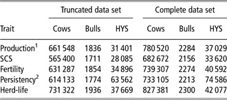
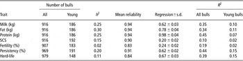
In the truncated data set, all records with freshening dates after September 2006, were deleted. The numbers of cows, bulls and HYSs included in the truncated and complete data sets for each trait are given in Table 1. Depending on the trait analyzed, there were 148 to 192 ‘young bulls’ with genotypes and EBVs based on daughter records in the complete data set, but without daughter records in the truncated data set. The number of bulls with genotypes and EBVs in the complete data set, and the number of young bulls with genotypes, but without EBVs in the truncated data set, are given in Table 2. Foreign bulls and bulls of breeds other than the Holstein were excluded, because these bulls do not accurately represent the Israeli Holstein population. Mean daughter deviations (MDD) per sire for the young bulls were computed as the weighted mean of sire's daughter records, with the appropriate HYS and parity effects subtracted from the phenotypic record. Means of cow records were weighted by n/(n + δ) where n is the number of records per cow and δ is the ratio of residual to cow effect variance. For milk production traits, δ = 1. MDD differ from DYD in that MDD are not corrected for merit of mates.
Numbers of cows, bulls and HYS included in the truncated and complete data sets for each trait

HYS = herd-year-seasons; SCS = somatic cell score.
1Numbers of animals and HYS were the same for milk, fat and protein production.
2Numbers of HYS were greater for persistency, because first and later parities were assigned to separate HYS.
Regressions of the EBV on the sum of their marker effect values

EBV = estimated breeding values; SCS = somatic cell score.
Selection of markers for inclusion in genomic evaluation
Significant linkage disequlibrium between SNP genotypes of the bulls and QTL for all 40 094 valid SNPs for all traits analyzed was estimated by the following regression model:

where EBVij is the breeding value of bull i for trait j, S the SNP genotype, BY the birth year and eij the random residual. Heterozygotes were scored as 1 and homozygotes as either 0 or 2.
For each trait, the 2000 SNPs with the lowest P-values for the effect of SNP genotype were reanalyzed individually by the MTC restricted maximum likelihood (REML) program, for the following model:

where Aij is the additive genetic effect of bull i for trait j, and the other terms are as described previously. The additive genetic and SNP effects were considered random variables in this analysis. The relationship matrix included all known parents and grandsirs of the bulls with genotypes. Although each individual has two parents and two grandsires, not all female ancestors were known, and nearly all the male ancestors were already included among the genotyped animals. Therefore, inclusion of these ancestors approximately doubled the number of animals included in the analysis. The allelic substitution effect was derived under the assumption of additivity from the following equation:

where rvj is the allelic substitution effect for trait j, σsj the square root of the SNP component of variance for trait j and ps the frequency of the less frequent marker allele in the population of bulls.
Significance values for the SNP component of variance were determined by permutation analysis. One thousand repeat analyses of a typical data set with randomization of the SNP effects relative to the bulls’ EBVs were run. The SNP component of variance was >2% of the total variance for <5% of the repeat samples. Thus, this criterion was used to determine significance of the marker effect.
Analysis methods and selection schemes
For each trait analyzed, the 400 markers with the greatest variance components for that trait were used for computation of GEBVs. Thus, a different set of markers were analyzed for each trait. Method I GEBVs for the young bulls were computed by the following algorithm:
1. For animals that were genotyped, we assumed that all genotypes were determined without error. Probabilities of genotypes for all other animals were computed based on the algorithm of Kerr and Kinghorn (Reference Kerr and Kinghorn1996). For animals with unknown parents, genotype probabilities were assumed to be equal to the mean probabilities in the entire sample of genotyped bulls.
2. The effects of these 400 markers were estimated jointly by the ‘cow model’ of Baruch and Weller (Reference Baruch and Weller2008).
3. The sum of the 400 marker effects as estimated by the cow model were subtracted from the production records of the cows based on each cow's genotype probabilities, and the marker effects as estimated by the cow model.
4. Multitrait AM evaluations were then computed for the adjusted records of the truncated data set. These EBVs are now based only on the effects not accounted for by the markers.
5. The GEBVs of the young bulls were computed as the parent average of the EBVs, which were computed from the adjusted records plus the sum of marker effects for each young bull.
The ‘cow model’ used to estimate the marker effects was as follows:

where Yijklmn is the record of cow n in parity k for trait i, Cin the random effect of cow n for trait i, qlm the inferred genotype probability l for marker m based on each cow's genotyped ancestors, rim the effect of marker m on trait i; and the other terms are as defined for equation (1). qlm were scored over the scale of 0 to 1, where 0 = homozygote for the ‘negative’ QTL allele and 1 = homozygote for the ‘positive’ QTL allele. Marker substitution effects were computed as 0.5rim. As only sires were genotyped, no female could have an inferred genotype of either 0 or 1. Covariances among the random cow effects are assumed to be zero. That is, the relationship matrix was not included. Although the cow effect includes the polygenic and the permanent environmental effects, it does not include the QTL effects. As the magnitude of these effects is not known, the cow model was first run under that assumption of QTL effects of zero. That is, the variance due to the cow effect is equal to 0.5 for milk production traits. Once estimates of the marker effects were obtained, the sum of the variances due to the marker effects were deleted from the cow effect as follows:

where  is the variance of the cow effect after subtraction of QTL effects,
 the variance of the cow effect including QTL effects, pm the estimated frequency of the less frequent allele for QTL i and rm the estimated substitution effect for QTL m. The cow model was run three times with estimates of
 updated at each iteration.
In Method II, regression coefficients were derived from the predictor bull population as follows:

where EBVijk is the EBV of bull j for trait i in the truncated data set, inti the y-intercept for trait i, MEBVij the mean of bull's parents EBV in the truncated data set for trait i, MSij the sum of marker scores for this bull for trait i, Bk the bull's birth year k, eijk the random residual, and a, b and c are regression coefficients. GEBVs for the young bulls were then derived from equation (7) using the y-intercept and regression constants obtained from the predictor bulls. As a was generally <1 and b was always <1, this method can be considered more ‘conservative’ than Method I, in that standard deviations among the evaluations were smaller. The GEBVs were also computed by the method of equation (1) in VanRaden (Reference VanRaden2008) for protein production (Method III). The dependent variable was the sires’ MDD, as described previously. Only 730 bulls with reliabilities >50 in the truncated data set were included. Residual variances were derived from the sires’ reliabilities, as described by VanRaden (Reference VanRaden2008). All 40 094 valid markers were included. The GEBVs were computed as Zû. The Zû for the young bulls were then computed based on the marker effects derived from the truncated data set.
The GEBVs by all three methods were compared with the current genetic evaluations for bias, computed as the difference in the means and regression of current EBVs on GEBVs. Correlations were also computed between the current evaluations and the three GEBV methods and parent averages computed from the truncated data set. Finally, correlations were computed between MDD, GEBV, parent averages and current EBV.
Results
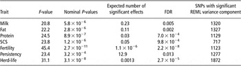
The F-values, the nominal P-values and the false discovery rate (FDR; Weller et al., Reference Weller, Song, Heyen, Lewin and Ron1998) values for the 50 SNPs with the lowest P-values by the regression model in equation (2) are given in Table 3 for the traits analyzed. All FDR values were ⩽0.1, and thus nearly all of these effects can be considered ‘real’ effects, unless the SNP effect is due to confounding with the polygenic effect due to relationships, as demonstrated by Habier et al. (Reference Habier, Fernando and Dekkers2007). Surprisingly, with the exception of persistency, there is an inverse relationship between the trait heritability and the FDR values; the higher the trait heritability, the lower the number of genes with detectable effects. From 717 (for SCS) to 1872 (for herd-life) of the 2000 effects with the lowest P-values by the linear model also had significant marker effects by the REML analyses. That is, the marker explained >2% of the variance. Thus, overall, more than half of the SNPs with the greatest effects by the regression model were also significant by the variance component model. The value for SCS was much lower than for the other traits. There was higher correspondence between the linear and REML models for the production traits, which had higher heritability. The correlations between the regression model F-values, derived from equation (2) and the SNP variance component derived from the 2000 REML analysis (equation (3)) were generally in the range of 0.2, but only 0.1 for protein (data not shown).
P-values and FDR levels for the 50 SNP effects with the lowest P-values for the traits analyzed

FDR = false discovery rates; SNP = single nucleotide polymorphism; REML = restricted maximum likelihood; SCS = somatic cell score.
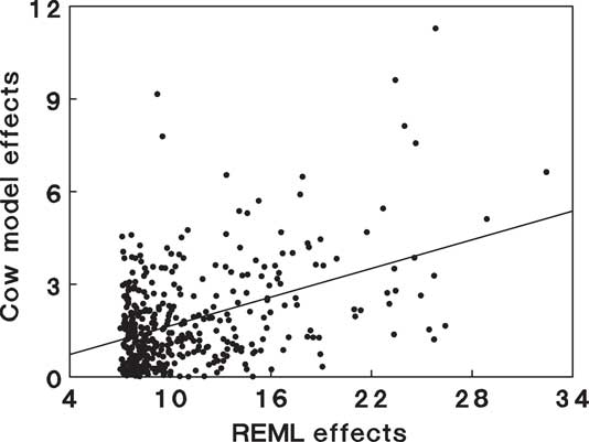
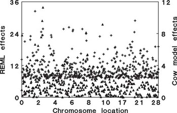
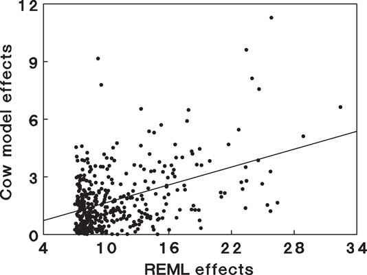
Comparison of SNP substitution effects for protein from the REML analysis (rvj, equation (4)) and the cow model (rim, equation (5)) are given in Figures 1 and 2. In Figure 1, the cow model effects are plotted as a function of the REML effects. The regression line is also plotted. As expected, the cow model effects are smaller because all the effects were included in the same analysis, whereas in the REML analyses each SNP was analyzed separately. The sum of the marker variances from the individual REML analyses explains more than 100% of the total sire variance. This is not surprising, as several markers may be linked to the same QTL. Furthermore, REML effects are biased upward. In addition, the SNP effects were considered random in the REML analysis and fixed in the cow model. Ramifications of whether these effects are considered fixed or random were considered in detail by Gianola et al. (Reference Gianola, de los Campos, Hill, Manfredi and Fernando2009). The correlation between the SNP effects for protein production from REML analysis was only 0.36. The SNP with the greatest effect in the cow model was ranked 15th by the REML analysis, and the SNP with the third largest effect by the AM was ranked 121th by the REML analysis.
The cow model substitution effects as a function of the restricted maximum likelihood substitution effects for kg protein. The regression line is also plotted.
Comparison of single nucleotide polymorphism substitution effects for protein from the restricted maximum likelihood (REML) analysis and the cow model ordered by chromosomal location. +, REML effects; ▴, cow model effects.

In Figure 2, SNP effects for protein from the REML analysis and the cow model are plotted by chromosomal location. Although one of the largest REML effects was found on Bos taurus chromosome (BTA) 6 near the location of ABCG2 (Cohen-Zinder et al., Reference Cohen-Zinder, Seroussi, Larkin, Loor, Wind, Lee, Drackley, Band, Hernandez, Shani, Lewin, Weller and Ron2005), this was not the case for the cow model effects. The largest REML effects were found on BTA1 and 20, although no major QTL affecting protein has been verified in these regions. The largest cow model effects were obtained on BTA2 and 10, also in regions not so far identified to harbor major protein QTL.
Regressions and R 2 of the EBVs of bulls with genotypes on the sum of their marker effect values are given in Table 2. All regressions were less than unity. The y-intercepts are also given in this table, but are to some extent arbitrary, because the directions of the marker effects estimated in the cow model were also arbitrary. The R 2 values ranged from 10% for SCS to 45% for protein production. The R 2 values tended to increase with increase in the regressions. There was no clear relationship between the R 2 values and the heritabilities. These results should be compared with the rather surprising results for human height. Despite the fact that height has a heritability of 0.8, effects from very large genome scans were able to explain only 5% of the variance (Maher, Reference Maher2008). The R 2 values are also presented for the young bulls with current EBVs, but without daughter records in the truncated data set. All R 2 values for the young bulls were <0.4 of the R 2 values for all bulls. A possible explanation is that QTL, with relatively large effects that were segregating in the population in previous years, reached fixation in the group of young bulls.
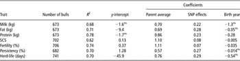
The R 2 values and regression coefficients derived from the truncated data set to compute the Method II GEBVs are given in Table 4 with their standard errors. Only bulls with dam EBVs based on at least one daughter record were included. The number of bulls ranged from 673 for production traits to 741 for herd-life. The y-intercepts were not significantly different from zero for milk and protein (P < 0.05). The effect of birth year was not significant for milk, fat, persistency and herd-life. The regressions of parent average and the sum of marker effects were significant for all traits (P < 0.001). The regression coefficients of the SNP effects were <0.3 for all traits, as compared with the Method I GEBVs, which assume coefficients of unity. The R 2 values ranged between 0.62 for SCS and 0.78 for protein.
Regression coefficients ± s.e. and R 2 used to derive the Method II GEBV

GEBV = genomic estimated breeding value; SNP = single nucleotide polymorphism; SCS = somatic cell score.
1ns, P < 0.05.
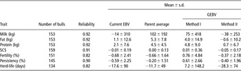
Means ± s.d. of current EBVs and GEBVs of the young bulls by trait are given in Table 5. For all three milk production traits, the parent averages were higher than the current EBVs. Thus, parent averages were biased upward. The classical explanation for this finding is preferential treatment of bull dams (e.g. Kuhn et al., Reference Kuhn, Freeman and Fernando1999). However, this should not be a major factor in Israel, where prices of bull calves are only slightly higher than the beef prices. One possibility is that most of the bull dams are the animals with the highest EBVs for milk production traits, and at the extreme ends of the population heritabilities are lower. Method I evaluations were also biased upward, but less so than the parent averages. Method II GEBVs were negatively biased for the milk production traits; however, in all cases the absolute value was less than for the parent averages and the Method I GEBVs. Bias for SCS was minimal for all three methods. Method I evaluations were biased upward for fertility, persistency and herd-life. Standard deviations were smallest for parent averages, as expected. Method I s.d. were the largest, and even larger than the current EBVs. Method II s.d. were between the parent averages and the current EBVs.
Means ± s.d. of current EBV, parent average EBV in the truncated data set and GEBV of the young bulls by trait

EBV = estimated breeding value; GEBV = genomic estimated breeding value; SCS = somatic cell score.
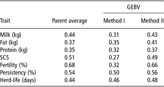
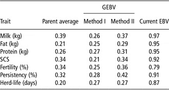
Correlations of current EBVs with parent averages and GEBVs of the young bulls by trait are given in Table 6. The correlations with the Method I GEBVs were lower than the parent averages and Method II GEBVs for all traits. Thus, Method II is clearly superior to Method I, both by the criteria of bias and accuracy. The correlations with Method II GEBVs were higher than the correlations with parent averages for fat, protein, persistency and herd-life.
Correlations of current EBV with parent average EBV and GEBV of the young bulls by traitFootnote 1

EBV = estimated breeding value; GEBV = genomic estimated breeding value; SCS = somatic cell score.
1 The numbers of young bulls by trait are given in Table 5.
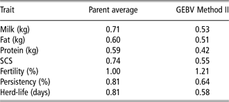
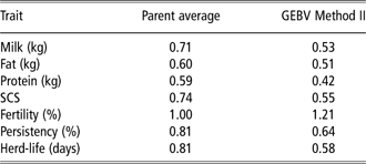
Regressions of current EBVs on parent averages, and Method II GEBVs of the young bulls by trait are given in Table 7. If the GEBVs are unbiased, regression should equal unity. All regression were <1.0, except for fertility. The regressions for parent averages were higher than the Method II regressions, except for fertility.
Regressions of current EBV on parent average EBV and Method II GEBV of the young bulls by traitFootnote 1
EBV = estimated breeding value; GEBV = genomic estimated breeding value; SCS = somatic cell score.
1 The numbers of young bulls by trait are given in Table 5.
The high parent average correlation for fertility may reflect the fact that mean reliability was lower for this trait, because of the heritability of only 2% in first parity. Therefore, the current evaluations are affected more by the parent contributions, which should increase the correlation with the parent average. The correlations of MDD with parent average, Method II GEBVs and current EBVs of the young bulls by trait are given in Table 8. Correlations of MDD with the milk production traits, SCS and persistency were between 0.91 and 0.97, but lower for fertility, which has very low heritability, and herd-life, which has only a single record per animal. Correlations of MDD with the Method II GEBVs were higher than the correlations of MDD with parent averages of all traits, except for milk and SCS, for which the two correlations were equal. The correlations of MDD with Method I were lower than the Method II correlations for all traits; however, Method I correlations were higher than the parent averages for fat, protein and herd-life.
Correlations of mean daughter record deviations with parent averages, GEBV and current EBV of the young bulls by traitFootnote 1

GEBV = genomic estimated breeding value; EBV = estimated breeding value; SCS = somatic cell score.
1 The numbers of young bulls by trait are given in Table 5.
The correlation between the sum of all marker effects from Method III analysis, Zû, and the EBVs of the bulls from the complete data set was 0.01, and was not significant. The correlation for the 186 bulls without daughter records in the truncated data set was −0.07, but also not significant. Thus, similar to the results of VanRaden et al. (Reference VanRaden, Van Tassell, Wiggans, Sonstegard, Schnabel, Taylor and Schenkel2009a) this method was not able to generate accurate GEBVs on a data set of this size. The standard deviation among Method III evaluations was only 2.14. This is apparently because of the small assumed variance of the individual marker effects, which were assumed to sum the total additive genetic variance (VanRaden, Reference VanRaden2008).
Discussion
Method II has the advantages as compared with the method of VanRaden (Reference VanRaden2008) in that the method of VanRaden (Reference VanRaden2008) is not effective for populations of this size, and genotypes of cows can be readily incorporated into Method II analysis without modification. Method II has the advantage over the method of Aguilar et al. (Reference Aguilar, Misztal, Johnson, Legarra, Tsuruta and Lawlor2010) in that computation of Method II GEBVs for new bulls with genotypes requires only calculation of a relatively simple regression equation, whereas the method of Aguilar et al. (Reference Aguilar, Misztal, Johnson, Legarra, Tsuruta and Lawlor2010) requires recalculation of the entire set of modified mixed model equations. An advantage of the method of Aguilar et al. (Reference Aguilar, Misztal, Johnson, Legarra, Tsuruta and Lawlor2010) is that the number of equations is independent of the number of markers. Thus, this method could also use all data from the high density SNP-chips with 777 000 markers.
Method II was superior to parent averages with respect to bias for production traits and persistency, and with respect to correlations with MDD for all traits, except for milk (which is not included in the Israel breeding index) and SCS. Unlike parent averages, Method II biases for production trait were negative. One of the main objections to insemination of cows with semen from young bulls with GEBVs is that, on an average, the genetic evaluations of these bulls tend to decrease when daughter records become available (e.g. http://www.altagenetics.com/English/Whatsnew/20101218Genomics.htm). This should not be the case for Method II EBVs.
Hayes et al. (Reference Hayes, Bowman, Chamberlain and Goddard2009) predicted that 5000 phenotypic records with genotypes should be required to obtain an accuracy of 0.6 for GEBVs with a heritability of 0.2. As heritability decreases, the number of genotypes required to reach the same accuracy increases. However, in this study, the highest correlation of Method II GEBVs with MDD was for persistency, even though this trait has moderate heritability.
VanRaden et al. (Reference VanRaden, Van Tassell, Wiggans, Sonstegard, Schnabel, Taylor and Schenkel2009a) obtained an R 2 value of 0.47 for protein between GEBVs and daughter deviations, as compared with an R 2 of 0.27 for the parent average. Both numbers were lower in this study. Their R 2 for net merit was 0.28 for GEBVs, compared with 0.11 for parent average; however, with only 1151 predictor bulls, the comparable numbers were 0.12 for GEBVs and 0.08 for parent average. This number of predictor bulls is still greater than the one in this study. In the analysis of the Holstein, Jersey and Brown Swiss populations by VanRaden et al. (Reference VanRaden, Wiggans, Sonstegard and Schenkel2009b) 4422, 1149 and 228 bulls, respectively, were included in the predictor samples. Gains in reliability for protein were 0 for Jerseys and 1% for Brown Swiss. Average gains were 11% for Jerseys, as compared with 29% for Holsteins. In 6 of the 24 traits analyzed, parent averages of Brown Swiss were more accurate than the GEBVs. In the most recent results from the United States, regressions of June 2010 daughter deviations on August 2006 genomic evaluations ranged between 0.51 and 0.62 for milk production traits for Brown Swiss, even though 1852 bulls were genotyped (Wiggans et al., Reference Wiggans, VanRaden and Cooper2011). The R 2 values ranged from 0.21 to 0.24. Thus, the method of VanRaden (Reference VanRaden2008) is clearly inefficient for analysis of populations of the relatively moderate size analyzed in this study.
The relatively low correlation between the REML effects and the cow model effects was rather surprising. This also tends to indicate that some SNPs with potentially large effects by the cow model were excluded from the analysis. Reasons for the relatively low correlation are: first, that REML variance components for samples of this size ('1000 animals with genotypes and '1150 ancestors) have relatively large confidence intervals; second, as SNPs on the same chromosome are correlated, the effects are reduced if multiple SNPs are included in the same analysis, relative to the situation in which each SNP is analyzed separately. Furthermore, if two SNPs are highly correlated, then attribution of the effect associated with both markers is virtually arbitrary, or dependent on allelic frequencies. Finally, in the REML analysis, each bull was weighted equally, whereas in the cow model the effects were determined based on the actual phenotypic records.
Weigel et al. (Reference Weigel, de los Campos, González-Recio, Naya, Wu, Long, Rosa and Gianola2009) compared GEBVs of net merit computed with all valid SNP markers to GEBVs computed with subsets of markers. The R 2 for the complete marker set was 0.375. The R 2 values for subsets of the 300, 500, 750, 1000, 1250, 1500 and 2000 SNPs with largest effects were 0.184, 0.236, 0.279, 0.289, 0.307, 0.313 and 0.322, respectively. Increasing the number of SNPs over the range of 10 000 to 40 000 increased the R 2 values generally by only 2% to 4% (VanRaden et al., Reference VanRaden, Van Tassell, Wiggans, Sonstegard, Schnabel, Taylor and Schenkel2009a).
Inclusion of all the markers in the method presented is not yet a viable option, because of computing limitations; however, the number of markers could be increased if the additional gain in computing time is economically justified. With respect to computing time, the limiting factor is iteration of the cow model, which required close to 24 h for completion of 2000 iterations on a HP BL860C single processor server blade. Although addition of 400 marker equations does not significantly increase the total number of equations, the cow by marker sub-matrix has no empty cells. Therefore, running time for the cow model is more than double the run time for the multitrait AM, in which the vast majority of cells in the coefficient matrix are empty.
Reducing the number of markers in the current analysis from 400 to 300 reduced R 2 of current EBVs on the sum of marker effects for protein from 0.45 to 0.24. The correlation of GEBVs with current EBVs was not reduced; however, the correlation of GEBVs with MDD was reduced from 0.31 to 0.29. Thus, a moderate increase in the number of markers included in the Method II analysis apparently will not result in a substantial improvement, at least for traits with intermediate heritability.
Conclusions
A method for marker-assisted selection based on genotype probabilities for animals that were not genotyped is presented. Correlations by Method II GEBVs were higher than the correlations with the parent averages for fat and protein production, milk production persistency and herd-life. Method II GEBVs were less biased than parent averages for milk production traits. Increasing the number of markers included in the analysis should marginally increase the accuracy of the evaluations, at least for milk production traits.
Acknowledgments
This research was supported by grants from the Israel milk marketing board, the European Sixth Research and Technological Development Framework Programme, Proposal no. 016250-2 SABRE, and Binational Agricultural Research and Development Fund (BARD) Research Project IS-4394-11R. Genotyping was performed by A. Schein and N. Avidan, Pharmacogenetics and Translation Medicine Center, the Rappaport Institute for Research in the Medical Sciences, Technion, Haifa, Israel, and GeneSeek, Lincoln, NE.