



1. Introduction
In general, thrust in a flapping propulsor is a consequence of the momentum imparted to the flow by the transversely moving solid boundary. In flexible flapping propulsors, one conjectures that thrust and propulsive efficiency are consequences of the interplay between the elastodynamics of the flexible solid and vorticity dynamics of the fluid. It is important to remember that the elastic deforming solid is a moving boundary to the fluid flow, and the consequent fluid pressure a distributed time-varying forcing on the elastic solid, and that there is a feedback relation between the two.
In the past, numerical and experimental studies on flexible foil flapping propulsion have revealed a variety of fluid–elastic behaviour. There have been studies on flexible foils where the flexible foil has been attached to the trailing edge of a rigid airfoil to prevent leading-edge vortex formation over the flexible foil, and then there are investigations that study the influence of aspect ratio on thrust and propulsive efficiency. These investigations, important no doubt, have very little bearing on the problem that we address here.
Here, we are concerned with vortex formation, transport and their structure in relation to the elastodynamics of the flexible flapper in a two-dimensional flow; the interplay of flexible foil motion variables and fluid pressure on thrust and power input to the foil along its length; and thrust and propulsive efficiency variation in relation to various scaling parameters. So our review of the literature is restricted to these topics.
Recently, Quinn, Lauder & Smits (Reference Quinn, Lauder and Smits2014), presented results for heaving a flexible flat plate in a fluid at Reynolds numbers in the range 7800–46 000. They observe thrust peaks that coincide with frequencies where the trailing-edge amplitude is a local maximum. The time-averaged thrust varies parabolically with Strouhal number. The scaled propulsive efficiency
 ${\it\eta}St$
too peaks at almost the same frequencies where the thrust maxima occur, and progressively increase with the scaled frequency parameter.
An obvious and recurring problem of interest is the thrust and propulsive efficiency of flexible foils in relation to a rigid one. A number of studies address this. Formation of a leading-edge vortex, and its separation, occurs for large amplitude pitching of rigid airfoils. Marais et al. (Reference Marais, Thiria, Wesfreid and Godoy-Diana2012) have shown that the symmetry breaking of the vortex wake seen in a pitching rigid foil was suppressed in a flexible foil, and larger trailing-edge deflections result in three times more thrust than for a rigid airfoil for the same pitching amplitude. They also correlate the separation distance within a vortex pair with wake deflection or symmetry breaking. Thiria & Godoy-Diana (Reference Thiria and Godoy-Diana2010) have shown that flexible wings generate more thrust more efficiently than rigid wings, and that the thrust and input power scale linearly in terms of a parameter that is the ratio of wing inertia to its flexibility. It is known that thrust and efficiency maxima occur at a set of discrete frequencies close to the in-vacuum natural frequencies of the solid (Michelin & Smith Reference Michelin and Smith2009). Partially flexible and heavier foils were shown to be more efficient in generating thrust, and the vorticity contours of lighter foils were distinct from the heavier ones (Pederzani & Haj-Hariri Reference Pederzani and Haj-Hariri2006). In another study, by Prempraneerach, Hover & Triantafyllou (Reference Prempraneerach, Hover and Triantafyllou2003), using water tunnel experiments, flexible airfoils oscillating in heave and pitch were shown to be 36 % more efficient than a rigid airfoil, with almost no change in thrust; the thrust coefficient increased with Strouhal number
 $2h_{0}\,f/U$
for a given value of flexibility. Ignoring the influence of inertia but coupling the elasticity of the solid with the fluid dynamics, Katz & Weihs (Reference Katz and Weihs1978) showed that flexible foils are more efficient in generating thrust though the thrust levels are lower relative to rigid foils. Modelling the influence of flexibility as a travelling wave, thrust was shown to increase, and propulsive efficiency decrease, with reduced frequency, in a one-dimensional flexible solid immersed in a two-dimensional incompressible potential flow (Wu Reference Wu1961). Earlier, Lighthill (Reference Lighthill1960) showed that thrust can be generated by travelling waves in a slender body of revolution in a potential flow only when its phase velocity is greater than
 $5/4$
th the forward speed.
The generation and transport of vorticity by a flexible undulating solid is in fact discussed quite extensively in the literature concerned with the locomotion of aquatic animals. We restrict our interest to anguilliform locomotion, and even though the numerical simulations refer to a three-dimensional flow field, we think some of the results and findings may have relevance to the problems of interest to us here. Efficient swimming of anguilliform swimmers involves substantial lateral displacements from the mid-body to the tail that contribute to thrust (Kern & Koumoutsakos Reference Kern and Koumoutsakos2006). Vorticity patterns from their computational fluid dynamic simulations on anguilliform swimming seem to qualitatively agree with those of experiments on live eel. Experimental measurements of flow velocity and body undulations on live eel (Müller et al. Reference Müller, Smit, Stamhuis and Videler2001) correlate vorticity with body kinematics; the flow speed adjacent to the body increases linearly along its length and the authors conjecture that this is suggestive of thrust being generated throughout the body. Carling, Williams & Bowtell (Reference Carling, Williams and Bowtell1998) have correlated the net force with time-varying streamline patterns of an undulating one-dimensional flexible solid model of an eel in a two-dimensional incompressible viscous flow using numerical simulations. The ratio of wavespeed to forward speed of the swimmer that they computed – 0.77 – comes within the range predicted by Lighthill (Reference Lighthill1960) for thrust generation.
In related studies on rigid airfoils oscillating transversely to the free stream, the wake and vorticity over the rigid foil were correlated with thrust and efficiency and there is now some understanding of the mechanisms that generate thrust. At low frequencies of oscillation in heave, frequencies and amplitudes for which the leading-edge vortex remains attached and convects on the surface of the foil reinforcing the trailing edge vortex generate large thrust (Wang Reference Wang2000). The amplitude and frequency dependence on the formation, growth and transport of the leading-edge vortex, as well as the nature of the vortex wake, has been catalogued by Lewin & Haj-Hariri (Reference Lewin and Haj-Hariri2003). The motion of the leading-edge vortex and the wake are correlated with the output and input power and efficiency.
Here, we are mainly concerned with understanding what causes high thrust and efficiency, or drag, in terms of the motion of the elastic solid and the vortex wake around it; the spatio-temporal evolution of slope, curvature, velocities and accelerations of the foil are correlated with vorticity and pressure around the foil. The role of circulatory and non-circulatory forces on thrust, both spatially over the foil and as a function of time, their relationship to the foil kinematics, and consequent influence on thrust and propulsive efficiency, are clearly defined. Phase relations between pressure and inertial forces and foil motion clearly demarcate the drag or thrust generating regions, and propulsive efficiency. The foil is modelled as a one-dimensional elastic solid; a Bernoulli–Euler beam vibrating in flexure with sinusoidal forcing at its fixed end. The fluid flow is two-dimensional, viscous and incompressible.
The results and analysis presented here are arranged as follows. In § 2, we discuss the fluid–elastic model along with its numerical implementation. Section 3 presents results on thrust, propulsive efficiency, flapping velocity and other parameters, for the complete frequency range for which we numerically simulated the fluid–elastic system. Section 4 then interrogates the vorticity, phase relationships, kinematics of the foil and its influence on thrust and propulsive efficiency, in three distinct frequency regimes of the complete frequency range. Section 5 is an exercise in correlating thrust along the foil length with fluid flow velocity close to the foil surface for the three thrust maxima frequencies. The variation of thrust and propulsive efficiency as a function of trailing-edge Strouhal number is discussed in § 6. We conclude by summarizing the results presented here and their significance.
2. The fluid–elastic model
The fluid model is a two-dimensional incompressible viscous flow and the solid a Bernoulli–Euler one-dimensional model of flexure, as shown in figure 1. Given the flight speeds occurring in natural flapping wing propulsors, the assumption of incompressibility is justified. Two-dimensionality of the flow physics is however a restrictive assumption as most flows of interest pertaining to flapping propulsion are likely to have spanwise variations. Nevertheless, it keeps the problem simple and allows us to focus on understanding the influence of elasticity, inertia and vorticity on propulsion.
The numerical implementation of the fluid dynamics uses a sharp-interface immersed-boundary technique and the Bernoulli–Euler solid model is discretized using finite elements. Their dynamics are loosely coupled using a predictor–corrector algorithm.
Flexible foil in a fluid flow.
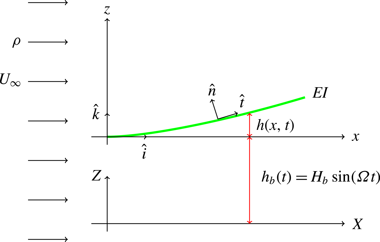
The equation of motion of the flexible foil is the Bernoulli–Euler model of a one-dimensional elastic solid in flexure (Clough & Penzien Reference Clough and Penzien1993, chap. 17)
 $$\begin{eqnarray}m\frac{\partial ^{2}h(x,t)}{\partial t^{2}}+c\frac{\partial ^{5}h(x,t)}{\partial t\partial x^{4}}+EI_{yy}\frac{\partial ^{4}h(x,t)}{\partial x^{4}}={\rm\Delta}p(x,t)\hat{\boldsymbol{n}}\boldsymbol{\cdot }\hat{\boldsymbol{k}}-m\frac{\text{d}^{2}h_{b}(t)}{\text{d}t^{2}};\quad 0<x<L.\end{eqnarray}$$
The boundary conditions for the cantilever beam are the no-displacement and no-slope condition at the fixed end, and no-shear force and no-bending moment at the free end. Each term in (2.1) has the dimensions of pressure since we are considering a spanwise section of the foil to comply with the assumption of two-dimensional fluid dynamics.
 $h(x,t)$
is the elastic transverse deflection of the beam in flexure,
 $m$
is the mass per unit length per unit span of the foil,
 $EI_{yy}$
is the flexural rigidity per unit span of the foil with
 $E$
denoting Young’s modulus of the material of the foil and
 $I_{yy}$
is its sectional second moment of area per unit span about the
 $y$
axis of the coordinate system attached to the beam,
 $c$
is the damping coefficient per unit span of the material of the beam based on a model wherein the damping force induced in the material of the beam due to vibration is proportional to the strain rate,
 ${\rm\Delta}p(x,t)$
is the pressure differential across the top and bottom surface of the foil due to the unsteady fluid flow on the beam,
 $\hat{\boldsymbol{n}}$
is the vector denoting the normal to the upper surface of the foil and
 $h_{b}(t)$
is the harmonic base excitation applied at the cantilevered end of the beam, and is defined in the present case, without loss of generality, as
 $h_{b}(t)=H_{b}\sin {\it\Omega}t$
.
The assumptions that underlie the Bernoulli–Euler model of flexure involve small amplitudes of oscillation relative to the length of the foil, small values of slope and curvature and low frequencies of oscillation. In our discussion of the results we will have occasion to review some of these restrictions.
The pressure differential
 ${\rm\Delta}p(x,t)$
over the foil is determined using the incompressible Navier–Stokes model of the fluid flow. The normal component of the viscous force –
 $2{\it\mu}(\partial u_{n}/\partial x_{n})\hat{\boldsymbol{n}}$
– is small relative to the pressure force so that we neglect it altogether. In fact, as we will show in our analysis, even the tangential component of the viscous force is small relative to the pressure force. However, viscosity significantly affects the structure and transport of vorticity.
Incompressibility of the fluid is justified since the flow speed in almost all cases of flying or swimming animals is below Mach
 $0.3$
and therefore one can safely assume that compressibility effects are not significant.
The governing equations of the fluid dynamics is given by
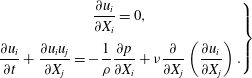 $$\begin{eqnarray}\left.\begin{array}{@{}c@{}}\displaystyle \frac{\partial u_{i}}{\partial X_{i}}=0,\\ \displaystyle \frac{\partial u_{i}}{\partial t}+\frac{\partial u_{i}u_{j}}{\partial X_{j}}=-\frac{1}{{\it\rho}}\frac{\partial p}{\partial X_{i}}+{\it\nu}\frac{\partial }{\partial X_{j}}\left(\frac{\partial u_{i}}{\partial X_{j}}\right).\end{array}\right\}\end{eqnarray}$$
Note that the fluid dynamical variables are defined in a laboratory fixed inertial frame of reference
 $X_{i}$
, that is distinct from the coordinate system that defines the foil displacement
 $x,z$
which is fixed to the leading edge of the foil and hence moving with it.
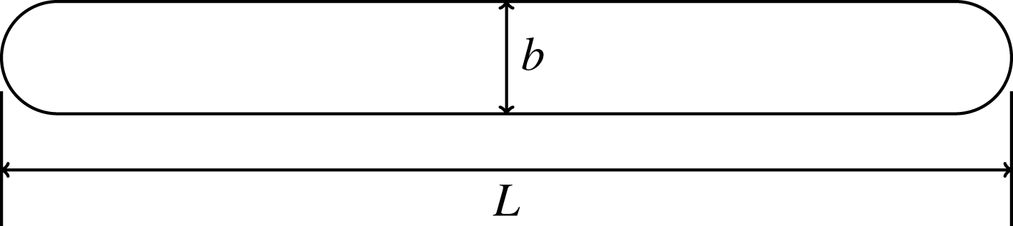
The geometry of the foil is shown in figure 2. The foil thickness
 $b$
is 4 % of the length
 $L$
of the foil and its leading and trailing edge are circular.
Geometry of the foil.
The fluid flow equations are solved numerically using a cell centred and collocated arrangement for the component velocities
 $u_{i}$
and the pressure
 $p$
in a non-uniform Cartesian grid defined in the Cartesian space
 $X_{i}$
along with temporal variable
 $t$
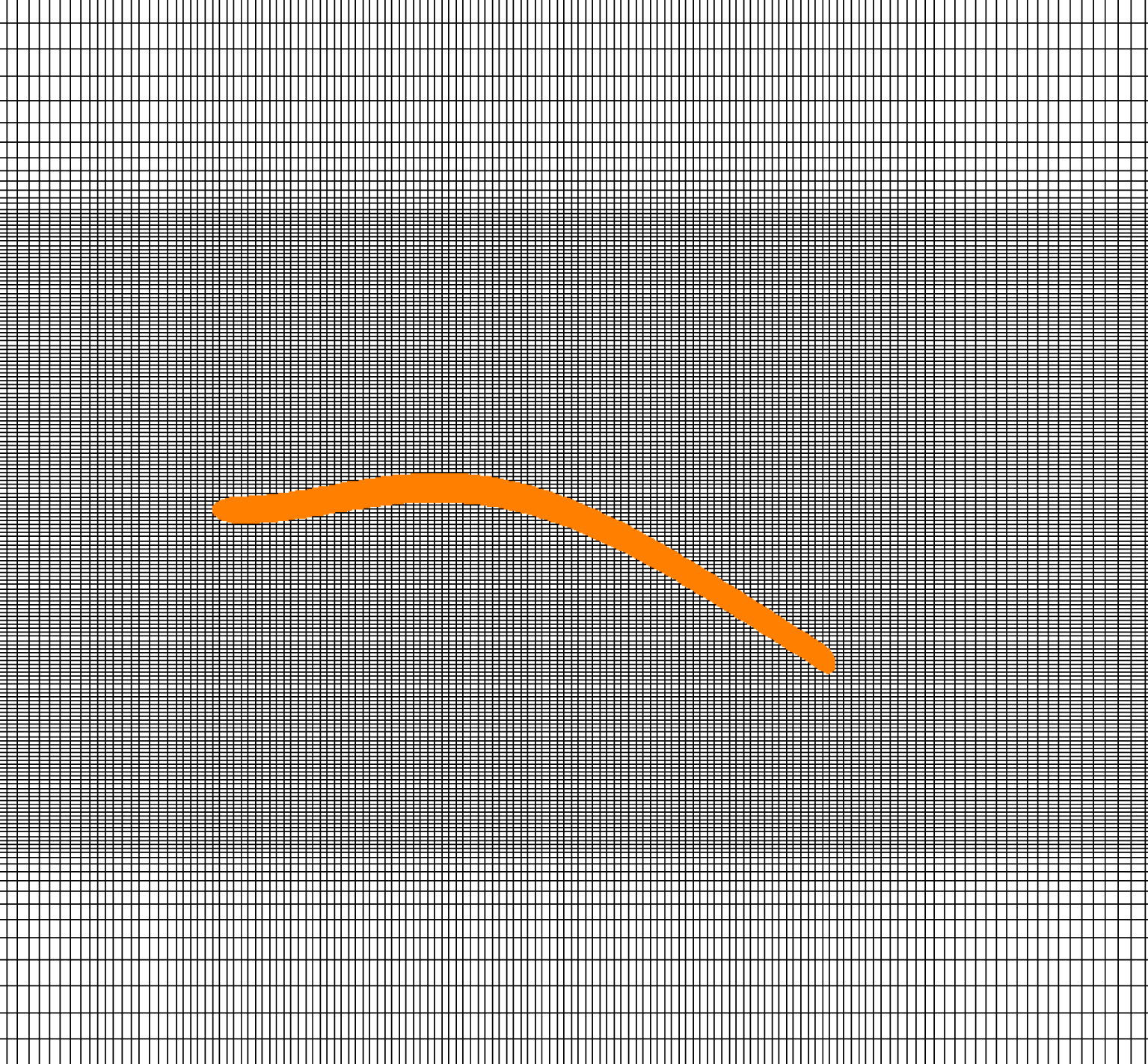
. A non-uniform Cartesian grid is used in which the body with the complex boundary of interest is placed as shown in figure 3. The governing equations are solved using the fractional step method of Kan (Reference van Kan1986). The first substep solves a modified momentum equation numerically that is used in evaluating the fluid velocities. The convective terms are discretized using a second-order Adams–Bashforth scheme and the diffusive terms are implicitly discretized using a Crank–Nicolson scheme. The second substep requires the solution of the pressure correction equation leading to the Poisson equation. A Dirichlet boundary condition is applied to solve the modified momentum equation and a Neumann boundary condition for the pressure Poisson equation. The boundary conditions near the immersed boundary are applied using the sharp interface procedure (Mittal et al.
Reference Mittal, Dong, Bozkurttas, Najjar, Vargas and von Loebbecke2008). The discretized momentum equation is solved using the Gauss–Sidel point-by-point iteration. The pressure Poisson equation is solved using preconditioned Bi-CGSTAB, a Krylov subspace based method. Stone’s implicit pre-conditioner (Ferziger & Peric Reference Ferziger and Peric2002) is used for the Poisson equation solver. As the convection term is treated explicitly, the time marching problem is restricted by the CFL number criteria.
Immersed boundary grid.
The coupled elastodynamic equation (2.1) is solved using finite elements (Clough & Penzien Reference Clough and Penzien1993, chap. 10). The pressure calculated from the viscous flow solver is used in the finite element based structural solver. At a given instant of time, the Lagrangian centre point of the finite element of the foil is surrounded by Eulerian grid points characterized as fluid nodes and ghost nodes. At every time step, after the flow solver computes the pressure at the Eulerian nodes, the pressure at the Lagrangian centre point of the finite element is interpolated from the values of the pressure at the surrounding nodes of the Eulerian grid. This value of pressure calculated at the centre of the finite element is assumed to be constant along the finite element. The flow solver was validated with steady, unsteady and moving boundary results from the literature. These results, together with the details on the immersed boundary method, computational grid and fluid–elastic coupling are presented in appendix A.
Rather than numerically integrating the dimensional equations, we rescale constants and variables that appear in the equations. One reason to do this is to reduce the number of parameters that can be independently varied. The other, and perhaps more important reason, is that we then have an idea of the relative magnitude of the various physical quantities used in the model. Time is rescaled as
 ${\it\tau}=t{\it\omega}_{c}$
where
 ${\it\omega}_{c}=\sqrt{EI/(mL^{4})}$
can be interpreted as a dynamic stiffness parameter for the foil. In a similar way, we non-dimensionalize the base excitation frequency
 $\bar{{\it\Omega}}={\it\Omega}/{\it\omega}_{c}$
. The spatial coordinates
 $x,{\it\xi}$
are rescaled with reference to the length of the foil
 $\bar{x}=x/L$
. Similarly, the foil flexural response is non-dimensionalized as
 $\bar{h}=h/L$
. The fluid free-stream speed is rescaled as
 $\bar{U}_{\infty }=U_{\infty }/({\it\omega}_{c}L)$
. The mass ratio
 ${\it\mu}=m/{\it\rho}L$
. The strain rate dependent material damping parameter
 $c$
is rescaled in terms of the dynamic stiffness and flexural stiffness –
 $\bar{c}=c{\it\omega}_{c}/(EI)$
– and its numerical value is so chosen such that the damping ratio in the first mode of vibration, in vacuum, is 1 % or
 $0.01$
. The base excitation displacement amplitude is rescaled as
 $\bar{H}_{b}=H_{b}/L$
. The non-dimensional velocity amplitude is then
 $\bar{{\it\Omega}}\bar{H}_{b}$
and in this study we have set
 $\bar{{\it\Omega}}\bar{H}_{b}=1$
.
The governing equation of the elastic Bernoulli–Euler one-dimensional solid in flexure, in non-dimensional form, is given by
 $$\begin{eqnarray}\frac{\partial ^{2}\bar{h}(\bar{x},{\it\tau})}{\partial {\it\tau}^{2}}+\bar{c}\frac{\partial ^{5}\bar{h}(\bar{x},{\it\tau})}{\partial {\it\tau}\partial \bar{x}^{4}}+\frac{\partial ^{4}\bar{h}(\bar{x},{\it\tau})}{\partial \bar{x}^{4}}=\frac{\bar{U}_{\infty }^{2}}{{\it\mu}}{\rm\Delta}\bar{p}(\bar{x},{\it\tau})\hat{\boldsymbol{n}}\boldsymbol{\cdot }\hat{\boldsymbol{k}}-\frac{\text{d}^{2}\bar{h}_{b}({\it\tau})}{\text{d}{\it\tau}^{2}};\quad 0<\bar{x}<1,{\it\tau}>0.\end{eqnarray}$$
Here
 $\bar{U}_{\infty }=U_{\infty }/({\it\omega}_{c}L)$
and
 ${\rm\Delta}\bar{p}={\rm\Delta}p/({\it\rho}U_{\infty }^{2})$
. The non-dimensional fluid dynamic equations then take the form
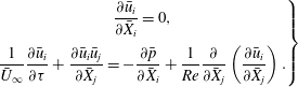 $$\begin{eqnarray}\left.\begin{array}{@{}c@{}}\displaystyle \frac{\partial \bar{u}_{i}}{\partial \bar{X}_{i}}=0,\\ \displaystyle \frac{1}{\bar{U}_{\infty }}\frac{\partial \bar{u}_{i}}{\partial {\it\tau}}+\frac{\partial \bar{u}_{i}\bar{u}_{j}}{\partial \bar{X}_{j}}=-\frac{\partial \bar{p}}{\partial \bar{X}_{i}}+\frac{1}{Re}\frac{\partial }{\partial \bar{X}_{j}}\left(\frac{\partial \bar{u}_{i}}{\partial \bar{X}_{j}}\right).\end{array}\right\}\end{eqnarray}$$
The Reynolds number is defined with reference to the length of the foil
 $L$
; that is
 $Re=U_{\infty }L/{\it\nu}$
, where
 ${\it\nu}$
is the dynamic viscosity of the fluid. The Reynolds number is set at a value of
 $1000$
for all the simulations presented here.
 $\bar{X}_{i}=X_{i}/L$
.
3. Thrust and propulsive efficiency
Thrust is a response of the fluid–elastic system to a time-varying input. Here this input is a sinusoidal forcing at the root or leading edge of the foil that is clamped. Thus energy is added to the fluid–elastic system through the base excitation. The thrust generated by the fluid–elastic system is parallel to the free stream. The contribution to thrust comes from the fluid pressure acting normal
 $\hat{\boldsymbol{n}}$
to the foil and the viscous force acting tangential
 $\hat{\boldsymbol{t}}$
to the foil, as shown in figure 1. Note that these force components have the dimensions of pressure as they are the force per unit span per unit length along the foil:
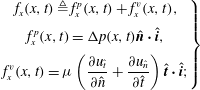 $$\begin{eqnarray}\left.\begin{array}{@{}c@{}}\displaystyle f_{x}(x,t)\triangleq f_{x}^{p}(x,t)+f_{x}^{v}(x,t),\\ \displaystyle f_{x}^{p}(x,t)={\rm\Delta}p(x,t)\hat{\boldsymbol{n}}\boldsymbol{\cdot }\hat{\boldsymbol{i}},\\ \displaystyle f_{x}^{v}(x,t)={\it\mu}\left(\frac{\partial u_{\hat{t}}}{\partial \hat{n}}+\frac{\partial u_{\hat{n}}}{\partial \hat{t}}\right)\hat{\boldsymbol{t}}\boldsymbol{\cdot }\hat{\boldsymbol{i}};\end{array}\right\}\end{eqnarray}$$
 ${\it\mu}$
is the coefficient of viscosity of the incompressible fluid. The respective force coefficients were then determined by integrating the pressure and viscous force components in the horizontal direction along the foil length and then dividing by
 $1/2{\it\rho}U_{\infty }^{2}L$
:
 $$\begin{eqnarray}\left.\begin{array}{@{}c@{}}\displaystyle C_{x}^{p}(t)=\frac{1}{1/2{\it\rho}U_{\infty }^{2}L}\int _{0}^{L}f_{x}^{p}(x,t)\,\text{d}x,\\ \displaystyle C_{x}^{v}(t)=\frac{1}{1/2{\it\rho}U_{\infty }^{2}L}\int _{0}^{L}f_{x}^{v}(x,t)\,\text{d}x,\\ \displaystyle C_{x}(t)=\frac{1}{1/2{\it\rho}U_{\infty }^{2}L}\int _{0}^{L}f_{x}(x,t)\,\text{d}x.\end{array}\right\}\end{eqnarray}$$
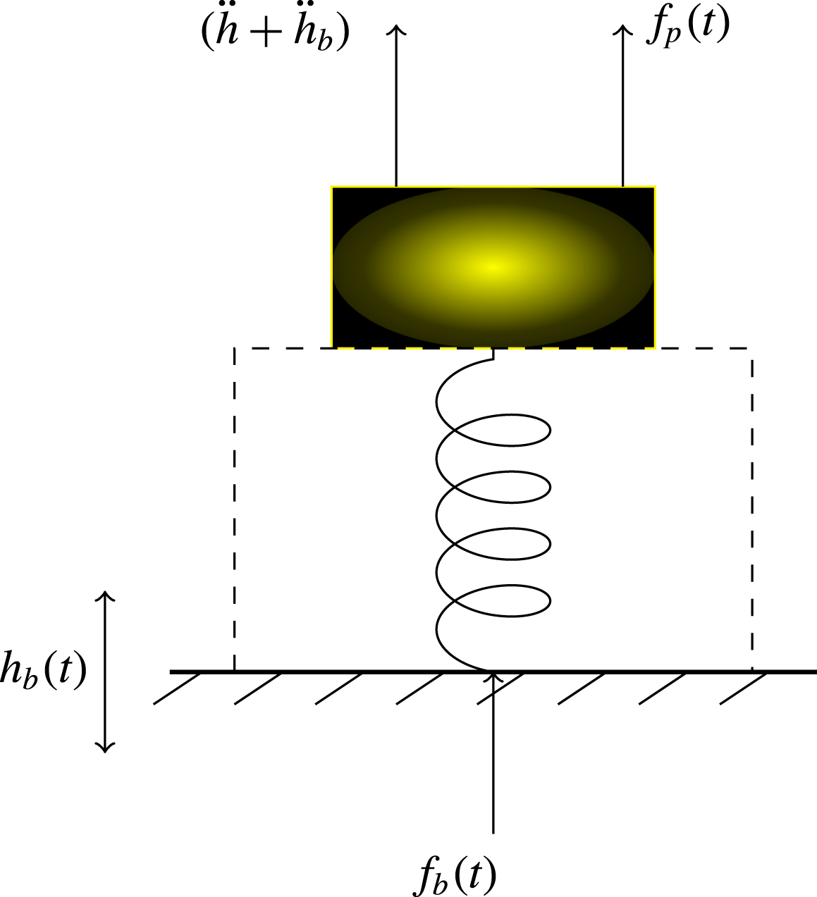
Input force
 $f_{b}(t)$
on the fluid–elastic system.
The propulsive efficiency of the oscillating fluid–elastic system is the ratio of the output power to the input power. The power input to this fluid–elastic system is the input force times the base excitation velocity. That is
 $P_{in}(t)=f_{b}(t){\dot{h}}_{b}(t)$
. The input force
 $f_{b}(t)$
is derived from dynamic equilibrium as shown in figure 4. Analytically
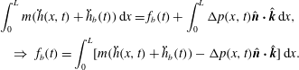 $$\begin{eqnarray}\displaystyle & & \displaystyle \int _{0}^{L}m(\ddot{h}(x,t)+\ddot{h}_{b}(t))\,\text{d}x=f_{b}(t)+\int _{0}^{L}{\rm\Delta}p(x,t)\hat{\boldsymbol{n}}\boldsymbol{\cdot }\hat{\boldsymbol{k}}\,\text{d}x,\nonumber\\ \displaystyle & & \displaystyle \quad \Rightarrow ~f_{b}(t)=\int _{0}^{L}[m(\ddot{h}(x,t)+\ddot{h}_{b}(t))-{\rm\Delta}p(x,t)\hat{\boldsymbol{n}}\boldsymbol{\cdot }\hat{\boldsymbol{k}}]\,\text{d}x.\end{eqnarray}$$
The power input is therefore
 $$\begin{eqnarray}P_{in}(t)=f_{b}(t){\dot{h}}_{b}(t)={\dot{h}}_{b}(t)\int _{0}^{L}[m(\ddot{h}(x,t)+\ddot{h}_{b}(t))-{\rm\Delta}p(x,t)\hat{\boldsymbol{n}}\boldsymbol{\cdot }\hat{\boldsymbol{k}}]\,\text{d}x.\end{eqnarray}$$
The output power is the thrust force times the forward velocity of the foil. The forward velocity of the foil is the free-stream velocity of the fluid flowing past the clamped oscillating foil. Therefore
 $$\begin{eqnarray}P_{out}(t)=f_{x}(t)U_{\infty }.\end{eqnarray}$$
The work output in one time period of the base excitation is then
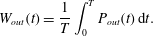 $$\begin{eqnarray}W_{out}(t)=\frac{1}{T}\int _{0}^{T}P_{out}(t)\,\text{d}t.\end{eqnarray}$$
The propulsive efficiency is defined (Lighthill Reference Lighthill1960) as the ratio of the output work to the input work. That is
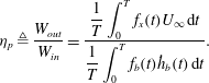 $$\begin{eqnarray}{\it\eta}_{p}\triangleq \frac{W_{out}}{W_{in}}=\frac{\displaystyle \frac{1}{T}\int _{0}^{T}f_{x}(t)U_{\infty }\,\text{d}t}{\displaystyle \frac{1}{T}\int _{0}^{T}f_{b}(t){\dot{h}}_{b}(t)\,\text{d}t}.\end{eqnarray}$$
The thrust coefficient is defined as
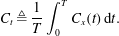 $$\begin{eqnarray}C_{t}\triangleq \frac{1}{T}\int _{0}^{T}C_{x}(t)\,\text{d}t.\end{eqnarray}$$
While computing thrust one needs to choose a flow speed at which there is no occurrence of flutter – a fluid-elastodynamic instability. Flow speeds where flutter occurs are to be avoided as the response to any kind of forcing at these flow speeds is likely to be unbounded or large and generate drag. At a flow speed of
 $\bar{U}_{\infty }=1$
there was no occurrence of large or unbounded amplitude response in the range of mass ratios and excitation frequencies chosen. Three mass ratios
 ${\it\mu}$
–
 $0.33$
,
 $0.2$
and
 $0.1$
– are chosen for the study. The excitation frequency range
 $\bar{{\it\Omega}}$
is between
 $0\rightarrow 60$
.
Thrust
 $C_{t}$
(a), efficiency
 ${\it\eta}_{p}$
(b), foil trailing-edge velocity (c), and trailing-edge angle of incidence (d) as a function of excitation frequency for different mass ratios.
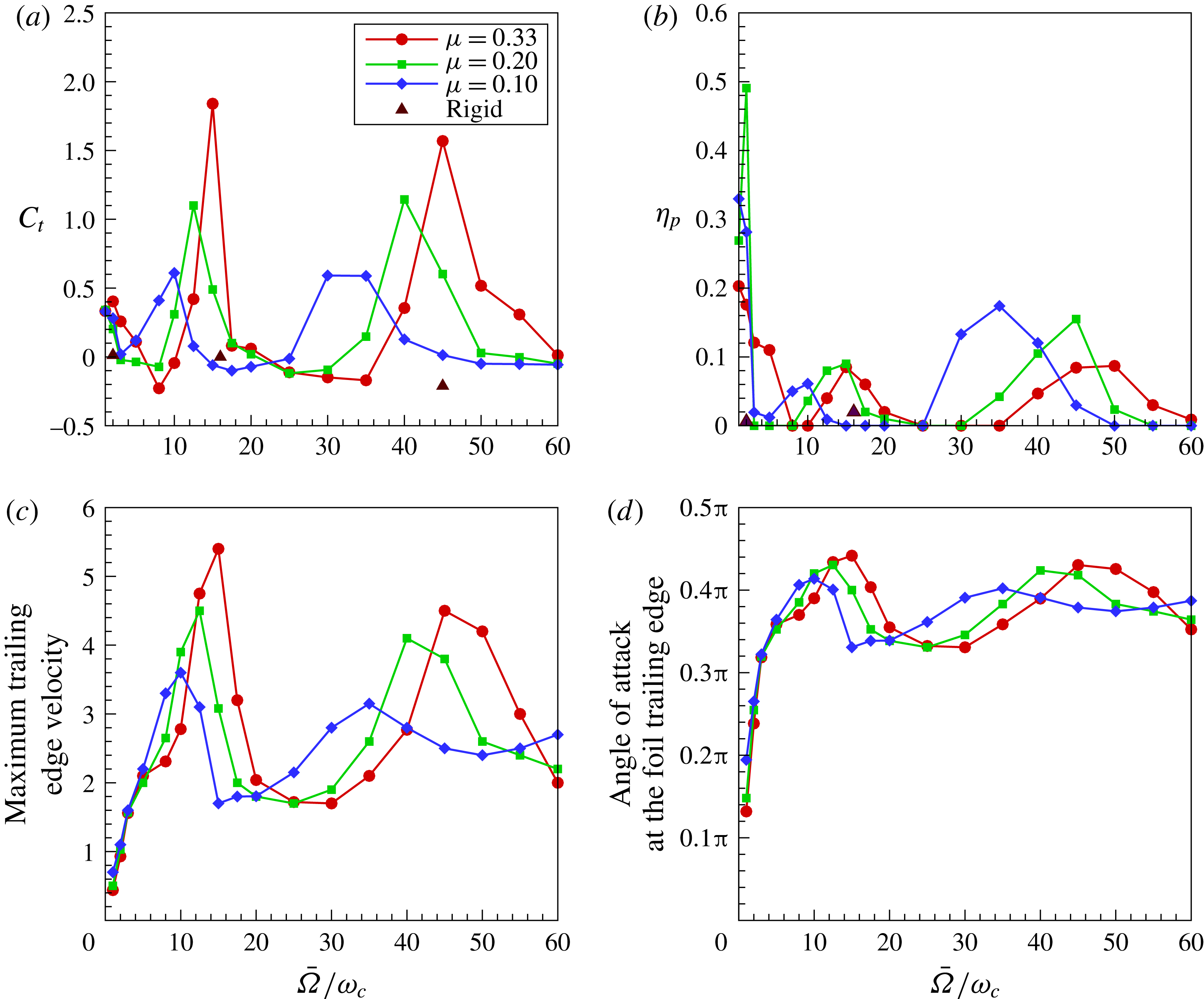
Figure 5 shows the variation of thrust coefficient, propulsion efficiency, foil trailing-edge velocity
 $\partial \bar{h}_{t}/\partial {\it\tau}$
and trailing-edge angle of incidence
 ${\it\alpha}_{t}=(1/\bar{U}_{\infty })(\partial \bar{h}_{t}/\partial {\it\tau})+(\partial \bar{h}_{t}/\partial \bar{x})$
, at various excitation frequencies for different mass ratios of
 $0.33$
,
 $0.2$
and
 $0.1$
. The excitation frequency range covers
 $0\rightarrow 60$
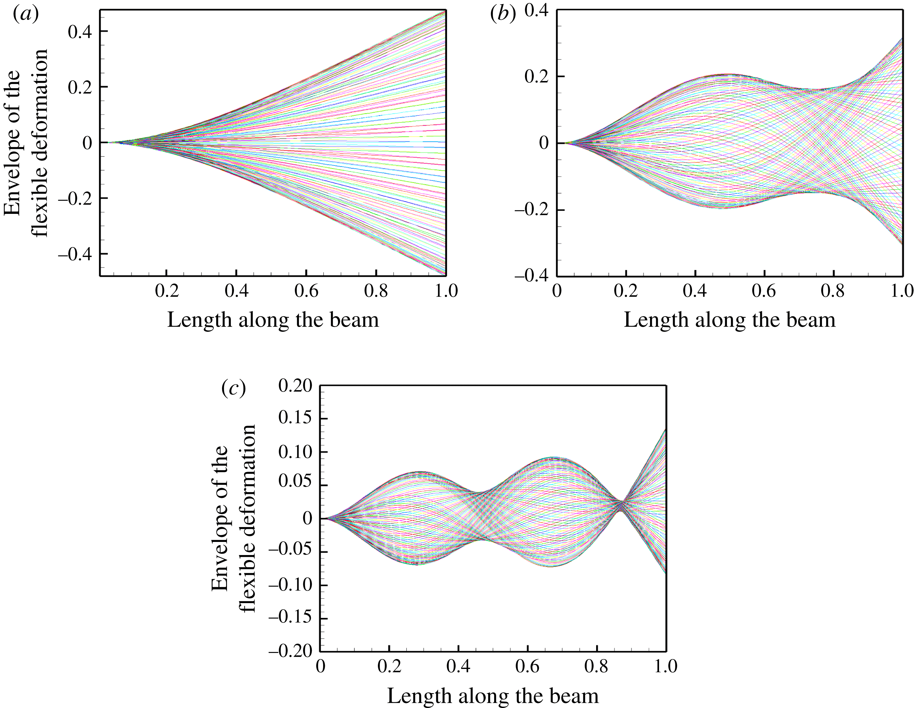
and covers the first three in-vacuum natural mode frequencies of a cantilevered Bernoulli–Euler beam. The variation of the coefficient of thrust with excitation frequency is shown in figure 5(a). The thrust maxima occur at three frequencies for the frequency range of excitation considered. These frequencies are listed in column four of table 1. The deflection patterns of the foil at these three thrust maxima frequencies, for
 ${\it\mu}=0.33$
, are shown in figure 7. Note that the deflection pattern at
 $\bar{{\it\Omega}}=2$
is predominantly the first natural mode, while the deflection pattern at
 $\bar{{\it\Omega}}=16$
is a combination of first and second natural modes, and the one at
 $\bar{{\it\Omega}}=45$
is a combination of first and third natural modes of oscillation.
Natural frequencies
 $\bar{{\it\omega}}_{i}$
and resonance frequencies
 $\bar{{\it\Omega}}_{i}$
.
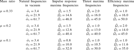
For a mass ratio
 ${\it\mu}=0.33$
, the three thrust maxima occur at frequencies lower than the natural frequencies in vacuum of a cantilevered Bernoulli–Euler beam in flexure. These natural frequencies are listed in table 1, column two, and obviously they are independent of variation in mass ratio. There
 $\bar{{\it\omega}}_{i}={\it\omega}_{i}/{\it\omega}_{c}$
where
 ${\it\omega}_{i}$
are the natural frequencies.
Now, if one were to compare the thrust maxima with the foil trailing-edge velocity at different harmonic excitation frequencies, as shown in figure 5(c), one notices that the corresponding maxima for both the responses occur at the same frequencies with the exception of the thrust peak at
 $\bar{{\it\Omega}}_{1}=2.0$
. Excluding
 $\bar{{\it\Omega}}_{1}=2.0$
, the scaled trailing-edge velocity maxima correlates well with the thrust maxima, as indeed it should since thrust is largely due to the net momentum imparted to the fluid. These observations seem to correlate well with the observations made by Quinn et al. (Reference Quinn, Lauder and Smits2014, figures 4 and 15) in the context of a heaving flexible panel, Marais et al. (Reference Marais, Thiria, Wesfreid and Godoy-Diana2012, pp. 663–664) in the case of a pitching flexible foil and Michelin & Smith (Reference Michelin and Smith2009, figure 7) in numerical studies of a flexible foil using a potential flow model, such that the thrust maxima occur when the foil trailing-edge displacement amplitude is high.
Thrust by flapping is due to the momentum imparted to the fluid by the flapping propulsor, and in that context, high flapping velocity at the trailing edge implies high momentum imparted to the fluid and therefore high thrust. In contrast, at low frequencies, the foil trailing edge velocity magnitude is relatively small and the thrust generating mechanism is driven by the leading-edge vortex – as we will discuss in more detail later in this study. To put it another way, thrust in the low-frequency range is circulatory in origin, whereas at moderate and high frequencies it is non-circulatory.
Returning to figure 5(c), note that the maximum trailing-edge velocity occurs at
 $\bar{{\it\Omega}}=16$
when
 ${\it\mu}=0.33$
. The thrust coefficient at this frequency and mass ratio is also greater than at all excitation frequencies that we simulated. Now, as the mass ratio increases from
 ${\it\mu}=0.1$
to
 ${\it\mu}=0.33$
, the maximum thrust coefficient observed is also higher – indicating once again that the momentum transferred to the fluid is greater due to heavier solid mass.
A similar pattern is observed, figure 5(d), if we determine the frequency variation of the flexible foil’s angle of incidence at its trailing edge. Here, the trailing-edge angle of incidence was calculated after ignoring the rigid-body velocity represented by
 $\text{d}\bar{h}_{b}/\text{d}{\it\tau}$
. Note that these angles are quite high, especially in the mid and high-frequency regions of flapping, and in fact would violate the assumptions that form the basis of the Bernoulli–Euler model. However, although quantitatively there will be a change, especially in the location and magnitude of the peaks, qualitatively these curves should show more or less the same trend.
Further, note that low excitation frequencies are associated with low trailing-edge velocity, low trailing-edge angle of incidence but high efficiency. The thrust coefficient does show a peak in the low frequency range but it is relatively small when compared with the local maxima observed at higher frequencies. The thrust maxima at
 $\bar{{\it\Omega}}_{1}=2.0$
has to do with formation of a leading-edge vortex, as discussed later and seen in figure 9. The propulsive efficiency is high in the low-frequency range of
 $1\leqslant \bar{{\it\Omega}}\leqslant 8$
and decreases for frequencies beyond, though efficiency maxima occur close to the frequencies of thrust maxima. High efficiencies at low frequencies is a combination of moderate thrust and low input power. The low input power here is a consequence of low frequency of oscillation; at moderate and high frequencies, it is due to the phase relation between inertial pressure forces and foil flapping frequency – we discuss this in more detail in § 4, where we examine the relation between vorticity and elastodynamics. Quinn et al. (Reference Quinn, Lauder and Smits2014, p. 263) also state that propulsive efficiency is highest at low flow speeds and high flexibilities, which agrees with the results and observations we have made here.
We also computed the thrust values of a rigid airfoil oscillating at the frequencies at which the flexible foil with mass ratio
 ${\it\mu}=0.33$
has a thrust maxima – that is, at
 $\bar{{\it\Omega}}=2,16,45$
. The thrust coefficient for the rigid airfoil at these three frequencies, respectively, have values
 $C_{t}=0.1141,0.0459,-0.2805$
. The negative sign indicates drag. The corresponding propulsive efficiency values for the first two frequencies are
 ${\it\eta}=0.006,0.02$
, respectively. This is shown in figure 5(a,b) and is denoted by solid triangles. Comparing the values of the thrust coefficient of the flexible foil with those of a rigid airfoil, the thrust and efficiency levels of the flexible foil are significantly greater, ranging from many times to a few orders of magnitude more. A similar observation, that thrust levels are three times that of a rigid foil oscillating in pitch, was made by Marais et al. (Reference Marais, Thiria, Wesfreid and Godoy-Diana2012, pp. 663–664) in the context of a pitching flexible tear-drop shaped airfoil.
The thrust coefficient, foil trailing edge velocity and foil trailing-edge angle of incidence all show a definite pattern when the mass ratios are lowered. For a given fluid, we observe that denser or heavier foils generate more thrust, have higher foil trailing-edge velocity and their angle of incidence is larger. The propulsive efficiency though is not so consistent, either across mass ratios or frequency range. Heavier foils are less efficient in the frequency range
 $35<\bar{{\it\Omega}}\leqslant 60$
. But in the range
 $1\leqslant \bar{{\it\Omega}}\leqslant 8$
and
 $8<\bar{{\it\Omega}}\leqslant 30$
there is no clear trend. In fact,
 ${\it\mu}=0.2$
generates thrust most efficiently in these two frequency ranges. We will study the cause of this in more detail later. However, it is of some interest to note that Pederzani & Haj-Hariri (Reference Pederzani and Haj-Hariri2006, figure 9, p. 2777) have shown that, for a rigid airfoil with a flexible trailing edge, a heavier airfoil is more efficient in generating thrust.
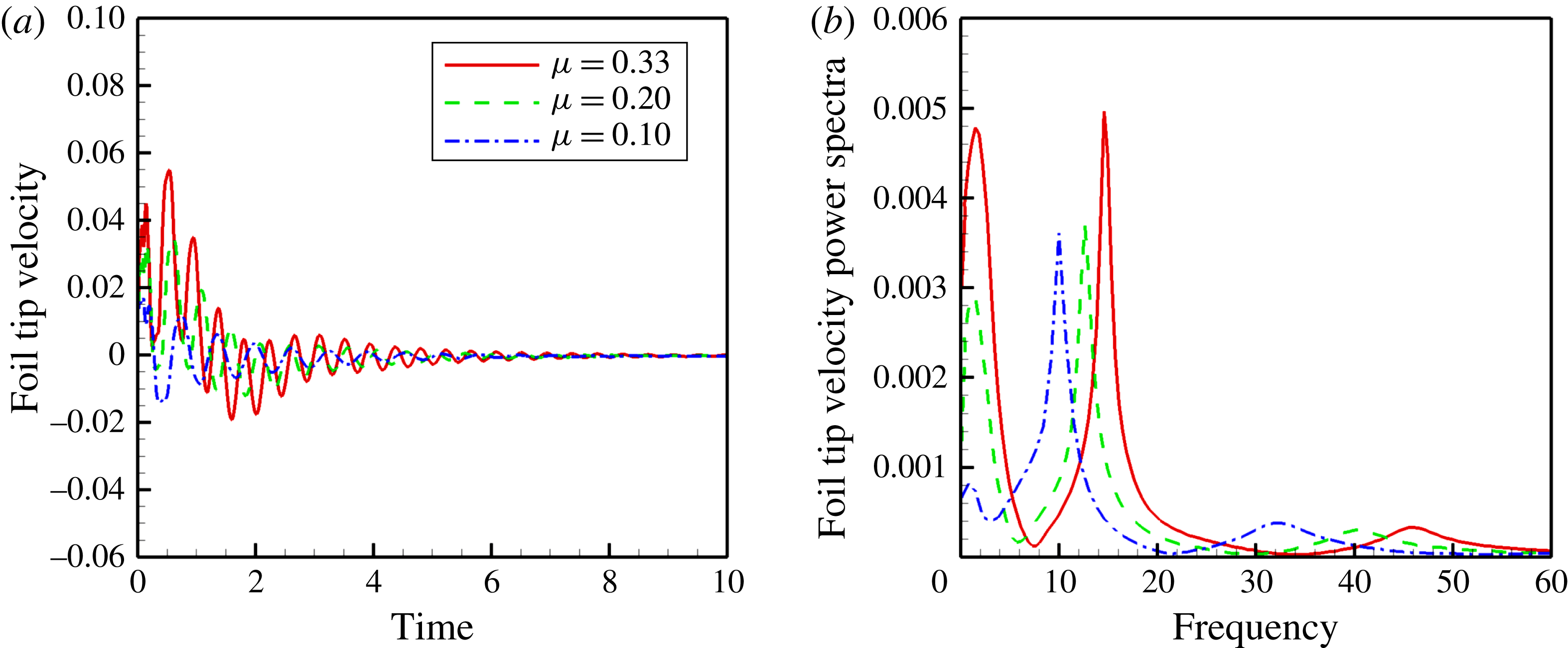
We also subjected the cantilevered foil in the viscous fluid flow to an impulse at its trailing edge and measured the flapping velocity there. The spectrum of this foil trailing-edge velocity response, together with the time signature, is shown in figure 6. The thrust maxima and foil trailing-edge velocity impulse response maxima do not coincide but are very close to each other – compare the second and third columns in table 1. That the natural frequencies, the trailing-edge impulse response flapping velocity resonance frequencies and the thrust maxima frequencies do not coincide but are close to each other is not surprising, and is as expected due to the fluid induced damping.
Foil trailing-edge velocity impulse response in the time and frequency domain for different mass ratio: (a) impulse response, (b) frequency response.
4. Vorticity and elastodynamics
Given the thrust and propulsive efficiency variation with frequency and mass ratio, we immediately notice three regions of response behaviour grouped in terms of frequency range. These regions occur around the frequencies where thrust and propulsive efficiency maxima occur. This narrative focuses its attention almost exclusively on the system with mass ratio
 ${\it\mu}=0.33$
. The first region falls within the frequency range
 $1\leqslant \bar{{\it\Omega}}\leqslant 8$
that we will call the mode-I region. The deflection pattern of the foil with mass ratio
 ${\it\mu}=0.33$
, immersed in a fluid at Reynolds number
 $Re=1000$
and oscillating with a frequency
 $\bar{{\it\Omega}}=2$
is shown in figure 7(a). This deflection pattern is similar to that of the first in-vacuum mode of a cantilevered beam. The second region, or mode-II region, falls within
 $10<\bar{{\it\Omega}}\leqslant 30$
. The deflection pattern of the foil in the fluid flow but at a frequency of
 $\bar{{\it\Omega}}=16$
is shown in figure 7(b). The deflection shape is close to that of the second mode shape of a cantilevered beam vibrating in vacuum with the exception that there is no node or point of zero displacement between the two ends of the foil. And the third, mode-III region,
 $35<\bar{{\it\Omega}}\leqslant 60$
corresponds to an excitation frequency of
 $\bar{{\it\Omega}}=45.0$
, and the deflection pattern – figure 7(c) – is close in shape to the third in-vacuum mode, but once again with only one node, in contrast to the natural mode that has two nodes. Note that similar deflections of the foil were observed in the water tunnel experiments of Quinn et al. (Reference Quinn, Lauder and Smits2014, figure 6).
Deflection patterns at thrust maxima of the flexible foil oscillating in a fluid flow;
 ${\it\mu}=0.33$
: (a)
 $\bar{{\it\Omega}}=2.0$
; (b)
 $\bar{{\it\Omega}}=16.0$
; (c)
 $\bar{{\it\Omega}}=45.0$
.
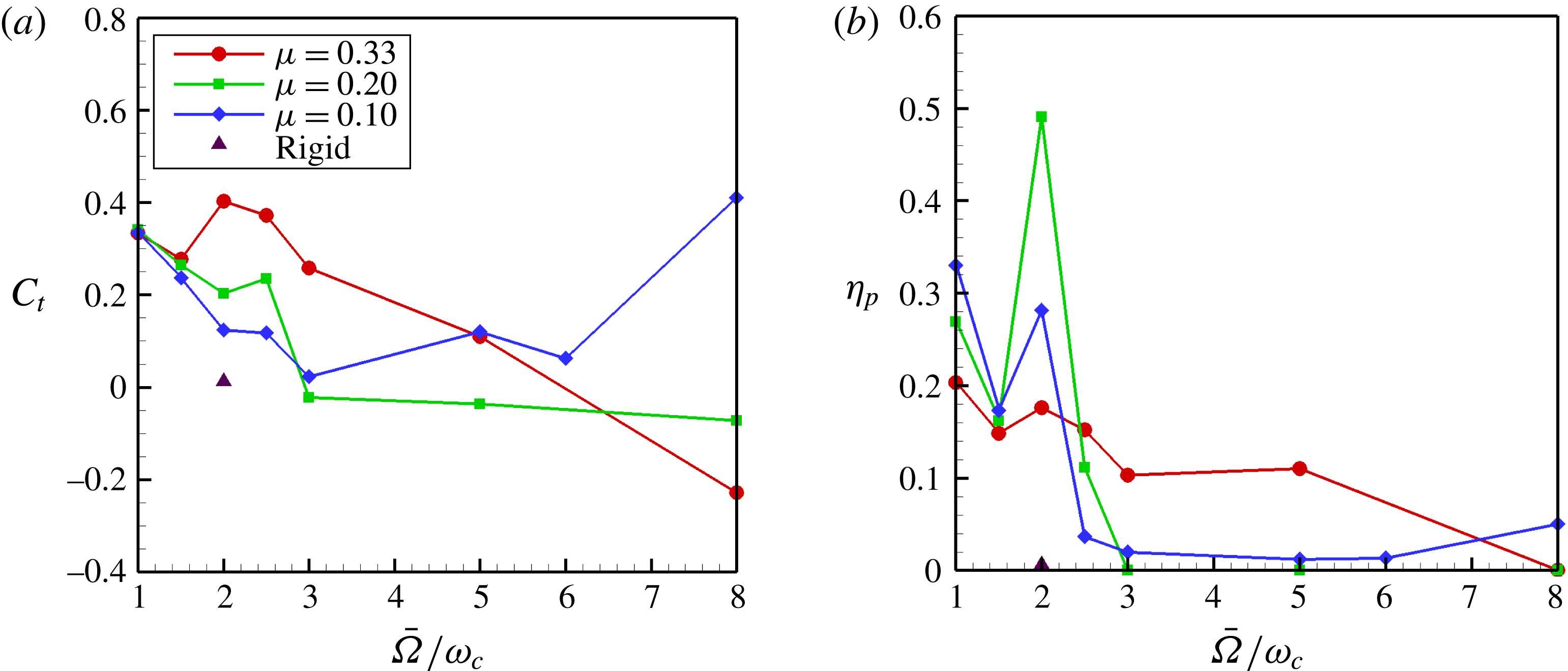
Propulsive performance for
 $1\leqslant \bar{{\it\Omega}}\leqslant 8$
: (a) thrust coefficient,
 $C_{t}$
, (b) propulsive efficiency,
 ${\it\eta}_{p}$
.
We now examine the response of the flexible propulsor in terms of its vorticity dynamics and elastodynamics in these three subsets of the excitation frequency range.
4.1. Mode-I
In figure 8 the thrust coefficient and propulsive efficiency are shown in the mode-I region in a frequency bandwidth of
 $1\leqslant \bar{{\it\Omega}}\leqslant 8$
. There are four events discernible in figure 8 that we will interrogate closely in this study. The first is the high thrust coefficient case at
 ${\it\mu}=0.33$
and a frequency of
 $\bar{{\it\Omega}}=2$
. This is followed by the low thrust event at
 ${\it\mu}=0.33$
and a frequency of
 $\bar{{\it\Omega}}=1$
. Thirdly, we discuss the high efficiency event at
 ${\it\mu}=0.2$
and a frequency of
 $\bar{{\it\Omega}}=2$
. Finally, there is drag at
 ${\it\mu}=0.33$
,
 $\bar{{\it\Omega}}=8$
. The focus in studying these four events is to explore the inter-relationship of fluid dynamics and elastodynamics in generating high thrust and efficiency, low thrust and drag.
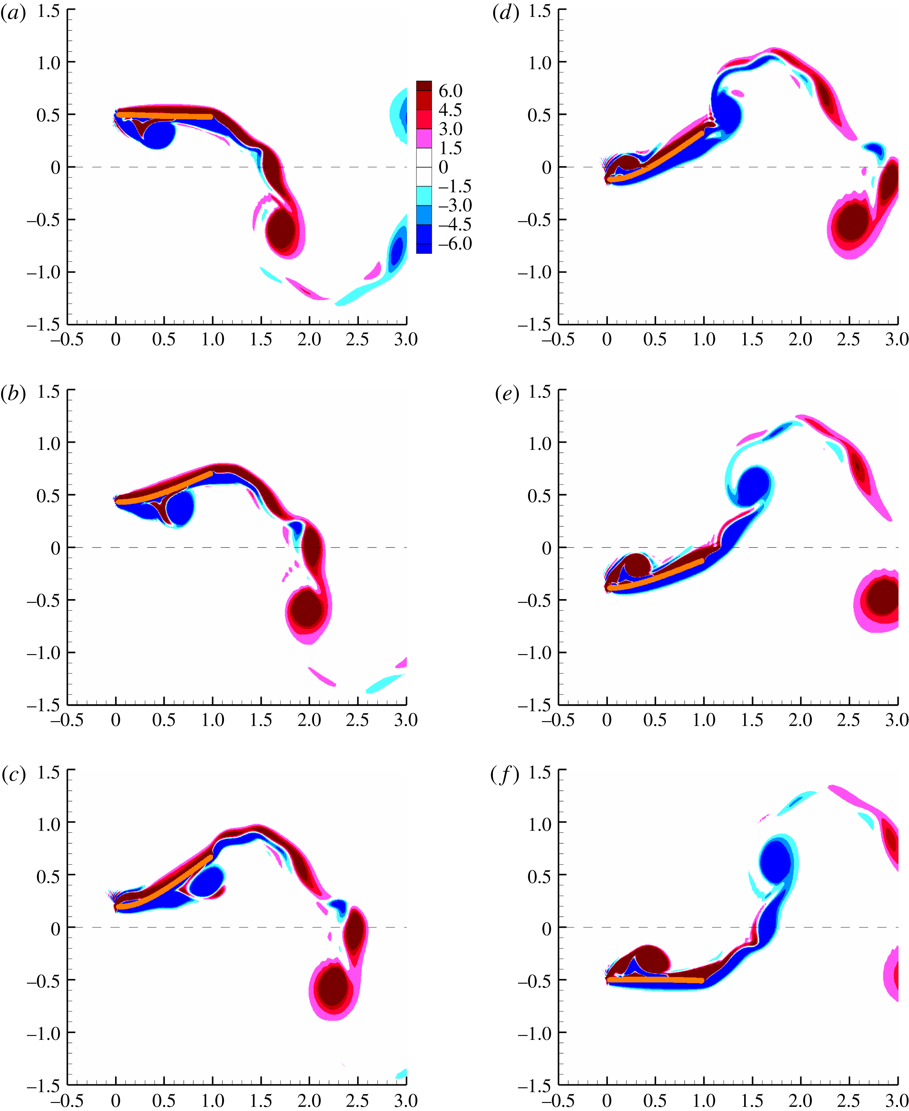
Wake vorticity contours at
 $\bar{{\it\Omega}}=2.0$
and
 ${\it\mu}=0.33$
. (a)
 $\bar{{\it\Omega}}{\it\tau}={\rm\pi}/2$
; (b)
 $\bar{{\it\Omega}}{\it\tau}={\rm\pi}/2+{\rm\pi}/5$
; (c)
 $\bar{{\it\Omega}}{\it\tau}={\rm\pi}/2+2{\rm\pi}/5$
; (d)
 $\bar{{\it\Omega}}{\it\tau}={\rm\pi}/2+3{\rm\pi}/5$
; (e)
 $\bar{{\it\Omega}}{\it\tau}={\rm\pi}/2+4{\rm\pi}/5$
; (f)
 $\bar{{\it\Omega}}{\it\tau}=3{\rm\pi}/2$
.
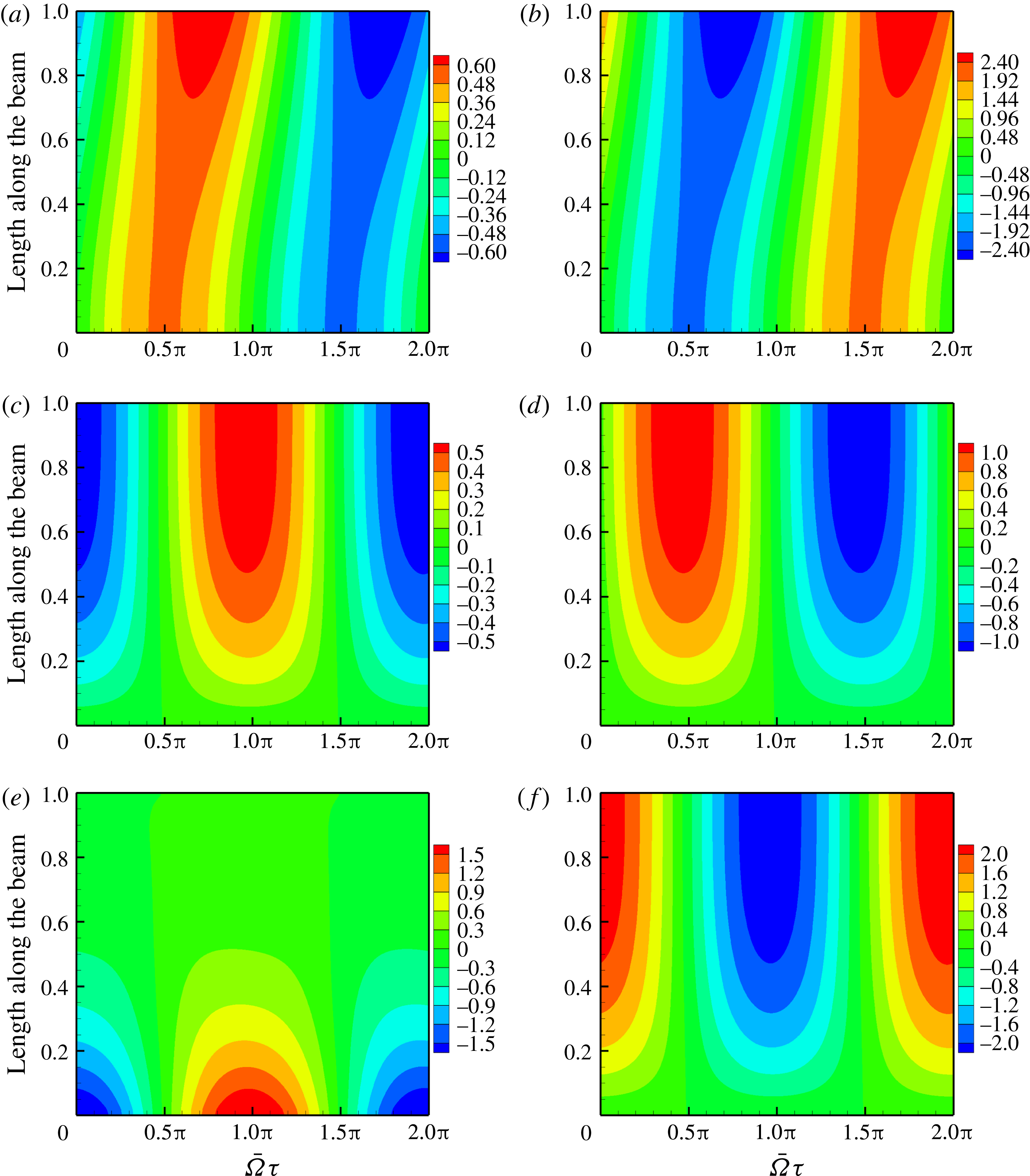
Contours of elastodynamics for
 $\bar{{\it\Omega}}=2.0$
and
 ${\it\mu}=0.33$
: (a) foil displacement, (b) foil acceleration, (c) foil slope, (d) foil angular velocity, (e) foil curvature, (f) foil angular acceleration.
4.1.1. High thrust –
 ${\it\mu}=0.33$
,
$\bar{{\it\Omega}}=2$


Figure 9 shows six snapshots of the wake contours at
 $\bar{{\it\Omega}}=2.0$
for one half-period of the oscillation cycle. A supplementary movie depicting the evolution and transport of vorticity as the flexible foil oscillates corresponding to the frequency
 $\bar{{\it\Omega}}=2$
is available at http://dx.doi.org/10.1017/jfm.2015.659. The foil motion is shown during a down stroke starting when the leading edge of the foil is at the top. At the start of the down stroke – figure 9(a) – the flexible foil is almost aligned with the free stream with a leading-edge vortex already formed on the bottom surface of the foil at the end of the previous up stroke. Note that the leading-edge vortex extends from leading edge to mid-chord and comprises of a primary vortex placed aft, and a secondary vortex placed fore, both of the same sign. In between lies a sliver of vorticity of opposite sign. As the clamped leading edge of the foil progresses along its down stroke, the foil curvature and foil slope become gradually positive. The positive slope – figure 10(c) – and curvature – figure 10(e) – create a favourable pressure gradient that accelerates the flow and prevents flow separation on the bottom surface of the flexible foil. Of course, as the primary leading-edge vortex moves beyond the mid-chord, figure 9(b–d), the flow de-accelerates and the primary leading-edge vortex separates near the trailing edge. The secondary leading-edge vortex that is formed on the lower surface following the primary leading-edge vortex, and having the same sign, is stretched along the lower surface as it is transported, and ultimately shed, at the trailing edge, together with shreds of vorticity of the opposite sign from the upper and lower surfaces of the foil – figure 9(a–f). The remaining half-cycle shows a mirror image vorticity and foil deflection pattern; the wake as well as the foil deflection figure 7(a) are symmetric and no asymmetry is noticed.
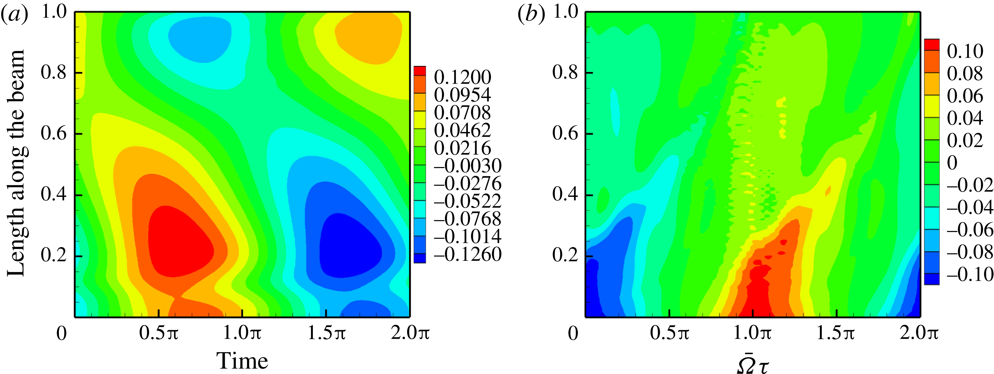
Figure 10 shows the contours of kinematics of the elastic response of the foil for
 $\bar{{\it\Omega}}=2.0$
. The abscissa corresponds to one time period of excitation with
 $\bar{{\it\Omega}}{\it\tau}=0$
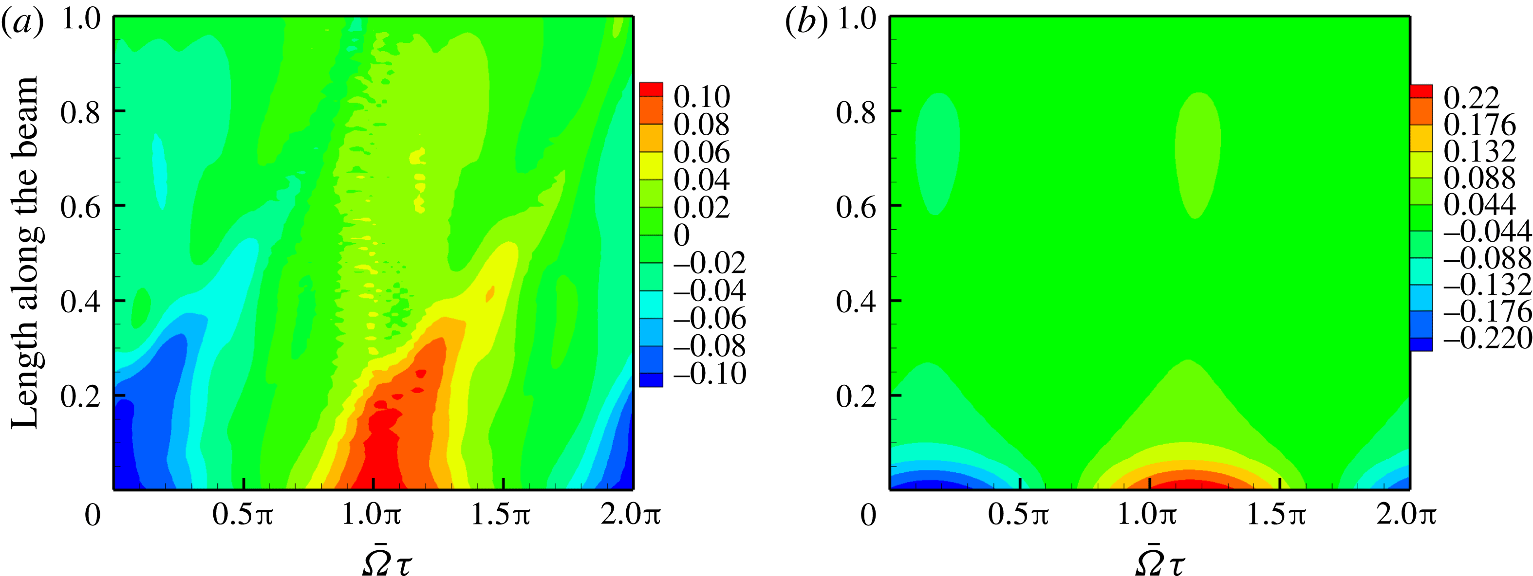
corresponding to when the leading edge or the clamped end of the foil is at the mean position; the ordinate of the plots denotes the length of the foil. In particular, note the foil slope and curvature – figure 10(c,e) – and the differential pressure figure 11(a). The pressure on the foil is generated in regions where the curvature and slope are high. This is the region where the primary leading-edge vortex is formed and transported before losing its strength further aft of the mid-chord, as can be seen in the snapshots in figure 9. Together, the curvature and slope, create a favourable pressure gradient relative to the free stream that sustains the leading-edge vortex without allowing it to separate. The leading-edge vortex is created due to the high effective angle of incidence induced by the foil slope and flapping velocity. The pressure contour figure 11(a) is tilted to the right, indicative of a forward moving pressure disturbance due to the movement of the leading-edge vortex towards the trailing edge. In the same pressure contour plot, figure 11(a), there is a region between
 $0.6<\bar{x}<0.8$
along the length of the foil where there are small narrow islands of high differential pressure. These are caused by the transverse and angular accelerations of the foil, as well as its angular velocity – figure 10(b,d,f). Thus this high pressure region is predominantly non-circulatory in origin.
Viscous and potential fluid flow pressure contours;
 $\bar{{\it\Omega}}=2.0$
and
 ${\it\mu}=0.33$
: (a) differential pressure – viscous, (b) differential pressure – potential.
The choice of foil motion parameters chosen in figure 10 has to do with the unsteady lift experienced by an oscillating airfoil in pitch and heave in a two-dimensional potential flow. Although we simulated a viscous fluid, we have taken results from potential flow theory in order to gain an idea of the functional dependence of unsteady pressure on foil motion parameters. Closed-form expressions that clearly state the functional dependence of the unsteady pressure on the foil motion parameters can be derived for unsteady, incompressible potential flow. The unsteady differential pressure in potential flow theory is a function of the angular velocity, angular acceleration and transverse acceleration of the foil (Fung Reference Fung1955, p. 209). Symbolically
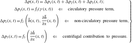 $$\begin{eqnarray}\left.\begin{array}{@{}c@{}}{\rm\Delta}p(x,t)={\rm\Delta}p_{1}(x,t)+{\rm\Delta}p_{2}(x,t)+{\rm\Delta}p_{3}(x,t);\\ {\rm\Delta}p_{1}(x,t)=f_{1}({\it\gamma}(x,t))\quad \Leftarrow \quad \text{circulatory pressure term},\\ \displaystyle {\rm\Delta}p_{2}(x,t)=f_{2}\left(\ddot{h}(x,t),\frac{\partial \ddot{h}}{\partial x}(x,t)\right)\quad \Leftarrow \quad \text{non-circulatory pressure term},\\ \displaystyle {\rm\Delta}p_{3}(x,t)=f_{3}\left(\frac{\partial {\dot{h}}}{\partial x}(x,t)\right)\quad \Leftarrow \quad \text{centrifugal contribution to pressure}.\end{array}\right\}\end{eqnarray}$$
The curvature of the foil is included as one of the motion parameters that influence the pressure and vorticity over the foil since it is indicative of change in slope and affects the pressure gradient. Once again, we would like to reiterate that this break down of pressure forces on the oscillating foil is based on unsteady potential flow theory; it only gives us an approximate dependence of vorticity and pressure on motion variables when viscous effects are present.
We compared the differential pressure for the viscous fluid – figure 11(a) – with that for a potential flow – figure 11(b). The leading-edge region shows a qualitatively different pressure loading primarily due to the transport of the leading-edge vortex over it. The rightward tilt of the pressure contour from the leading edge is absent for the potential flow simulation as now there is no formation and transport of the leading-edge vortex.
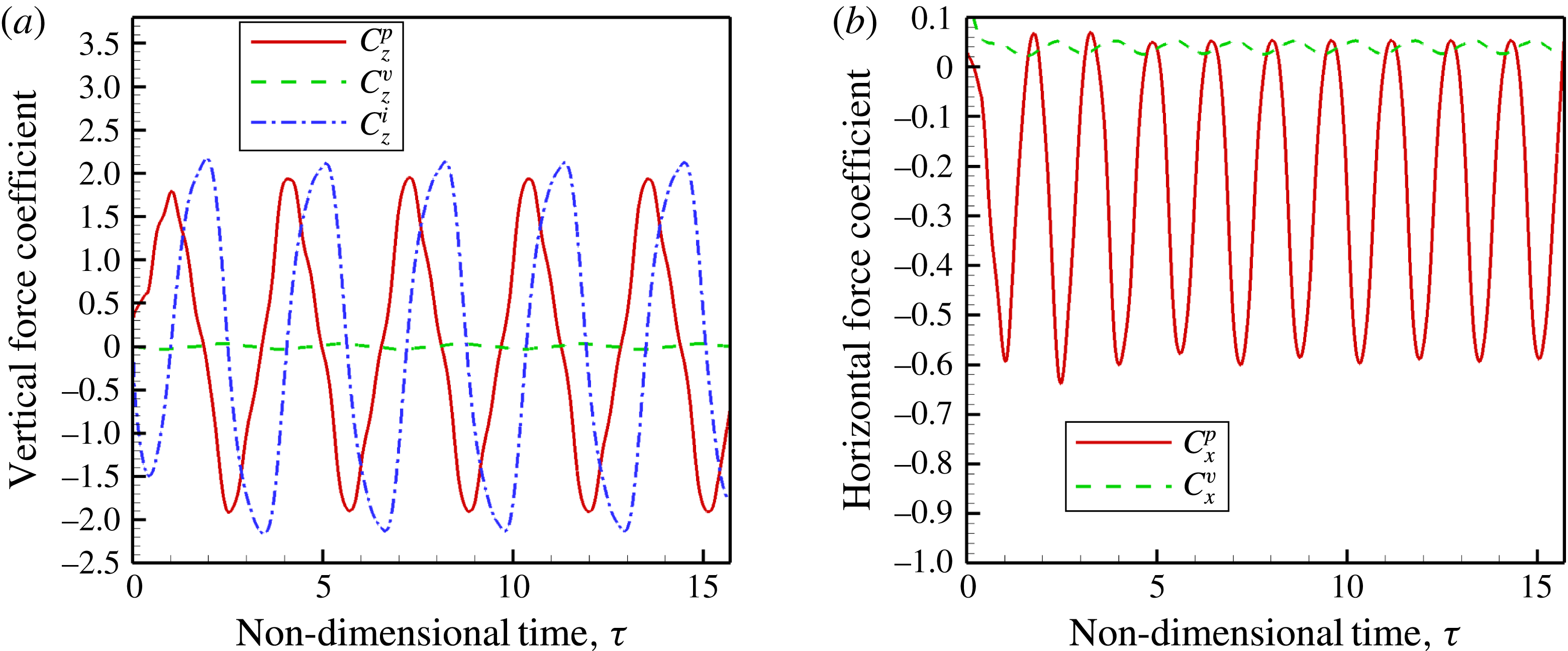
Figure 12 shows the coefficient of forces perpendicular and parallel to free stream. In figure 12(a) the viscous force coefficient
 $$\begin{eqnarray}C_{z}^{v}=\frac{1}{1/2{\it\rho}U_{\infty }^{2}}\int _{0}^{L}{\it\mu}\left(\frac{\partial u_{\hat{t}}}{\partial \hat{n}}+\frac{\partial u_{\hat{n}}}{\partial \hat{t}}\right){\rm\Delta}x\hat{\boldsymbol{t}}\boldsymbol{\cdot }\hat{\boldsymbol{k}}\,\text{d}x,\end{eqnarray}$$
in the vertical direction is very small and effectively contributes zero lift force over one period of the oscillation. On the other hand, the lift due to the pressure force, also shown in figure 12(a), is defined as
 $$\begin{eqnarray}C_{z}^{p}=\frac{1}{1/2{\it\rho}U_{\infty }^{2}}\int _{0}^{L}{\rm\Delta}p(x,t)\hat{\boldsymbol{n}}\boldsymbol{\cdot }\hat{\boldsymbol{k}},\end{eqnarray}$$
and is significant even though this too contributes no net vertical force over one cycle of oscillation. Note that the lift force due to pressure is not harmonic, even though the excitation is harmonic. This is a consequence of the nonlinear nature of the system. We have also shown the inertia force coefficient in figure 12(a)
 $$\begin{eqnarray}C_{z}^{i}=\frac{1}{1/2{\it\rho}U_{\infty }^{2}}\int _{0}^{L}-m(\ddot{h}(x,t)+\ddot{h}_{b}(t))\,\text{d}x.\end{eqnarray}$$
In fact, its magnitude is greater than that of the component of the pressure force in the vertical direction and it is out-of-phase with the pressure force.
Forces perpendicular and parallel to free stream for
 $\bar{{\it\Omega}}=2.0$
and
 ${\it\mu}=0.33$
: (a) forces in the vertical direction, (b) forces in the free-stream direction.
Phase difference between force and slope: (a)
 ${\it\phi}=0$
; (b)
 ${\it\phi}={\rm\pi}/2$
; (c)
 ${\it\phi}={\rm\pi}$
.
Forces in the horizontal or free-stream direction are components due to viscous and pressure forces and the viscosity induced drag force is almost an order of magnitude lower than the pressure induced thrust force – figure 12(b).
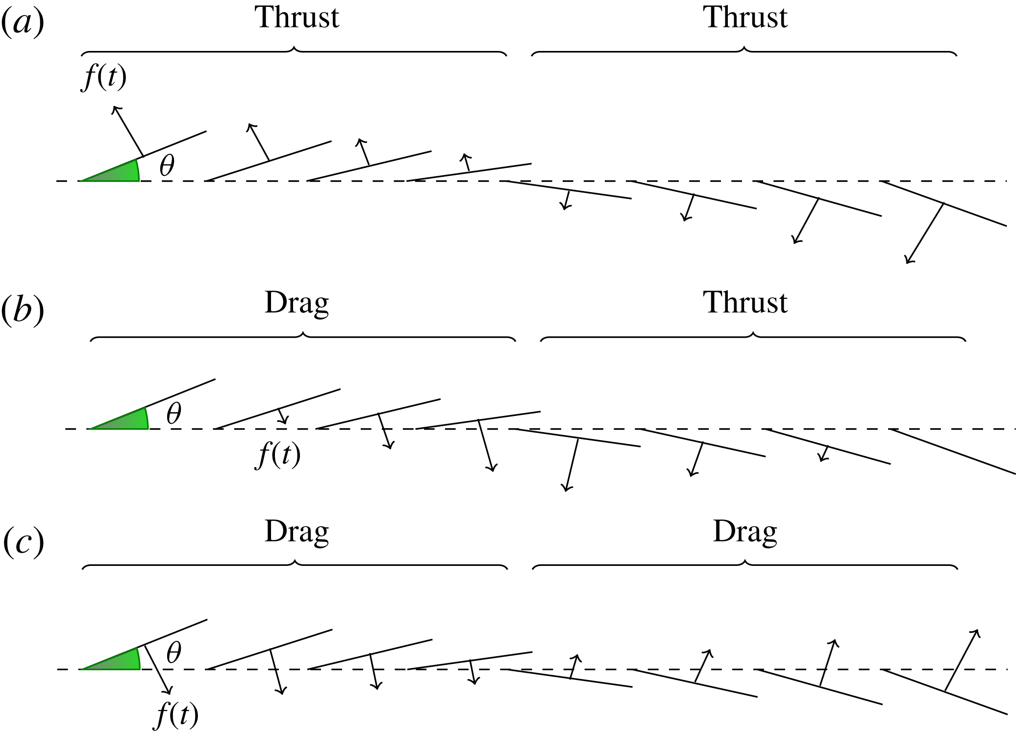
As shown in figure 12, viscous forces contribute very little to forces on the foil in both vertical and horizontal directions. In the horizontal direction, it is primarily the pressure force component that is significant. The component of the pressure force in the horizontal direction that eventually contributes to drag is dependent on the phase relation between the pressure force and slope of the foil at any given point on the flexible foil. We have illustrated this in figure 13. When the phase difference between the pressure force and slope at any given point on the foil is zero, that is
 ${\it\phi}=0$
, then the pressure force and slope vary synchronously and they give rise to a thrust force throughout the cycle. When the phase difference
 ${\it\phi}={\rm\pi}/2$
or
 $3{\rm\pi}/2$
at a given point on the foil, then for one half of the cycle, the pressure force contributes to thrust and for the other half, it contributes to drag; the net thrust is zero. Finally, when
 ${\it\phi}={\rm\pi}$
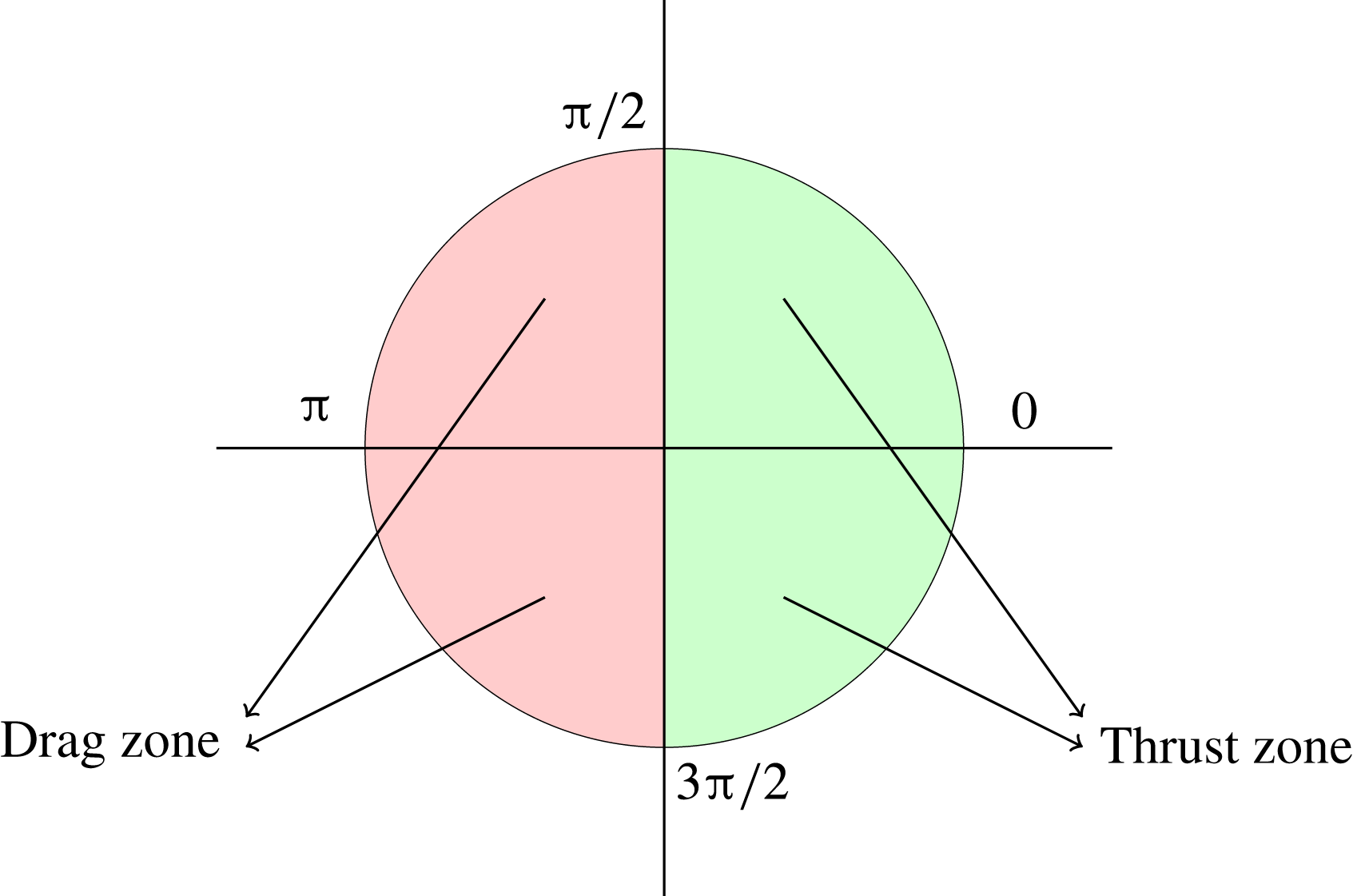
, then throughout the cycle the pressure force only contributes to drag at a given point on the foil. When the phase difference lies in between these values then they could give rise to either a net thrust or drag in one cycle at a given point on the foil. These instances can be best illustrated and summarised in the pie chart figure 14. A phase difference between
 $[0,{\rm\pi}/2)$
and
 $(3{\rm\pi}/2,2{\rm\pi}]$
will generate thrust. However when the phase difference lies between
 $({\rm\pi}/2,{\rm\pi}]$
and
 $[{\rm\pi},3{\rm\pi}/2)$
the pressure will contribute only to drag.
Thrust, drag and pressure–slope phase relation.
Phase difference
 ${\it\phi}$
between foil kinematics and forces;
 $\bar{{\it\Omega}}=2.0$
and
 ${\it\mu}=0.33$
: (a) pressure and slope, (b) force and
 $\text{d}\bar{h}_{b}/\text{d}{\it\tau}$
.
Now, if we plot the phase difference between pressure and flexure slope of the foil, for
 ${\it\mu}=0.33$
,
 $\bar{{\it\Omega}}=2$
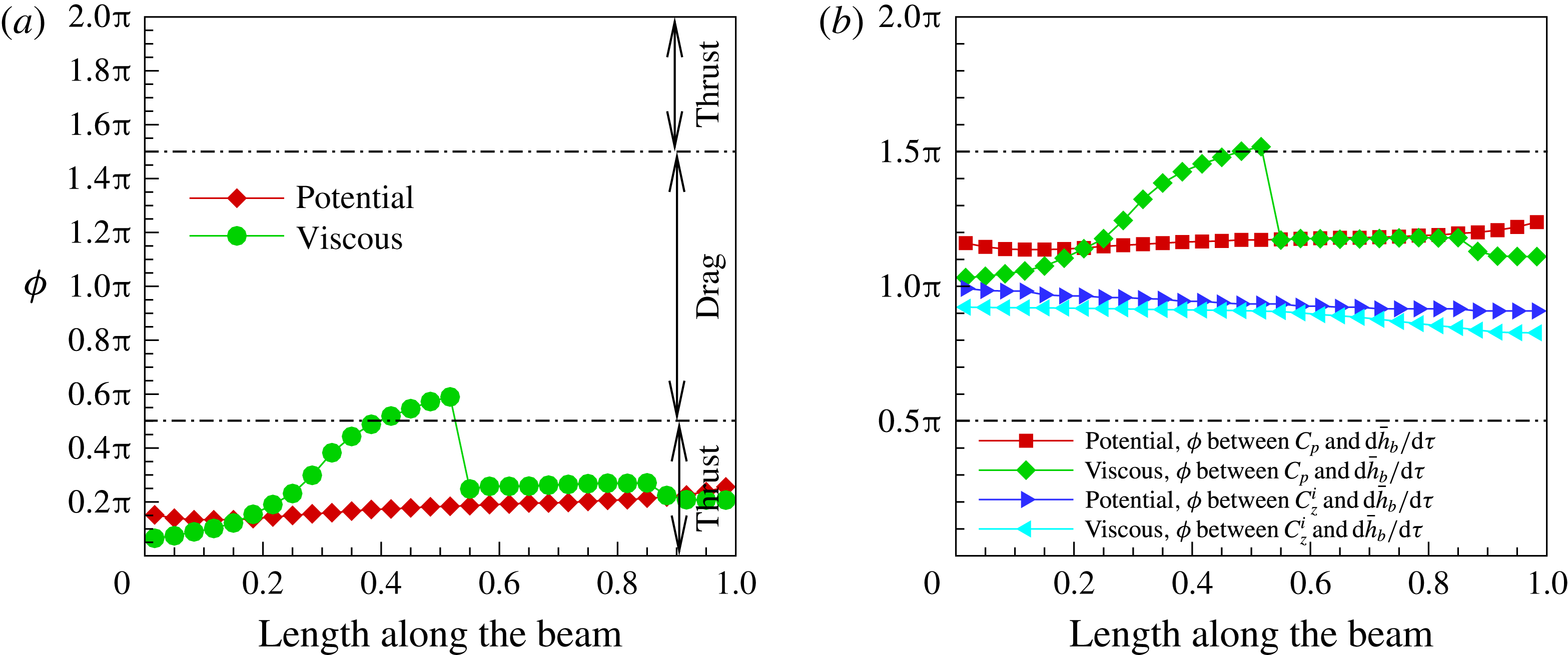
, at uniformly spaced points on the foil, then figure 15(a) is the result. For the viscous case, near the leading edge, the vortex formed causes forces which are in phase with foil slope. Note that the wake contours around the foil, figure 9, show that the leading-edge vortex extends from the leading-edge to the mid-chord with a greater concentration of vorticity there. The phase difference correspondingly increases. Beyond the mid-chord, there is a sudden jump in the phase difference, albeit still almost within
 $[0,{\rm\pi}/2]$
, because from that point onwards the non-circulatory pressure forces dominate. From the discussion on figure 10, we know that, besides differential pressure due to the leading-edge vortex, non-circulatory forces due to the acceleration and velocity of the foil also contribute to the thrust aft of the mid-chord. The phase difference for the potential flow is almost constant, and close to zero, with a slight increase along the length of the foil. Thrust computed using a potential flow model is greater than determined using the viscous flow model.
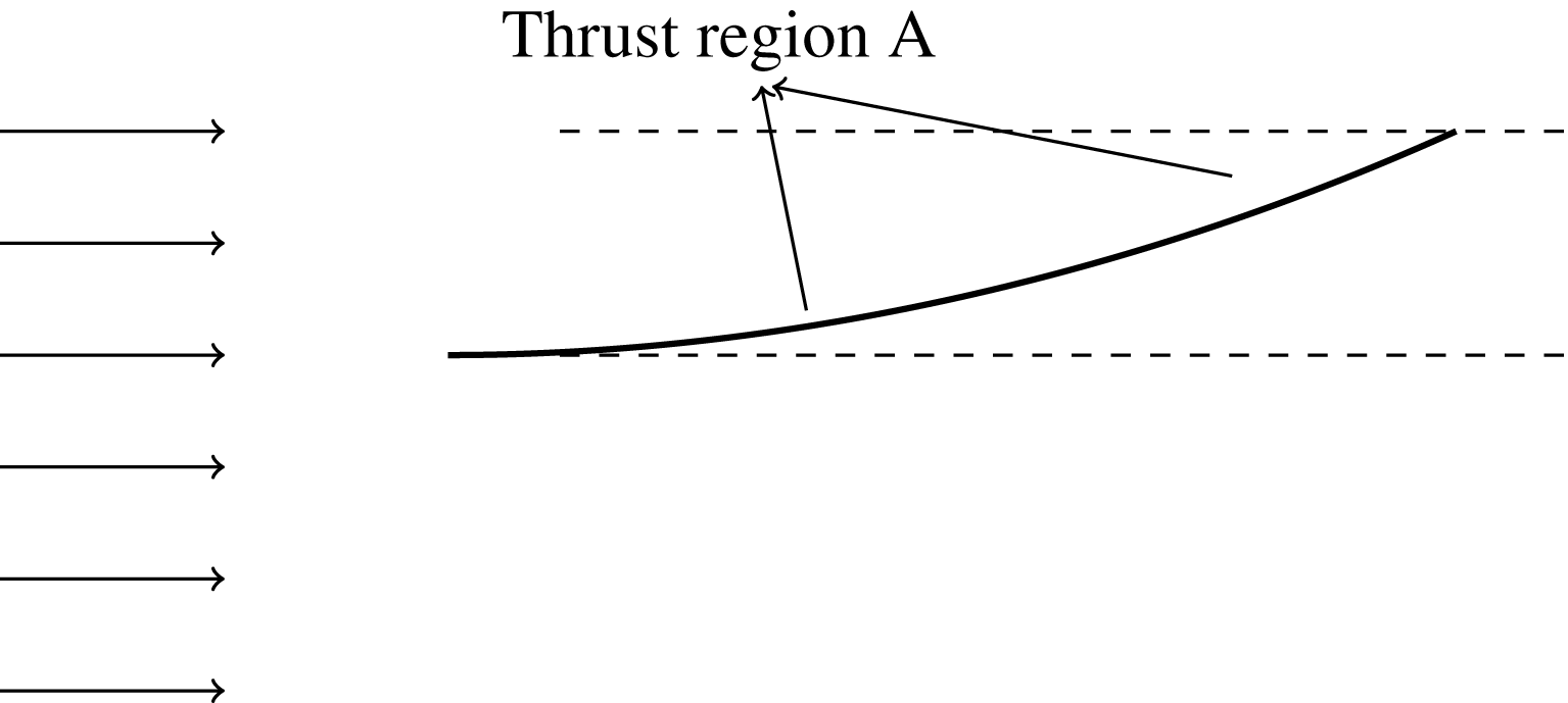
Figure 16 shows a cartoon of the deformation of the foil in the mode-I region with the thrust producing region marked. In the anterior part of the flexible foil, it is the circulatory or leading-edge vortex that induces pressure and generates thrust, while in the posterior region it is the non-circulatory pressure that contributes to thrust.
Thrust in the mode-I regime.
The power input, (3.4), comprises of two components, namely, power input due to pressure forces –
 ${\dot{h}}_{b}(t){\rm\Delta}p(x,t)\hat{\boldsymbol{n}}\boldsymbol{\cdot }\hat{\boldsymbol{k}}$
– and power input due to inertia forces –
 ${\dot{h}}_{b}(t)m(\ddot{h}(x,t)+\ddot{h}_{b}(t))$
. These two input forces are shown in figure 4. Note that a phase difference of
 $0<{\it\phi}<{\rm\pi}/2$
and
 $3{\rm\pi}/2<{\it\phi}<2{\rm\pi}$
between the transverse velocity
 ${\dot{h}}_{b}(t)$
and the pressure force or inertia force implies positive work done by the force on the system, or that energy is added to the elastic solid. A phase difference of
 ${\rm\pi}/2<{\it\phi}<3{\rm\pi}/2$
, on the other hand, denotes negative work done by the force on the system, or that energy is extracted from the deforming elastic solid. The elastic solid comprises of its flexibility and damping.
With reference to figure 15(b), the fluid pressure force does negative work throughout the length of the foil, or in other words, the elastic system loses energy to the flow. In the first half of the foil length these pressure forces are mainly caused by the leading-edge vortex. Beyond the mid-point, the pressure forces are caused primarily by the non-circulatory or inertial effects. The inertia force also does negative work on the system or subtracts energy from the elastic system throughout the length of the foil. Therefore, the power input as given by (3.4) will be positive, or in other words, an external power source will compensate for the loss of energy from the elastic system to the flow. Consequently, the propulsive efficiency at
 $\bar{{\it\Omega}}=2.0$
and
 ${\it\mu}=0.33$
, figure 8(b), is low relative to that of the other two mass ratios.
4.1.2. High efficiency –
${\it\mu}=0.2$
,
$\bar{{\it\Omega}}=2$


The maximum propulsive efficiency occurs at an excitation frequency
 $\bar{{\it\Omega}}=2.0$
for a mass ratio
 ${\it\mu}=0.2$
– figure 8(b). The propulsive efficiency defined by (3.7) is the ratio of work done by the thrust force in moving the foil with a forward speed
 $U_{\infty }$
, to the input work done by the base excitation force acting on the foil at its root. Given that the frequency of excitation is the same
 $\bar{{\it\Omega}}=2$
for high thrust
 ${\it\mu}=0.33$
and high propulsive efficiency
 ${\it\mu}=0.2$
, the input work done by inertia forces would approximately be the same for both these cases. However, the input work by the pressure force ought to be different.
The phase difference between the slope of the foil and pressure force coefficient along the length of the foil is shown for
 ${\it\mu}=0.33$
and
 ${\it\mu}=0.2$
in figure 17(a). For
 ${\it\mu}=0.33$
and high thrust, the phase difference falls within
 ${\rm\pi}/2$
almost throughout the length of the foil. The pressure on the foil therefore contributes to thrust all along the length of the foil and it is not surprising that thrust is at a maximum. However, for
 ${\it\mu}=0.2$
, the phase difference falls beyond
 ${\rm\pi}/2$
in the interval
 $x/L=0.4$
and
 $x/L=0.6$
. In this region of the foil, the pressure contributes to drag and thus the net thrust for
 ${\it\mu}=0.2$
is lower than that for
 ${\it\mu}=0.33$
.
The vorticity contours for
 ${\it\mu}=0.2$
are quite similar to that of
 ${\it\mu}=0.33$
at
 $\bar{{\it\Omega}}=2$
, figure 9. However, the slope of the foil for
 ${\it\mu}=0.2$
, when in the middle of a down stroke, is slightly greater than in the case for
 ${\it\mu}=0.33,\bar{{\it\Omega}}=2$
, as shown earlier in figure 9(e). This increase in slope is reflected in figure 17(a) for the case
 ${\it\mu}=0.2$
, where the phase difference between pressure and slope of foil crosses the
 ${\rm\pi}/2$
line and results in drag. This in turn lowers the overall thrust of the foil for
 ${\it\mu}=0.2$
.
Phase difference
 ${\it\phi}$
between forces on the foil and foil kinematics for high thrust and high-efficiency cases at
 $\bar{{\it\Omega}}=2.0$
: (a) pressure and slope, (b) force and
 $\text{d}\bar{h}_{b}/\text{d}{\it\tau}$
.
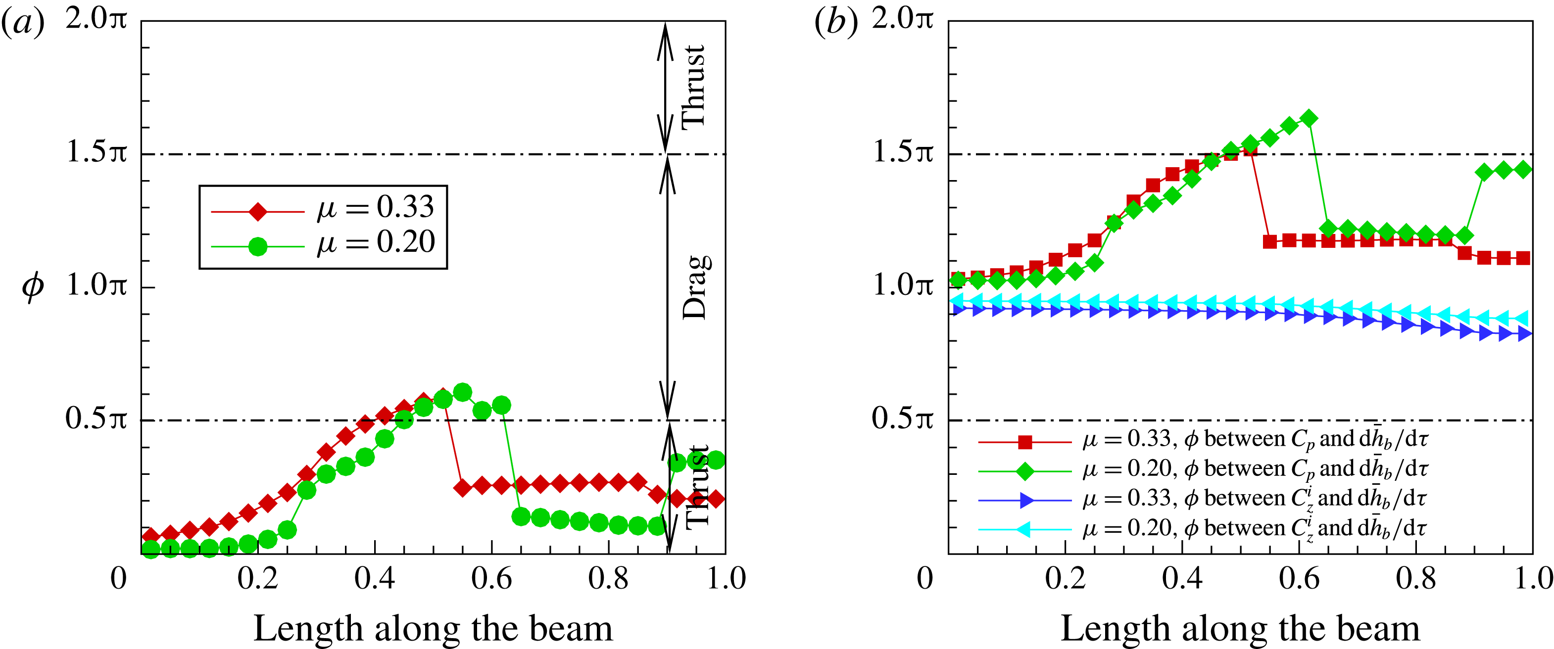
If we now focus our attention on the phase difference between the foil transverse velocity and pressure forces for
 ${\it\mu}=0.2$
in figure 17(b), one notices that between
 $0\leqslant x/L\leqslant 0.5$
, the phase difference lies in the range
 ${\rm\pi}<{\it\phi}<3{\rm\pi}/2$
; implying the pressure forces are doing negative work on the elastic foil, or the elastic foil is losing energy. This amount is compensated by the work done by the input base excitation force acting on the foil. But in the length span of
 $0.5\leqslant x/L\leqslant 0.6$
the pressure forces do positive work, or add energy to elastic foil, so that much less power or energy needs to be added by the base excitation force. Beyond
 $x/l=0.6$
pressure forces do negative work. Contrast this with the case for
 ${\it\mu}=0.33$
and notice that the pressure forces do negative work along the entire span of the foil. The inertia forces for both these mass ratios do negative work throughout the span of the foil and therefore they do not contribute to any difference in their respective input power term. Therefore, for a foil with mass ratio
 ${\it\mu}=0.2$
, since the pressure forces do positive work on the elastic foil, the input power supplied by the base excitation force is that much lower than for a foil with mass ratio
 ${\it\mu}=0.33$
, resulting in a higher propulsive efficiency.
Differential pressure for high thrust
 ${\it\mu}=0.33$
(a) and high efficiency
 ${\it\mu}=0.2$
(b); Mode-I;
 $\bar{{\it\Omega}}=2.0$
.
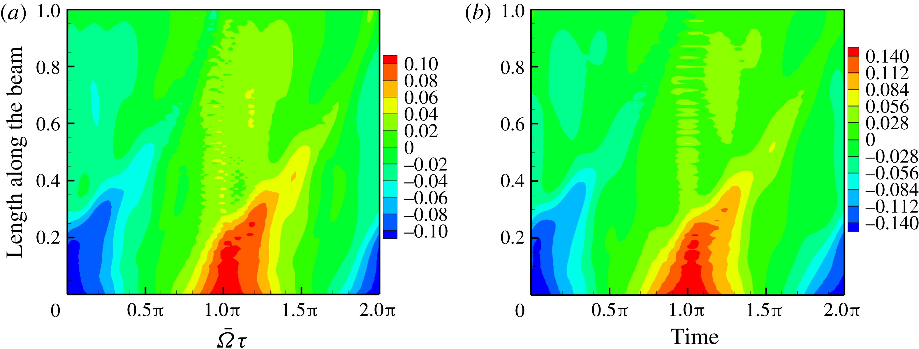
Figure 18 shows the pressure contours for
 ${\it\mu}=0.33$
and
 $0.2$
. Note that the pressure maxima is higher –
 ${\rm\Delta}p=0.14$
at
 ${\it\mu}=0.2$
compared to
 ${\rm\Delta}p=0.1$
at
 ${\it\mu}=0.33$
. But more importantly, the higher pressure differential occurs along the length at the start of the cycle in the case of
 ${\it\mu}=0.2$
. In contrast, the differential pressure seems to grow along the foil with time for
 ${\it\mu}=0.33$
, following the movement of the leading-edge vortex. Further, in figure 18(a), for
 ${\it\mu}=0.33$
, the inertia induced or non-circulatory pressure starts somewhere from
 $x/L=0.4$
and peaks around
 $x/L=0.6$
. This peak is greater than in the case for
 ${\it\mu}=0.2$
in figure 18(b). So, in the case of
 ${\it\mu}=0.33$
, higher non-circulatory pressure combined with a sympathetic phase relation of pressure with the slope of the foil contribute to higher thrust. It should be kept in mind that higher differential pressure alone is not sufficient to ensure higher thrust, but rather the phase difference between pressure and foil slope is equally important.
4.1.3. Low thrust –
${\it\mu}=0.33$
,
$\bar{{\it\Omega}}=1$


A larger high-differential-pressure region does not always lead to high thrust. As we have reiterated in the earlier examples, it is the phase difference between the pressure and foil slope that is responsible for thrust, as illustrated in figure 13. Maximum thrust is realised if the pressure and slope synchronously vary; that is, with a phase difference of
 $0$
or close to this. In order to illustrate this, we choose
 $\bar{{\it\Omega}}=1.0$
at
 ${\it\mu}=0.33$
, as here the thrust is lower than that for
 $\bar{{\it\Omega}}=2.0$
, as can be seen in figure 8(a).
Phase difference
 ${\it\phi}$
between forces on the foil and foil kinematics for
 ${\it\mu}=0.33$
at
 $\bar{{\it\Omega}}=1.0$
and
 $\bar{{\it\Omega}}=2.0$
: (a) pressure and slope, (b) force and
 $\text{d}\bar{h}_{b}/\text{d}{\it\tau}$
.
Differential pressure on the foil for
 ${\it\mu}=0.33$
at
 $\bar{{\it\Omega}}=1.0$
(a) and
 $\bar{{\it\Omega}}=2.0$
(b).

Wake vorticity contours at
 $\bar{{\it\Omega}}=1.0$
and
 ${\it\mu}=0.33$
: (a)
 $\bar{{\it\Omega}}{\it\tau}={\rm\pi}/2$
; (b)
 $\bar{{\it\Omega}}{\it\tau}={\rm\pi}/2+{\rm\pi}/5$
; (c)
 $\bar{{\it\Omega}}{\it\tau}={\rm\pi}/2+2{\rm\pi}/5$
; (d)
 $\bar{{\it\Omega}}{\it\tau}={\rm\pi}/2+3{\rm\pi}/5$
; (e)
 $\bar{{\it\Omega}}{\it\tau}={\rm\pi}/2+4{\rm\pi}/5$
; (f)
 $\bar{{\it\Omega}}{\it\tau}=3{\rm\pi}/2$
.
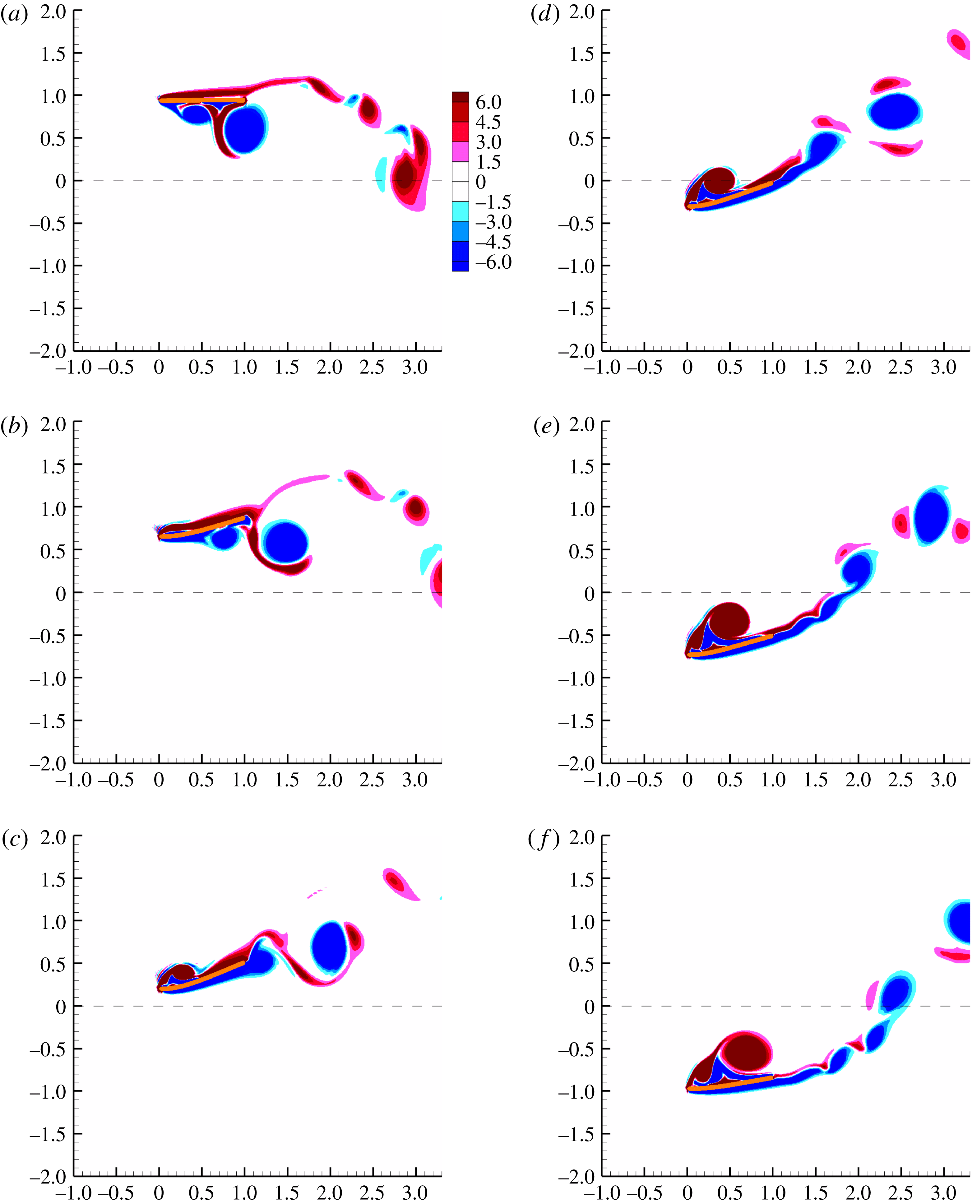
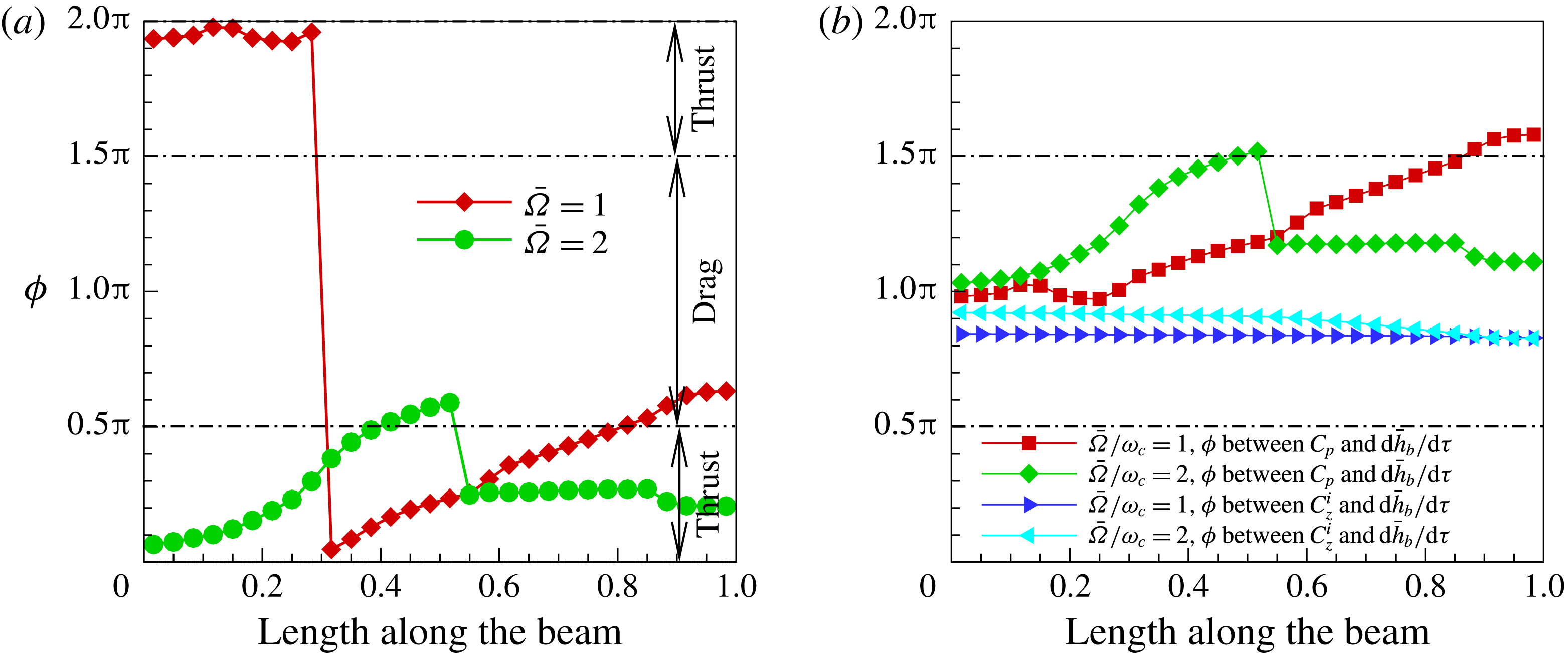
Figure 19(a) shows the phase difference between pressure and slope for two frequencies –
 $\bar{{\it\Omega}}=1.0$
and
 $\bar{{\it\Omega}}=2.0$
. The phase difference for
 $\bar{{\it\Omega}}=1.0$
crosses the
 ${\rm\pi}/2$
thrust cutoff line beyond
 $x/L=0.8$
and this contributes to lower thrust as the interval around
 $0.8\leqslant x/L\leqslant 1.0$
contributes to drag. However, note that the phase difference in the region up to
 $x/L=0.8$
is lower in value than in the case for
 $\bar{{\it\Omega}}=2.0$
, which should as such give rise to more thrust; but there are two other factors at play here: one, the significant drag caused by the trailing-edge portion, and two, as we show in figure 20(a), the differential pressure over the foil is substantially lower in magnitude than at
 $\bar{{\it\Omega}}=2.0$
. Therefore the overall thrust when oscillating at
 $\bar{{\it\Omega}}=1.0$
is much lower. In contrast, for the case when
 $\bar{{\it\Omega}}=2.0$
the drag region of the pressure-slope phase difference is almost non-existent, and therefore the overall thrust is higher.
The phase difference between the pressure and inertia forces that determines the input power, and thereby the propulsive efficiency, is shown in figure 19(b) for
 $\bar{{\it\Omega}}=1.0$
and
 $\bar{{\it\Omega}}=2.0$
. The inertia forces for both these frequencies do negative work on the elastic foil and therefore the foil loses energy to the inertia forces. However, the energy lost to inertia forces is less for
 $\bar{{\it\Omega}}=1.0$
since the frequency of excitation is lower. In the case of a pressure force at
 $\bar{{\it\Omega}}=1.0$
, the pressure force does positive work on the elastic foil in the region starting close to
 $x/l=0.85$
and terminating at the trailing edge. This then lowers the input power supplied by the external source leading to a higher propulsive efficiency relative to
 $\bar{{\it\Omega}}=2.0$
; this is indeed the case as can be seen in figure 8(b).
The vorticity contours for
 ${\it\mu}=0.33$
at a frequency of
 $\bar{{\it\Omega}}=1$
are shown in figure 21. One immediately notices that the leading-edge vorticity is much larger due to the fact that the heave amplitude
 $\bar{H}_{b}=1$
is now twice that of
 $\bar{{\it\Omega}}=2$
, as we have set
 $\bar{{\it\Omega}}\bar{H}_{b}=1$
. The leading vortex separates long before it reaches the trailing edge of the foil. Consequently, the differential pressure across the foil is lower in magnitude relative to that when
 $\bar{{\it\Omega}}=1$
. Elastodynamically, the frequency being lower, and consequently the inertia force almost four times lower than for
 $\bar{{\it\Omega}}=2$
, the foil slope is less steep. This can be noticed if one compares the vorticity contours for
 $\bar{{\it\Omega}}=2$
and
 $\bar{{\it\Omega}}=1$
, especially figures 9(c) and 21(c).
The differential pressure contour figure 20 reflects what is seen in the vorticity and elastodynamics. The high-differential-pressure region is larger and extends beyond the mid-chord of the foil though its peak magnitude is lower than that for
 $\bar{{\it\Omega}}=2.0$
. This is a consequence of a larger leading-edge vortex that is not attached close to the surface of the foil, when the foil is oscillating at a frequency
 $\bar{{\it\Omega}}=1.0$
.
4.1.4.
$\bar{{\it\Omega}}=8$
– drag

The thrust coefficient at
 $\bar{{\it\Omega}}=8$
, figure 8(a), is negative and denotes drag. Therefore this is an interesting case to analyse.
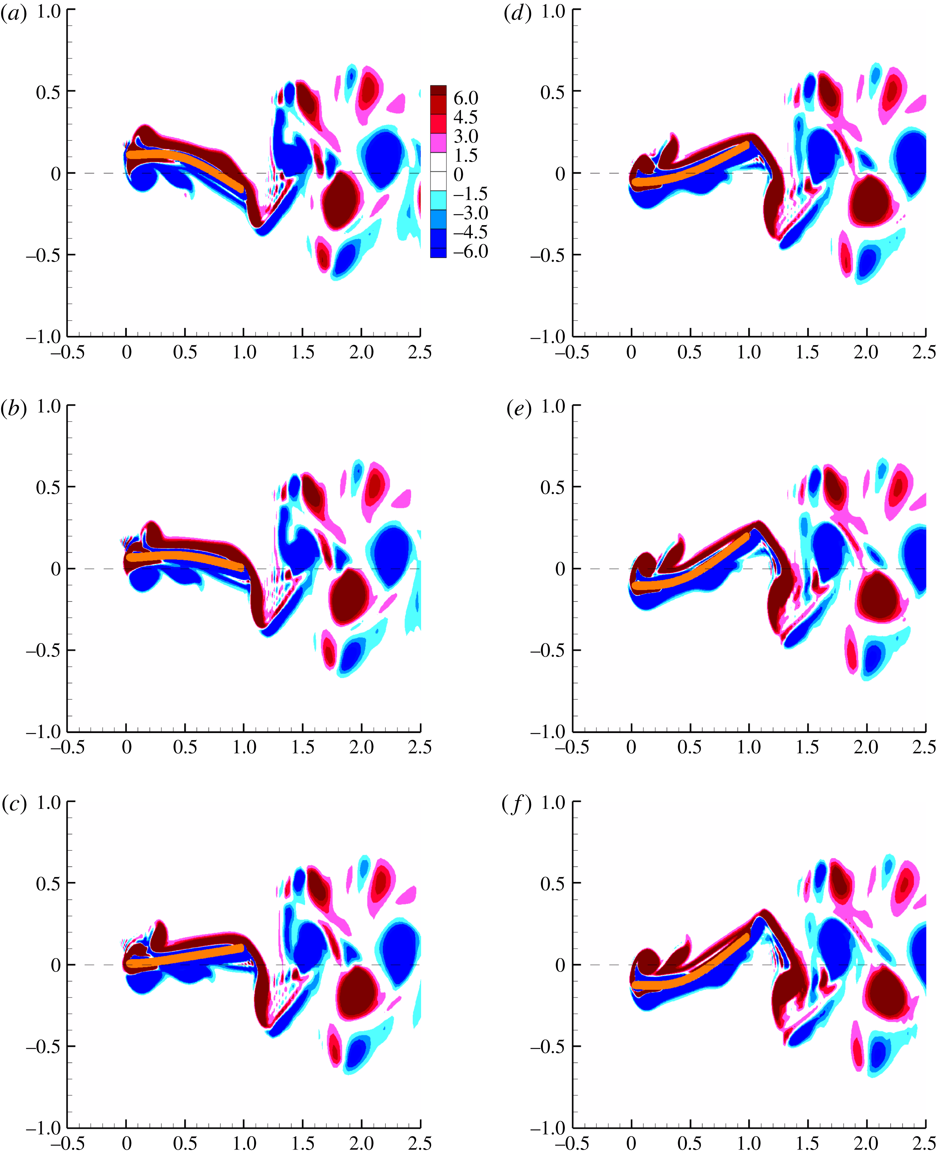
The snapshots of the vorticity around the foil are shown in figure 22. The deflection pattern of the foil is predominantly first mode with a weak contribution from the second mode. The wake vorticity pattern is a reverse von Kármán vortex street that is usually associated with thrust, even though the force in the free-stream direction computed from the pressure differential across the foil denotes drag. The leading-edge vortex is small and weak and shows separation very early on. In fact one notices in figure 22(d,f) that the leading-edge vortex is separated from the top surface of the foil and the adverse pressure gradient created by the positive slope and curvature of the foil deflection. One can observe a similar behaviour on the bottom surface in figure 22(a,c) but with a negative slope and curvature. In fact, if one were to compare the nature of the foil deflection at this frequency, as shown in figure 22(a,c,e) as the foil is executing a down stroke, it is opposite to that for the corresponding instances when
 $\bar{{\it\Omega}}=2$
– figure 9, or even
 $\bar{{\it\Omega}}=1$
– figure 21. This contrast reflects in the phase difference between the differential pressure and foil slope, as we discuss below. However, the point to note here is that the foil deflection is determined by its elastodynamics, which in turn is a function of the driving frequency
 $\bar{{\it\Omega}}=8.0$
. But if at this same frequency of oscillation one could, through distributed actuation, create a deflection shape similar to that of the foil oscillating at
 $\bar{{\it\Omega}}=2$
, then one could generate thrust rather than drag.
The differential pressure for
 $\bar{{\it\Omega}}=8.0$
, figure 23(a), shows pressure extrema at the leading edge of the foil due to the leading-edge vortex formation. There is a significant pressure differential at the trailing edge also, which is primarily due to high velocities and accelerations and is non-circulatory in nature. The pressure magnitude maxima is in fact higher to that for
 $\bar{{\it\Omega}}=2.0$
seen in figure 23(b), and these high pressure magnitudes are sustained over larger regions and longer times over the foil in one oscillation cycle. But, as we discuss next, it is the phase relation between pressure and foil slope that induces drag rather than thrust from the differential pressure that is generated across the foil surface.
Wake vorticity contours at
 $\bar{{\it\Omega}}=8.0$
and
 ${\it\mu}=0.33$
: (a)
 $\bar{{\it\Omega}}{\it\tau}={\rm\pi}/2$
; (b)
 $\bar{{\it\Omega}}{\it\tau}={\rm\pi}/2+{\rm\pi}/5$
; (c)
 $\bar{{\it\Omega}}{\it\tau}={\rm\pi}/2+2{\rm\pi}/5$
; (d)
 $\bar{{\it\Omega}}{\it\tau}={\rm\pi}/2+3{\rm\pi}/5$
; (e)
 $\bar{{\it\Omega}}{\it\tau}={\rm\pi}/2+4{\rm\pi}/5$
; (f)
 $\bar{{\it\Omega}}{\it\tau}=3{\rm\pi}/2$
.
Differential pressure for
 ${\it\mu}=0.33$
at
 $\bar{{\it\Omega}}=8.0$
(a) and
 $\bar{{\it\Omega}}=2.0$
(b).
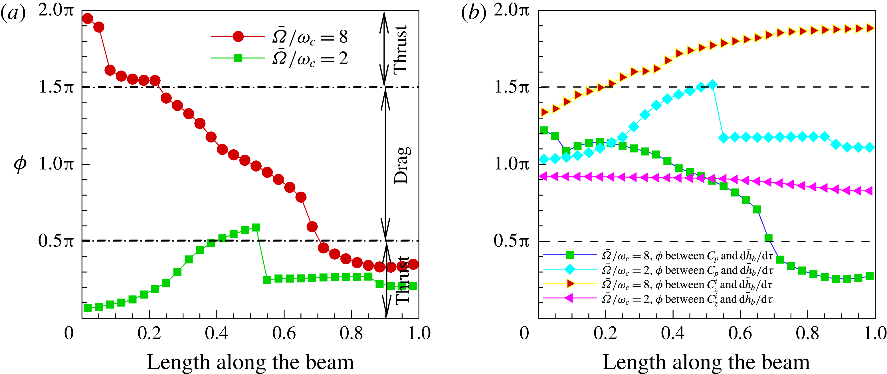
Phase difference
 ${\it\phi}$
between forces on the foil and foil kinematics for
 ${\it\mu}=0.33$
at
 $\bar{{\it\Omega}}=8.0$
and
 $\bar{{\it\Omega}}=2.0$
: (a) pressure and slope, (b) force and
 $\text{d}\bar{h}_{b}/\text{d}{\it\tau}$
.
Propulsive performance for
 $10\leqslant \bar{{\it\Omega}}\leqslant 30$
.
The phase difference between pressure and slope for
 $\bar{{\it\Omega}}=8.0$
, figure 24(a), clearly shows that the phase relation overall gives rise to drag. In the region
 $0<x/L\leqslant 0.05$
the phase angle is close to
 $0$
and the pressure contributes to thrust. Beyond,
 $0.05<x/L\leqslant 0.2$
, the phase angle is close to
 ${\rm\pi}/2$
and contributes almost no thrust. From
 $0.2<x/L\leqslant 0.7$
, the phase relation lies between
 ${\rm\pi}/2$
and
 $3{\rm\pi}/2$
and therefore drag is generated. From
 $x/L=0.7$
to the trailing edge the phase angle is close to
 ${\rm\pi}/2$
and very little thrust is created. So, overall, the differential pressure contributes to drag.
The phase relation between pressure and foil leading edge velocity – figure 24(b) – is such that overall energy is lost from elastic foil to surrounding fluid, whereas, in the case of the phase angle between inertia and foil leading-edge velocity is such that overall energy is added to the elastic solid by the inertia forces. So there is very little power input injected to the system, but since the pressure contributes to drag, the efficiency is strictly undefined.
4.2. Mode-II
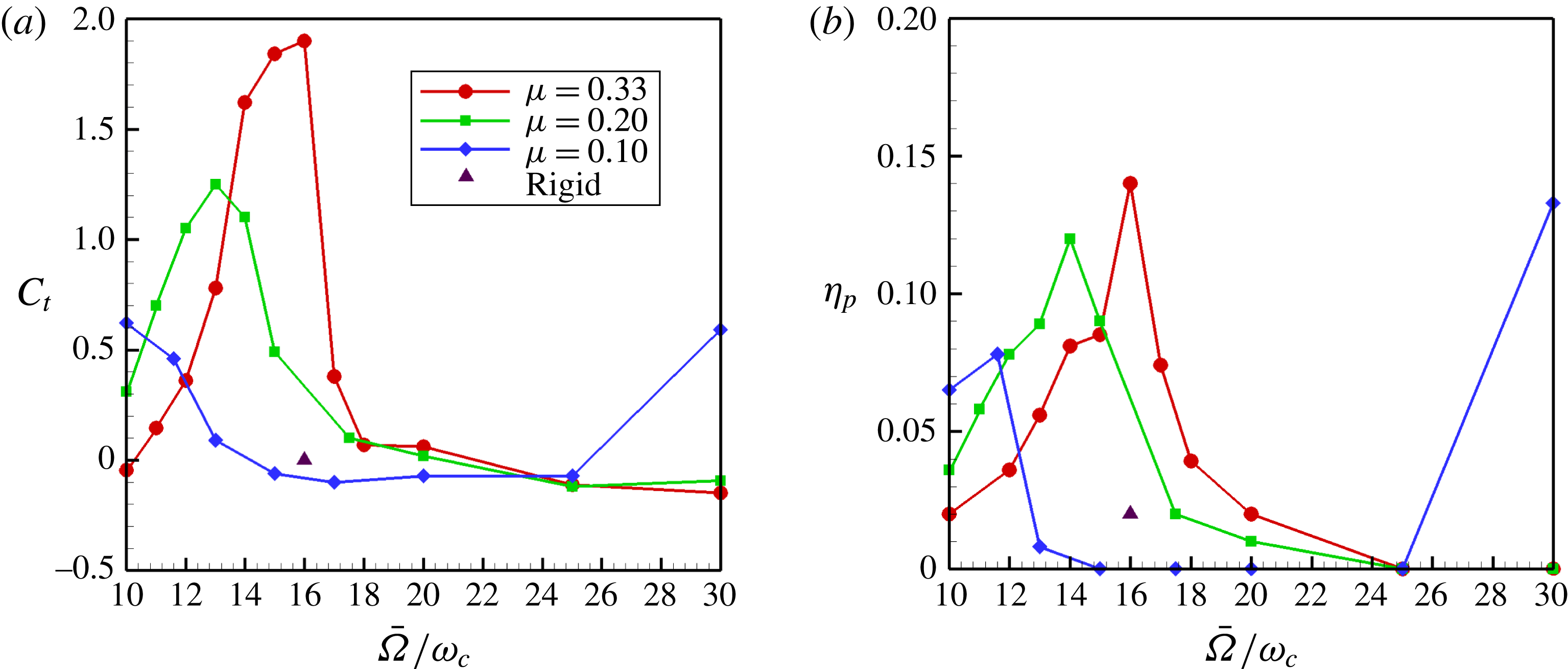
The thrust and propulsive efficiency in the frequency range
 $10<\bar{{\it\Omega}}\leqslant 30$
are shown in figure 25. The thrust and efficiency of an equivalent rigid foil is also shown in these figures, denoted by a solid triangle, at
 $\bar{{\it\Omega}}=16$
– the frequency at which maximum thrust and efficiency occur. The displacement profile in this range is a mix of first and second in-vacuum natural modes and figure 7(b) is a multiple exposure of deflection patterns at
 $\bar{{\it\Omega}}=16$
. In this frequency range, the thrust and efficiency levels decrease as the mass ratio falls. The frequencies at which the thrust and propulsive efficiency peak is also lower as the mass ratio decreases. We have observed that if the mass ratio were to be increased beyond
 ${\it\mu}=0.33$
, the frequency at which thrust and efficiency maxima occur approach that of the in-vacuum natural frequencies of the foil. This is reasonable as an increase in mass ratio implies that the motion of the solid dominates that of the fluid.
Wake vorticity contours at
 $\bar{{\it\Omega}}=16.0$
and
 ${\it\mu}=0.33$
. (a)
 $\bar{{\it\Omega}}{\it\tau}={\rm\pi}/2$
; (b)
 $\bar{{\it\Omega}}{\it\tau}={\rm\pi}/2+{\rm\pi}/5$
; (c)
 $\bar{{\it\Omega}}{\it\tau}={\rm\pi}/2+2{\rm\pi}/5$
; (d)
 $\bar{{\it\Omega}}{\it\tau}={\rm\pi}/2+3{\rm\pi}/5$
; (e)
 $\bar{{\it\Omega}}{\it\tau}={\rm\pi}/2+4{\rm\pi}/5$
; (f)
 $\bar{{\it\Omega}}{\it\tau}=3{\rm\pi}/2$
.
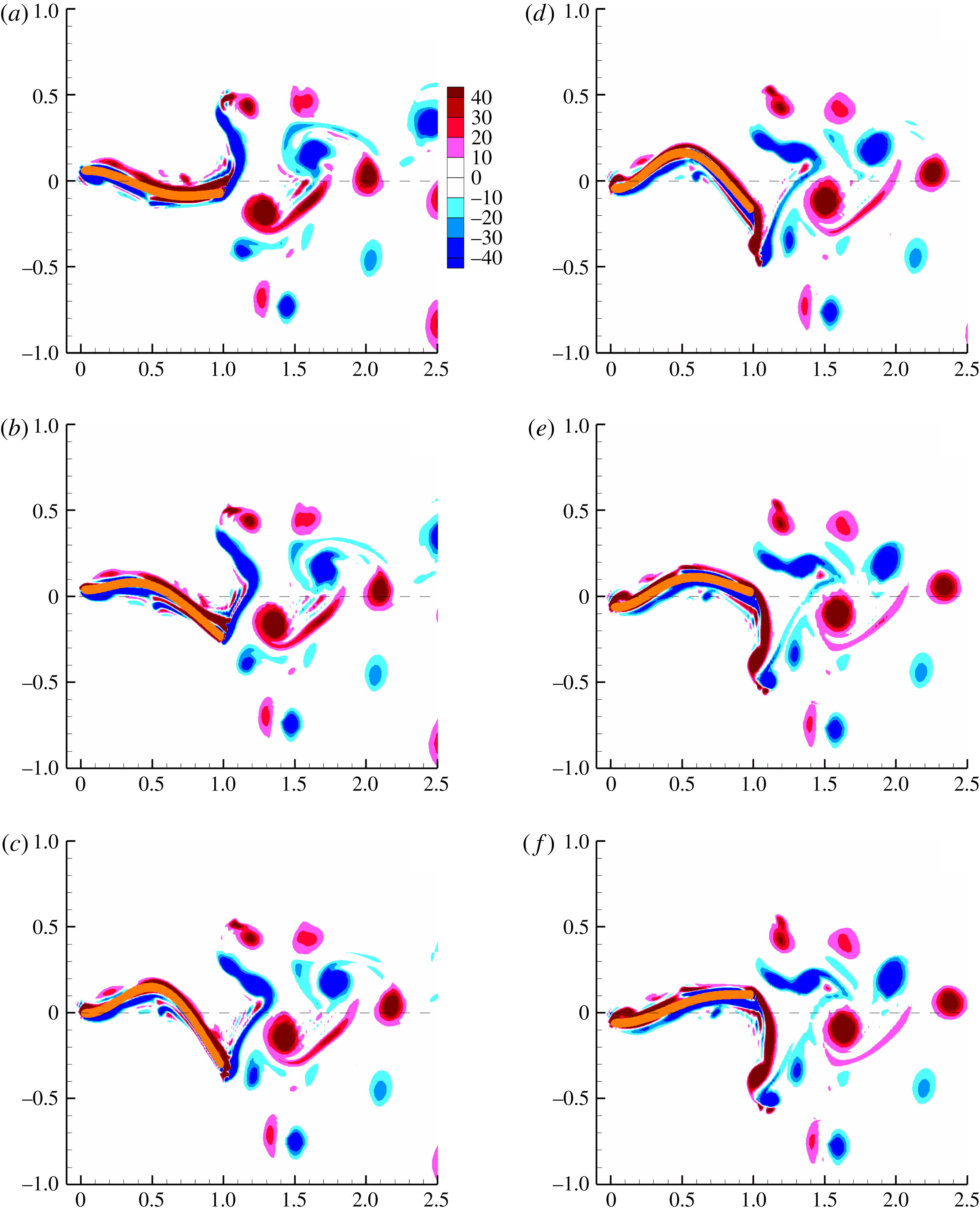
Figure 26 shows six snapshots of the vorticity contours over one half-period of the oscillating flexible foil at
 $\bar{{\it\Omega}}=16.0$
. A supplementary movie depicts the evolution and transport of vorticity as the flexible foil oscillates corresponding to the frequency
 $\bar{{\it\Omega}}=16$
. As we have set
 $\bar{{\it\Omega}}\bar{H}_{b}=1$
and the excitation frequency is high,
 $\bar{H}_{b}=1/16$
and small relative to when
 $\bar{{\it\Omega}}=1,2,\text{or even }8$
. The motion of the foil is from the top at the start of a down stroke – figure 26(a) – and the middle of the down stroke in figure 26(c). Figure 26(d–f) traces the vorticity and foil deflection in the remaining half of the down stroke that completes the half-cycle. One notices that the leading-edge vortex is very small and therefore its influence on pressure is very weak, primarily due to the high frequency and low amplitude of oscillation. There is a thin sheet of vorticity around the foil close to its surface. This sheet of vorticity breaks and shreds when the instantaneous slope of the foil changes sign. From figure 26(a) to 26(b) a small blob of vorticity near the mid-chord separates from the sheet of vorticity over the foil. This is caused by the large curvature of the foil near
 $x/L=0.6$
, as can be seen in the contour plots of the elastodynamics of the foil – figure 28(c,e). In figure 26(c,d), the sheet of vorticity originating from the leading edge to somewhere near the mid-chord separates, caused again by the large slope and curvature near the leading edge. In figure 26(d–f) there once again appears a leading-edge vortex coinciding with the reversal of sign of the slope and curvature. This completes the half-cycle. Two vortices of opposite sign are shed in one cycle of oscillation. The flow field is asymmetric.
In Quinn et al. (Reference Quinn, Lauder and Smits2014, figure 6(b)), a deflection pattern similar to ours is observed, though the vorticity field around the foil is quite different. One possible reason could be the low mass ratios –
 $10^{-2}$
to
 $10^{-4}$
– of the fluid–elastic system there. High mass ratios cause significantly higher inertia loading on the fluid as well as the foil, and together with changes in slope and curvature cause shredding or breaking of the vortical structures around the immediate vicinity of the foil. The other reason could be that in our simulations, the base or leading-edge excitation velocity
 $\bar{H}_{b}\bar{{\it\Omega}}=1$
, whereas in Quinn et al. (Reference Quinn, Lauder and Smits2014) the leading-edge displacement is fixed throughout the frequency range.
Comparison of pressure contours using viscous and potential fluid flow models for
 $\bar{{\it\Omega}}=16.0$
: (a) differential pressure – viscous, (b) differential pressure – potential.

In the pressure contour shown in figure 27(a) it appears as if the pressure maximum is moving from the trailing edge towards the leading edge over time, or that there is a backward propagating wave. The pressure computed from potential flow simulation is shown in figure 27(b) and shows a similar backward propagating wave. The pressure contour figure 27(a) shows high values between
 $0.2\leqslant x/L\leqslant 0.8$
and
 $0.8\leqslant x/L\leqslant 1.0$
but these are opposite in sign. With reference to the contour plots of the foil kinematics – figure 28 – all that we can infer is that the foil velocities and accelerations drive the differential pressure loading on the foil. Note that displacement, slope and curvature magnitudes are low relative to that of the velocities and accelerations. The slope and curvature though seem to influence the sign of the differential pressure on the foil.
Contours of elastodynamics and pressure for
 $\bar{{\it\Omega}}=16.0$
: (a) foil displacement, (b) foil acceleration, (c) foil slope, (d) foil angular velocity, (e) foil curvature, (f) foil angular acceleration.
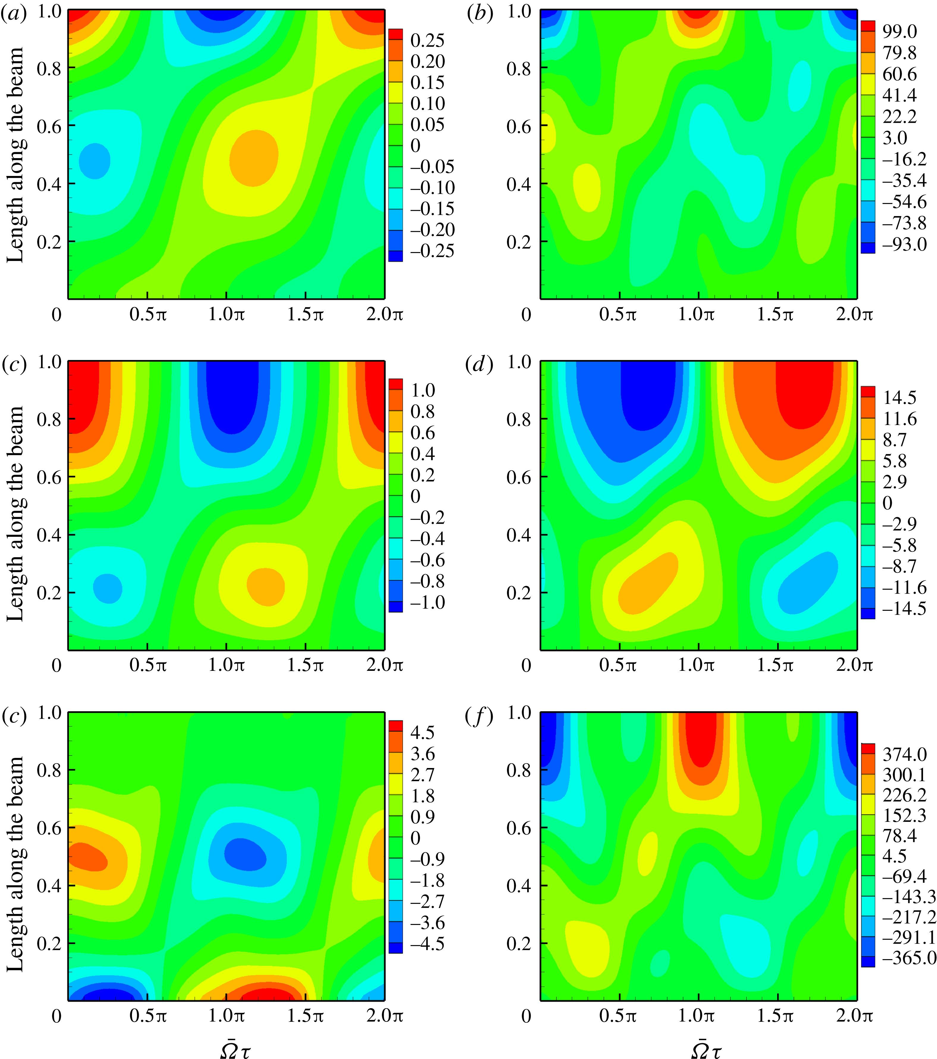
Figure 28 shows the contours of the elastodynamic response at
 $\bar{{\it\Omega}}=16.0$
. For high frequencies and with almost no leading-edge vortex formation, non-circulatory terms ought to dominate. Non-circulatory forces, for potential flow, and listed in § 4.1, are dependent on the angular velocity, angular acceleration and transverse acceleration. We have already noted in figure 27 that the pressure contours for viscous and potential flows are similar. The angular velocity figure 28(d), angular acceleration figure 28(f) and transverse acceleration are all high, in the region of
 $x/l=0.2$
,
 $0.4\leqslant x/L\leqslant 0.5$
, and from
 $0.6\leqslant x/L\leqslant 1.0$
. Note the magnitudes of the maxima; for the transverse acceleration it is
 $99.7$
, for the angular velocity it is
 $14.4$
and for the angular acceleration it is
 $374.6$
, all in non-dimensional units. The pressure differential across the foil, figure 27(a), is also high in the intervals on the foil where the angular velocity and acceleration and transverse acceleration are high.
Forces perpendicular and parallel to free stream for
 $\bar{{\it\Omega}}=16.0$
: (a) forces in the vertical direction, (b) forces in the free-stream direction.
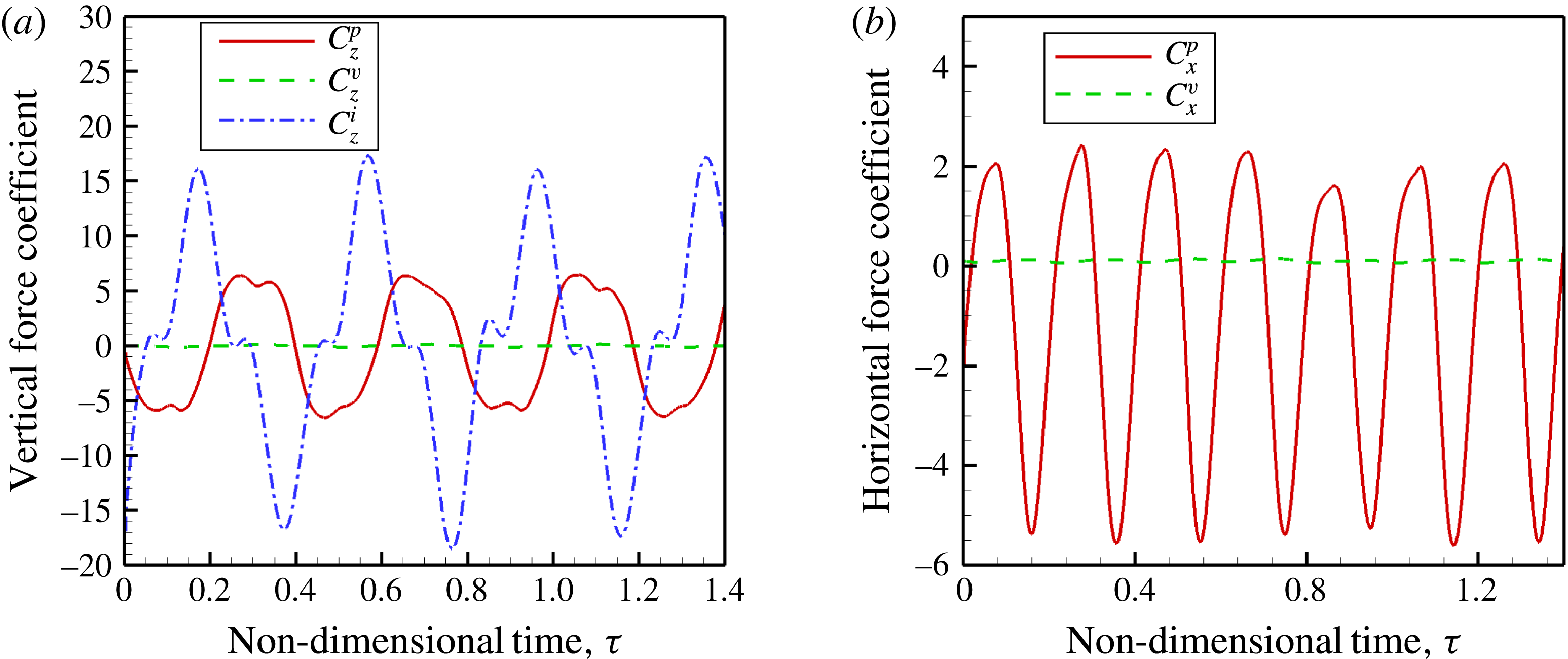
Figure 29 presents the forces perpendicular and parallel to free stream. The forces in the vertical direction, figure 29(a), are symmetric about the time axis and close to periodic; they almost sum to zero over one time period. In the free-stream direction figure 29(b), the viscous force contributes to drag, whereas the pressure force contributes to thrust over one time period. These forces are not strictly periodic as there are variations from cycle to cycle. The viscous forces are insignificant relative to the pressure and inertia forces.
Phase difference
 ${\it\phi}$
between forces on the foil and foil kinematics
 $\bar{{\it\Omega}}=16.0$
: (a) pressure and slope, (b) force and
 $\text{d}\bar{h}_{b}/\text{d}{\it\tau}$
.
Regions of thrust and drag on the foil
 $\bar{{\it\Omega}}=16.0$
.
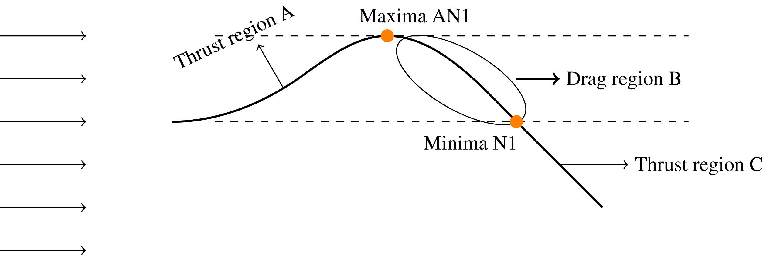
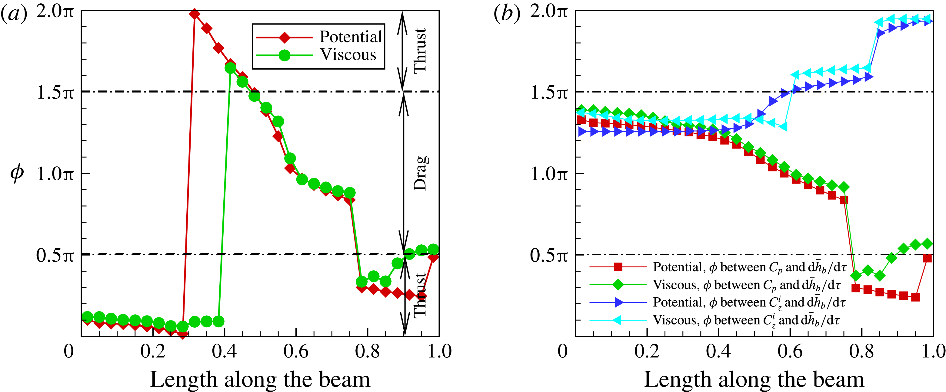
Figure 30(a) shows the phase difference between the pressure force and slope. The phase difference between pressure force and the slope lies in the thrust zone in the interval
 $0\leqslant x/L\leqslant 0.4$
;
 $x/L=0.5$
is the location of the displacement maxima on the foil – see figures 7(b) and 28(a). At
 $x/L=0.5$
the slope changes sign and we see that from this point that the phase difference is indicative of drag. This drag zone continues until
 $x/L=0.75$
. In the region from
 $x/L=0.75$
to the trailing edge, the pressure forces are found to contribute to thrust. A point to note is that potential and viscous flow simulations show almost identical variation that once again relates to the leading-edge vortex not influencing the pressure of the foil.
Figure 31 summarises the results of the pressure versus slope shown in figure 30(a). Positive slope associated with positive curvature denotes thrust and negative slope associated with negative curvature drag.
Figure 30(b) shows the phase difference between pressure and inertia force with base excitation heave velocity. The phase difference between the pressure force and the heave velocity is such that the work done by the pressure force is negative, or the elastic foil loses energy in doing work against pressure until close to
 $x/L=0.75$
. Beyond this point, until almost at the trailing edge, the fluid pressure force does positive work on the system. The phase difference between the inertia force and base excitation velocity is between
 ${\rm\pi}$
and
 $3{\rm\pi}/2$
from the leading edge to
 $x/L=0.6$
, thus negative work is done by the inertia forces on the system. Beyond this point, the inertia force does positive work on the elastic solid. Since pressure and inertia forces do positive work on the elastic foil towards the trailing edge of the foil, the energy supplied by the excitation mechanism is that much reduced, leading to high propulsive efficiency in the Mode-II frequency range at
 ${\it\mu}=0.33$
. But the efficiency in this frequency range is much lower in magnitude than that for Mode-I as there the frequencies themselves were low and the input power magnitudes lower, leading to even higher propulsive efficiencies.
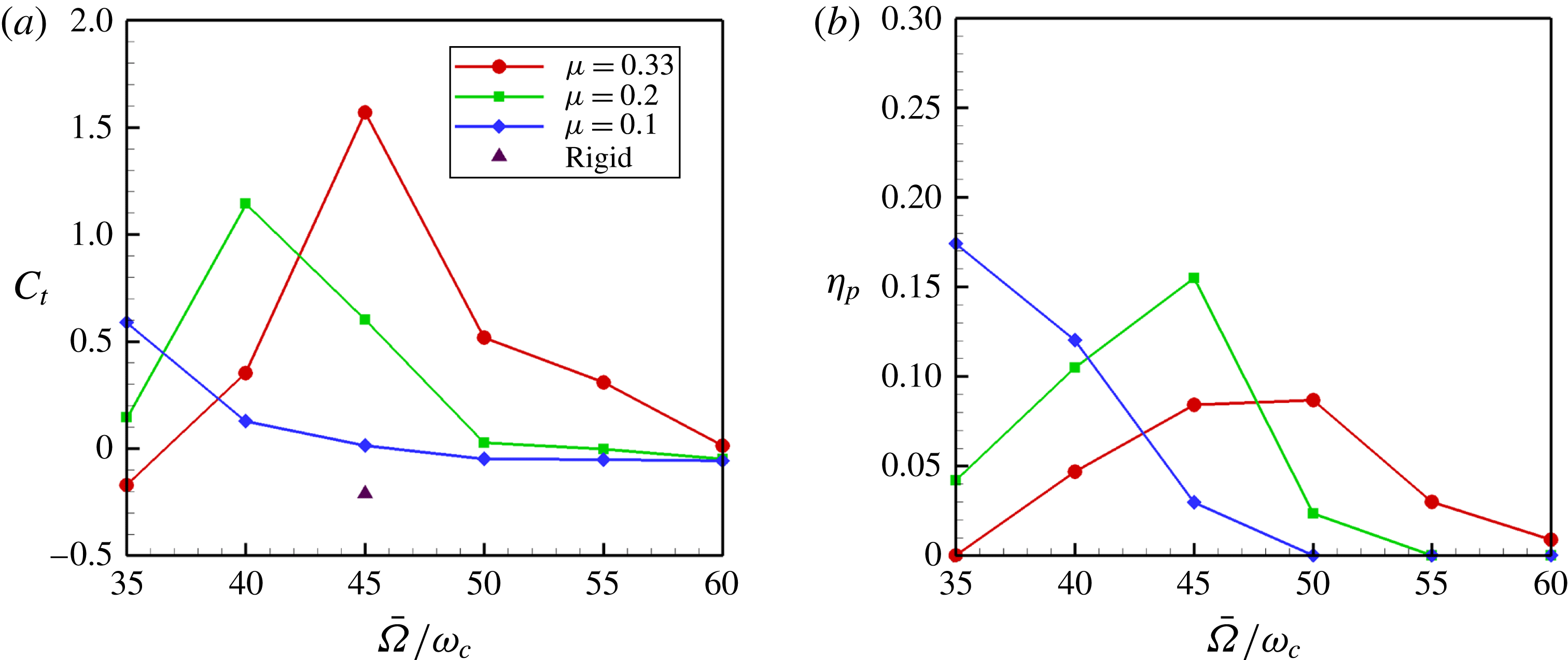
Propulsive performance for
 $35\leqslant \bar{{\it\Omega}}\leqslant 60$
.
4.3. Mode-III
The thrust and propulsive efficiency in this frequency range are shown magnified in figure 32. The maximum thrust coefficient occurs at
 $\bar{{\it\Omega}}=45.0,40.0,30.0$
for mass ratios
 $0.33$
,
 $0.2$
and
 $0.1$
, respectively. The propulsive efficiency is highest for
 ${\it\mu}=0.1$
, followed by
 ${\it\mu}=0.2$
and
 ${\it\mu}=0.33$
. For a given mass ratio, the maximum propulsive efficiency occurs at higher frequencies than where it occurs for the maximum thrust coefficient. For mass ratio
 $0.33$
, the maximum thrust coefficient occurs at
 $45.0$
and it is lower in value than the thrust coefficient at
 $\bar{{\it\Omega}}=16.0$
. For mass ratios
 $0.2$
and
 $0.1$
, the maximum thrust is observed at excitation frequencies
 $40.0$
and
 $30.0$
, respectively, which are lower than for
 ${\it\mu}=0.33$
. There are definite trends observed in the thrust coefficient and propulsive efficiency as a function of frequency and mass ratio in this regime. Heavier foils in a given fluid generate more thrust and lighter foils in the same fluid generate thrust more efficiently. The displacement of the foil for
 $\bar{{\it\Omega}}=45.0$
, figure 7(c), closely resembles the third in-vacuum natural mode. Unlike the deformation patterns for
 $\bar{{\it\Omega}}=2$
and
 $16$
, there is now a node close to the trailing edge.
Wake vorticity contours at
 $\bar{{\it\Omega}}=45.0$
and
 ${\it\mu}=0.33$
. (a)
 $\bar{{\it\Omega}}{\it\tau}={\rm\pi}/2$
; (b)
 $\bar{{\it\Omega}}{\it\tau}={\rm\pi}/2+{\rm\pi}/5$
; (c)
 $\bar{{\it\Omega}}{\it\tau}={\rm\pi}/2+2{\rm\pi}/5$
; (d)
 $\bar{{\it\Omega}}{\it\tau}={\rm\pi}/2+3{\rm\pi}/5$
; (e)
 $\bar{{\it\Omega}}{\it\tau}={\rm\pi}/2+4{\rm\pi}/5$
; (f)
 $\bar{{\it\Omega}}{\it\tau}=3{\rm\pi}/2$
.

Figure 33 shows six snapshots of vorticity contours around the foil in one half time period. A supplementary movie depicts the evolution and transport of vorticity as the flexible foil oscillates corresponding to the frequency
 $\bar{{\it\Omega}}=45$
. The wavelength of the wake is short due to the high frequency of shedding. Leading-edge vortex formation is very weak in this high frequency regime as the leading-edge displacement amplitude is very small given that we have fixed
 ${\it\Omega}H_{b}=1$
; one only observes shards of vorticity peeled away from the foil due to adverse pressure gradients created by the alternating signs of slope. A pair of vortices are shed in one cycle of oscillation and if one were to trace the path about which these vortices roll up, one observes a downward wake deflection.
Comparison of pressure contours using viscous and potential fluid flow models for
 $\bar{{\it\Omega}}=45.0$
: (a) differential pressure – viscous, (b) differential pressure – potential.
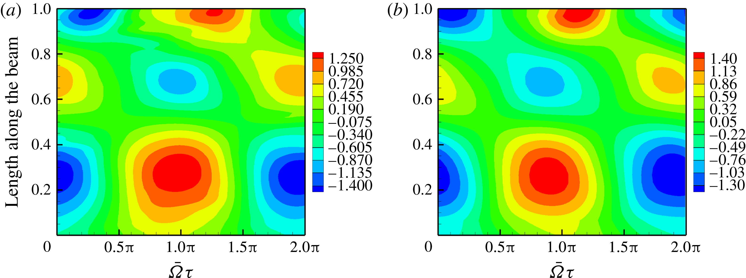
Figure 34(a) shows the pressure contour for viscous flow. The pressure computed from a potential flow simulation – figure 34(b) – is very close both qualitatively and quantitatively to that from the viscous simulation since there is no significant leading-edge vortex formation.
Contours of elastodynamics and pressure for
 $\bar{{\it\Omega}}=45.0$
: (a) foil displacement, (b) foil acceleration, (c) foil slope, (d) foil angular velocity, (e) foil curvature, (f) foil angular acceleration.
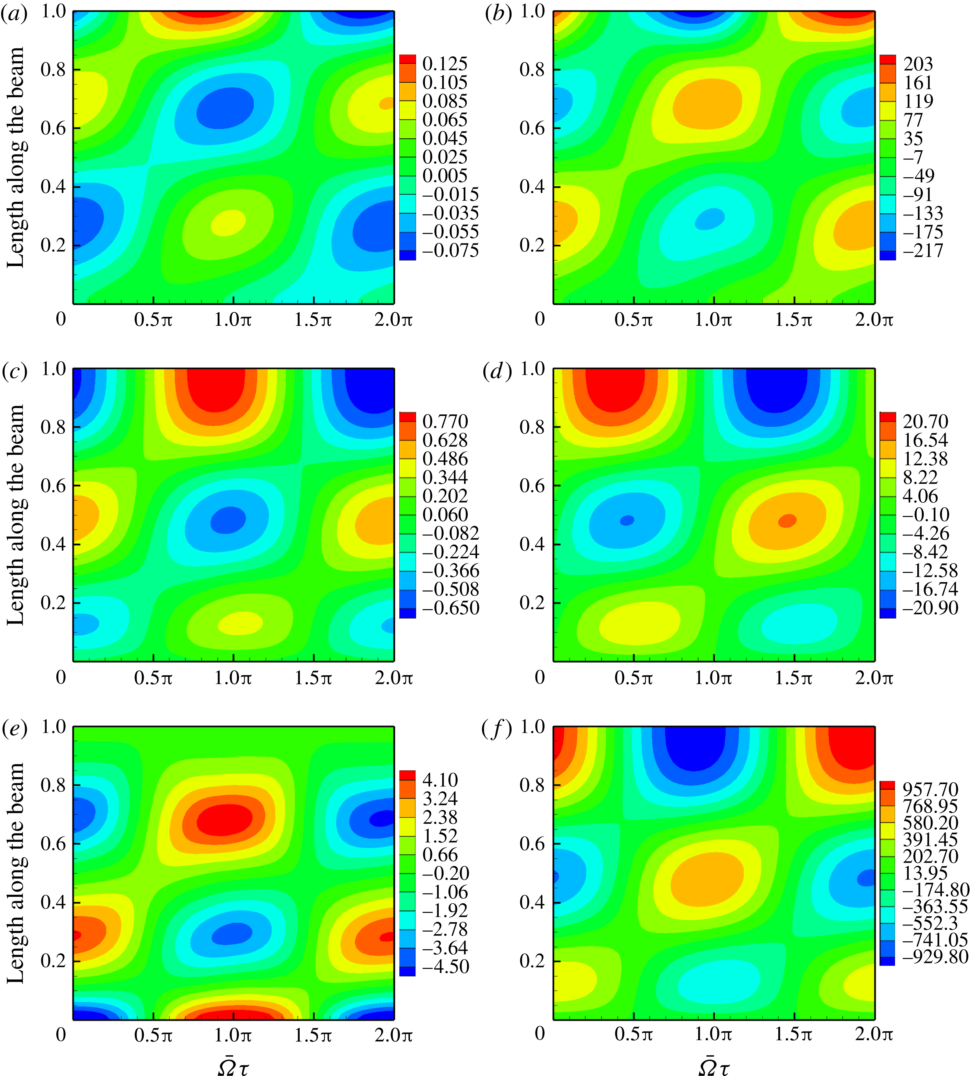
Figure 35 shows the contours of the elastodynamic response at
 $\bar{{\it\Omega}}=45.0$
. The figures in the right column correspond to acceleration and angular velocity, and if one were to compare them with the pressure contour shown in figure 34(a), it is easy to infer that pressure on the foil at this frequency is non-circulatory in origin. The magnitude of the non-dimensional velocities and accelerations are two orders of magnitude higher than the displacement, slope and curvature. Inertia, or non-circulatory, pressure terms dominate circulatory pressure terms. Of course, curvature and slope still determine the sign of vorticity besides having some influence on the pressure magnitude.
Forces perpendicular and parallel to free stream for
 $\bar{{\it\Omega}}=45.0$
: (a) forces in the vertical direction, (b) forces in the free-stream direction.
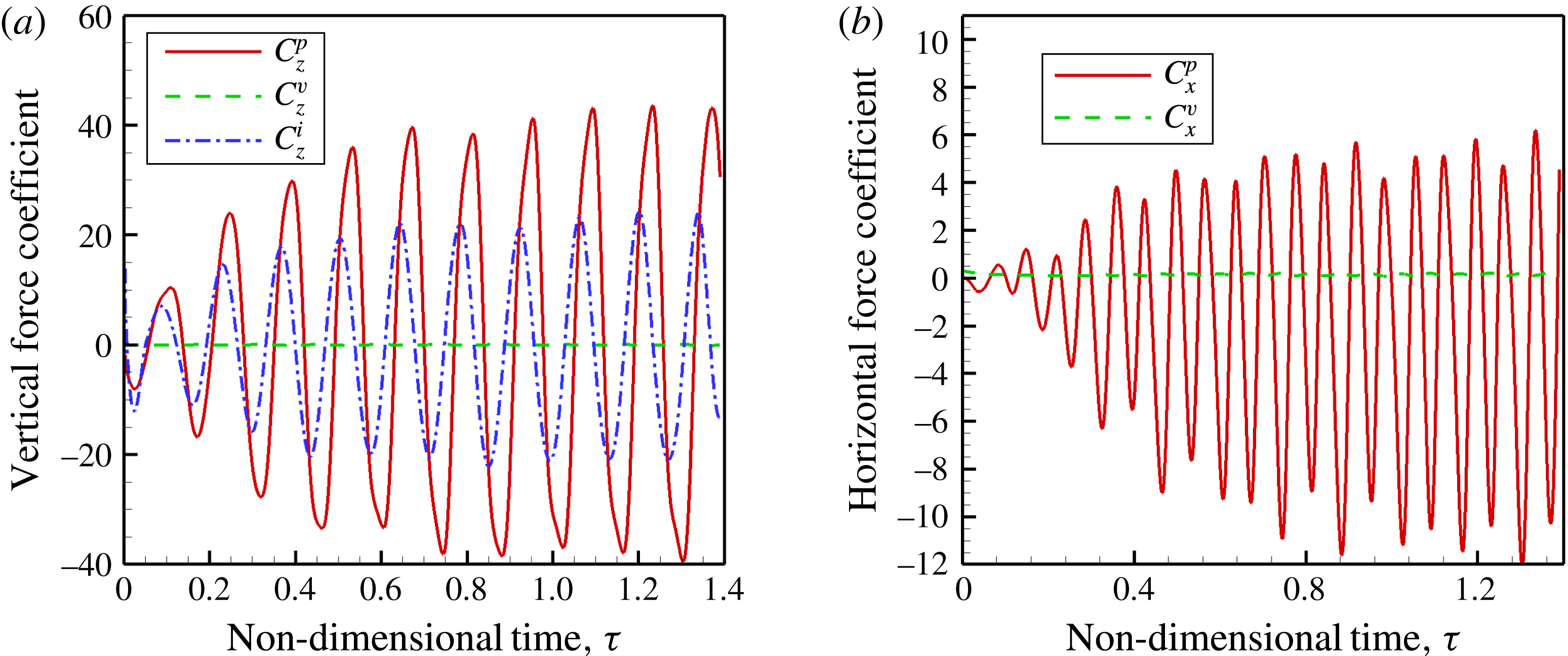
The forces in the direction perpendicular to the free stream are shown in figure 36(a). Once again, the viscous, pressure and inertial components give net zero lift averaged over one period. The forces are not periodic but are symmetric about the time axis. The forces in the free-stream direction that comprise thrust are shown in figure 36(b). Beyond the point where a steady state is reached, the thrust time history is aperiodic. In this case too, the viscous forces are insignificant relative to the pressure and inertia forces.
Phase difference
 ${\it\phi}$
between forces on the foil and foil kinematics
 $\bar{{\it\Omega}}=45.0$
: (a) pressure and slope, (b) force and
 $\text{d}\bar{h}_{b}/\text{d}{\it\tau}$
.

The phase difference between the pressure force and the slope is shown in figure 37(a). The phase difference variation should be read in conjunction with the deformation of the foil for this frequency, shown in figure 7(c), the pressure contour figure 34(a) and the elastodynamic contours in figure 35. From the leading edge until the first displacement maxima at
 $x/L=0.3$
, the phase difference between pressure and slope of the foil is close to
 $2{\rm\pi}$
and then falls to
 $3{\rm\pi}/2$
near the end of the interval, giving rise to thrust. The pressure reaches a maximum around
 $x/l=0.3$
, as shown in figure 34(a), but it contributes to drag as it is out-of-phase with the foil slope. Note that around
 $x/L=0.3$
the curvature is maximum and the slope changes sign. Thereafter, from
 $x/L=0.3$
to somewhere slightly aft of
 $x/L=0.5$
, the phase difference lies between
 $3{\rm\pi}/2$
and
 ${\rm\pi}/2$
, indicating drag. Close to
 $x/L=0.5$
, the slope is a local minima and the pressure is almost zero. Further aft along the foil, from
 $x/L=0.5$
to
 $x/L=0.7$
there is thrust. Note that the phase difference shifts from the interval
 $(0,{\rm\pi}/2)$
to
 $(3{\rm\pi}/2,2{\rm\pi})$
around
 $x/L=0.5$
. At
 $x/L=0.7$
, the foil curvature and acceleration as well as pressure are extrema. However, in the region
 $0.7<x/L<0.8$
, drag is mainly due to the adverse phase relation between pressure and slope. From
 $x/L=0.8$
until the trailing edge there is thrust and in this interval, the pressure is high because the acceleration and angular velocity are high. The thrust–drag pairs in the first four segments approximately cancel each other and it is only the segment near the trailing edge that contributes to thrust. This thrust is primarily generated by high accelerations of the foil and we therefore denote it as being non-circulatory in origin. Note that the phase relation between slope and pressure from the potential flow simulation, as also shown in figure 37(a), compare well with those of viscous flow simulations.
Regions of thrust and drag on the foil
 $\bar{{\it\Omega}}=45.0$
.
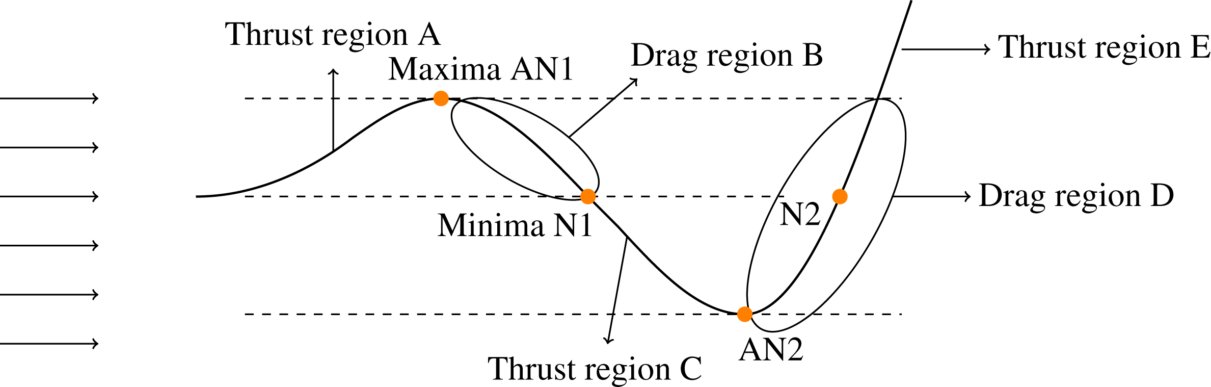
Figure 38 shows the shape of the airfoil at a particular instant for
 $\bar{{\it\Omega}}=45.0$
. The foil is divided into five parts, as against three parts for the mode-II regime. There exists three thrust regions A, C and E and two drag regions B and D. There exists two points AN1 and AN2 where the magnitude of displacement is a local extremum. Similarly, two points, N1 and N2, are present with local minimum displacement magnitude. Regions of thrust and drag correspond to those derived from the pressure versus slope variation (figure 37
a).
The phase difference between the pressure and inertia forces acting on the foil with reference to the base excitation velocity is shown in figure 37(b). The pressure force does negative work, or extracts energy from the elastic system, in the region starting from the leading edge to somewhere near
 $x/L=0.5$
. From
 $x/L=0.5$
to
 $x/L=0.8$
the pressure does work on the elastic system, or adds energy to it. From
 $x/L=0.8$
until the trailing edge the pressure force does negative work. The inertia force does negative work on the elastic system from the leading edge to
 $x/L=0.5$
, does positive work in the region from
 $x/L=0.5$
to
 $x/L=0.8$
and negative work from
 $x/L=0.8$
until the trailing edge. The overall energy deficit in the elastic system is made up of the input force
 $f_{b}(t)$
acting at the base of the foil. Thus, the propulsive efficiency is not very high as the input force has to compensate for the negative work done by the inertia and pressure forces. Note once again that the results from potential and viscous flow simulations compare well, implying that viscous effects are negligible in this high-frequency low-amplitude regime.
5. Fluid flow velocity and thrust
The variation along the flexible foil of the coefficient of thrust for the three excitation frequencies at
 ${\it\mu}=0.33$
, where thrust is maximum, are shown in figure 39(a). The thrust coefficient was determined at selected points on the foil and corresponds to
 $((1/T)\int _{0}^{T}f(x,t)\,\text{d}t)/(1/2{\it\rho}U_{\infty }^{2})$
. For
 $\bar{{\it\Omega}}=2$
, the thrust coefficient is positive throughout the length of the flexible foil, as described in figure 16. That there is thrust throughout the length of the foil was also indicated by the variation of phase difference between pressure and slope of the foil in figure 15(a). Also shown in figure 39(b) is the horizontal component of the fluid flow velocity close to the upper surface of the foil – at a distance of 4 % of chord length
 $L$
from the upper surface of the foil – for
 $\bar{{\it\Omega}}=2$
. This flow velocity decreases from near the leading edge to a minimum at around
 $0.3L$
– there it is actually a reverse flow. Note that this reverse flow exists between
 $0.2L$
and
 $0.5L$
. The reverse flow is due to the large leading-edge vortex formed as seen in the vorticity snapshots in figure 9. Also, though the fluid flow velocity at the trailing edge is relatively high, the thrust near the trailing edge is relatively low. This is due to the fact that the pressure is mainly non-circulatory in origin from the mid-chord to the leading edge, and this pressure increases with frequency; the frequency itself being low gives rise to a low thrust.
At
 $\bar{{\it\Omega}}=16$
, the horizontal component of the flow velocity is high at the trailing edge and so is the thrust. However, notice that this horizontal component of the flow velocity at the trailing edge at
 $\bar{{\it\Omega}}=16$
is lower than that at
 $\bar{{\it\Omega}}=45$
where the fluid velocity is maximum among these three frequencies. Now coming back to
 $\bar{{\it\Omega}}=16$
and figure 39(b), there is no flow reversal as the flow velocity never crosses zero, and consequently there is no separation. Thrust is generated until
 $0.4L$
, thereafter there is drag until
 $0.8L$
and then thrust once again until the trailing edge. The thrust variation correlates well with the pressure-slope phase-difference variation seen earlier in figure 30(a) as well as the schematic of thrust variation at this frequency sketched in figure 31. The fluid velocity component at
 $\bar{{\it\Omega}}=16$
is high near the leading edge and the trailing edge; in between, there are slight variations with the fluid velocity trough slightly out of phase with respect to that of the thrust.
Thrust and fluid velocity variation along the foil for
 ${\it\mu}=0.33$
at frequencies where the thrust is a maximum –
 $\bar{{\it\Omega}}=2,16,45$
: (a) thrust variation along the foil, (b) flow velocity variation along the foil.
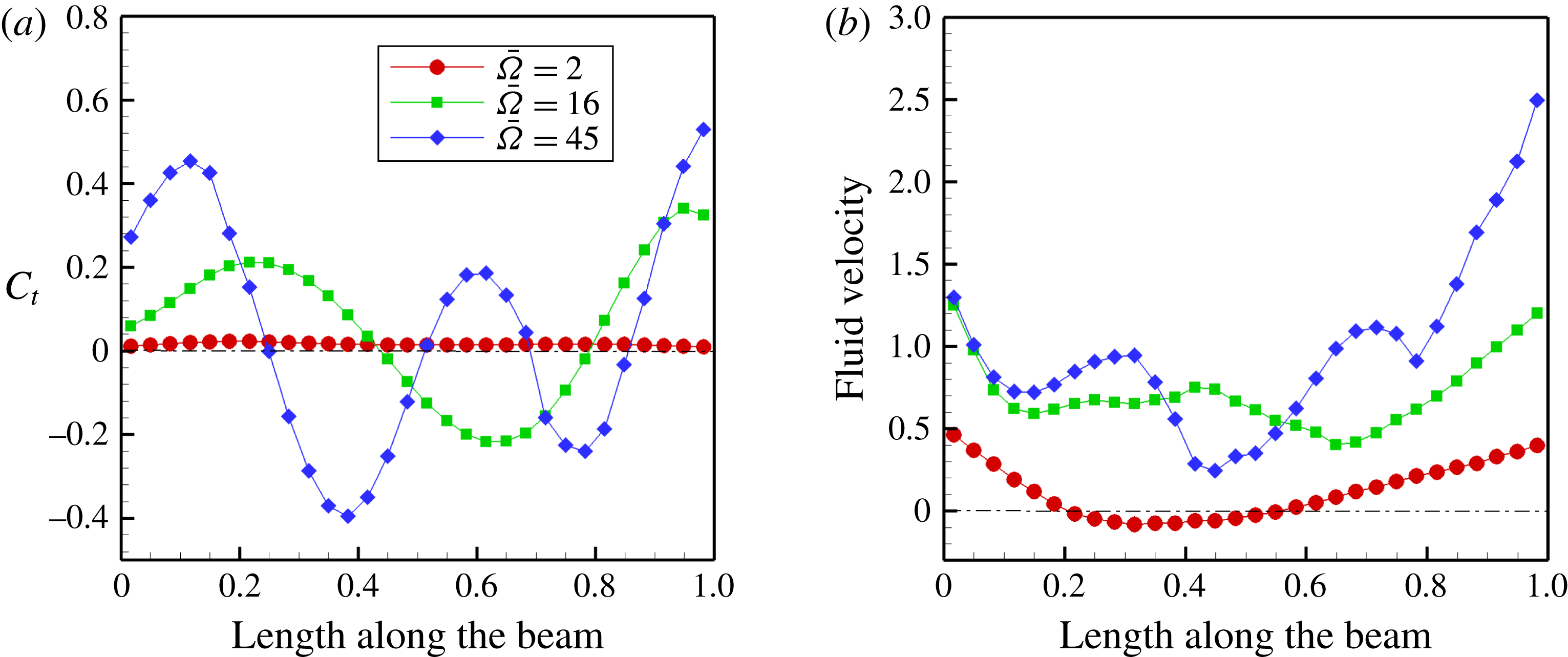
Thrust at
 $\bar{{\it\Omega}}=45$
correlates with the pressure-slope phase-difference variation – figure 37(a) – and the schematic of the thrust variation at this frequency – figure 38. The horizontal component of the velocity at the trailing edge is high relative to the other two frequencies and so is the horizontal component of the force at the foil trailing edge – the thrust. However, with reference to figure 5(a), the overall thrust at
 $\bar{{\it\Omega}}=45$
is lower than at
 $\bar{{\it\Omega}}=16$
due to the nature of the thrust variation along the length of the foil.
It was observed by Müller et al. (Reference Müller, Smit, Stamhuis and Videler2001, p. 2755) that the fluid velocity along the length of a swimming eel increases from head to tail, or leading edge to trailing edge. Therefore, it was conjectured that the thrust should increase continuously from leading edge to trailing edge. Neither of these are observed in our numerical simulations. In fact, there are alternating regions of thrust and drag along the foil that can be related to foil slope, curvature and velocities. Of course, one should keep in mind that the solid is modelled as one-dimensional here while that of the eel in Müller et al. (Reference Müller, Smit, Stamhuis and Videler2001) is a slender body of revolution; the fluid model is two-dimensional here while there it is three-dimensional.
Thrust coefficient
 $C_{t}$
and propulsive efficiency
 ${\it\eta}_{p}$
as a function of trailing-edge Strouhal number
 $St=(\bar{{\it\Omega}}(\bar{h}_{b}({\it\tau})+\bar{h}(1,{\it\tau}))_{max})/({\rm\pi}\bar{U}_{\infty })$
for different mass ratios
 ${\it\mu}$
: (a) thrust coefficient
 ${\it\mu}=0.1$
, (b) propulsive efficiency
 ${\it\mu}=0.1$
, (c) thrust coefficient
 ${\it\mu}=0.2$
, (d) propulsive efficiency
 ${\it\mu}=0.2$
, (e) thrust coefficient
 ${\it\mu}=0.33$
, (f) propulsive efficiency
 ${\it\mu}=0.33$
.
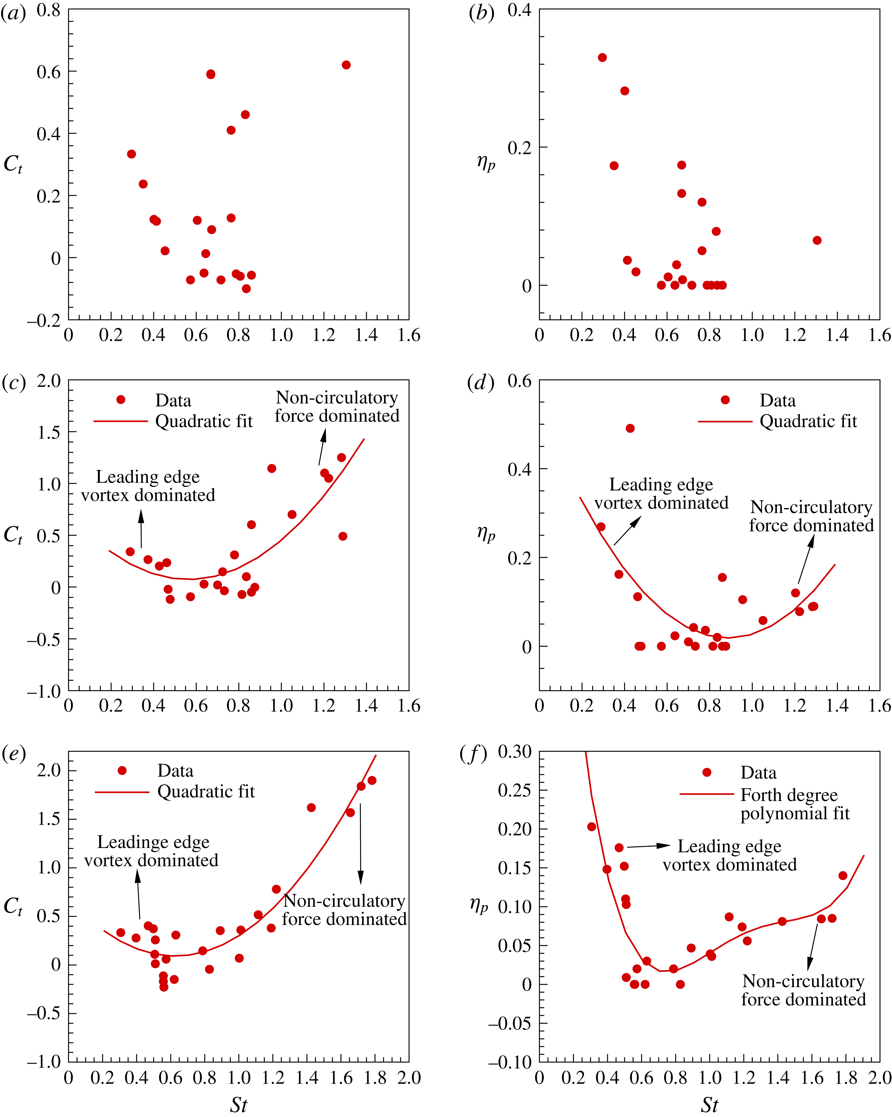
6. Thrust and efficiency and Strouhal number
In figure 5(c) of § 3, the variation of flexible foil trailing-edge velocity as a function of excitation frequency
 $\bar{{\it\Omega}}$
was shown. Barring the low frequency, or mode-I, frequency range, the scaled trailing-edge velocity maxima correlates well with the thrust maxima as indeed it should since thrust is largely due to the net momentum imparted to the fluid.
The Strouhal number
 $St=(\bar{{\it\Omega}}(\bar{h}_{b}({\it\tau})+\bar{h}(1,{\it\tau}))_{max})/({\rm\pi}\bar{U}_{\infty })$
is related to the trailing edge flapping velocity; in fact it is a rescaled trailing edge flapping velocity. The subscript refers to the maximum excursion of the trailing edge of the flexible foil from its undisturbed position coincident with the
 $x$
axis. Figure 40(a,c,e) shows thrust variation with respect to Strouhal number and the right-hand panels show propulsive efficiency variation. These results should be viewed in conjunction with those presented in figure 5(a–c). For a light foil, such as when
 ${\it\mu}=0.1$
, the value of the thrust coefficient itself is not very high, and there is no discernible trend in its variation with Strouhal number; note that between
 $St=0.3{-}0.8$
there are many instances where drag is generated. We attempted to fit a curve through these data points so that we could deduce a scaling relation; however, we could not arrive at one. For mass ratios
 ${\it\mu}=0.2$
and
 $0.33$
we were able to fit a quadratic curve through the data points; the thrust coefficient shows a quadratic variation with a minima around
 $St=0.5$
. Around
 $St=0.5$
one observes drag. Low Strouhal numbers are associated with low frequencies, and here the thrust is primarily due to leading-edge vortex formation and transport close to the flexible foil surface. High Strouhal numbers are associated with moderate and high frequencies of oscillation and the thrust is high primarily due to non-circulatory pressure.
The propulsive efficiency variation shown in figure 40 as a function of Strouhal number almost looks like a mirror image of the thrust coefficient variation, with high propulsive efficiency at low Strouhal numbers due to low frequencies and low input forces, and at high Strouhal numbers the propulsive efficiency gradually increases due to higher values of thrust.
Quinn et al. (Reference Quinn, Lauder and Smits2014, figure 13) showed that the averaged thrust coefficient increases parabolically as a function of the Strouhal number. We see an increase, but only beyond
 $St=0.6$
. Between Strouhal numbers
 $0.2$
and
 $0.6$
the thrust coefficient computed by us drops in value. The drop in value of the propulsive efficiency, in our case, occurs rather steeply, around
 $St=0.5$
. This discrepancy could be due to two reasons: one, the very low mass ratios –
 ${\sim}10^{-4}$
to
 $10^{-2}$
– of the fluid–elastic system used in the experiments conducted by Quinn et al. (Reference Quinn, Lauder and Smits2014); and the other, our experiments were simulated with constant heave velocity
 ${\it\Omega}\bar{H}_{b}=1$
, while those of Quinn et al. (Reference Quinn, Lauder and Smits2014) were performed at constant heave displacement amplitude
 $H_{b}=10~\text{mm}$
. We chose constant heave velocity as it is a commonly used parameter to characterize oscillations in heave or flapping (Lewin & Haj-Hariri Reference Lewin and Haj-Hariri2003).
7. Concluding remarks
Reviewing the analysis presented in the preceding pages, it is now quite clear that the elastodynamics of the flexible propulsor is intertwined with the fluid dynamics, or more specifically the vorticity dynamics; in hindsight it seems obvious that it ought to be so. Secondly, it seems that thrust and propulsive efficiency are contraposed not only in the fact that thrust or drag is determined by the phase relation between pressure and slope, and propulsive efficiency by its twin dependence on the phase relation between pressure and inertia forces and foil velocity, but also in their variations with frequency and Strouhal number. At low frequencies of oscillation, propulsive efficiencies are high aided by leading-edge vortices which remain attached as a consequence of favourable foil slope and curvature; thrust values however are quite low. The intermediate and high-frequency ranges seem to be the most appropriate if maximizing thrust generation is the criteria; propulsive efficiency though is low in these regimes. This fact is further reinforced by the almost mirror image nature of the variation of thrust and propulsive efficiency with Strouhal number.
Given the limitations of these numerical experiments, namely, two-dimensionality of the flow field, no spanwise deformation of the elastic solid, the flexible propulsor disturbed harmonically at the trailing edge rather than actuated continuously along the foil and the narrow range of mass ratios simulated, these results reveal interesting behaviour. One, in order to achieve high thrust, it is important that the phase difference between pressure and slope of the foil to be synchronous, or in other words, in phase. Achieving high propulsive efficiency requires in-phase behaviour of inertia and pressure forces with foil flapping velocity. Secondly, low frequencies and moderate-to-high amplitudes of heaving, together with synchronous pressure and slope, lead to moderate thrust and high propulsive efficiency derived from leading-edge vortex formation. So, rather than passive flapping, if one were to use active, continuous actuation along the foil length, one may be able to realise high thrust at moderately high propulsive efficiencies.
There are many questions and pointers that these results raise. One, what about the behaviour at lower, and perhaps higher, mass ratios than we have considered? In fact there is a need to tabulate the mass ratios of various avian and aquatic flapping propulsors that occur in nature. Then, the most obvious question would be the effect of finite aspect-ratio wings and three-dimensionality of the flows; how do these interact with flexibility and inertia? How do their vortical signatures look? How do they interact with the elastodynamics, and what are their influence on thrust and propulsive efficiency? Lastly, the lifting surface we used in our simulation was a flexible flat plate; it would be worthwhile to study wing sections that are optimized for low-Reynolds-number flows such as laminar flow airfoils.
Acknowledgements
This research was supported partially by a research grant on ‘A numerical study of vortex dynamics in flexible wing propulsors’ by the Asian Office of Aerospace Research and Development (AOARD), Tokyo Japan, on behalf of the U.S. Air Force Research Laboratory (AFRL). The authors gratefully acknowledge this support.
The authors would also like to record their appreciation to the reviewers for their comments and criticisms – the manuscript reads that much better.
Supplementary movies
Supplementary movies are available at http://dx.doi.org/10.1017/jfm.2015.659.
Appendix A. Validation of the flow solver
We validated our code with examples from the literature. The grid is a non-uniform structured grid and the flexible body is immersed in it.
A.1. Steady flow past a circular cylinder
The immersed boundary technique is used to solve the flow over a stationary cylinder for different Reynolds numbers. The flow remains steady up to a Reynolds number of
 $40$
, and for values greater than that the flow becomes unsteady. Here, we present the validation at Reynolds number
 $40$
. A domain size of
 $40d\times 40d$
is used for the simulation. The resolution of the grid length near the cylinder is
 $0.012d$
for the fine grid, which results in a grid size of
 $439\times 209$
.
 $d$
denotes the diameter of the cylinder.
Figure 41 shows the streamline plot over a cylinder for Reynolds number
 $40$
. The non-dimensional length of the blob as shown in figure 41 is given by
 $L_{w}/d$
, where
 $L_{w}$
is the actual length of the blob. Table 2 shows the comparison of blob length and coefficient of drag on a cylinder. The converged values with increasing grid size are
 $L_{w}/d=2.26$
and the coefficient of drag
 $C_{D}=1.56$
. These results are in good agreement with those reported in the literature (Ye et al.
Reference Ye, Mittal, Udaykumar and Shyy1993; Kim, Kim & Choi Reference Kim, Kim and Choi2001).
A.2. Steady flow past an airfoil
We also validated our code for steady flow over a NACA 0008 at an angle of attack of
 $4^{\circ }$
at
 $Re=2000$
. The flow is steady where a single vortex is shed and convected away in the wake. As the boundary layer is very thin at the leading edge, the grid size is very fine near the airfoil to resolve the boundary layer accurately. Three different grid sizes were used. The simulations were run until a steady state was reached. With the finest grid the calculated
 $C_{L}$
and
 $C_{D}$
values for the NACA 0008 airfoil at
 $Re=2000$
are
 $0.802$
and
 $0.274$
, respectively. The
 $C_{L}$
and
 $C_{D}$
values computed by us for different grid sizes, as well as those of other investigators, are presented in table 3. The results computed by us compare favourably with results from the literature (Kunz & Kroo Reference Kunz, Kroo and Meuller2001; Mittal et al.
Reference Mittal, Dong, Bozkurttas, Najjar, Vargas and von Loebbecke2008).
Streamline plot over a cylinder
 $Re=40$
.
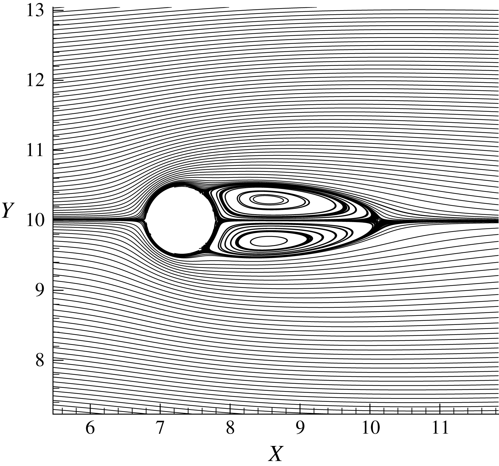
Comparison
 $L_{w}/D$
and
 $C_{D}$
over a cylinder
 $Re=40$
.
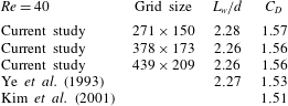
Comparison of
 $C_{D}$
and
 $C_{L}$
for NACA 0008 airfoil at
 ${\it\alpha}=4^{\circ }$
and
 $Re=2000$
.

Temporal variation of
 $C_{L}$
and
 $C_{D}$
: (a)
 $Re=300$
, (b)
 $Re=1000$
.

Vorticity contours around a cylinder: (a)
 $Re=300$
, (b)
 $Re=1000$
.
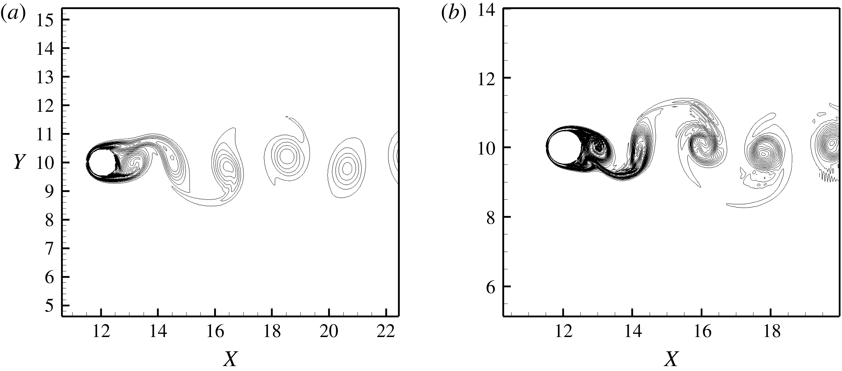
L2 norm residue variation with iteration number for pressure Poisson equation for flow over a cylinder at
 $Re=1000$
.
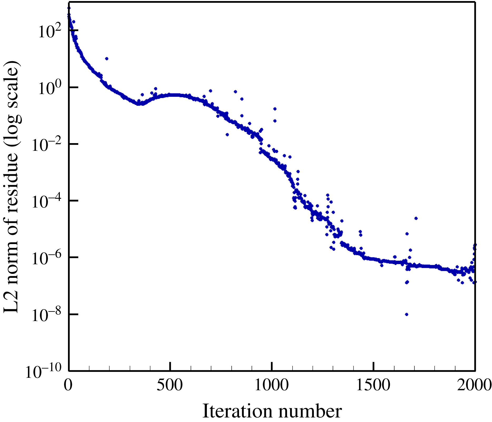
A.3. Unsteady flow past a circular cylinder
We now validate our code with an example involving unsteady flow over a stationary body. Flow over a cylinder above
 $Re=40$
yields unsteady flow. This unsteady flow leads to harmonic variations in the coefficients of lift and drag. Unsteady flow over a cylinder for Reynolds numbers of
 $300$
and
 $1000$
are studied. In the wake area, the grid is fine up to a length of
 $4d$
aft of the cylinder to resolve the wake accurately.
The temporal variation of instantaneous coefficient of lift and drag for Reynolds numbers
 $300$
and
 $1000$
are shown in figure 42(a,b), respectively. The vorticity contours are shown in figure 43(a,b) The Strouhal number is given by
 $St=(fd)/U_{\infty }$
where
 $f$
is the vortex-shedding frequency and
 $U_{\infty }$
is the free-stream velocity. Strouhal number and mean drag are calculated from the temporal variation of lift coefficient and drag coefficient plots. Tables 4 and 5 show the comparison of calculated Strouhal number and mean drag with results available in the literature (Williamson Reference Williamson1992; Henderson Reference Henderson1995; Mittal et al.
Reference Mittal, Dong, Bozkurttas, Najjar, Vargas and von Loebbecke2008) and our computed values compare well with those in the references cited.
The L2 norm of residue was considered for convergence for both Gauss–Sidel solver and preconditioned BI-CGSTAB solver. The convergence criteria was set to a residue value less than
 $10^{-6}$
. Figure 44 shows the variation of L2 norm of residue with iteration number for the discretized pressure Poisson equation for flow over a cylinder at
 $Re=1000$
.
Comparison of mean drag for cylinder
 $Re=300$
.
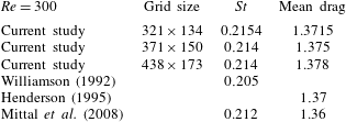
Comparison of mean drag for cylinder
 $Re=1000$
.
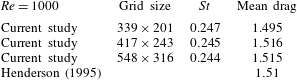
A.4. Unsteady flow past a heaving airfoil
We next study the example of a heaving airfoil in steady free-stream flow. The unsteady loads on the heaving symmetric Joukowski airfoil compared with the results of Lewin & Haj-Hariri (Reference Lewin and Haj-Hariri2003) for incompressible viscous flow. The rigid airfoil is undergoing prescribed periodic heaving motion with excitation frequency
 ${\it\Omega}$
in an incompressible viscous flow with constant free-stream velocity
 $U_{\infty }$
. The output power is calculated for reduced frequency of
 $k=5.33$
for
 $k\bar{H}_{b}=1.0$
. The non-dimensional heaving amplitude is
 $\bar{H}_{b}$
and the reduced frequency is given by
 ${\it\Omega}L/U_{\infty }$
, the Reynolds number is
 $500$
. The finest grid size is
 $309\times 223$
and table 6 lists the grid convergence study for the coefficient of lift. Figure 45 shows the comparison of temporal variation of output power with Lewin & Haj-Hariri (Reference Lewin and Haj-Hariri2003).
Temporal variation of output power,
 $P_{o}$
, over a heaving airfoil,
 $Re=500$
.
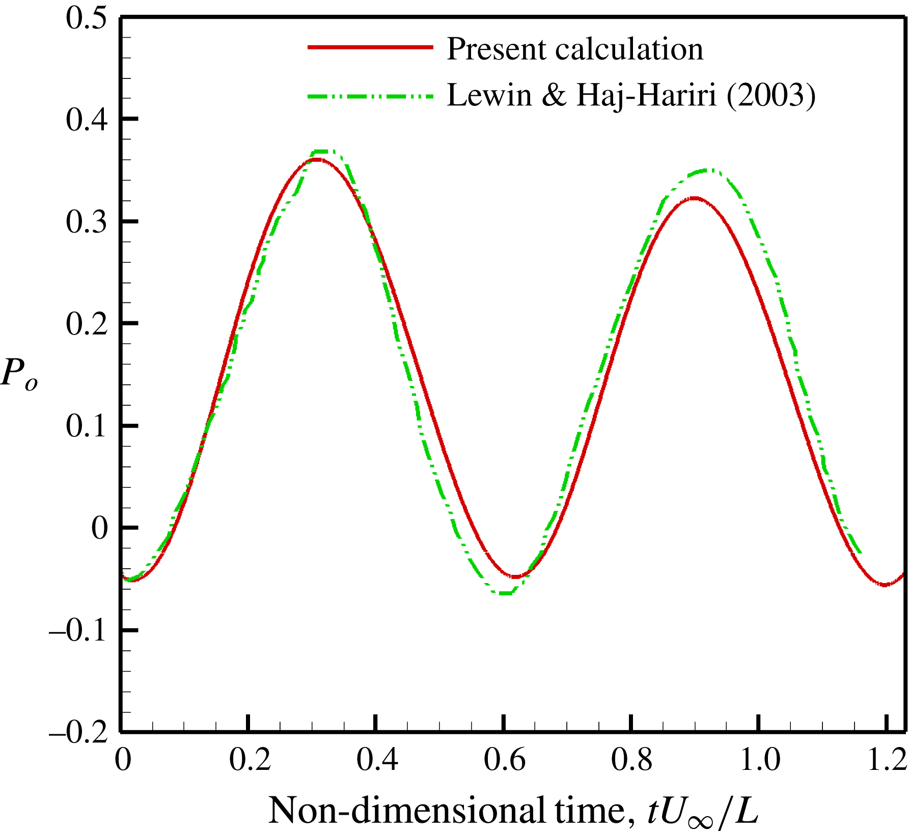
Grid convergence for unsteady Joukowski airfoil.
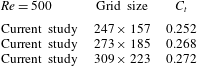
A.5. Flexible foil in an incompressible viscous flow
The equation of motion of the elastic vibration of the foil, given by (2.1), is discretized using the finite element method. In matrix notation
 $$\begin{eqnarray}\unicode[STIX]{x1D648}\ddot{\boldsymbol{u}}(t)+\unicode[STIX]{x1D63E}\dot{\boldsymbol{u}}(t)+\unicode[STIX]{x1D646}\boldsymbol{u}(t)=\boldsymbol{f}_{I}(t)+\boldsymbol{f}_{FL}(t).\end{eqnarray}$$
In the above,
 $\unicode[STIX]{x1D648}$
is the mass matrix,
 $\unicode[STIX]{x1D63E}$
is the strain rate proportional damping matrix and
 $\unicode[STIX]{x1D646}$
is the flexural stiffness matrix. Also,
 $\boldsymbol{f}_{I}(t)$
is the vector of inertia force at the nodes of the finite element model. Likewise,
 $\boldsymbol{f}_{FL}(t)$
is the vector of pressure forces. Finally,
 $\boldsymbol{u}(t)$
is the vector of nodal displacements. Details on the development of the finite element model are given in Clough & Penzien (Reference Clough and Penzien1993).
Free-vibration convergence studies on the foil.

The number of finite elements for modelling the flexible foil elastodynamics was chosen to be equal to the number of discrete vortex panels –
 $30$
in number. This was chosen on the basis of convergence studies on free vibration, as well as fluid dynamic tests for some text-book examples. For the elastodynamics of the foil, the number of elements are considered such that the first ten natural modes of the cantilevered beam are accurately captured and included in the response. Convergence testing was done up to the tenth mode by varying the number of finite elements. Figure 46(a) shows the variation of the frequency for the tenth mode of a cantilevered Euler–Bernoulli beam with respect to number of finite elements in the model. The percentage change in frequency of the tenth mode was less than 0.1 % at
 $30$
finite elements when compared with
 $35$
finite elements. Therefore,
 $30$
finite elements was chosen to model the elastodynamics. Figure 46(b) shows the comparison of frequencies of first ten natural modes of the cantilevered Euler–Bernoulli beam
 $30$
finite elements and an analytical approach presented in Bisplinghoff, Ashley & Halfman (Reference Bisplinghoff, Ashley and Halfman1955, pp. 75–77). The time step was chosen carefully such that it was less than the 20th part of the tenth natural mode time period of the flexible foil.
The coupled problem of fluid–elasticity is numerically solved using a predictor–corrector type algorithm. Let us assume that we have the solution at time
 $t_{n}$
. That is, we know the displacement, velocity and acceleration of the foil at time
 $t_{n}$
, as well as the pressure differential across the foil. We wish to compute the same at time
 $t_{n+1}$
. We start with an initial or assumed estimate of the solution at time
 $t_{n+1}$
, which we label with a subscript
 $a$
. The initial assumed displacement, velocity and acceleration of the foil for the
 $t_{n+1}$
time step are
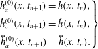 $$\begin{eqnarray}\left.\begin{array}{@{}c@{}}h_{a}^{(0)}(x,t_{n+1})=h(x,t_{n}),\\ {\dot{h}}_{a}^{(0)}(x,t_{n+1})={\dot{h}}(x,t_{n}),\\ \ddot{h}_{a}^{(0)}(x,t_{n+1})=\ddot{h}(x,t_{n}).\end{array}\right\}\end{eqnarray}$$
We now compute the pressure differential using these initial estimates of the displacement, velocity and acceleration at time step
 $t_{n+1}$
. Let the initial estimate, denoted by a subscript
 $e$
, of the pressure differential be
 ${\rm\Delta}p_{e}^{(0)}(x,t_{n+1})$
. Using the initial estimate of the pressure differential across the foil
 ${\rm\Delta}p_{e}^{(0)}(x,t_{n+1})$
, we compute the displacement and velocity and acceleration of the foil. We label these estimated values of the foil motion also with a subscript
 $e$
. That is
 $h_{e}^{(0)}(x,t_{n+1})$
,
 ${\dot{h}}_{e}^{(0)}(x,t_{n+1})$
, and
 $\ddot{h}_{e}^{(0)}(x,t_{n+1})$
. We then compare the assumed and estimated values of the motion parameters of the foil. In case they are within a prescribed error bound, then we terminate the iteration and proceed to the next time step. If they are not within the error bound, then we proceed to the next step in the iteration as
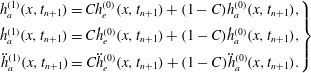 $$\begin{eqnarray}\left.\begin{array}{@{}c@{}}h_{a}^{(1)}(x,t_{n+1})=Ch_{e}^{(0)}(x,t_{n+1})+(1-C)h_{a}^{(0)}(x,t_{n+1}),\\ {\dot{h}}_{a}^{(1)}(x,t_{n+1})=C{\dot{h}}_{e}^{(0)}(x,t_{n+1})+(1-C){\dot{h}}_{a}^{(0)}(x,t_{n+1}),\\ \ddot{h}_{a}^{(1)}(x,t_{n+1})=C\ddot{h}_{e}^{(0)}(x,t_{n+1})+(1-C)\ddot{h}_{a}^{(0)}(x,t_{n+1}).\end{array}\right\}\end{eqnarray}$$
One then proceeds to compute the pressure differential as before for this iteration step within the
 $t_{n+1}$
time step. That is
 ${\rm\Delta}p_{e}^{(1)}(x,t_{n+1})$
. In general
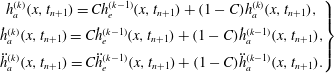 $$\begin{eqnarray}\left.\begin{array}{@{}c@{}}h_{a}^{(k)}(x,t_{n+1})=Ch_{e}^{(k-1)}(x,t_{n+1})+(1-C)h_{a}^{(k)}(x,t_{n+1}),\\ {\dot{h}}_{a}^{(k)}(x,t_{n+1})=C{\dot{h}}_{e}^{(k-1)}(x,t_{n+1})+(1-C){\dot{h}}_{a}^{(k-1)}(x,t_{n+1}),\\ \ddot{h}_{a}^{(k)}(x,t_{n+1})=C\ddot{h}_{e}^{(k-1)}(x,t_{n+1})+(1-C)\ddot{h}_{a}^{(k-1)}(x,t_{n+1}).\end{array}\right\}\end{eqnarray}$$
The value of
 $C$
lies between
 $0$
and
 $1$
and is chosen by trial and error. In the present simulation,
 $C=0.9$
ensures convergence within 1 %, in two iterations.
Grid independence study;
 $\bar{U}_{\infty }=1,\bar{{\it\Omega}}=16,{\it\mu}=0.33$
. (a)
 $C_{x}$
, (b)
 $C_{z}$
.
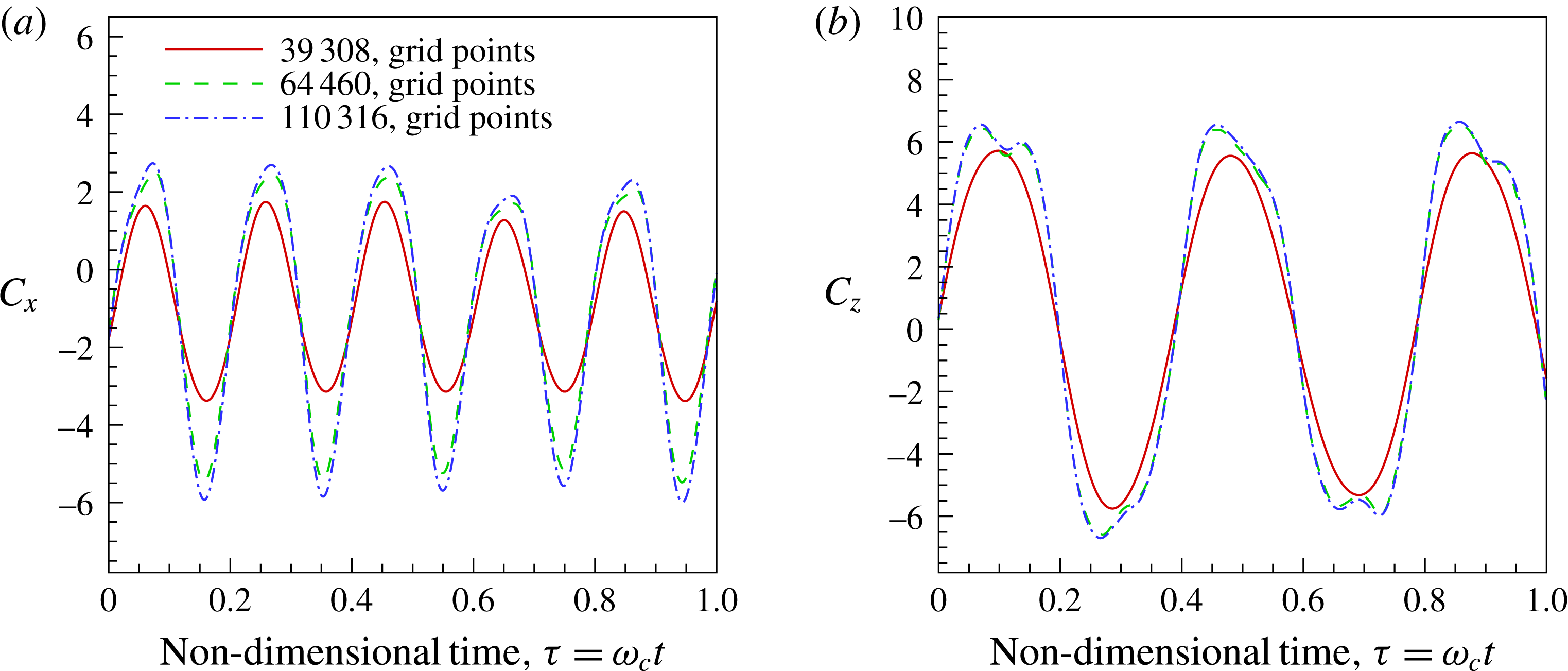
For numerical simulations involving a flexible one-dimensional foil in a two-dimensional incompressible viscous flow, the grid was finely resolved in the region where the motion of the body occurs. In the horizontal direction, the smallest size was
 $0.01$
in a region where the foil is present. The smallest cell size chosen near the airfoil boundary in the vertical direction was based on the frequency of heaving motion and varied gradually away from the foil. Typically the grid size increment is 10 % of the previous cell size. The grid size in the region aft of the foil where the wake is captured is
 $0.02$
of chord length. As the excitation frequency increased, care was taken in reducing the grid size in the vertical direction to capture the fast variation of boundary conditions in the vertical direction. For excitation frequencies
 $1<\bar{{\it\Omega}}<5$
, the smallest cell size in the vertical direction was
 $0.01$
, whereas for frequencies
 $5<\bar{{\it\Omega}}<25$
the smallest grid size was
 $0.0075$
and for frequencies
 $25<\bar{{\it\Omega}}<60$
the smallest size was
 $0.006$
. The far-field boundary was defined
 $8$
chord lengths away downstream and
 $4$
chord lengths upstream. In the vertical direction, the far field was
 $5$
chord lengths above and below the foil. Care was taken that the grid size was gradually increased towards the outer boundary.
The grid independence study was performed at different frequencies of heaving oscillations of the foil. We present the results of one such simulation when
 $\bar{U}_{\infty }=1,\bar{{\it\Omega}}=16,{\it\mu}=0.33$
– figure 47. The maximum error in the results for the grid size 64 460 with that of 110 316 was 6.5 % for
 $C_{x}$
and 2.5 % for
 $C_{z}$
. Given these values all simulations were done with a grid size of 64 460.



