





1 Introduction
Frequencies of radiocarbon determinations are now a standard tool for describing the tempo of past human and environmental activity. Summed calibrated probability distributions (SPDs) and kernel density estimates (KDEs) are routinely used to visualise peaks and troughs in dated events and to infer temporal phases of occupation, construction or ritual activity (e.g., Timpson et al. Reference Timpson, Colledge, Crema, Edinborough, Kerig, Manning, Thomas and Shennan2014; Bevan and Crema Reference Bevan and Crema2021; Mendez-Quiros et al. Reference Mendez-Quiros, Barceló, Santana-Sagredo and Uribe2023). Yet these inferences typically rely on informal visual inspection, with peaks and gaps identified by eye. Such approaches are vulnerable to sampling variability, taphonomic loss and structure in the calibration curve, and they are further affected by choices of temporal aggregation, smoothing and inclusion criteria (Contreras and Meadows Reference Contreras and Meadows2014; Surovell et al. Reference Surovell, Finley, Smith, Brantingham and Kelly2009; Crema Reference Crema2022).
Recent reviews emphasise that radiocarbon-frequency methods fall into three broad families: (i) reconstructive approaches, which estimate a smoothed intensity function over time (e.g., SPDs, KDEs, mixture models); (ii) hypothesis-testing frameworks, which use Monte Carlo or permutation procedures to test specific models against null expectations; and (iii) explicit model-fitting strategies, including Poisson and Cox-process models in likelihood or Bayesian form (Crema and Bevan Reference Crema and Bevan2021; Crema Reference Crema2022; Heaton et al. Reference Heaton, Al-assam and Bard2025; de Navascués et al. Reference de Navascués, Burgarella and Jakobsson2025). In this view, SPDs and KDEs are reconstructions of an underlying event intensity, not direct measurements of population size (Bronk Ramsey Reference Bronk Ramsey2017). They do not, by themselves, provide probabilistic statements about the number, timing or magnitude of discrete episodes.
A central practical problem is therefore segmentation: given a smoothed time series of dated activity, under what conditions is it defensible to treat peaks and troughs as distinct episodes? Archaeologists already use an implicit segmentation procedure when they mark off “phases” on an SPD or KDE plot (e.g., Bevan and Crema Reference Bevan and Crema2021; Timpson et al. Reference Timpson, Colledge, Crema, Edinborough, Kerig, Manning, Thomas and Shennan2014; Mendez-Quiros et al. Reference Mendez-Quiros, Barceló, Santana-Sagredo and Uribe2023). However, the criteria behind such decisions are rarely stated, and their performance has not been systematically evaluated with controlled simulations (Contreras and Meadows Reference Contreras and Meadows2014; Crema Reference Crema2022).
This paper proposes a simple and deliberately conservative segmentation rule: a Monte Carlo KDE–minima procedure that identifies activity pulses as contiguous calendar intervals between persistent minima of an ensemble of KDEs. The method is designed to sit within the reconstructive family of approaches. It formalises a familiar visual practice—reading episodes off a smoothed curve—without introducing the strong parametric assumptions of fully specified changepoint models, while remaining compatible with recent developments in radiocarbon event-count modelling (Crema and Bevan Reference Crema and Bevan2021; Heaton et al. Reference Heaton, Al-assam and Bard2025; de Navascués et al. Reference de Navascués, Burgarella and Jakobsson2025).
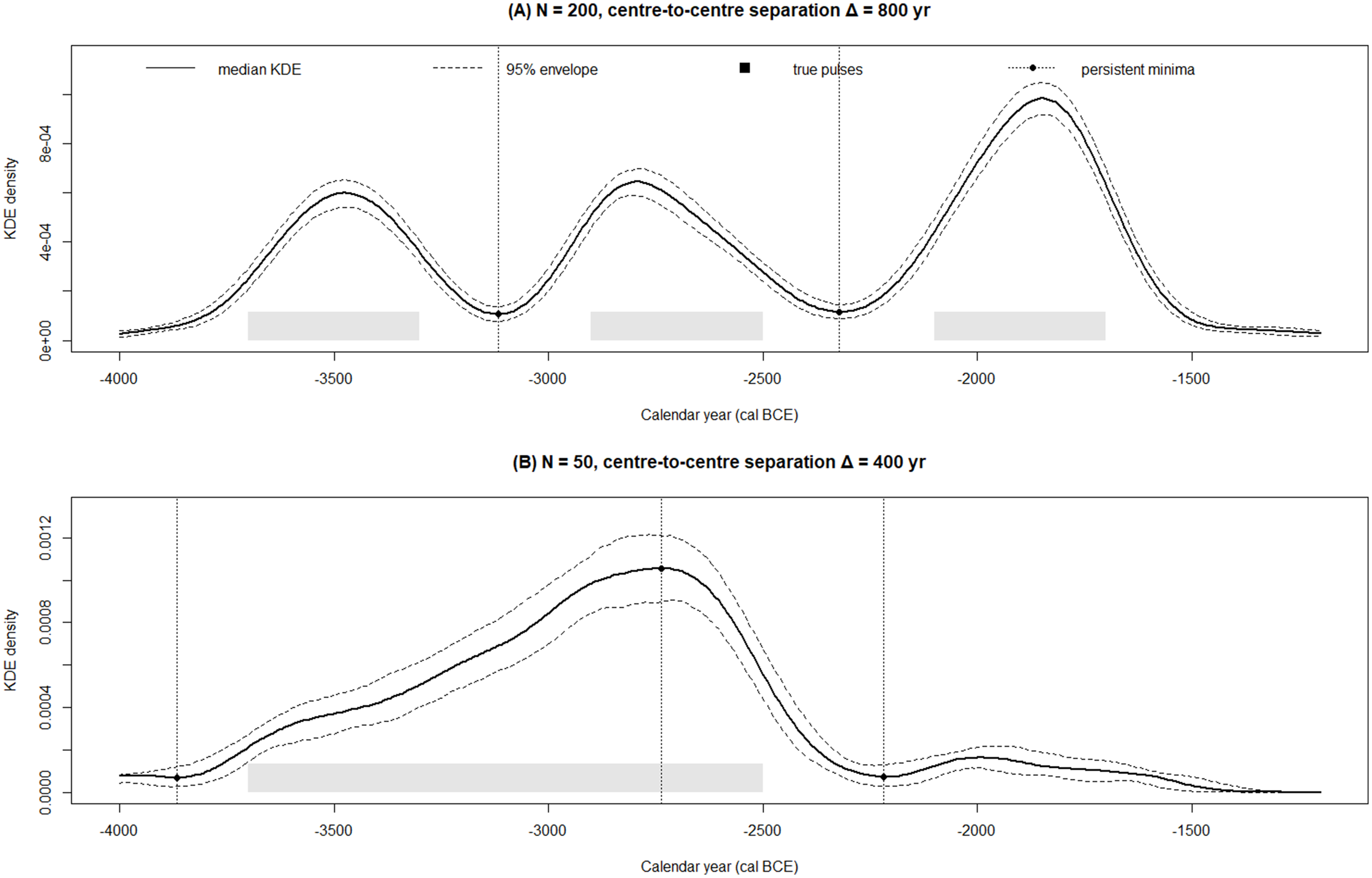
Two elements are key. First, radiocarbon dates are treated as calibrated posterior distributions rather than point estimates. A Monte Carlo ensemble of KDEs is generated by repeatedly sampling calendar ages from those posteriors (cf. Efron and Tibshirani Reference Efron and Tibshirani1994; Bronk Ramsey Reference Bronk Ramsey2017). Second, minima are accepted as pulse boundaries only when they appear in both the median KDE and the lower bound of a Monte Carlo envelope, so that shallow troughs likely to reflect sampling noise or calibration-induced shoulders are systematically excluded. The bandwidth and grid resolution explicitly control the scale at which pulses are defined (Silverman Reference Silverman2018; Scott Reference Scott2015; Sheather Reference Sheather2004). Figure 1 provides simple visual examples of the resulting segmentation for favourable and unfavourable cases.
Illustrative behaviour of the Monte Carlo KDE–minima algorithm under contrasting Level A conditions. (A) High-information case (N = 200, centre-to-centre separation Δ = 800 yr) showing recovery of the three-pulse structure. (B) Lower-information case (N = 50, Δ = 400 yr), where adjacent 400-year pulses abut and the inferred structure becomes less distinct. Solid line = median KDE; dashed lines = 95% Monte Carlo envelope; grey bars = true pulse intervals; dotted vertical lines and points = persistent minima retained as pulse boundaries. Together, the panels contrast a favourable case with wide separation and a more difficult case with fewer dates and limited separation.

Figure 1. Long description
Panel A: A line graph shows the high-information case with 200 samples and a center-to-center separation of 800 years. The x-axis represents calendar years in BCE, ranging from -4000 to -1500. The y-axis represents KDE density, ranging from 0 to 8e-04. The solid line indicates the median KDE, dashed lines represent the 95% Monte Carlo envelope, grey bars show true pulse intervals, and dotted vertical lines with points indicate persistent minima retained as pulse boundaries. The graph shows three distinct peaks corresponding to the true pulse intervals. Panel B: A line graph shows the lower-information case with 50 samples and a center-to-center separation of 400 years. The x-axis represents calendar years in BCE, ranging from -4000 to -1500. The y-axis represents KDE density, ranging from 0 to 0.0012. The solid line indicates the median KDE, dashed lines represent the 95% Monte Carlo envelope, grey bars show true pulse intervals, and dotted vertical lines with points indicate persistent minima retained as pulse boundaries. The graph shows a less distinct structure with a single prominent peak.
Substantively, the method is intended for descriptive segmentation of dated-event intensity, not for direct population estimation. It is most relevant when archaeologists are already reading broad phases visually from SPD or KDE curves and need a low-risk formalisation of that exploratory practice. When the research question instead requires posterior estimates of episode number, timing or intensity, explicit model-fitting approaches such as recent Poisson-process methods are preferable (Heaton et al. Reference Heaton, Al-assam and Bard2025; de Navascués et al. Reference de Navascués, Burgarella and Jakobsson2025).
The aim is therefore not to promote a universal demographic tool, but to map the conditions under which KDE–minima segmentation offers a defensible summary of a simple underlying process and the conditions under which it fails. Level A isolates smoothing and sampling in stylised calendar-time simulations. Level B adds laboratory error, calibration and method comparison under IntCal20, SHCal20 and a simple 50/50 mixed assignment. The mixed setup is used as a heterogeneity stress test rather than as a literal demographic scenario. A brief empirical illustration applies the procedure to a published radiocarbon corpus for the Kotosh Religious Tradition (KRT) in the Central Andes, where a Bayesian phase model already exists; this empirical application is discussed in detail in Section 3.3.
The results show that KDE–minima segmentation performs adequately only under relatively favourable conditions—well-separated pulses supported by large samples—and that calibration further reduces performance. The ensemble-based rule nonetheless offers a low-risk tactic for summarising broad episodes, with clearly defined limitations. The focus of the paper is thus on placing quantitative bounds on what KDE-based pulse detection can safely recover, rather than on promoting a new universal tool for demographic reconstruction (cf. Crema Reference Crema2022).
2 Methods
2.1 Activity pulses and Monte Carlo KDE–minima algorithm
Let
 $\{ {p_i}\left( t \right)\} _{i = 1}^n$
denote calibrated posterior distributions for
 $n$
radiocarbon determinations, where
 $t$
is calendar age. The goal is to partition the time axis into contiguous intervals within which the underlying event intensity can reasonably be treated as approximately homogeneous, and between which there is evidence for a lull in activity. These intervals are termed activity pulses. They are explicitly scale-dependent features of a smoothed intensity estimate at a chosen bandwidth
 $h$
and grid resolution, not direct estimates of a unique demographic trajectory (Silverman Reference Silverman2018; Scott Reference Scott2015).
The Monte Carlo KDE–minima procedure is:
-
1. For each replicate
 $r = 1, \ldots, R$
, draw a single calendar age
$t_i^{\left( r \right)}$
from each posterior
${p_i}\left( t \right)$
. Across replicates, these draws approximate integrating over the full posteriors (Efron and Tibshirani Reference Efron and Tibshirani1994; Bronk Ramsey Reference Bronk Ramsey2017).
-
2. For each replicate, construct a KDE
on a fixed calendar grid, where
${{\hat f}^{\left( r \right)}}\left( t \right) = {1 \over {nh}}\sum\limits_{i = 1}^n K \left( {{{t - t_i^{\left( r \right)}} \over h}} \right)$
$K$
is the standard normal density and
$h$
the bandwidth. The grid spacing is fine enough that minima can be located at a resolution of a few years relative to
$h$
(Silverman Reference Silverman2018; Scott Reference Scott2015).
-
3. At each grid point
${t_j}$
, compute the pointwise median
$\tilde f\left( {{t_j}} \right)$
and the 2.5–97.5% Monte Carlo envelope
$\left[ {{{\tilde f}_{0.025}}\left( {{t_j}} \right),{{\tilde f}_{0.975}}\left( {{t_j}} \right)} \right]$
over replicates. -
4. Identify local minima of
$\tilde f\left( t \right)$
and of the lower envelope
${\tilde f_{0.025}}\left( t \right)$
using the sign pattern of first differences along the grid. -
5. Mark a grid index
${j^{\rm{*}}}$
as a persistent minimum if it is a local minimum of the median KDE and there exists a minimum of the lower envelope within one grid step of
${j^{\rm{*}}}$
. -
6. Let accepted minima occur at calendar positions
${b_1}{\rm{ }} \lt \ldots{\rm{ }} \lt {b_{K - 1}}$
. Define
$K$
activity pulses as the intervals
$\left( { - \infty, {b_1}} \right],\left( {{b_1},{b_2}} \right], \ldots, \left( {{b_{K - 1}}, + \infty } \right)$
, truncated to the calendar range spanned by the data.


The requirement that minima be present in both the median and the lower envelope is intentionally conservative. A minimum visible in
 $\tilde f\left( t \right)$
but absent from
 ${\tilde f_{0.025}}\left( t \right)$
is treated as a likely artefact of sampling variability or calibration-induced shoulders. The single-grid-step neighbourhood allows for minor horizontal shifts in minima between the median and envelope. In spirit, the procedure is analogous to multi-scale curve exploration methods such as SiZer, which emphasise persistent structures over those that disappear under small perturbations (Chaudhuri and Marron Reference Chaudhuri and Marron1999). The examples in Figure 1 show how the algorithm behaves in an “easy” case with widely separated pulses and a “hard” case with fewer dates and substantially overlapping episodes.
In all simulations and empirical analyses, calendar grids are restricted to the window of interest, and pulses abutting the edges of this window must be interpreted cautiously because minima near boundaries are less stable. In practice, analysts should examine whether edge pulses persist when the analysis window is expanded or when
 $h$
is varied within a plausible range (Silverman Reference Silverman2018; Scott Reference Scott2015). The bandwidth range used throughout this study,
 $h = 80$
–120 yr, should be read as a decision-relevant multi-century smoothing regime rather than as an attempt to estimate an optimal bandwidth. The substantive target is the recovery of broad, multi-century pulses, not the finest-scale local structure visible in an SPD or KDE curve. Given the 400-year pulse widths used in the simulations, values in this range are large enough to suppress small shoulders and calibration-induced irregularities but still small enough not to force adjacent 400-year pulses to merge a priori. Formal bandwidth selectors exist (Sheather Reference Sheather2004; Silverman Reference Silverman2018; Scott Reference Scott2015), but for radiocarbon data with irregular calibration structure and posterior uncertainty, sensitivity over a plausible range is more informative than any single plug-in estimate. Bandwidth sensitivity for the KRT application is examined in the empirical illustration (Section 3.3).
2.2 Level A simulations: calendar-time pulses
Level A simulations operate directly in calendar time (BCE), isolating the effects of sample size, episode spacing and bandwidth without calibration. The underlying intensity
 $\lambda \left( t \right)$
is piecewise constant with three pulses and a uniform background. The configuration is summarised in Table 1. In the baseline design, three pulses of width 400 yr are centred at
 $ - 3500$
,
 $ - 2700$
and
 $ - 1900$
cal BCE, that is
 $\left[ {{s_1},{e_1}\left] = \right[ - 3700, - 3300\left] {,{\rm{\;\;}}} \right[{s_2},{e_2}\left] = \right[ - 2900, - 2500\left] {,{\rm{\;\;}}} \right[{s_3},{e_3}\left] = \right[ - 2100, - 1700} \right],$
with intensities
 ${\lambda _1} = 1$
,
 ${\lambda _2} = 1.5$
,
 ${\lambda _3} = 2$
and background intensity
 ${\lambda _{{\rm{bg}}}} = 0.1$
. The simulation window spans
 $ - 4000$
to
 $ - 1200$
cal BCE. Under these settings, the three pulses account for approximately 92% of expected events over the window. The low background component is included to prevent the simulations from collapsing into an unrealistically clean pulse-only system and to approximate the low-rate dated events that would often exist outside major activity clusters. This stylised, piecewise-constant configuration with equal-width pulses is not intended as a literal model of any particular archaeological sequence; it provides a controlled setting in which the joint effects of spacing, sample size and bandwidth on segmentation can be isolated.
Piecewise-constant intensity function for Level A simulations. For each pulse, the table lists the calendar-time start and end (cal BCE) and the event intensity
 ${\lambda _k}$
. A low background intensity
 ${\lambda _{{\rm{bg}}}} = 0.1$
applies across the intervals outside the pulses. Level B simulations use analogous 400-yr pulses in calendar years BP.

Table 1. Long description
A table with three rows and four columns. The columns are labeled Pulse ID, t_start (cal BCE), t_end (cal BCE), and λ_k. Row 1: Pulse ID 1, t_start -3700, t_end -3300, λ_k 1.0. Row 2: Pulse ID 2, t_start -2900, t_end -2500, λ_k 1.5. Row 3: Pulse ID 3, t_start -2100, t_end -1700, λ_k 2.0. The table lists the calendar-time start and end for each pulse and the event intensity λ_k. A low background intensity λ_bg = 0.1 applies across the intervals outside the pulses.
Throughout Level A, pulse width is fixed at 400 yr and separation
 ${\rm{\Delta }}$
is defined as the centre-to-centre distance between adjacent pulses. This distinction matters. When
 ${\rm{\Delta }} = 400$
yr, adjacent pulse edges abut; when
 $\Delta {\rm{ }} \lt 400$
yr, adjacent pulses overlap in calendar time; and when
 $\Delta {\rm{ }} \gt 400$
yr, a trough or lull exists between them. Reviewer concern about the recoverability of 400-year pulses at similar separations is therefore addressed here by making the relation between width and spacing explicit in both the design and the figure captions.
Events are generated by sampling segment membership with probability proportional to intensity
 $ \times $
duration and drawing times uniformly within segments. This yields true event times
 $\{ t_i^{{\rm{true}}}\} _{i = 1}^N$
. To mimic posterior uncertainty in calendar time without calibration, each event is perturbed by Gaussian error with
 $\sigma = 50$
yr, and the perturbed times are treated as posterior draws when constructing KDEs. Figure 1 illustrates the resulting KDEs and persistent minima for a well-separated case and a more challenging configuration.
KDEs are evaluated on a fixed grid of 400 equally spaced calendar points between
 $ - 4000$
and
 $ - 1200$
cal BCE. The main design varies the total sample size
 $N \in \left\{ {50,100,200,500} \right\}$
, the centre-to-centre separation between pulses
 ${\rm{\Delta }} \in \left\{ {200,400,600,800} \right\}$
yr, and the bandwidth
 $h \in \left\{ {80,100,120} \right\}$
yr. For each combination of
 $\left( {N,{\rm{\Delta }},h} \right)$
, 200 datasets are simulated and analysed with the ensemble KDE–minima rule and with a naive single-KDE minima rule that uses minima of a single KDE constructed from a single draw of calendar ages. The bandwidth values are chosen to interrogate the same multi-century regime across all simulations: they are not intended as optimal selectors, but as a plausible decision range for asking whether 400-year pulses separated by several centuries remain recoverable after smoothing. In other words, the goal is conservative segmentation at the scale of broad episodes, not local feature recovery at the finest temporal resolution. Values substantially larger than 120 yr would increasingly force adjacent episodes to merge, whereas substantially smaller values would make spurious local minima more common. The chosen range therefore brackets a practical compromise between resolution and stability while keeping the design tractable (Bronk Ramsey Reference Bronk Ramsey2017; Crema and Bevan Reference Crema and Bevan2021; Silverman Reference Silverman2018; Scott Reference Scott2015; Sheather Reference Sheather2004).
2.3 Level B simulations: calibrated dates and alternative segmentation methods
Level B simulations extend Level A by including radiocarbon measurement error and calibration, and by comparing the ensemble rule with two alternatives: the naive single-KDE minima rule and a Poisson changepoint model fitted to binned counts.
The simulation window spans 2000–5000 cal BP. Three pulses of width 400 yr are centred at 4500, 3500 and 2500 cal BP, with equal intensities and a background intensity
 ${\lambda _{{\rm{bg}}}} = 0.1$
, so that pulses contribute approximately 87% of expected events. As in Level A, the low background component prevents the simulations from collapsing into an unrealistically clean pulse-only system and approximates the low-rate dated events expected outside major activity clusters. All pulses have the same height in Level B to focus on calibration effects; the structure is analogous to Table 1 but expressed in calendar years BP. As with Level A, this is a deliberately simplified configuration: real sequences will show unequal pulse heights, variable widths and superimposed long-term trends, so the performance estimates reported here should be read as benchmarks under idealised conditions rather than as universal expectations.
For each true event time
 $t_i^{{\rm{true}}}$
, an expected radiocarbon age
 ${\mu _i}$
is first obtained from a specified calibration curve by uncalibration. Three calibration setups are considered:
-
1. Pure IntCal20 (Reimer et al. Reference Reimer, Austin, Bard, Bayliss, Blackwell, Bronk Ramsey, Butzin, Cheng, Edwards and Friedrich2020),
-
2. Pure SHCal20 (Hogg et al. Reference Hogg, Heaton, Hua, Palmer, Turney, Southon, Bayliss, Blackwell, Boswijk and Bronk Ramsey2020),
-
3. A simple “mixed” configuration in which each event is randomly assigned to IntCal20 or SHCal20 with equal probability.
These three setups are included not because large curve-specific differences are expected a priori, but to test whether the broad conclusions of the method are robust to reasonable hemispheric calibration structure. The mixed configuration is therefore a simple heterogeneity stress test rather than a literal demographic scenario.
In all cases, a laboratory measurement
 ${A_i}$
is then simulated from a normal distribution with mean
 ${\mu _i}$
and standard deviation
 ${\sigma _A} = 30$
 ${{\rm{\;}}^{14}}$
C yr. These simulated radiocarbon ages and their associated errors are recalibrated using the same curve assignment that generated
 ${\mu _i}$
, yielding posterior discrete distributions for each date. The KDE ensemble is then constructed as in Section 2.1, using
 $R = 300$
posterior draws and a fixed grid of 400 calendar points between 2000 and 5000 cal BP. The simulation pipeline is therefore: true calendar ages
 $ \to $
expected radiocarbon ages under a chosen curve
 $ \to $
laboratory error
 $ \to $
recalibration
 $ \to $
Monte Carlo KDE ensemble.
The Level B design varies
 $N \in \left\{ {50,100,200,500} \right\}$
,
 $h \in \left\{ {80,100,120} \right\}$
yr and calibration setup, and performs 200 replicates per combination, per segmentation method (ensemble rule, naive KDE, Poisson changepoint). The Poisson model operates on counts in 50-yr bins and assumes a piecewise-constant intensity; the number and locations of changepoints are estimated with the PELT multiple-changepoint algorithm in the changepoint package (cpt.meanvar, test.stat = “Poisson”) using a Schwarz information criterion (SIC, i.e. BIC) penalty on the log-likelihood (Heaton et al. Reference Heaton, Al-assam and Bard2025; de Navascués et al. Reference de Navascués, Burgarella and Jakobsson2025).
2.4 Performance metrics
For both simulation levels, performance is evaluated by comparing the inferred number of pulses
 $\hat K$
and their boundaries with the true configuration:
-
Pulse-count accuracy. For each replicate,
$\hat K$
is compared to the true
${K_{{\rm{true}}}} = 3$
. Results are summarised by the probabilities of correct recovery (
${p_{{\rm{correct}}}}$
), under-segmentation (
${p_{{\rm{under}}}}$
,
$\hat K{\rm{ }} \lt {K_{{\rm{true}}}}$
) and over-segmentation (
${p_{{\rm{over}}}}$
,
$\hat K{\rm{ }} \gt {K_{{\rm{true}}}}$
). -
Boundary error. Boundary accuracy is summarised in two ways. First, for all replicates, an unconditional mean absolute boundary error (yr) is computed using nearest-boundary matching. This metric remains useful descriptively but becomes difficult to compare across methods when they differ strongly in their tendency to over-segment. Second, for replicates with
$\hat K = {K_{{\rm{true}}}}$
, a conditional mean absolute boundary error is computed by ordered one-to-one pairing of sorted estimated and true boundaries. This conditional metric provides the cleaner comparison of temporal localisation once the correct pulse count has been recovered. For replicates with
$\hat K \ne {K_{{\rm{true}}}}$
, supplementary tables also report the unconditional error for incorrect-
$K$
cases.


These metrics separate recovery of the overall pulse structure from temporal localisation once that structure has been obtained. This dual perspective mirrors recent simulation-based evaluations of radiocarbon-frequency methods and avoids treating boundary precision as commensurate across methods with different segmentation tendencies (Contreras and Meadows Reference Contreras and Meadows2014; Bevan and Crema Reference Bevan and Crema2021; Crema Reference Crema2022). A compact synthesis across information regimes is provided in Table 2, while detailed simulation values appear in Supplementary Tables S1–S3.
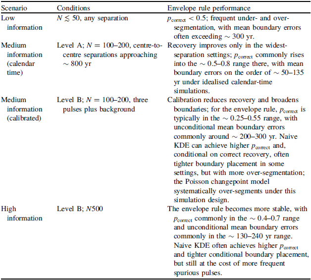
Condensed qualitative summary of envelope KDE–minima performance across simulation regimes. Statements are approximate syntheses derived from Supplementary Tables S1–S3 for bandwidths 80–120 yr.

Table 2. Long description
A table comparing envelope rule performance across different scenarios and conditions. The table has three columns: Scenario, Conditions, and Envelope rule performance. It contains four rows with different scenarios: Low information, Medium information (calendar time), Medium information (calibrated), and High information. Each row details the conditions and the corresponding envelope rule performance. For example, under Low information with N less than or equal to 50 and any separation, the performance is frequent under- and over-segmentation with mean boundary errors often exceeding 300 years. Under Medium information (calendar time) with N between 100 and 200 and centre-to-centre separations approaching 800 years, recovery improves in the widest-separation settings with p_correct commonly rising into the 0.5-0.8 range and mean boundary errors around 50-135 years. Under Medium information (calibrated) with N between 100 and 200 and three pulses plus background, calibration reduces recovery and broadens boundaries with p_correct typically in the 0.25-0.55 range and mean boundary errors around 200-300 years. Under High information with N 500, the envelope rule becomes more stable with p_correct commonly in the 0.4-0.7 range and mean boundary errors around 130-240 years.
3 Results
3.1 Level A: calendar-time pulses
Level A simulations confirm that segmentation performance is governed primarily by episode spacing, sample size and bandwidth. When pulses are strongly overlapping (
 ${\rm{\Delta }} = 200$
or 400 yr, with fixed pulse width = 400 yr), all methods struggle:
 ${p_{{\rm{correct}}}}$
remains low and both under- and over-segmentation are common, even at
 $N = 500$
. Under these conditions, the smooth intensity itself contains limited information about distinct episodes.
For well-separated pulses (
 ${\rm{\Delta }} \approx 800$
yr), performance improves markedly. With
 $N \geqslant 200$
and moderate bandwidths (
 $h = 80$
–120 yr), the ensemble rule recovers the correct three-pulse structure in a majority of replicates, and boundary errors are typically on the order of one to two bandwidths (Figure 1). However, the method remains conservative: at small and moderate sample sizes (
 $N = 50$
–100), under-segmentation is more common than over-segmentation, and pulses tend to be temporally diffuse.
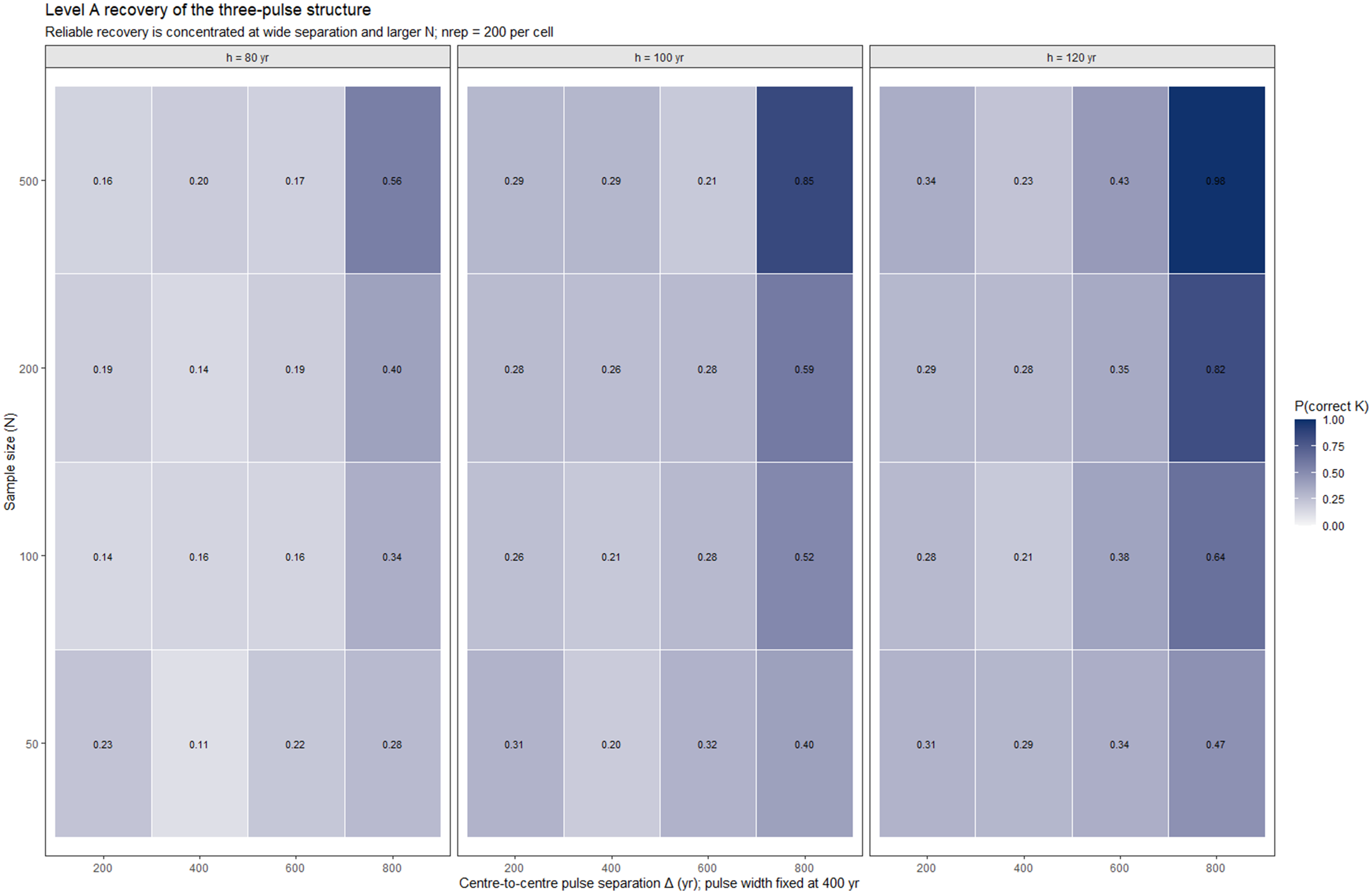
Figure 2 summarises
 ${p_{{\rm{correct}}}}$
for the envelope-based rule as a function of
 $N$
, centre-to-centre separation
 ${\rm{\Delta }}$
, and
 $h$
. High values of
 ${p_{{\rm{correct}}}}$
are confined to cells with both large
 $N$
and wide separation (bottom-right corner of each panel), reinforcing the conclusion that KDE–minima segmentation is reliable only under favourable conditions. Table 2 condenses these patterns into four qualitative regimes (low, medium calendar-time, medium calibrated and high information), with approximate ranges for
 ${p_{{\rm{correct}}}}$
and boundary error.
Level A recovery of the three-pulse structure under the envelope KDE–minima rule. Heatmaps show the probability of correct pulse-count recovery, P(K-hat = K-true), across sample size (N = 50, 100, 200, 500), centre-to-centre pulse separation (Δ = 200, 400, 600, 800 yr), and bandwidth (h = 80, 100, 120 yr). Pulse width is fixed at 400 yr. Reliable recovery is concentrated in the widest-separation settings and improves with larger sample size, showing that recoverability depends jointly on spacing, information content, and smoothing scale. Each cell summarises 200 Monte Carlo replicates.

Figure 2. Long description
Panel A: A heat map showing the probability of correct pulse-count recovery with a bandwidth of 80 years. The x-axis represents centre-to-centre pulse separation in years (200, 400, 600, 800), and the y-axis represents sample size (50, 100, 200, 500). The color scale indicates the probability of correct recovery, with darker colors representing higher probabilities. Notable values include 0.56 at the highest separation and sample size. Panel B: A heat map with a bandwidth of 100 years. The axes and color scale are the same as in Panel A. Notable values include 0.85 at the highest separation and sample size. Panel C: A heat map with a bandwidth of 120 years. The axes and color scale are the same as in the previous panels. Notable values include 0.98 at the highest separation and sample size.
Compared to the naive single-KDE minima rule, the ensemble rule substantially reduces over-segmentation. The naive rule tends to interpret shallow shoulders and local irregularities as separate pulses, especially at smaller
 $N$
and smaller
 $h$
, yielding high
 ${p_{{\rm{over}}}}$
. The ensemble rule discards many of these minima because they are not stable in the lower envelope, trading a modest loss of sensitivity for greater robustness against spurious episodes. This behaviour is consistent with general insights from multi-scale curve exploration, where persistent features are privileged over local noise (Chaudhuri and Marron Reference Chaudhuri and Marron1999). Supplementary Table S1 and Supplementary Figure S02 give full numerical and graphical comparisons for the Level A scenarios. Curve-specific Level B KDE results are reported in Supplementary Table S03 and Supplementary Figure S03.
3.2 Level B: calibrated dates and segmentation methods
Level B simulations show that calibration further degrades segmentation performance. For a given combination of
 $N$
,
 $h$
and curve assignment,
 ${p_{{\rm{correct}}}}$
is generally lower than in Level A, and boundary errors increase. This reflects the additional smoothing and distortion introduced by the calibration curve and measurement error, as well as the non-linear relationship between true calendar time and radiocarbon age (Reimer et al. Reference Reimer, Austin, Bard, Bayliss, Blackwell, Bronk Ramsey, Butzin, Cheng, Edwards and Friedrich2020; Hogg et al. Reference Hogg, Heaton, Hua, Palmer, Turney, Southon, Bayliss, Blackwell, Boswijk and Bronk Ramsey2020; Bronk Ramsey Reference Bronk Ramsey2017).
Differences between calibration setups (IntCal20, SHCal20, mixed) are consistently small relative to the effects of sample size, bandwidth and segmentation rule. This is a negative but informative result, because the three curve setups were included precisely to test whether the broad conclusions are robust to reasonable hemispheric calibration structure. At the multi-century scale considered here, the mixed configuration behaves similarly to the pure curves, suggesting that curve choice is second-order relative to the basic information content of the sample.
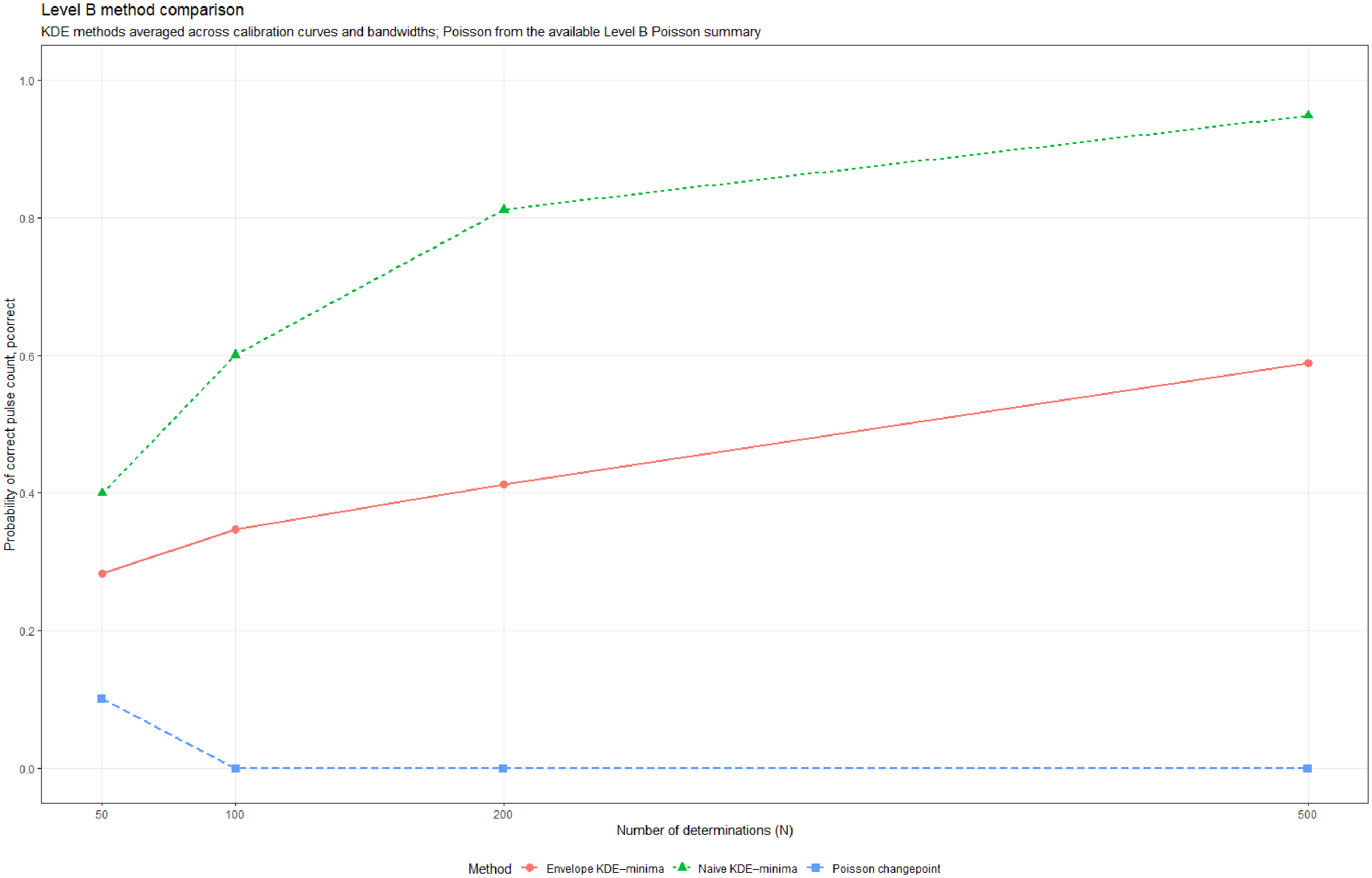
Figure 3 compares
 ${p_{{\rm{correct}}}}$
for the three segmentation methods as a function of
 $N$
, averaging over bandwidths and calibration setups. It should therefore be read as a collapsed method-comparison synthesis rather than as a substitute for the curve- and bandwidth-stratified supplementary outputs. Curve-specific Level B KDE results are shown in Supplementary Table S3 and the corresponding supplementary figure. Within this synthesis, both KDE-based methods improve with increasing
 $N$
, but they differ in trade-off structure: the envelope rule is more conservative and suppresses many spurious minima, whereas the naive KDE rule can attain higher
 ${p_{{\rm{correct}}}}$
at the cost of more frequent over-segmentation. The Poisson changepoint model performs poorly under the present design. In the curve-specific Poisson outputs,
 ${p_{{\rm{correct}}}}$
is low at
 $N = 50$
and falls to zero at
 $N = 100$
, 200 and 500 across all three calibration setups, while
 ${p_{{\rm{over}}}}$
is systematically high. The Poisson model is therefore included here as a contrasting model-fitting benchmark rather than as a superior segmentation solution.
Collapsed Level B comparison of segmentation methods after averaging KDE results across calibration curves and bandwidths. The plot shows the probability of correct pulse-count recovery for the envelope KDE–minima rule, the naive single-KDE minima rule, and the Poisson changepoint model as a function of sample size. It is intended as a summary of method trade-offs rather than a substitute for the curve- and bandwidth-stratified supplementary results: naive KDE achieves higher recovery but with greater risk of over-segmentation, the envelope rule is more conservative, and the Poisson changepoint model over segments systematically under the present calibrated design.

Because methods differ sharply in their tendency to over-segment, unconditional boundary error alone is not sufficient for comparing temporal localisation. Supplementary Table S3 therefore also reports boundary error conditional on correct pulse-count recovery. Under this stricter comparison, the naive KDE rule typically yields tighter boundary placement than the envelope rule, whereas the main advantage of the envelope rule lies in its more conservative segmentation and lower susceptibility to unstable minima.
Overall, high probabilities of recovering the true three-pulse structure are achieved only under favourable conditions: widely separated episodes and substantial sample sizes. Even then, boundary estimates remain uncertain at the scale of several tens to a few hundred years. The main practical contrast is therefore not between higher sensitivity and higher precision, but between a conservative envelope rule that limits spurious splitting and a more aggressive naive rule that often localises boundaries more tightly when correct, but at a substantially higher risk of extra pulses.
3.3 Empirical illustration: Kotosh Religious Tradition
To illustrate the method on real data, the ensemble KDE–minima procedure is applied to a published radiocarbon corpus for the Kotosh Religious Tradition (KRT) in the Central Andes. That dataset comprises 170 determinations from 16 Late Archaic and Formative ceremonial sites, modelled in OxCal as a three-episode regional sequence with two nested subtraditions (Mito Tradition and Kotosh Broad Tradition) (Mesia-Montenegro Reference Mesia-Montenegro2025). The present analysis does not introduce new chronological modelling; it uses posterior calendar-age samples from the published OxCal model as input to the KDE–minima algorithm, treating the Bayesian model as a benchmark.
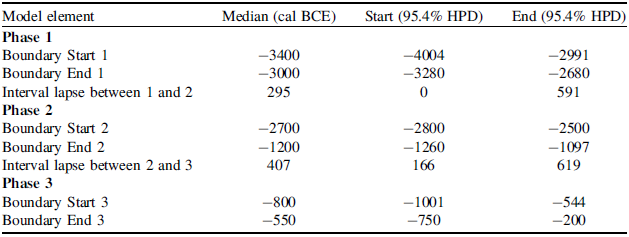
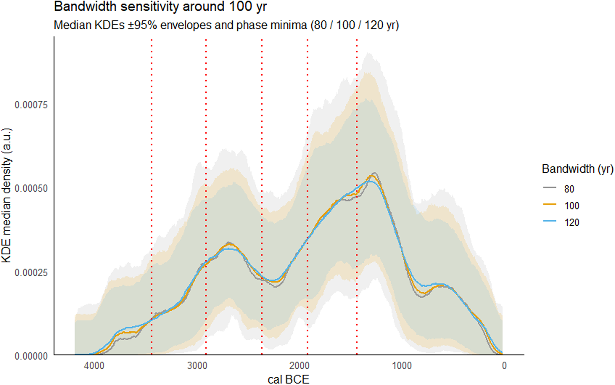
Table 3 summarises the three Bayesian KRT episodes, reporting median boundary ages and 95.4% highest posterior density (HPD) intervals. Posterior samples for all KRT events are pooled and analysed with bandwidths of 80, 100 and 120 yr and a 95.4% envelope. For each bandwidth, the ensemble KDE and persistent minima are computed, and the resulting pulses are compared qualitatively with the three Bayesian regional episodes. Figure 4 summarises this bandwidth sensitivity: the main three-episode structure is robust across bandwidths, but the exact locations of minima and the sharpness of intervening troughs vary. In particular, edge pulses and minor shoulders are more unstable than the central episode, consistent with the simulation results.
Modelled boundaries, medians and 95.4% highest posterior density (HPD) intervals for the three Bayesian episodes of the Kotosh Religious Tradition (KRT) regional sequence. Times are in cal BCE. These values are taken from the OxCal phase model reported in Mesia-Montenegro (Reference Mesia-Montenegro2025) and provide the Bayesian frame of reference for the KDE–minima pulses shown in Figure 4.

Table 3. Long description
A table summarizing Bayesian KRT episodes with median boundary ages and 95.4% HPD intervals. The table has 10 rows and 4 columns. The columns are labeled ‘Model element’, ‘Median (cal BCE)’, ‘Start (95.4% HPD)’, and ‘End (95.4% HPD)’. The rows are grouped into three phases. Phase 1 includes Boundary Start 1, Boundary End 1, and Interval lapse between 1 and 2. Phase 2 includes Boundary Start 2, Boundary End 2, and Interval lapse between 2 and 3. Phase 3 includes Boundary Start 3 and Boundary End 3. Each row lists the median age and the start and end of the 95.4% HPD interval for each boundary or interval.
Bandwidth sensitivity of the Kotosh Religious Tradition illustration. Median KDEs and 95.4% envelopes are shown for bandwidths h = 80, 100, and 120 yr, with vertical dotted lines marking minima identified across the examined bandwidths. The principal multi-episode structure is broadly stable across this range, whereas the exact positions of minima, the sharpness of intervening troughs, and edge or shoulder features remain bandwidth-sensitive. The figure is therefore intended to show robustness of the broad pattern together with uncertainty in finer segmentation details.

The KRT example is therefore best read as a demonstration of behaviour on a large, archaeologically structured dataset with a known Bayesian benchmark. It highlights both the utility and the limits of the method: the ensemble rule can summarise broad episodes in a manner broadly consistent with a more complex phase model, but it cannot substitute for explicit modelling when precise boundaries or site-level differences are required (Crema Reference Crema2022; Mesia-Montenegro Reference Mesia-Montenegro2025). A brief SiZer-based sensitivity check is included in the supplementary material as an additional multi-scale diagnostic rather than as an alternative phase estimate. Under the stricter operational rule adopted in the revised analysis, no stable SiZer episodes were identified for the high-information Level A scenario, reinforcing the scale dependence of exploratory segmentation.
4 Discussion
4.1 Positioning within radiocarbon-frequency methods
The KDE–minima procedure is best understood as a descriptive segmentation of dated-event intensity within the reconstructive family of radiocarbon-frequency approaches. It does not estimate population size directly and is not designed to yield posterior statements about episode number, timing or magnitude. Its practical niche is narrower: to formalise the common archaeological practice of visually reading broad phases from SPD or KDE curves while making the smoothing dependence explicit and limiting spurious minima (Crema and Bevan Reference Crema and Bevan2021; Crema Reference Crema2022). In that sense it complements, rather than competes with, hypothesis-testing approaches and explicit model-fitting frameworks. When the substantive target is posterior inference on rates, changepoints or episode intensity, Poisson- or Cox-process models remain preferable (Heaton et al. Reference Heaton, Al-assam and Bard2025; de Navascués et al. Reference de Navascués, Burgarella and Jakobsson2025).
4.2 Practical guidance and limitations
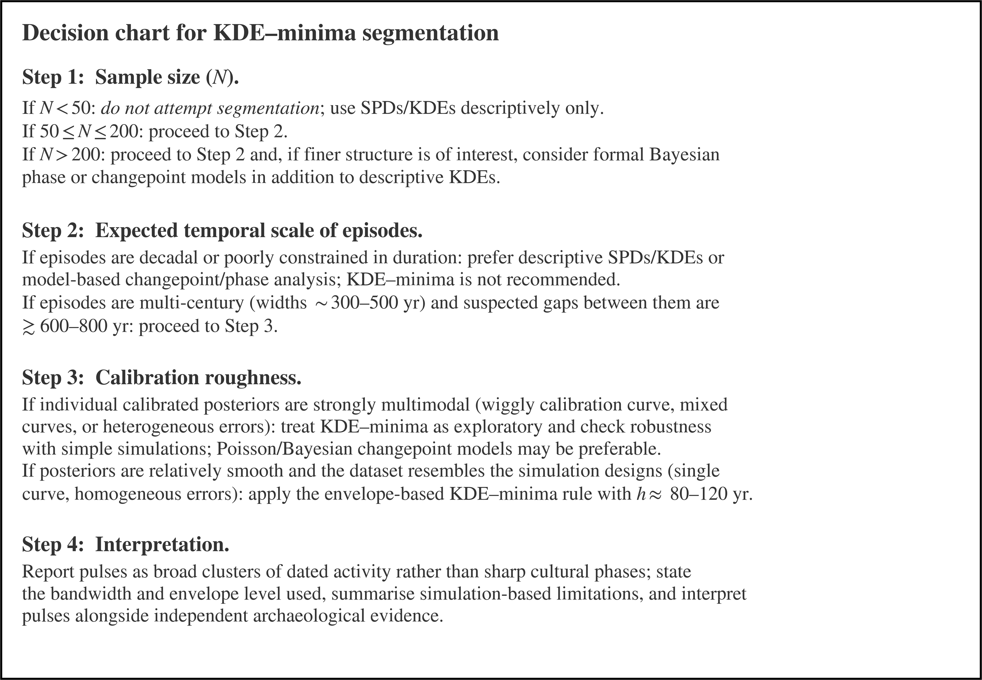
The simulations make clear that KDE–minima pulses should be interpreted cautiously. Figure 5 provides a decision chart that synthesises the main lessons; key points are:
-
Sample size and separation. Reliable recovery of episode counts and approximate boundaries occurs only when pulses are separated by several bandwidths (here
$ \approx 800$
yr, with pulse width fixed at 400 yr) and when each episode is supported by on the order of 100 or more determinations. At smaller
$N$
or with closely spaced pulses, under- and over-segmentation are common, consistent with earlier warnings about the limits of demographic inference from sparse radiocarbon series (Contreras and Meadows Reference Contreras and Meadows2014; Crema Reference Crema2022). This regime-based view is summarised in Table 2. -
Bandwidth choice. The bandwidth
$h$
controls the scale at which pulses are visible. Here
$h = 80$
–120 yr is used as a decision-relevant multi-century range, not as an estimate of an optimal smoothing parameter. The objective is conservative segmentation of broad episodes a few hundred years wide, not recovery of the finest local features in an SPD or KDE curve. Researchers should therefore inspect whether
$\hat K$
and boundary locations remain stable across a plausible range of
$h$
rather than privilege a single value (Silverman Reference Silverman2018; Scott Reference Scott2015; Sheather Reference Sheather2004; Crema Reference Crema2022). The KRT example (Figure 4) illustrates both robust features and bandwidth-sensitive details. -
Calibration effects. Calibration-curve structure and measurement error further blur episodes and can introduce spurious features. The three Level B curve setups were included to test robustness to reasonable hemispheric calibration structure, not because large differences were expected a priori. Their similarity is therefore informative: at the multi-century scales examined here, curve choice is second-order relative to sample size, bandwidth and segmentation rule. The mixed configuration should be read as a heterogeneity stress test rather than as a literal demographic scenario (Reimer et al. Reference Reimer, Austin, Bard, Bayliss, Blackwell, Bronk Ramsey, Butzin, Cheng, Edwards and Friedrich2020; Hogg et al. Reference Hogg, Heaton, Hua, Palmer, Turney, Southon, Bayliss, Blackwell, Boswijk and Bronk Ramsey2020; Crema and Bevan Reference Crema and Bevan2021).
-
Method trade-offs. Under the present calibrated design, the naive KDE rule often attains higher pulse-count recovery and, conditional on correct recovery, typically tighter boundary localisation than the envelope rule. Its cost is a markedly higher tendency to over-segment. The envelope rule’s main advantage is therefore not sharper timing but lower-risk segmentation through the suppression of unstable minima. The Poisson changepoint model, in contrast, systematically over-segments and does not provide a competitive summary for these simulated data. Figure 3 should therefore be read as a synthesis of these trade-offs rather than as a universal ranking.
-
Uncertainty. The method as implemented here provides no direct probabilistic measure of uncertainty in
$K$
or in boundary locations for empirical data. A natural extension would be to summarise the distribution of
$\hat K$
and of minima positions across Monte Carlo replicates and across bandwidths, thereby providing informal credibility intervals for pulses (cf. Efron and Tibshirani Reference Efron and Tibshirani1994; Chaudhuri and Marron Reference Chaudhuri and Marron1999).


Heuristic decision chart for KDE–minima segmentation of radiocarbon sequences. The chart summarises the main lessons of the simulation study: segmentation is most defensible for broad multi century episodes, sufficiently large samples, and relatively smooth calibrated posteriors; calibration roughness, small sample sizes, and closely spaced episodes increase the risks of under- and over segmentation. The chart should be read as a practical guide derived from the simulation designs examined here, not as a universal thresholding rule for all archaeological radiocarbon datasets.

The method is therefore best viewed as a low-risk, exploratory tool for summarising broad episodes in well-sampled sequences, not as a general solution to the phase-identification problem. For many research questions, especially those requiring precise phase boundaries or strong causal inference, explicit Bayesian or likelihood-based event-count models remain preferable (Crema and Bevan Reference Crema and Bevan2021; Heaton et al. Reference Heaton, Al-assam and Bard2025; de Navascués et al. Reference de Navascués, Burgarella and Jakobsson2025).
4.3 Future directions
Several extensions remain necessary. The simulations used equal-width pulses and, in Level B, equal heights; heterogeneous pulse shapes, overlapping shoulders and superimposed long-term trends are common in real data and will likely reduce performance further. Non-stationary sampling intensity and taphonomic loss were not explicitly modelled, and integrating plausible sampling processes would sharpen guidance on minimal data requirements and likely biases (Surovell et al. Reference Surovell, Finley, Smith, Brantingham and Kelly2009; Bevan and Crema Reference Bevan and Crema2021; Crema Reference Crema2022). Empirical uncertainty summaries for
 $\hat K$
and boundary positions, and closer integration with recent Poisson-process event-count models, remain the most useful next steps (Heaton et al. Reference Heaton, Al-assam and Bard2025; de Navascués et al. Reference de Navascués, Burgarella and Jakobsson2025).
5 Conclusions
The Monte Carlo KDE–minima procedure can recover broad activity pulses only under restricted conditions: episodes must be widely separated relative to their width, sample sizes must be on the order of at least 100–200 dates, and the resulting segmentation must remain stable across a defensible bandwidth range. Under poorer information conditions, especially after calibration, the method readily merges episodes or produces temporally diffuse boundaries. It should therefore be used for descriptive segmentation of dated-event intensity, not as a direct estimator of population history.
Within that restricted role, the envelope rule offers a conservative, low-risk summary because it suppresses unstable minima. Its advantage is not sharper boundary localisation: conditional on correct recovery, naive KDE typically places boundaries more tightly, but it does so alongside a much higher tendency to over-segment. At the multi-century scale examined here, differences among IntCal20, SHCal20 and the mixed calibration setup are small, so curve choice is secondary to sample size, bandwidth and segmentation rule.
A practical decision rule follows. Use KDE–minima segmentation only when the question concerns broad episodes, the dated sample is sufficiently large, and the segmentation is stable across a plausible bandwidth range. When the target is precise phase boundaries or posterior inference on episode number, timing or intensity, explicit Bayesian or likelihood-based event-count models are preferable. The Kotosh Religious Tradition example shows that, under favourable conditions, the ensemble rule can provide a rapid summary consistent with a published Bayesian benchmark, but at coarser temporal resolution.
Supplementary material
To view supplementary material for this article, please visit https://doi.org/10.1017/RDC.2026.10258
Code and data availability
All R scripts, supplementary tables and figures are archived in an OSF open repository https://doi.org/10.17605/OSF.IO/JZ3PE, enabling reproduction and extension of the analyses. The repository includes R scripts for the Level A and Level B simulation experiments, functions implementing the Monte Carlo KDE–minima and naive segmentation rules, code for computing the performance metrics reported in the tables and figures, and scripts for fitting the Poisson changepoint model and running the SiZer comparison.
Acknowledgments
I would like to thank the reviewers for constructive comments on earlier versions of this work and the Universidad Privada del Norte for supporting this research.

 λk
 λbg=0.1


 Open access

