1. Introduction
Particle-laden turbulent flows are widely encountered in geophysical phenomena and industrial applications, such as sandstorm flow, pneumatic transport and spray combustion. Owing to the combined effects of particle inertia and turbulent mixing, inertial particles tend to exhibit a non-uniform distribution in space. This phenomenon is named inertial clustering or preferential concentration (Maxey Reference Maxey1987; Balachandar & Eaton Reference Balachandar and Eaton2010). It will significantly alter the spray combustion performance, pneumatic transport efficiency and plankton/pollutant dispersion. Furthermore, turbulent motions will also be affected in a feedback manner.
Particle clustering can be easily observed by flow visualization. One classic example is the aeolian streamer, which describes the strip-like concentration of wind-blown sand grains near the surface of a desert (Baas & Sherman Reference Baas and Sherman2005; Wang et al. Reference Wang, Feng, Zheng and Sung2019a). Several approaches, including the radial distribution function, the box-counting method and Voronoï analysis, have been devised for rigorous detection and quantification of particle clusters. The last approach, i.e. Voronoï analysis, was first introduced to the two-phase flow community by Monchaux, Bourgoin & Cartellier (Reference Monchaux, Bourgoin and Cartellier2010). This method measures local particle concentration by areas of Voronoï cells of discrete particles, whose probability distribution function (p.d.f.) is compared with a random Poisson distribution to differentiate particle clusters from particle voids. Unlike the box-counting method (Aliseda et al. Reference Aliseda, Cartellier, Hainaux and Lasheras2002), no subjective detection threshold is needed. This feature makes it a popular tool in the study of particle clustering in homogenous isotropic turbulence (HIT) (Tagawa et al. Reference Tagawa, Mercado, Prakash, Calzavarini, Sun and Lohse2012; Obligado et al. Reference Obligado, Teitelbaum, Cartellier, Mininni and Bourgoin2014; Baker et al. Reference Baker, Frankel, Mani and Coletti2017; Sumbekova et al. Reference Sumbekova, Cartellier, Aliseda and Bourgoin2017) and turbulent channel flows (TCFs) (Rabencov & van Hout Reference Rabencov and van Hout2015; Yuan et al. Reference Yuan, Zhao, Andersson and Deng2018).
The particle clustering involved in particle–turbulence interaction is a complex process, since it presents multiscale kinematics and dynamics that are determined or affected by various controlling parameters. Various mechanisms responsible for particle clustering, especially in homogeneous turbulence, have been proposed in the past. Among them, the centrifuging mechanism, also known as the strain/vorticity selection mechanism, might be the earliest one being identified in HIT (Maxey Reference Maxey1987; Tagawa et al. Reference Tagawa, Mercado, Prakash, Calzavarini, Sun and Lohse2012; Baker et al. Reference Baker, Frankel, Mani and Coletti2017). According to this mechanism, heavy particles prefer to reside in the regions with high strain and low vorticity. The second one is the so-called sweep–stick mechanism, which attributes the clustering of inertial particles to the clustering of acceleration stagnation points in the fluid flow (Goto & Vassilicos Reference Goto and Vassilicos2008; Coleman & Vassilicos Reference Coleman and Vassilicos2009). Bragg, Ireland & Collins (Reference Bragg, Ireland and Collins2015a) later found that the preferential sampling of the coarse-grained velocity gradient tensor in the fluid phase leads to particle clustering when  $St_r\ll$ 1 (
 $St_r$ is the Stokes number based on the eddy turnover time at separation
 $r$), while a path history symmetry-breaking mechanism (Zaichik & Alipchenkov Reference Zaichik and Alipchenkov2009) contributes to particle clustering for
 $St_r\geq 1$. Although these mechanisms focus on different flow-field quantities for a cause-and-effect explanation, the manifestation that inertial particles accumulate in high-strain and low-rotation regions has not been disputed (Bragg, Ireland & Collins Reference Bragg, Ireland and Collins2015b). On the other hand, for wall-bounded turbulence, the wall-normal inhomogeneity of the mean shear, the wall blockage effect and the wide spectrum of turbulent structures complicate the picture of preferential particle concentration. Turbophoresis, which suggests that particles prefer to accumulate towards regions with low turbulent fluctuation, is the most commonly invoked mechanism in this case (Soldati & Marchioli Reference Soldati and Marchioli2009; Nowbahar et al. Reference Nowbahar, Sardina, Picano and Brandt2013). It is believed to account for the formation of particle streaks in the near-wall region that are in tight spatial correlation with fluid-phase low-speed streaks (Yang, Zhao & Andersson Reference Yang, Zhao and Andersson2017a; Lee & Lee Reference Lee and Lee2019; Liu et al. Reference Liu, Jiang, Lee and Hu2020).
The effect of particle clustering on the kinematics of both turbulence and particles is another interesting issue. Owing to the comparatively higher particle concentration, the degree of particle–turbulence interaction inside clusters can be significantly altered (Elghobashi Reference Elghobashi1994). This phenomenon has been found to result in significant consequences in both HIT and wall-bounded turbulence, including the enhancement of turbulence modification (Eaton & Fessler Reference Eaton and Fessler1994) and the increase of local inter-particle collision rate (Ernst, Sommerfeld & Laín Reference Ernst, Sommerfeld and Laín2019). Furthermore, in both HIT and vertical TCF, the gravitational settling of inertial particles in the regions of high particle concentration was found to be faster than that in low-concentration regions (Fong, Amili & Coletti Reference Fong, Amili and Coletti2019; Petersen, Baker & Coletti Reference Petersen, Baker and Coletti2019).
Despite these findings, there are several issues related to particle clustering that deserve to be further considered. First, fewer studies on particle clustering in wall-bounded turbulence, especially in a horizontally developed turbulent boundary layer (TBL) or atmospheric surface layer (ASL), where the free-stream flow is perpendicular to gravity, have been made. In the field of aeolian research, the state-of-the-art knowledge on the physics of wind-blown sand movements lacks a rigorous consensus on the role of particle clustering in affecting both sand grains’ local concentration and their vertical flux (Zheng Reference Zheng2009). This calls for a thorough characterization of the kinematics of particle clustering. Second, Monchaux et al. (Reference Monchaux, Bourgoin and Cartellier2010) have used Voronoï analysis to show the existence of self-similarity of the geometries of particle clusters in a particle-laden grid turbulence. It is now generally agreed that, in HIT, the self-similarity of particle clustering originates from the self-similarity of multiscale turbulent structures (Baker et al. Reference Baker, Frankel, Mani and Coletti2017; Sumbekova et al. Reference Sumbekova, Cartellier, Aliseda and Bourgoin2017). For two-phase wall-bounded turbulence, it is still unclear whether or not particle clustering presents geometric self-similarity; furthermore, statistical evidence for the spatial correlation between particle clusters and particular turbulent structures is still lacking.
With this background, the geometric and kinematic characteristics of particle clustering in a particle-laden TBL with large particle Stokes number, low particle volume fraction and moderate frictional Reynolds number were experimentally studied. This work is an extension of our previous study (Zhu et al. Reference Zhu, Pan, Wang, Liang and Ji2019). In that work, two-phase velocity fields in the streamwise–wall-normal plane of a spatially developing particle-laden TBL on a horizontal flat plate were measured by two-dimensional (2-D) particle image/tracking velocimetry (PIV/PTV). The effect of sand grains on turbulent modification, as well as the correlation between particle transport and turbulent structures, were studied in detail. Here, we mainly focus on the phenomenon of particle clustering and its relationship with self-similar turbulent structures via the techniques of 2-D Voronoï analysis, conditional statistics and spectral analysis.
Hereinafter, the two-phase flow fields, as well as the measurement details, are briefly reviewed in § 2. Voronoï analysis is performed in § 3 to show the presence of geometric self-similarity of particle clusters in the log layer of the TBL. A conceptual model to correlate particle clusters with wall-attached turbulent structures is presented in § 4, together with a series of statistical evidence in favour of it. The effect of particle clustering on the kinematics of both fluid phase and particle phase is discussed in § 5 via conditional statistics. Finally, additional discussions and concluding remarks are given in § 6.
2. Experimental set-up
The experiment set-up has been described in detail in Zhu et al. (Reference Zhu, Pan, Wang, Liang and Ji2019). Here, we only give a brief review to facilitate the following analysis. The tested TBL was spatially developed on the horizontal floor of a blow-type low-speed wind tunnel in Lanzhou University, PR China. The test section of this facility has a size of  $1.45\ \textrm {m} \times 1.3\ \textrm {m} \times 20\ \textrm {m}$ (height
 $\times$ width
 $\times$ length). The floor is composed of a glass pane and can be regarded as hydraulically smooth. In the experiment, the free-stream velocity was fixed at
 $U_\infty =7.5\ \textrm {m}\,\textrm {s} ^{-1}$ and the corresponding free-stream turbulence intensity was approximately
 $1\,\%$. The measurement station was at 8 m downstream of the transition tripping strip. The coordinate origin was set on the test floor, located at the inlet of the field of view (FOV) of the PIV/PTV measurement. Herein,
 $x$,
 $y$ and
 $z$ denote the streamwise, wall-normal and spanwise directions, respectively. Instantaneous and fluctuating velocity components along the three directions are
 $U,V,W$ and
 $u,v,w$. Inner scaling via friction velocity
 $u_\tau$ and wall unit
 $\nu /u_\tau$ is denoted as
 $(\cdot )^+$. The subscript
 $f$ or
 $p$ related to a variable denotes a quantity of fluid phase or particle phase, respectively.
For the particle-laden cases, sieved sand grains with a diameter of  $d_p=203\pm 89\ \mathrm {\mu }\textrm {m}$ and a mean density of
 $2600\ \textrm {kg}\,\textrm {m}^{-3}$ were evenly fed into the free stream through a well-controlled feeding system at the ceiling of the entrance of the test section. This forms a net sedimentation condition. Namely, sand grains descend downwards under the effect of gravity while convecting downstream driven by the flow. The streamwise gap from the sand-grain releasing station to the inlet of the PIV/PTV FOV was 8 m. Two bulk particle volume fractions, i.e.
 $\varPhi _1=7\times 10^{-5}$ and
 $11\times 10^{-5}$ , were tested. They are denoted as cases T1 and T2. Nominally, such bulk volume fractions fall in the two-way coupling regime (
 $10^{-6}<\varPhi _1< 10^{-3}$), which states that the feedback of particles on turbulent motion is evident but inter-particle collisions are negligible (Elghobashi Reference Elghobashi1994). Nevertheless, as will be shown later (in figure 2a), due to the net sedimentation condition, the local volume fraction varies by approximately two orders within the TBL. Such a strong vertical non-homogeneity disfavours a simplified classification of the particle–turbulence coupling regime. Therefore, the level of turbulence modification at different length scales, as well as at different flow regions of the TBL, will be scrutinized in the following.
The choice of releasing sand grains from the ceiling to form a net sedimentation condition is based on the consideration of keeping a steady smooth-wall condition. In contrast, a sand-bed faces a time-varied wall condition (Liu et al. Reference Liu, Jiang, Lee and Hu2020; Zheng, Wang & Zhu Reference Zheng, Wang and Zhu2021), which will inevitably alter the near-wall turbulent motions and thus bias the statistical and structural characteristics from a canonical TBL. In the present experiment, due to the dilute concentration and the relatively large friction velocity, there was no noticeable particle deposition on the floor.
In the 2-D PIV/PTV measurements, di-2-ethyl-hexyl-sebacate (DEHS) droplets with diameters of  $0.5 - 5 \ \mathrm {\mu }\textrm {m}$ were used as tracer particles of the fluid phase. The symmetric streamwise–wall-normal plane of the flow domain was illuminated by a laser sheet (with a thickness of
 $\Delta z\approx 1.0\ \textrm {mm}$) emitted from a double-pulsed Nd:YAG laser generator with a wavelength of 532 nm and an energy output of
 $200\ \textrm {mJ}\,\textrm {pulse}^{-1}$ through a set of shaping optical lenses. Four synchronized charge-coupled device (CCD) cameras (IMPERX ICL-B2520M), each with a resolution of
 $2456\ \textrm {pixel} \times 2058\ \textrm {pixel}$, were aligned along the streamwise direction to record the 2-D flow field at a sampling rate of 5 Hz. Such a multiple-camera configuration was designed to provide a large FOV, i.e.
 $\Delta X \times \Delta Y = 0.80\ \textrm {m} \times 0.16\ \textrm {m}$ or
 $2.67\delta \times 0.53\delta$, to resolve both small-scale fluctuations and large-scale motions (LSMs).
An in-house post-processing algorithm was used to calculate the velocity vectors of both tracer particles and individual sand grains from two-phase particle image pairs. The state-of-the-art algorithm for two-phase-flow measurement (Kiger & Pan Reference Kiger and Pan2000) was utilized. Namely, phase separation was conducted by a two-step size-based median filter, and velocity calculations were then performed by conventional PIV for the fluid phase and by cross-correlation-based PTV for the particle phase. In PIV, the final-pass interrogation window had a size of  $32\ \textrm {pixel} \times 32\ \textrm {pixel}$, corresponding to a spatial resolution of 68 wall units per vector. While in PTV, a cross-validation between forward and backward tracking was taken to minimize the effect of particle missing pairing. The velocity statistics of both phases were obtained from 9000 uncorrelated image pairs. Details of the PIV/PTV implementation, the zero-pressure-gradient condition and the calibration of the baseline flow (case S) can be found in Zhu et al. (Reference Zhu, Pan, Wang, Liang and Ji2019). The uncertainty of the velocity measurement for the two phases was approximately 0.1 pixel per straddle-frame time interval, or
 $1.1\,\%~U_\infty$.
In the baseline single-phase case (denoted as case S), the frictional Reynolds number was  $Re_\tau =\delta u_\tau /\nu = 5500$. The friction velocity and the boundary layer thickness, which were estimated by fitting the mean streamwise velocity profile to the canonical composite profile (Chauhan, Monkewitz & Nagib Reference Chauhan, Monkewitz and Nagib2009), were
 $u_\tau = 0.264\ \textrm {m}\,\textrm {s}^{-1}$ and
 $\delta = 0.30\ \textrm {m}$, respectively. In cases T1 and T2,
 $u_\tau$ only varied by approximately
 $1 - 2\,\%$, while
 $\delta$ remained unchanged. The particle Reynolds number based on the particle slip velocity
 $U_r$ was estimated to be
 $Re_p=d_p{U_r}/\nu \sim O(10^0 - 10^1)$, and the particle Stokes number was
 $St_p=\tau _p/\tau _f \sim O(10^2 - 10^3)$, with the corrected particle relaxation time
 $\tau _p$ and the turbulence viscous time scale
 $\tau _f$ being estimated by
 $\tau _p=\rho _pd_p^2/(18\nu \rho _f(1+0.15Re_p^{0.687})$) and
 $\tau _f=\nu /u_\tau ^2$.
Owing to the net sedimentation condition, two-phase motions in the TBL present a spatially developing nature along the streamwise direction. Appendix A characterizes this aspect in detail. It shows that, in the near-wall region (below  $y/\delta =0.01$), with the increase of
 $x$, the local particle concentration increases, and the mean streamwise velocity of the sand grains decreases, leading to an elevation of the turbulence attenuation effect. Nevertheless, such a streamwise inhomogeneity is remarkably relaxed in the log layer and above. For instance, the variation of streamwise velocity of the particle phase over a streamwise span of
 $2.67\delta$ is less than
 $4\,\%$ at
 $y/\delta = 0.1$, while the velocity fluctuation intensity of the fluid phase changes by approximately
 $2\,\%$. Analysis of the velocity spectrum (to be presented in § 4.2) further shows that the fluid-phase turbulence attenuation is mainly embodied in the small-scale regime of the near-wall region. Therefore, it is acceptable to invoke a quasi-parallel quasi-equilibrium assumption for both particle transport and turbulent motions in the log layer and above, which is the flow region to be focused in the present study. However, for a further compensation, statistical analysis in the following is made locally, i.e. within a limited streamwise span. Such a treatment will be noted where it is invoked.
3. Voronoï analysis of particle structures
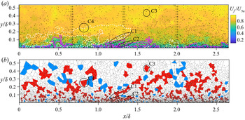
Figure 1(a) illustrates one snapshot of the instantaneous  $U$-component velocity field in the
 $x$–
 $y$ plane of case T1 that was stitched from the measurements of the four CCD cameras. Individual sand grains are superimposed in the figure to visualize the non-uniform particle distribution in the whole FOV. Such a plot infers the presence of particle structures, which will be quantified by the method of Voronoï tessellation.
(a) Instantaneous snapshot of  $U$-component velocity fields of the fluid phase in the
 $x - y$ plane in case T1. The black dashed lines denote the overlapped FOV between neighbouring CCD cameras. White dashed contours and magenta solid contours represent the detected positive and negative wall-attached
 $u$-structures following the detection criterion of Hwang & Sung (Reference Hwang and Sung2018), which will be discussed in § 4.2. (b) Voronoï diagrams of the particle distribution and the detected particle clusters (patches of connected cells in red) and particle voids (patches of connected cells in blue). Four clusters are marked as C1–C4, and their position is also indicated in panel (a). The black dots represent the sand grains, without an indication of their actual size.

3.1. Voronoï tessellation
In Voronoï analysis, the space occupied by discrete particles is divided into Voronoï cells, each of which is an independent polygon containing one particle inside it. The definition of a Voronoï cell makes the spatial points inside one cell have the closest distance to its interior particle than to any other exterior ones. Such a feature makes the space tessellation unique for one snapshot of the particle distribution. Figure 1(b) shows one example of the Voronoï tessellation. The area of a Voronoï cell is an ideal measure of the local particle concentration (Monchaux et al. Reference Monchaux, Bourgoin and Cartellier2010). The mean particle volume fraction at a spatial position of  $(x,y)$, i.e.
 $\phi _V(x,y)$, can be estimated by the mean area of Voronoï cells centred at
 $(x,y)$, i.e.
 \begin{gather} \phi_{Vi}(x_i,y_i,t)=\frac{V_p}{A_{ri}(x_i,y_i,t)\Delta z}, \end{gather}
 \begin{gather} \phi_{V}(x,y)=\frac{1}{M}\sum_{t=1}^M\left(\frac{1}{N_p(x,y,t)}\sum_{i=1}^{N_p}\phi_{Vi}(x_i,y_i,t)\right). \end{gather}
In (3.1),  $A_{ri}$ is the area of the Voronoï cell of the
 $i$th sand grain with centroid of
 $(x_i, y_i)$ at time instant
 $t$;
 $V_p={\rm \pi} d_p^3/6$ is the mean volume of one single sand grain with an idealized sphere shape;
 $\Delta z$ is the thickness of the illumination plane; and
 $\phi _{Vi}$ is the local particle volume fraction contributed by the
 $i$th sand grain. In (3.2),
 $\phi _{V}$ averages the contribution of all
 $N_p$ sand grains in
 $M$ snapshots whose centroids
 $(x_i,y_i)$ fall inside the probing box centred at
 $(x,y)$ with a bin of
 $\Delta x\times \Delta y$.
The local particle volume fraction can also be estimated by the conventional box-counting method (Aliseda et al. Reference Aliseda, Cartellier, Hainaux and Lasheras2002). This method divides the measurement domain into a group of probing boxes with sizes of  $\Delta x\times \Delta y$. The number of particles
 $N_p$ contained in each box is counted, and the local mean particle volume fraction
 $\phi _B$ is estimated as
 \begin{equation} \phi_{B}(x,y)=\frac{1}{M}\sum_{t=1}^M\frac{V_pN_p(x,y,t)}{\Delta x \Delta y \Delta z}. \end{equation}
The probing box is fixed as  $\Delta x^+\times \Delta y^+ =175\times 17.5$ for both methods. Averaging
 $\phi _{V \mid B} (x,y)$ across
 $x$ yields
 $\varPhi _{V \mid B} (y)$, which are shown in figure 2(a). The conditional particle volume fractions inside particle clusters and particle voids, i.e.
 $\varPhi _V^C$ and
 $\varPhi _V^V$, are also shown in figure 2(a) for comparison. These conditional quantities are to be discussed later. Hereinafter, the superscripts
 $C$,
 $V$ and
 $A$ indicate parameters conditioned inside particle clusters, voids and of all the events, respectively. Owing to the spatially developing nature of the two-phase flow,
 $\varPhi _{V \mid B} (y)$ is ensemble-averaged in a limited span of
 $1.7< x/\delta <2.3$. As shown in Appendix A, the streamwise variation of sand grains’ statistics over such a limited span is less prominent even in the near-wall region. It has been verified that shifting the probing span upstream will not change the shape of the yielded
 $\varPhi _{V \mid B}(y)$ profile, as well as other statistical quantities to be discussed later. Therefore, if without an explicit claim, this streamwise span is kept in all the following statistical analysis.
(a) Wall-normal profiles of local particle volume fraction being conditioned inside particle clusters ( $\varPhi _V^C$) or voids (
 $\varPhi _V^V$), as well as the unconditional ones (
 $\varPhi _V^A$), that are obtained by the Voronoï tessellation method. Here
 $\varPhi _B^A$ obtained by the box-counting method is also shown for comparison. The dash-dotted green lines indicate a power-law scaling of
 $\varPhi _{V \mid B} \propto y^{-1.2}$ in the log layer. (b) Wall-normal variation of the percentage of sand grains falling inside either clusters (
 $NP^C$) or voids (
 $NP^V$). Both cases T1 and T2 are shown, and the statistics are counted in the streamwise range of
 $1.7< x/\delta <2.3$. The shaded regions in panels (a) and (b) indicate the log layer of the TBL.

Figure 2(a) shows a good agreement between  $\varPhi _V^A (y)$ and
 $\varPhi _B^A (y)$ except for the flow layers very close to the lower or upper bound of the FOV, i.e.
 $y/\delta < 0.01$ or
 $y/\delta > 0.48$, where the accurate detection of the Voronoï cell suffers from contamination of the FOV boundary (Monchaux et al. Reference Monchaux, Bourgoin and Cartellier2010). To avoid the boundary contamination issue, those Voronoï cells that intersect with the boundary of the FOV are discarded from the ensemble in the following statistical analysis. As shown in figure 2(a),
 $\varPhi _V^A (y)$ presents a power-law decay of
 $\varPhi _V^A \propto y^{-1.2}$ in the upper half of the log layer, but deviates from it in both the near-wall region and the wake region. Such a deviation was also reported in the recent studies of particle-laden TBL (Berk & Coletti Reference Berk and Coletti2020). It is noted that the lower bound of the log layer is set as
 $y^+=3\sqrt {Re_\tau }=222$ (
 $y/\delta = 0.04$), while the upper bound is
 $y/\delta = 0.2$ (
 $y^+=1110$), a bit higher than the previously used values of
 $y/\delta =0.15 - 0.18$ (Marusic et al. Reference Marusic, Monty, Hultmark and Smits2013). The reason for such relaxation is that, as will be shown later, self-similarity of particle clusters can still be observed at this flow layer. Moreover, the mean velocity profiles
 $\bar {U}_f (y)$ in two particle-laden cases (cases T1 and T2) roughly follow the log law till
 $y/\delta= 0.2$.
According to the classical Rouse–Prandtl model (Rouse Reference Rouse1937; Prandtl Reference Prandtl1952), the vertical distribution of particle concentration in horizontal wall-bounded flow follows a power-law scaling, i.e.
 \begin{equation} \varPhi_B (y)/\varPhi_B (y_r)=(y/y_r)^{{-}Ro}, \end{equation}
in which  $\varPhi _B (y_r)$ is the particle concentration at an arbitrary reference height
 $y_r$. By considering the role of turbulent dispersion and gravitational settling in the process of particle sedimentation (Rouse Reference Rouse1937; Chamecki et al. Reference Chamecki, van Hout, Meneveau and Parlange2007), the Rouse number
 $Ro$ in the so-called Rouse profile of (3.4) was formulated as
 \begin{equation} Ro=S_cV_s/(\kappa u_\tau), \end{equation}
with  $V_s$ the particle settling velocity and
 $\kappa$ the von Kármán constant. The modification factor
 $S_c$ is the turbulent Schmidt number. It accounts for the weighting between eddy viscosity of the fluid phase and diffusivity of the particle phase, and thus measures the relative strength of turbulent transport. The particle diffusivity is influenced by both the effect of gravity (or the density ratio) and the particle inertia. In the case of fluvial sediment transport, where the particle–water density ratio is moderate, eddy viscosity and particle diffusivity can be close to each other; therefore,
 $S_c$ was usually assumed to be 1.0 (Rouse Reference Rouse1937; Rose & Thorne Reference Rose and Thorne2001). For the case of pollen transport in the ASL with small particle inertia, Chamecki & Meneveau (Reference Chamecki and Meneveau2011) estimated a magnitude of
 $S_c=0.4$. In order to accurately determine
 $S_c$, the particle diffusivity should be known in advance. It needs information about the particle Lagrangian velocity (Sabban & van Hout Reference Sabban and van Hout2011), which cannot be easily obtained in an experiment. As an alternative,
 $S_c$ was calibrated from the Rouse profile of (3.4) and (3.5) in previous studies (Rose & Thorne Reference Rose and Thorne2001; Chamecki et al. Reference Chamecki, van Hout, Meneveau and Parlange2007). Using the same approach, the turbulent Schmidt number is estimated to be
 $S_c\approx 0.1$ in the present case (given
 $Ro=1.2$ and
 $V_s\approx 1.1\ \textrm {m}\,\textrm {s}^{-1}$), falling in the range of
 $S_c=0.05 - 0.14$ that was reported by Farrell & Sherman (Reference Farrell and Sherman2013) in their study of sand-laden turbulent airflow. To our knowledge, such a small magnitude of
 $S_c$ infers a dominance of particle diffusivity over eddy viscosity. This might be reasonable, since the present two-phase flow has both high sand–air density ratio and large particle Stokes number.
3.2. Detection of particle structures
As suggested by Monchaux et al. (Reference Monchaux, Bourgoin and Cartellier2010), p.d.f.s of the normalized Voronoï cell area  $\gamma$ can be used to define particle clusters, where
 $\gamma$ is calculated as
 $\gamma \equiv A_r/\overline {A_r}$, with
 $\overline {A_r}$ the mean value of
 ${A_r}$. In wall-bounded turbulence, the distribution of sand grains presents non-uniformity along the wall-normal direction. Previous studies on two-phase TCF (Yuan et al. Reference Yuan, Zhao, Andersson and Deng2018) dealt with this issue by normalizing
 ${A_r}$ via the mean value at one flow layer and examining the
 $\gamma$–p.d.f. profiles layer by layer. This strategy is adopted here. Furthermore, to compensate for the streamwise developing feature in the present particle-laden flow, a slight modification was made to normalize
 $A_r$ by its local mean value
 $\overline {A_r}$ at each
 $(x, y)$ instead of by the layer mean value. Such a strategy has been used by Sumbekova et al. (Reference Sumbekova, Cartellier, Aliseda and Bourgoin2017) in their study of droplet-laden grid turbulence. Figure 3(a) shows the
 $\gamma$–p.d.f. profiles at different flow layers counted within
 $1.7< x/\delta <2.3$ in case T1. Each Voronoï cell is indexed by the spatial position of the sand grain inside it. The bin of one flow layer has a height of
 $\Delta y/\delta =0.01$, the same as in the following analysis. The ensemble size in each bin is more than
 $O(10^4)$ even at
 $y/\delta =0.32$. Since cases T1 and T2 always present similar behaviours in various aspects of the characteristics of particle clustering, the results of case T2 are not shown in figure 3 and the following figures without explicitly claiming so.
The p.d.f.s of (a) the dimensionless area  $\gamma =A_r/\overline {A_r}$ and (b) its transformed logarithmic axis at typical flow layers in case T1. In (a), the p.d.f. of a random Poisson process (RPP) is shown as a black dashed line, whose two intersections with the
 $\gamma$–p.d.f. profiles yield the thresholds
 $\gamma _C$ and
 $\gamma _V$ for particle clusters and voids, respectively. The two vertical shaded regions represent the range of the scattered values of
 $\gamma _C$ or
 $\gamma _V$ reported in previous studies on HIT and TCF. In (b), the red dashed line indicates a standard Gaussian distribution. Only ensembles in the range of
 $1.7< x/\delta <2.3$ are counted in the statistics, and the same is true in figures 4, 5, 11, 14, 15 and 16 and thus is not explicitly stated in the captions of these figures.

As shown in figure 3(a), the  $\gamma$–p.d.f. profiles at different flow layers fail to collapse onto each other. Instead, the left tails elevate with the increase of
 $y$. This is consistent with the recent observation by Fong et al. (Reference Fong, Amili and Coletti2019) in a particle-laden TCF. Nevertheless, replotting the
 $\gamma$–p.d.f. profiles on a normalized logarithmic axis, in which
 $\log (\gamma )$ is realigned with the mean value
 $\overline {\log (\gamma )}$ and rescaled by the standard deviation
 $\sigma _{log(\gamma )}$, leads to a satisfying collapse of all the profiles, as shown in figure 5(b). A comparison with the standard Gaussian profile suggests that
 $\gamma$–p.d.f. at each flow layer is close to a log-normal distribution with a slight deviation on the left tail. Note that the quasi-log-normal distribution of
 $\gamma$ was also observed in HIT (Monchaux et al. Reference Monchaux, Bourgoin and Cartellier2010; Obligado et al. Reference Obligado, Teitelbaum, Cartellier, Mininni and Bourgoin2014), but a reasonable explanation for the underlying mechanism is still lacking.
Similar to the cases in HIT and TCF (Monchaux et al. Reference Monchaux, Bourgoin and Cartellier2010; Rabencov & van Hout Reference Rabencov and van Hout2015), the  $\gamma$–p.d.f. profiles are compared with a random Poisson process (RPP) that has the approximate analytical expression
 \begin{equation} \text{p.d.f.}_{2D}(\gamma)=(343/15)\sqrt{7/2{\rm \pi}}\,\gamma^{5/2} \mathrm{e}^{{-}7\gamma/2}. \end{equation}
As shown in figure 3(a), there are always two intersections between the profiles of p.d.f.( $\gamma$) and of RPP. The
 $\gamma$ values of the left and right intersections are denoted as
 $\gamma _C$ and
 $\gamma _V$, respectively. Following Monchaux et al. (Reference Monchaux, Bourgoin and Cartellier2010),
 $\gamma _C$ is regarded as the upper bound of the non-dimensional area of Voronoï cells that belong to particle clusters, while
 $\gamma _V$ is the lower bound for Voronoï cells falling in particle voids, which were usually interpreted as the sparse counterpart of clusters. It is interesting to see that both
 $\gamma _C$ and
 $\gamma _V$ obtained here are insensitive to the wall-normal height. Their magnitudes fall in the scattering range of existing values (two shaded regions in figure 3a) that have been reported in HIT and TCF (Monchaux et al. Reference Monchaux, Bourgoin and Cartellier2010; Obligado et al. Reference Obligado, Teitelbaum, Cartellier, Mininni and Bourgoin2014; Rabencov & van Hout Reference Rabencov and van Hout2015; Baker et al. Reference Baker, Frankel, Mani and Coletti2017). Furthermore, it has been verified that
 $\gamma _C$ and
 $\gamma _V$ are independent of the streamwise span for statistical counting.
Using  $\gamma _C$ and
 $\gamma _V$, all the Voronoï cells in one snapshot can be marked as candidates of clusters, voids or neither. Connecting those neighbouring Voronoï cells with the same attribute forms the corresponding particle structures. As in Petersen et al. (Reference Petersen, Baker and Coletti2019), those particle structures containing less than three sand grains (or Voronoï cells) were rejected in the subsequent statistical counting. Figure 1(b) shows particle structures by coloured Voronoï cells. It is seen that a large fraction of particle clusters presents a rod-like pattern inclining away from the wall (see those marked as C1 and C2 in figure 1(b), for instance). Such a pattern is rarely seen in particle voids. It seems to resemble the geometrical characteristics of the so-called attached eddies (Hwang & Sung Reference Hwang and Sung2018; Marusic & Monty Reference Marusic and Monty2019). This aspect will be addressed later in § 4.2.
Figure 2(b) shows the number percentage  $NP^{C \mid V}$ of sand grains belonging to particle clusters or voids as a function of wall-normal height. As shown in figure 2(b),
 $NP^C$ is always larger than
 $NP^V$. Both are only weakly dependent on
 $y$ in the log layer and above. This is in distinct contrast to the trend of the quick growth of
 $NP^{C \mid V}$ below
 $y/\delta =0.02$, where the relatively low magnitude of
 $NP^{C \mid V}$ might be attributed to the enhanced inter-particle collisions and particle–wall collisions that randomize the dispersion of sand grains in the near-wall region. Note that, in the log layer and above,
 $NP^C \approx 20\,\%$ is comparatively larger than that reported in previous studies (Baker et al. Reference Baker, Frankel, Mani and Coletti2017; Petersen et al. Reference Petersen, Baker and Coletti2019). This might be attributed to the large
 $St_p$ (
 $\sim O(10^2 - 10^3)$) in the present experiment, since Baker et al. (Reference Baker, Frankel, Mani and Coletti2017) reported that, in HIT,
 $NP^C$ increased from
 $3\,\%$ to
 $14\,\%$ when
 $St_p$ changed from
 $O(10^0)$ to
 $O(10^1)$. We would like to emphasize that even with
 $NP^C \approx 20\,\%$, particle structures are still low-probability events.
The wall-normal profiles of the conditional particle volume fraction  $\varPhi _V^{C \mid V}$, which are obtained via (3.1) and (3.2) by counting only samples inside particle clusters (or voids), are also shown in figure 2(a). For each flow layer,
 $\varPhi _V^C$ is one order of magnitude larger than
 $\varPhi _V^V$. Both present a power-law decay in the log layer, with the power index being
 $Ro=1.2$, the same as that of the
 $\varPhi _V^A (y)$ profiles. To our knowledge, such an agreement has a two-fold explanation. First, the particle clusters only occupy a small fraction of the whole sand-grain ensemble; therefore, it is less possible that they are able to bias the mean particle concentration. Second and perhaps more likely, as has been stated earlier, the relatively small magnitude of
 $S_c$ suggests that, in the flow region away from the wall, the particles’ bulk distribution is mainly characterized by the joint effect of gravitational settling and particle inertia. This is consistent with the findings in Richter & Chamecki (Reference Richter and Chamecki2018) and Berk & Coletti (Reference Berk and Coletti2020). On the other hand, turbulent coherent motions play a role of affecting the sand grains’ instantaneous distribution, and thus contribute to the formation of particle clusters and voids. Referring to the above observation that
 $NP^{C}$ and
 $NP^{V}$, as well as their ratio, are quasi-constant in the flow region where
 $\varPhi _V^A \propto y^{-Ro}$ holds, it can be inferred that particle structures might not be a global vertical flux but local events under the net sedimentation condition. Concretely, particle clusters and voids at the same flow layer balance well with each other and make no net contribution to the bulk particle concentration. In this sense, the observation that the profiles of
 $\varPhi _V^{C \mid V}(y)$ only present a vertical shift from
 $\varPhi _V^{A}(y)$ without a change of the Rouse number can be expected.
3.3. Fractal characteristics of particle structures
Figure 4(a,b) map the square root of the area  $\sqrt {A_C}$ of each cluster with respect to its perimeter
 $P_C$ at
 $y/\delta =0.06$ and 0.18 in case T1, while figure 4(d,e) plot
 $\sqrt {A_V}\sim P_V$ of particle voids at the same flow layer. Such a map serves as a diagnostic tool to reveal the fractal characteristics of the geometries of particle clusters (or voids).
Scatter plot of ( $\sqrt {A_{C \mid V}}$,
 $P_{C \mid V}$ ) of each cluster or void at (a,d)
 $y/\delta =0.06$ and (b,e)
 $y/\delta =0.18$ in case T1. The superimposed contours in a logarithmic scaling in (a,b,d,e) represent the j.p.d.f.s, while the black dashed lines indicate the most probable
 $A_C^{mop}$ or
 $A_V^{mop}$ to be shown in figure 5. (c, f) Wall-normal variation of the exponents
 $E_{C1 \mid V1}$ and
 $E_{C2 \mid V2}$ in cases T1 and T2. The error bars in (c, f) represent the uncertainty in estimating
 $E_{C1 \mid V1}$ and
 $E_{C2 \mid V2}$ via a least-squares fitting. The horizontally shaded regions in (c) indicate the scattered ranges of
 $E_{C1}$ and
 $E_{C2}$ that have been reported in previous studies on HIT and TCF.

Figure 4(a,b) reveal two different scalings of the right envelope of the fractal chart, i.e.  $\sqrt {A_C}\sim P_C^{E_1}$ for small and compact clusters, and
 $\sqrt {A_C}\sim P_C^{E_2}$ for large and fractal ones. Such a two-branch pattern holds for all the flow layers being investigated here. This was also observed in previous studies on HIT and TCF. Figure 4(c) summarizes the magnitude of
 $E_{C1}$ and
 $E_{C2}$ of particle clusters at various wall-normal heights in cases T1 and T2, in which the two shaded regions indicate the scattered ranges of the existing data reported in HIT and TCF via numerical simulations or experiments (Aliseda et al. Reference Aliseda, Cartellier, Hainaux and Lasheras2002; Monchaux et al. Reference Monchaux, Bourgoin and Cartellier2010; Obligado et al. Reference Obligado, Teitelbaum, Cartellier, Mininni and Bourgoin2014; Rabencov & van Hout Reference Rabencov and van Hout2015; Baker et al. Reference Baker, Frankel, Mani and Coletti2017). The
 $E_{C1}$ value obtained here is seen to asymptote to 1.0 once beyond the upper bound of the log layer (
 $y/\delta =0.2$). The asymptotic state of
 $E_{C1}\sim 1.0$ indicates regular geometries of 2-D objects (particle clusters marked as C3 and C4 in figure 1(b), for instance). Furthermore,
 $E_{C2}$ is approximately 2.0 in the near-wall region and decreases monotonically with an increase in
 $y$. The relatively large magnitude of
 $E_{C2}$ suggests the corrugated fractal nature of the periphery of particle clusters (see those marked as C1 and C2 in figure 1(b), for instance). It is noted that previous studies related particle clusters with a larger fractal dimension to turbulent structures, which also present a fractal nature (Carter & Coletti Reference Carter and Coletti2018). The relaxation of
 $E_{C2}$ towards the values observed in HIT (pink shaded region in figure 4c) can be attributed to the gradual diminishing of the wall effect in the outer layer where the inhomogeneity of turbulent motions is relaxed.
As for particle voids, a pattern of two branches also appears in the fractal charts of figure 4(d,e). Compared with particle clusters, the fractal dimensions  $E_{V1}$ and
 $E_{V2}$ (shown in figure 4f) presents different wall-normal variations. Namely,
 $E_{V1}$ increases with
 $y$ and asymptotically converges to 1.3 in the wake region, while
 $E_{V2}$ scatters around 1.9 without a clear descending trend. Furthermore, the spreading in the (
 $\sqrt {A_C}$,
 $P_V$) map, as can be inferred from the joint probability distribution functions (j.p.d.f.s) superimposed in figure 4(d,e), is less prominent than that of particle clusters, suggesting the comparatively narrower scale range embedded in particle voids. This reveals a different geometric feature between clusters and voids, which will be further addressed below.
3.4. Geometrical self-similarity of particle clusters
Using Voronoï tessellation and the detection criterion developed above, the wall-normal variation of the geometries of particle clusters and voids will be studied. Here, the focus is on the existence of a self-similarity of the former in the log layer.
P.d.f.s of the area  $A_C$ of particle clusters at various flow layers of case T1 in the range of
 $1.7< x/\delta <2.3$ are shown in figure 5. For a direct comparison, p.d.f.s of both the area
 $A_r$ of Voronoï cells and the area
 $A_V$ of particle voids are also shown. The multiscale nature of the preferential particle concentration can be seen from the wide spread of p.d.f.(
 $A_C$) and p.d.f.(
 $A_V$). Interestingly, a scaling of
 $y\delta$ for
 $A_C$, instead of an outer scaling of
 $\delta ^2$, collapses the profiles of p.d.f.(
 $A_C/y\delta$) in the range of
 $0.04\leq y/\delta \leq 0.32$ on the right-hand side of the most probable value
 $A_C^{mop}$, where a power-law decay with a power index of
 $-5/3$ is evident in a wide scale range. In contrast, p.d.f.(
 $A_C/y\delta$) below the log layer (at
 $y/\delta =0.02$ in figure 5e) deviates from the
 $-5/3$ power-law decay when
 $A_C/y\delta > 0.02$. Neither the scaling of
 $\delta ^2$ nor that of
 $y\delta$ works for p.d.f.(
 $A_r$) and p.d.f.(
 $A_V/y\delta$) in a wide flow region; furthermore, p.d.f.(
 $A_V/y\delta$) presents a
 $-5/3$ power-law decay in a scale range much narrower than that in p.d.f.(
 $A_C/y\delta$). Again, it is stressed that the spatially developing feature of the particle motion does not change the above observation, since we have checked that the profiles of p.d.f.(
 $A_C/y\delta$) being probed at various streamwise stations (with the same span) still present notable self-similarity resembling that shown in figure 5(e).
The p.d.f.s of (a,d)  $A_r$ of Voronoï cells, (b,e)
 $A_C$ of particle clusters and (c, f)
 $A_V$ of particle voids at typical wall-normal heights, all of which are normalized by
 $\delta ^2$ in (a–c) and by
 $y\delta$ in (d–f). The bold dashed lines in (d–f) indicate a
 $-5/3$ power law, and the vertical dash-dotted lines in (e, f) indicate the most probable area
 $A_C^{mop}$ or
 $A_V^{mop}$.

Note that the  $-5/3$ power law was observed in the area distribution of particle clusters in HIT (Obligado et al. Reference Obligado, Teitelbaum, Cartellier, Mininni and Bourgoin2014; Baker et al. Reference Baker, Frankel, Mani and Coletti2017; Monchaux & Dejoan Reference Monchaux and Dejoan2017; Sumbekova et al. Reference Sumbekova, Cartellier, Aliseda and Bourgoin2017). As for two-phase wall-bounded turbulence, only Rabencov & van Hout (Reference Rabencov and van Hout2015) reported a
 $-2$ power-law scaling of particle clusters’ area distribution in TCF. The present observed
 $y$-scaling and
 $-5/3$ power law clearly indicate a self-similarity of the scales of particle clusters. Furthermore, the most probable area
 $A_C^{mop}$ is shown in figure 4(a,b) (as vertical black dashed lines) to show that the upper branch of the (
 $\sqrt {A_C}, P_C$) map, which has a higher fractal dimension, falls completely in the self-similar scale range of p.d.f.(
 $A_C$). This is again consistent with previous observations in HIT (Baker et al. Reference Baker, Frankel, Mani and Coletti2017; Sumbekova et al. Reference Sumbekova, Cartellier, Aliseda and Bourgoin2017; Petersen et al. Reference Petersen, Baker and Coletti2019).
The self-similarity of the areas of particle clusters can be further evidenced by the wall-normal variation of the statistical moments, i.e. the mean area  $\overline {A_C}$ and the standard deviation
 $\sigma _{A_C}$. Figure 6 shows the first two moments of
 $A_r$,
 $A_C$ and
 $A_V$ for comparison. The statistical results counted in two streamwise ranges, i.e.
 $0.3< x/\delta <0.9$ (solid lines) and
 $1.7< x/\delta <2.3$ (dotted lines), are presented to show that non-equilibrium of the particle motion in the near-wall region has a minor effect. For particle clusters,
 $\overline {A_C}/y\delta$ is seen to be quasi-constant across the log layer, indicating a linear relation of
 $\overline {A_C}\propto y$. The value of
 $\sigma _{A_C}/y\delta$ fails to present a plateau in the log layer, but the variation is mild when compared with those of
 $\sigma _{A_r}/y\delta$ and
 $\sigma _{A_V}/y\delta$. Owing to the slow convergence of the second-order moment and its sensitivity to extreme events, it is acceptable to approximate a quasi-linear scaling of
 $\sigma _{A_C}\propto y$ in the log layer. In contrast, neither Voronoï cells nor particle voids present a similar
 $y$-scaling behaviour of
 $\bar {A}_{V \mid r}$ and
 $\sigma _{A_{V \mid r}}$, consistent with the observations in p.d.f.(
 $A_r$) and p.d.f.(
 $A_V$) (shown in figure 5).
Wall-normal variation of (a) the normalized mean area  $\overline {A_{*}}/y\delta$ (
 $\overline {A_{*}}=\overline {A_{C}},\ \overline {A_{V}}$ or
 $\overline {A_{r}}$) and (b) their standard deviation
 $\sigma _{A_{*}}/y\delta$ in cases T1 and T2. Hollow or solid symbols with solid lines or dotted lines denote the statistics counted in the range of
 $0.3 < x/\delta < 0.9$ or
 $1.7< x/\delta <2.3$, respectively.

Finally, it is emphasized that the conditional particle volume fraction  $\varPhi _V^C$ at one flow layer is not equivalent to the inverse of the mean area of particle clusters
 $\overline {A_C}$ there. By definition, the former counts the area
 $A_r$ of individual Voronoï cells that belong to particle clusters in the ensemble average process, while, in the latter, several
 $A_r$ pertaining to one particle cluster are summed up to yield
 $A_C$. Therefore, there is no conflict between the two observed scalings, i.e.
 $\varPhi _V^C \sim y^{-1.2}$ and
 $\overline {A_C}\sim y$, since the average number of sand grains belonging to one particle cluster varies with
 $y$.
4. Correlation between particle clusters and wall-attached structures
4.1. A conceptual model
For HIT, the self-similarity of particle clusters was attributed to the self-similarity of fluid-phase coherent eddies across the inertial subrange of turbulent energy cascade (Goto & Vassilicos Reference Goto and Vassilicos2008; Baker et al. Reference Baker, Frankel, Mani and Coletti2017). As stated in § 1, for wall-bounded two-phase flows, previous studies mainly focused on the correlation between low-speed streaks and particle clusters in the near-wall region. In contrast, knowledge on the mechanisms of the formation of particle structures in the outer region, as well as their relationship with multiscale self-similar turbulent structures, is comparatively less.
In single-phase wall-bounded turbulence with high Reynolds number, the log layer is the flow region where the mean streamwise velocity, the even-order moments of the streamwise fluctuating velocity, the structure functions and the moment generating functions all present a logarithmic dependence on the wall-normal height (Marusic et al. Reference Marusic, Monty, Hultmark and Smits2013; Meneveau & Marusic Reference Meneveau and Marusic2013; Yang et al. Reference Yang, Meneveau, Marusic and Biferale2016, Reference Yang, Baidya, Johnson, Marusic and Meneveau2017b). A classic interpretation for the log law is the attached eddy hypothesis (AEH; Townsend Reference Townsend1976), which represents the velocity fluctuations in the log layer by the superposition of a hierarchy of inviscid wall-attached eddies. The unique feature of these attached eddies is that they are self-similar in such a way that their geometric size scales with  $y$ and their population densities are inversely proportional to
 $y$ (Marusic & Monty Reference Marusic and Monty2019). Since a
 $y$-scaling is also observed in the size of self-similar particle clusters in the log layer of the present studied particle-laden TBL, it is reasonable to infer a correlation between attached eddies and particle clusters.
With this background, a conceptual model is proposed in figure 7. It assumes that a significant proportion of particle clusters reside on the ridges of negative  $u$-structures that are attached to the wall. Such a pattern can be visualized in figure 1(b) as the regions C1 and C2. It is emphasized that this simplified model ignores several factors that might have direct influence on the preferential particle concentration, such as particle saltation, inter-particle collisions and induction of small-scale vortical structures. Nevertheless, the essence of this model is to provide a rudimental explanation for the self-similarity of particle clusters in the log layer. In the following, various pieces of evidence will be provided in favour of it.
A conceptual model for the spatial correlation between particle clusters and wall-attached structures.

4.2. Self-similar wall-attached  $u$-structures

Before presenting evidence to support this conceptual model, it is necessary to quantify whether the particle-laden condition alters the statistical and kinematical characteristics of wall-attached eddies.
The spectral characteristics of fluctuating velocities might provide the first clue. Figure 8 compares the pre-multiplied streamwise spectrograms of fluid-phase  $u_f$ and
 $v_f$ components, i.e.
 $k_x\varPhi _{uu}(y^+,\lambda _x^+)$ and
 $k_x\varPhi _{vv}(y^+,\lambda _x^+)$, in cases S, T1 and T2. Such spectrograms are obtained from the streamwise series of u f(x; y) or
 $v_f(x; y)$ layer by layer. The near-wall non-equilibrium condition in the particle-laden cases was ignored for a leading-order estimation, but
 $u_f$ and
 $v_f$ were calculated by subtracting their local mean value. To our knowledge, using spatial signals of the large-field PIV dataset is the most practical solution for obtaining the spectra of two-phase turbulent flow experimentally. Owing to the limited streamwise span (
 $\Delta X=2.67\delta$), the scales related with LSMs and very large-scale motions (VLSMs) cannot be fully resolved. Despite this limitation, the outer spectral peak in
 $k_x\varPhi _{uu}$ is still partly visualized. The presence of particle motion is seen to shift the near-wall energetic scales in
 $k_x \varPhi _{uu}$ from
 $\lambda _x^+\approx 1000$ to
 $\lambda _x^+\approx 200 - 300$, while the outer spectral peak is found to be less affected. More importantly, the intermediate region connecting the inner and outer peak in
 $k_x \varPhi _{uu}$, which follows a
 $\lambda _x^+=3.5y^+$ scaling (yellow dash-dotted lines in figure 8a–c) as proposed by Agostini & Leschziner (Reference Agostini and Leschziner2017), remains untouched in the particle-laden cases. Finally, the footprint of wall-attached eddies can also be inferred from the
 $v_f$-component spectra
 $k_x\varPhi _{vv}(y^+,\lambda _x^+)$ in cases T1 and T2, in which the spectral ridges roughly follow a scaling of
 $\lambda _x^+=2y^+$ (blue dashed straight lines in figure 8d–f) that has been reported in single-phase TBLs (Baidya et al. Reference Baidya, Philip, Hutchins, Monty and Marusic2017).
The pre-multiplied streamwise energy spectra of (a–c) the streamwise fluctuating velocity and (d–f) the wall-normal fluctuating velocity: (a,d) case S, (b,e) case T1 and (c, f) case T2. The coloured contours are the spectra  $k_x \varPhi _{uu}/u_\tau ^2$ and
 $k_x \varPhi _{vv}/u_\tau ^2$ of the original velocity fields, the red solid contours are the conditional spectra
 $k_x \varPhi _{uu}^C/u_\tau ^2$ and
 $k_x \varPhi _{vv}^C/u_\tau ^2$ inside particle clusters, and the black dashed contours are the conditional spectra
 $k_x \varPhi _{uu}^V/u_\tau ^2$ and
 $k_x \varPhi _{vv}^V/u_\tau ^2$ inside particle voids. The yellow and green dash-dotted straight lines in (a–c) denote the scaling of
 $\lambda _x^+=3.5 y^+$ and
 $\lambda _x^+=0.35 y^+$, respectively. The blue dashed lines in (d–f) denote
 $\lambda _x^+=2 y^+$. The grey shaded region in each panel indicates the range of the log layer of the TBL.

Following Hwang & Sung (Reference Hwang and Sung2018), we focus on wall-attached  $u$-structures in physical space. Attached
 $u$-structures are defined as connected regions with high levels of streamwise fluctuating velocities, i.e.
 $| u(x,y) | >\alpha u_{rms}(y)$, that are ‘attached’ to the wall. Owing to the 2-D measurement limitation, only 2-D slices of three-dimensional (3-D) physical structures can be detected. Those structures that are connected outside the observation plane will be rejected. Nevertheless, the detected 2-D slices are guaranteed to belong to 3-D wall-attached structures (a sufficient but unnecessary condition), so that the planar geometrical characteristics of the latter can be approximated by the former if statistical convergence is achieved. After a percolation test as recommended by Lozano-Durán, Flores & Jiménez (Reference Lozano-Durán, Flores and Jiménez2012) and Hwang & Sung (Reference Hwang and Sung2018), the threshold factor
 $\alpha$ is set to be 1.5. A mild variation of
 $\alpha$ will not qualitatively change the self-similar characteristics of those detected structures. Finally, the condition of wall attachment invoked here is similar to that used by Lozano-Durán et al. (Reference Lozano-Durán, Flores and Jiménez2012). Namely, the minimum height for attached
 $u$-structures is the secondary resolved flow layer above the wall, i.e.
 $y_{smin}/\delta =0.006$ or
 $y_{smin}^+ =34$.
Wall-attached positive or negative  $u$-structures being detected by the above criteria are illustrated as solid or dashed contours in figure 1(a). It is shown that a large proportion of them incline away from the wall and extend into the outer layer. Figure 9 shows the wall-normal variation in both the ensemble-averaged area
 $\overline {A_u}$ of attached
 $u$-structures and their standard deviation
 $\sigma _{A_u}$ in cases T1 and T2. The result of the baseline case S is also shown for comparison. Similar to particle clusters, attached
 $u$-structures are indexed by their geometric centroids, with a bin height of
 $\Delta y/\delta = 0.01$ for statistical counting.
Wall-normal variation of (a) the normalized mean area  $\overline {A_u}/y\delta$ and (b) the corresponding standard deviation
 $\sigma _{A_u}/y\delta$ of wall-attached
 $u$-structures in cases S, T1 and T2. Owing to the moderate- to large-scale nature of the attached eddies, as well as the approximate streamwise homogeneity of fluid-phase motion in the log layer and above, the whole streamwise span of the FOV is used for statistics.

For case S, a scaling of  $\overline {A_u} \propto y^2$ is presented below
 $y/\delta$ = 0.2. If the heights of attached
 $u$-structures are assumed to scale with
 $y$,
 $\overline {A_u} \propto y^2$ suggests that on average their streamwise length scales are linearly dependent on
 $y$. This is consistent with the primary assumption of linear scaling in AEH (Marusic & Monty Reference Marusic and Monty2019). For particle-laden cases, a remarkable deviation from the quadratic scaling of
 $\overline {A_u} \propto y^2$ is seen in the near-wall region: the higher the bulk particle volume fraction
 $\varPhi _{1}$, the larger is the deviation. To our knowledge, this fact might be explained by the suppression of small-scale turbulent fluctuation in the near-wall region due to the high particle concentration there (as shown in figure 8). Namely, high-concentration sand grains ‘break’ attached
 $u$-structures into fragments by an enhanced turbulent modulation effect, thus reducing the size of attached
 $u$-structures being detected by the present 2-D probing method. It is unknown whether such a deviation is still evident when 3-D attached
 $u$-structures are detected by a 3-D connectivity criterion. Nevertheless, even in the present 2-D case,
 $\overline {A_u}$ gradually converges to that of case S in the log layer and above. This implies that attached
 $u$-structures are less affected by particle motions in this region. Furthermore,
 $\sigma _{A_u}(y)$ of case S presents a similar quadratic scaling, i.e.
 $\sigma _{A_u}(y)\propto y^2$, which is asymptotically approached by
 $\sigma _{A_u}(y)$ of two particle-laden cases in the log layer and above.
Based on these observations, it can be inferred that, in the log layer and above, wall-attached turbulent structures with intermediate length scales are not significantly affected by the presence of particle motions. Note that there is a viewpoint that, in wall-bounded turbulence, large-scale structures such as LSMs and VLSMs are likely to be independent of the inner-layer cycle between streamwise vortices and low-speed streaks, especially when the scale separation is sufficiently large (Jiménez Reference Jiménez2018; Marusic & Monty Reference Marusic and Monty2019; Hu, Yang & Zheng Reference Hu, Yang and Zheng2020). In other words, ‘large-scale motions are themselves self-sustained’ (Rawat et al. Reference Rawat, Cossu, Hwang and Rincon2015). Therefore, it is reasonable to argue that, in the present particle-laden cases with dilute particle volume fraction, the alternation of near-wall turbulent statistics and structures, which mainly manifests in the small-scale range, might not severely affect large-scale turbulent structures in the outer region.
4.3. Evidence for the conceptual model: stretching of particle clusters
To our knowledge, the conceptual model shown in figure 7 is actually an exemplification of the large-scale centrifugal effect associated with high rate of strain (Bragg et al. Reference Bragg, Ireland and Collins2015b). Deng et al. (Reference Deng, Pan, Wang and He2018) have shown that bulge-like large-scale structures with negative  $u$-fluctuation represent a low-order footprint of hairpin packets, whose backward envelopes are characterized as interfaces of pairs of converging ejection–sweep (Q2–Q4) events. In such a picture, the converging Q2–Q4 events provide a source of strong strain and thus constitute one of the key features of the conceptual model, i.e. the preferential alignment of particle clusters to large-scale Q2–Q4 interfaces.
Owing to the sparsity nature of particle clusters and their versatile sizes, geometries and positions, it is impracticable to devise a suitable condition to obtain a conditionally averaged flow field resembling the flow pattern outlined in figure 7. Therefore, a conditional quadrant analysis is attempted. Figure 10(a) (or figure 10b) compares the j.p.d.f.s of  $(u_f, v_f)$ of the fluid phase being conditioned inside particle clusters (or voids) with those of the unconditional ones at
 $y/\delta = 0.06$ in case T1. Figure 10(c–f) plot their differences, i.e.
 $\mathrm {j.p.d.f.}(u_f^{C \mid V},v_f^{C \mid V}) - \mathrm {j.p.d.f.}(u_f^{A},v_f^{A})$, at
 $y/\delta$ = 0.06 and 0.18, to highlight the relative change of quadrant events due to the presence of particle clusters (or voids).
Strength of fluid-phase sweep and ejection events conditioned inside particle structures: (a) j.p.d.f. $(u_f^{A},v_f^{A})$ (black solid contour) and j.p.d.f.
 $(u_f^{C},v_f^{C})$ (red dashed contour) at
 $y/\delta =0.06$; (b) j.p.d.f.
 $(u_f^{A},v_f^{A})$ (black solid contour) and j.p.d.f.
 $(u_f^{V},v_f^{V})$ (blue dotted contour) at
 $y/\delta =0.06$; (c,e)
 $\mathrm {j.p.d.f.}(u_f^{C},v_f^{C}) - \mathrm {j.p.d.f.}(u_f^{A},v_f^{A})$ at
 $y/\delta =0.06$ and 0.18, respectively; and (d, f)
 $\mathrm {j.p.d.f.}(u_f^{V},v_f^{V}) - \mathrm {j.p.d.f.}(u_f^{A},v_f^{A})$ at
 $y/\delta =0.06$ and 0.18, respectively. The contour level in (a,b) varies from 0.02 to 0.08 with an interval of 0.02. Owing to the convergence consideration, the whole streamwise span of the FOV is used for statistics, and fluctuating velocities are presented in inner scaling.

Figure 10(c) presents the positive region of  $\mathrm {j.p.d.f.}(u_f^{C},v_f^{C}) - \mathrm {j.p.d.f.}(u_f^{A},v_f^{A})$ around the origin (
 $u_f=0, v_f=0$) at
 $y/\delta =0.06$, indicating that a comparatively higher probability of weak quadrant events (or lower probability of extreme quadrant events) occurs inside particle clusters. This is in accordance with the conceptual model (in figure 7), since the interface of converging Q2–Q4 events around back ridges of negative
 $u$-structures has weak strength of Reynolds shear stress. In contrast, figure 10(d) reveals a reverse trend for particle voids, i.e. the occurrence probability now spreads towards extreme quadrant events. At
 $y/\delta =0.18$ (in figure 10e, f), both j.p.d.f.
 $(u_f^{C},v_f^{C})$ and j.p.d.f.
 $(u_f^{V},v_f^{V})$ converge towards the unconditional j.p.d.f.
 $(u_f^{A},v_f^{A})$, but the overshot of the probabilities of weak (or strong) quadrant events inside particle clusters (or voids) is still observable.
The preferential alignment of particle clusters along the interface of converging Q2–Q4 events, if it is true, infers a trend of stretching of particle clusters along the interface. This inference is supported by figure 11, which shows the wall-normal variation of the ensemble-averaged length of the major (long) and minor (short) principal axes of particle clusters ( $\overline {L_{aC}}$ and
 $\overline {L_{bC}}$ ), as well as their slenderness ratio
 $\overline {S_C} =\overline {L_{aC}/L_{bC}}$. The corresponding values of particle voids (
 $\overline {L_{aV}}$,
 $\overline {L_{bV}}$ and
 $\overline {S_{V}}$) are also given for comparison. The principal axes of particle structures are obtained by elliptical fitting of their peripheries. Again, only particle structures in the range of
 $1.7< x/\delta <2.3$ are counted. In the log layer, both
 $\overline {L_{aC}} ^2$ and
 $\overline {L_{bC}}^2$ normalized by a mixed length scale of
 $y\delta$ are quasi-constant (shown in figure 11a). This is in distinct contrast to the monotonic growth of
 $\overline {L_{aV}}^2/y\delta$ and
 $\overline {L_{bV}}^2/y\delta$ there. It indicates a scaling of
 $\overline {L_{aC}}$ ∝
 $y^{1/2}$ and
 $\overline {L_{bC}}$ ∝
 $y^{1/2}$ and a quasi-invariant
 $\overline {S_C}$, the latter of which is more prominent in case T1 (shown in figure 11b). The relatively high magnitude of
 $\overline {S_C}$ (
 $\overline {S_C}> 4$) suggests a rod-like pattern of particle clusters in a statistical sense, as is shown by C1 and C2 in figure 1. It is noted that the scaling of
 $\overline {L_{aC \mid bC}}$ ∝
 $y^{1/2}$ is consistent with the linear dependence of
 $\overline {A_C}$ on
 $y$ if
 $\overline {A_C}$ is approximated by
 $\overline {L_{aC}} \times \overline {L_{bC}}$ for a regular shape.
Wall-normal variation of (a) the square of the mean length of the long and short principal axes  $\overline {L_{a}}^2$ and
 $\overline {L_{b}}^2$ of particle clusters or particle voids and (b) the mean slenderness ratio
 $\overline {S_C} =\overline {L_{a}/L_{b}}$ in cases T1 and T2.

According to the conceptual model shown in figure 7, the rapid increase in  $\overline {S_C}$ in the near-wall region (shown in figure 11b) can be explained by the strong rate of strain around the interfaces of converging Q2–Q4 events that play a role of stretching particle clusters along the interfaces. The ending of the quick growth of
 $\overline {S_C}$ in the log layer implies the attenuation of the stretching effect, which is attributed to the relaxation of the strength of backward induction from matured wall-attached eddies (Deng et al. Reference Deng, Pan, Wang and He2018). Instead, those particle clusters that are entrapped by attached eddies passively follow their wall-normal growth in a self-similar way.
The next piece of evidence is the correlation between the scales of particle clusters and the surrounding rate of strain in the fluid phase. Figure 12 compares j.p.d.f. $(A_C/\overline {A_C}, \tilde {S}_z/\overline {\tilde {S}_z})$ of particle clusters to j.p.d.f.
 $(A_r/\overline {A_r}, \tilde {S}_z/\overline {\tilde {S}_z})$ of Voronoï cells in two different flow regions, i.e. below the log layer with
 $y/\delta <0.04$ and in the log layer with
 $0.04\leq y/\delta < 0.2$, in case T1. Here
 $\tilde {S}_z$ is the spanwise component of the large-scale rate of strain of the fluid phase, i.e.
 $\tilde {S}_z= | \partial \tilde {v}_f/\partial x+\partial \tilde {u}_f/\partial y|$. Large-scale velocity components (
 $\tilde {u}_f$,
 $\tilde {v}_f$) are obtained by reconstructing the first six proper orthogonal decomposition (POD) modes of the original velocity fields. The reason for choosing such a POD-based filter is that it is adequate to delineate the kinematics of LSMs while minimizing the contamination of small-scale irregular fluctuations (Deng et al. Reference Deng, Pan, Wang and He2018). In the j.p.d.f.s,
 $\tilde {S}_z$ takes the mean value averaged inside each particle cluster or Voronoï cell. The denominators
 $\overline {A_C}$ and
 $\overline {\tilde {S}_z}$ are both averaged across one flow layer. The reason for taking into account a large flow domain instead of only one flow layer is to enlarge the ensemble size for the convergence of the j.p.d.f.s.
The j.p.d.f.s of the dimensionless area  $A_C$ or
 $A_r$ and the large-scale component of the rate of strain in the flow region (a) below the log layer with
 $y/\delta < 0.04$ and (b) of the log layer with
 $0.04 \leq y/\delta < 0.2$ in case T1. The black dashed contours indicate j.p.d.f.(
 $A_C/\overline {A_C}, \tilde {S}_z/\overline {\tilde {S}_z}$) of particle clusters and the coloured patches indicate j.p.d.f.(
 $A_r/\overline {A_r}, \tilde {S}_z/\overline {\tilde {S}_z}$) of all the Voronoï cells. Owing to the convergence consideration, the whole streamwise span of the FOV is used for statistics.

Owing to the nature of enhanced particle concentration in particle clusters, the j.p.d.f. $(A_C/\overline {A_C}, \tilde {S}_z/\overline {\tilde {S}_z})$ is left shifted towards the small-value side of the
 $A_C/\overline {A_C}$ axis when compared with the j.p.d.f.
 $(A_r/\overline {A_r},\tilde {S}_z/\overline {\tilde {S}_z})$. Importantly, the spreading of j.p.d.f.
 $(A_C/\overline {A_C},\tilde {S}_z/\overline {\tilde {S}_z})$ towards the positive side of the
 $\tilde {S}_z/\overline {\tilde {S}_z}$ axis is more prominent than that in j.p.d.f.
 $(A_r/\overline {A_r},\tilde {S}_z/\overline {\tilde {S}_z})$. This observation holds for both flow regions being probed. This suggests that, in a statistical sense, particle clusters are prone to appear in regions with strong rate of strain, which is again consistent with the conceptual model (in figure 7).
4.4. Evidence for the conceptual model: conditional spectrum
Conditional fluid-phase spectrograms  $k_x \varPhi _{uu}^{C \mid V}(\lambda _x,y)$ or
 $k_x \varPhi _{vv}^{C \mid V}(\lambda _x,y)$ associated with particle clusters or voids are superimposed onto the original spectra in figure 8 (red solid contours for
 $u$-component spectra or black dashed contours for
 $v$-component spectra) to examine whether kinematic self-similarity of wall-attached turbulent structures is exemplified in flow regions occupied by particle structures. Such conditional spectra are calculated by the following procedure. First, the whole fluid-phase velocity fields were masked by the peripheries of identified particle structures (clusters or voids), outside of which the local velocities were set to null. Subsequently, the filtered velocity fields were used to calculate the conditional two-point correlation function
 $R_{uu}^{C \mid V}(r_x)$ or
 $R_{uu}^{C \mid V}(r_x)$ at specified streamwise gap
 $r_x$, whose Fourier transform leads to the conditional energy spectra
 $k_x\varPhi _{uu}^{C \mid V}(\lambda _x)$ or
 $k_x\varPhi _{vv}^{C \mid V}(\lambda _x)$. Considering the effect of boundary truncation on the Voronoï diagram,
 $k_x\varPhi _{uu}^{C \mid V}$ and
 $k_x\varPhi _{vv}^{C \mid V}$ below
 $y/\delta =0.01$ were discarded. Owing to the limited number of particle structures (thus, insufficient convergence), these conditional spectra are more scattered than those unconditional ones, but it is assumed that this issue will not weaken the qualitative observation in the following.
Figure 8(b,c) show that, for two particle-laden cases (T1 and T2), the  $u$-component conditional spectra
 $k_x\varPhi _{uu}^{C}$ and
 $k_x\varPhi _{uu}^{V}$ inherit both the energetic intermediate scales and part of the outer spectral peak from the unconditional spectra. Furthermore, the spectral peak in the
 $v$-component
 $k_x\varPhi _{vv}$ is evident in the conditional spectra
 $k_x\varPhi _{vv}^{C}$ and
 $k_x\varPhi _{vv}^{V}$ (as shown in figure 8e, f). There is a subtle difference between
 $k_x\varPhi _{uu}^{C}$ and
 $k_x\varPhi _{uu}^{V}$; namely, the
 $y$-scaling of the energetic length scale, i.e.
 $\lambda _x^+\propto y^+$, in the intermediate scale range is more prominent in the former. This can be further quantified by figure 13, in which the one-dimensional spectra
 $k_x\varPhi _{uu}^{C \mid V}$ of case T1 at various flow layers are plotted as a function of
 $\lambda _x/y$ and are compared with those of the unconditional spectra. Such a plot serves as a diagnostic tool to reveal the scale range of the
 $y$-scaling behaviour of the velocity spectrum in the framework of AEH (Baidya et al. Reference Baidya, Philip, Hutchins, Monty and Marusic2017). Despite the scattering of the spectral curves due to the problem of insufficient convergence, the collapse of
 $k_x\varPhi _{uu}^{C}(\lambda _x/y)$ in the range of
 $0.35< \lambda _x/y < 3.5$ is roughly seen in the log layer, while such a
 $y$-scaling is less prominent in
 $k_x\varPhi _{uu}^{V}(\lambda _x/y)$. This observation reveals that fluid-phase motions encompassed by particle clusters, instead of by particle voids, present kinematic self-similarity that is scaled by the wall-normal distance. This is consistent with the picture that particle clusters prefer to reside on back ridges of
 $y$-scaled attached eddies, thus providing a spectral evidence for the presently proposed model.
The  $y$-scaled one-dimensional pre-multiplied spectra at various flow layers in case T1: (a)
 $k_x\varPhi _{uu}^{A}(\lambda _x/y)$ of all the events, (b)
 $k_x\varPhi _{uu}^{C}(\lambda _x/y)$ inside particle clusters and (c)
 $k_x\varPhi _{uu}^{V}(\lambda _x/y)$ inside particle voids. The two vertical dashed lines in (b,c) represent the scaling of
 $\lambda _x^+=0.35 y^+$ and
 $\lambda _x^+=3.5 y^+$ shown in figure 8(b,c).

4.5. Discussion on the clustering mechanisms
As stated above, the presently proposed conceptual model is an exemplification of the large-scale centrifugal effect (Maxey Reference Maxey1987; Eaton & Fessler Reference Eaton and Fessler1994; Tagawa et al. Reference Tagawa, Mercado, Prakash, Calzavarini, Sun and Lohse2012; Yang et al. Reference Yang, Zhao and Andersson2017a), which states that inertial particles are apt to be clustered in the high-strain region. The essence of this model is to provide a simplified interpretation for the observed geometric self-similarity of particle clusters across a wide scale range in the log layer of the TBL. To our knowledge, the observation that turbulent flows encompassed by particle clusters have comparatively higher rates of strain and weaker strengths of ejection or sweep events is in accordance with this centrifugal effect. In fact, a spatial correlation between particle clusters and hairpin-like vortices above the buffer layer, which resembles the 2-D snapshot shown in figure 1, has been visualized in previous direct numerical simulations of two-phase TBL and TCF (Soldati & Marchioli Reference Soldati and Marchioli2009; Lee & Lee Reference Lee and Lee2019; Luo et al. Reference Luo, Dai, Liu and Fan2019).
The so-called sweep–stick mechanism, which describes that inertial particles stick to the fluid-phase zero-acceleration points to form clusters (Goto & Vassilicos Reference Goto and Vassilicos2008; Coleman & Vassilicos Reference Coleman and Vassilicos2009; Lian, Soulopoulos & Hardalupas Reference Lian, Soulopoulos and Hardalupas2017), does not conflict with the present conceptual model, since the converging Q2–Q4 events associated with back ridges of wall-attached negative  $u$-structures might provide a source for the formation of zero-acceleration points. However, a detailed examination on this aspect is beyond the scope of the present study and deserves to be further studied in the future.
The turbophoresis mechanism is not embodied in our model, because it is associated with preferential particle concentration in the near-wall region. The effect of gravity is also not taken into account. Previous studies on HIT and TCF (Baker et al. Reference Baker, Frankel, Mani and Coletti2017; Fong et al. Reference Fong, Amili and Coletti2019; Petersen et al. Reference Petersen, Baker and Coletti2019) have demonstrated that, when the trajectories of discrete particles are mainly directed along the direction of gravity, the level of particle clustering can be enhanced by the so-called preferential sweeping effect. In the present experiment, the free-stream flow is perpendicular to the direction of gravity; therefore, gravity is inferred to play a less critical role in the preferential sweeping of sand grains. This can be partly justified by the quasi-constant percentage of sand grains being entrapped in particle clusters in the log layer (shown in figure 2b), which would not be expected if gravity dominated the clustering process. Nevertheless, it is stressed that the effect of gravity forms the net sedimentation condition, which characterizes the averaged particle concentration along the wall-normal direction. In contrast, the non-equilibrium particle clustering is mainly associated with instantaneous turbulent coherent motions, which can be generalized as the effect of eddy viscosity.
5. Effects of particle clusters on fluid-phase kinematics
The simultaneous measurement of the sand-grain distributions and the two-phase velocity fields gives us the ability to evaluate turbulent modulation subject to preferential particle concentration. Figure 14(a) (or figure 14b) compares the wall-normal profiles of the mean streamwise velocity of the fluid phase (or the particle phase) within three conditions, i.e.  $\bar {U}_{f \mid p}^C(y)$ inside particle clusters,
 $\bar {U}_{f \mid p}^V(y)$ inside particle voids and
 $\bar {U}_{f \mid p}^A(y)$ of all the events. These conditional quantities are calculated in a way similar to that in the conditional spectra (in § 4.4). For the two particle-laden cases, a ranking of
 $\bar {U}_{f}^V > \bar {U}_{f}^A > \bar {U}_{f}^C$ and
 $\bar {U}_{p}^V > \bar {U}_{p}^A > \bar {U}_{p}^C$ is always presented in the near-wall region (with
 $y^+ < 160$ or
 $y/\delta < 0.028$). As shown in figure 15, the same ranking is also observed in Reynolds normal stress and shear stress, i.e.
 $(u \mid v^2_{rms})^V> (u \mid v^2_{rms})^A > (u \mid v^2_{rms})^C$ and
 $(-\overline {uv})^V>(-\overline {uv})^A> (-\overline {uv})^C$ for both fluid phase and particle phase.
Wall-normal variation of the mean streamwise velocity of two phases being conditioned in either particle clusters, particle voids or for all the events in cases T1 and case T2: (a)  $\bar {U}_{f}^{C}$ of the fluid phase; and (b)
 $\bar {U}_{p}^{C}$ of the particle phase.

Wall-normal variation of the Reynolds normal stress and shear stress of (a–c) the fluid phase and (d–f) the particle phase being conditioned in either particle clusters, particle voids or for all the events in cases T1 and case T2: (a)  $(u^2_{f,rms})^{C \mid V \mid A}$; (b)
 $(v^2_{f,rms})^{C \mid V \mid A}$; (c)
 $(-\overline {uv}_f)^{C \mid V \mid A}$; (d)
 $(u^2_{p,rms})^{C \mid V \mid A}$; (e)
 $(v^2_{p,rms})^{C \mid V \mid A}$; and ( f)
 $(-\overline {uv}_p/)^{C \mid V \mid A}$.

Such a ranking agrees with the conventional idea that the higher the particle concentration, the more the turbulence attenuates (Yu et al. Reference Yu, Xia, Guo and Lin2021). To our understanding, this can be interpreted in another way: particle clusters are prone to be formed in flow regions with low momentum and weak turbulent fluctuation. The remarkably low value of  $\bar {U}_f^C$ below
 $y^+=100$ is consistent with the phenomena of turbophoresis, i.e. inertial particles in the buffer layer preferentially accumulate around low-speed streaks. But the ranking in
 $\bar {U}_f^{C \mid V \mid A}$ persists till
 $y^+=160$, while
 $\bar {U}_p^{C \mid V \mid A}$ and
 $(u \mid v^2_{rms})^{C \mid V \mid A}$ and
 $(-\overline {uv})^{C \mid V \mid A}$ of the two phases still present a discernible difference in the log layer. Considering that the population density of low-speed streaks is significantly reduced in the higher flow layer (Wang, Pan & Wang Reference Wang, Pan and Wang2019b), it is thus argued that wall-attached negative
 $u$-structures, instead of near-wall structures, are likely to account for the formation of particle clusters beyond the buffer layer.
The discrepancy in the slip velocities of sand grains under different particle concentration conditions provides a perspective on the causality between particle structures and turbulent motions. The slip velocity is defined as the velocity difference between two phases, i.e.  $U_r (x_p,y_p) = U_p (x_p,y_p)-U_f (x_p,y_p)$, at one particle position. Similar to previous studies (Kiger & Pan Reference Kiger and Pan2002; Baker & Coletti Reference Baker and Coletti2021),
 $U_f$ at the particle's centroid
 $(x_p,y_p)$, which cannot be directly measured due to the optical sheltering, is estimated from its surrounding velocity field by cubic interpolation. The obtained
 $U_r$ is then partitioned into
 $U_r^C$,
 $U_r^V$ or
 $U_r^A$ depending on the local particle concentration condition.
Figure 16(a) illustrates the profile of p.d.f.( $U_r^C$) (or p.d.f.(
 $U_r^V$)) at
 $y/\delta =0.06$ in case T1, which is seen to be slightly left-shifted (or right-shifted) from p.d.f.(
 $U_r^A$). This observation holds in the log layer and below for cases T1 and T2, leading to a distinct ranking of the mean slip velocity, i.e.
 $\bar {U}_r^V > \bar {U}_r^A > \bar {U}_r^C$, as shown in figure 16(b). Considering that
 $U_r$ is directly related to the particle Stokes number, whose value, i.e.
 $St_p \sim O(10^2 - 10^3)$, is much higher than the critical value of
 $St_p \approx 25 - 30$ at which the strongest clustering occurs (Yang et al. Reference Yang, Zhao and Andersson2017a), such a ranking of
 $\bar {U}_r^{C \mid V \mid A}$ can be explained in the context of the presently proposed conceptual model (in figure 7). Concretely, sand grains with lower
 $St_p$ (and lower inertia) respond more easily to the induction of turbulent structures. Once entrapped, they are apt to follow those turbulent structures in a passive way, which will reinforce the clustering process by providing a relatively small slip velocity. Finally, it is noteworthy that the difference in
 $\bar {U}_r^{C \mid V \mid A}$ gradually diminishes above the log layer. Combined with the discussion on the stretching of particle clusters in § 4.3, this suggests that the role of turbulent structures on preferential particle concentration gradually relaxes in the outer region due to the reduced strength of these structures.
(a) The p.d.f.s of particle slip velocity  $U_r^{C \mid V \mid A}$ being conditioned in particle clusters, particle voids or for all the events at
 $y/\delta =0.06$ in case T1. (b) Wall-normal variation of the averaged particle slip velocity
 $\bar {U}_r^{C \mid V \mid A}$ in cases T1 and T2.

6. Discussion and concluding remarks
The present study focuses on the preferential concentration of inertial particles in a particle-laden TBL at moderate Reynolds number ( $Re_\tau =5500$) and low bulk particle volume fraction (
 $\varPhi _1 \sim O(10^{-5})$). The primary aim is to promote the state-of-the-art understanding of high-inertia sand-grain entrainment in a sandstorm or sediment current. Simultaneous 2-D PIV/PTV measurements with a relatively large FOV give us the ability to evaluate the preferential concentration of discrete sand grains as well as their relationship with multiscale turbulent coherent motions. For such a purpose, Voronoï analysis, which has been widely used in two-phase HIT, provides an ideal tool to quantify the local particle concentration. Owing to the configuration of releasing sand grains from the top of the TBL at a fixed station, the velocity statistics of both the fluid phase and the particle phase, as well as local particle volume fraction, present a streamwise variation in the near-wall region. Such a spatially developing feature gradually relaxes in the log layer and above. To address this issue, special treatments, such as subtracting the local mean value of concerned quantities and counting the statistics in a limited streamwise range, are invoked. Spectral analysis shows that turbulence attenuation is mainly confined in the small-scale range, while the energy-bearing turbulent structures in the log layer and above are not severely altered.
In the present net sedimentation condition, the bulk distribution of sand grains in the vertical direction is mainly attributed to the joint effect of gravity and particle inertia. However, multiscale turbulent structures are believed to affect individual sand grain's preferential concentration in a local sense. This can be inferred from the  $y$-scaled self-similarity of the geometries of particle clusters, i.e. the p.d.f.s and the first- and second-order moments of their areas, as well as the mean slenderness ratios, in the log layer. In contrast, no similar self-similarity is observed for particle voids.
The resemblance between the  $y$-scaling of the geometries of particle clusters and that of wall-attached
 $u$-structures in AEH leads us to propose a simplified conceptual model (in figure 7). In this model, those rod-like particle clusters that are inclined away from the wall prefer to reside on the back ridges of wall-attached negative
 $u$-structures, where strong large-scale strain related to the converging Q2–Q4 events favours the formation of particle clusters, resembling the scenario of a centrifugal effect. The preferential alignment of the high-particle-concentration region to large-scale rate of strain is clearly evidenced by a j.p.d.f. analysis. Furthermore, the conditional spectral analysis, which is only available in the present configuration of simultaneously measuring the fluid-phase and particle-phase motions with large FOV, reveals an interesting finding that has not been observed before. Namely, in the log layer, the
 $y$-scaling of the fluid-phase
 $u$-spectrum at intermediate streamwise scales is inherited in the conditional spectrum inside particle clusters. Such a finding implies the kinematic self-similarity of fluid-phase turbulent motions bounded by particle clusters, and agrees with the physical picture depicted in the presently proposed model. Note that the conditional spectra being conditioned inside particle voids present comparatively less prominent self-similarity. This seems to infer that only particle clusters have a tight correlation with self-similar turbulent motions.
In the log layer and below, the local momentum of both phases being conditioned inside particle clusters is lower than those inside particle voids, and the same is true for the two-phase Reynolds stresses and the slip velocities. This observation implies the enhanced turbulence attenuation effect due to the increase of local particle concentration. But it can also be explained by the proposed conceptual model. Namely, those sand grains with smaller slip velocity (and thus lower particle Stokes number) are prone to be captured by wall-attached structures with low momentum. They cluster with each other under the high-strain effect contributed by these turbulent structures and evolve with them in a self-similar way. The cause-and-effect relationship between these two aspects is still unknown. It deserves to be studied in the future by examining the dynamic evolution of particle clusters.
Finally, it is emphasized that the presently proposed model to correlate particle clusters with wall-attached eddies only offers a simplified explanation. Many other factors, such as particle saltation, inter-particle collision and induction of small-scale vortical structures, may also contribute to particle clustering. Nevertheless, this conceptual model fairly reflects the main characteristics of a large proportion of particle clusters being observed in the log layer, i.e. the inclined rod-like pattern, the geometric and kinematic self-similarity, the preferential alignment to high rate of strain and the reduced Reynolds stress. It is noteworthy that no similar characteristics of particle concentration are seen in the wake region and buffer layer. This indicates that other mechanisms are primarily responsible for the formation of particle structures there. Furthermore, the observed  $-5/3$ power law in the p.d.f.s of the areas of particle clusters, which has only been previously found in HIT, might facilitate an empirical model of the preferential particle concentration for the purpose of engineering-based simulation.
Owing to the planar PIV/PTV measurement, the above conclusions are restricted to a 2-D scenario. Since existing knowledge on the 3-D distribution of inertial particles in wall-bounded turbulence is limited, it is still insufficient to draw a conclusion on whether or not self-similarity of particle clusters does exist in the 3-D case. This is a key question to be explored in a future campaign.
Acknowledgements
H.Z. appreciated the assistance of D. Wu, W. Zhu and J. Zhang in the experiments. C.P. would like to thank Professor X. Zheng for inspiring discussions.
Funding
This work was financially supported by the National Natural Science Foundation of China (grant nos 11490552, 91852206 and 11721202).
Declaration of interests
The authors report no conflict of interest.
Appendix A. Spatially developing condition of two-phase flow
To quantify the spatially developing condition of two-phase flow, figure 17(a) shows the local mean particle volume fraction  $\varPhi _B(y)$ (obtained by the box-counting method) at various
 $x$ stations for cases T1 and T2. The streamwise growth of
 $\varPhi _B$ is evident in the near-wall region. For instance, the increase of
 $\varPhi _B$ at
 $y/\delta \approx 0.01$ (or
 $y^+\approx 55$) across the whole streamwise span of FOV (
 $\Delta X=2.67\delta$) is up to
 $90\, \%$. Nevertheless,
 $\varPhi _B(x)$ in the log layer and above only presents a mild variation. For example,
 $\varPhi _B$ at
 $y/\delta \approx 0.1$ (or
 $y^+\approx 550$) only increases by approximately
 $10\,\%$ over
 $\Delta X=2.67\delta$. Such a change is rather weak if compared with the prominent wall-normal variation of
 $\varPhi _B(y)$, which presents a power-law decay of
 $\varPhi _B\propto y^{-1.2}$ in the log layer.
Streamwise variation of two-phase flow-field statistics. (a) Wall-normal profiles of the normalized local particle volume fraction  $\varPhi _B/\varPhi _1$ at
 $x/\delta =0.6$, 1.2, 1.8 and 2.4. The black dashed lines indicate a power-law decay of
 $\varPhi _B\propto y^{-1.2}$. (b–d) Plots of
 $\epsilon _\chi (x)$, which measures the relative deviation of
 $\chi$ at
 $x$ with respect to that at the inlet of the FOV, at five typical flow layers of
 $y/\delta =0.02$, 0.04, 0.08, 0.16 and 0.32 in case T1: (b)
 $\chi =u_{f,rms}$ or
 $v_{f,rms}$ (streamwise or wall-normal velocity fluctuation intensity of fluid phase); (c)
 $\chi =\bar {U}_p$ (local time-averaged streamwise velocity of particle phase); and (d)
 $\chi =u_{p,rms}$ or
 $v_{p,rms}$ (streamwise or wall-normal velocity fluctuation intensity of particle phase). In (a), the
 $\varPhi _B/\varPhi _1$ profiles in case T2 are vertically shifted by 5 for clarity.

The statistics of two-phase velocities in the particle-laden cases T1 and T2 have been compared with those of the baseline case S in our previous work (Zhu et al. Reference Zhu, Pan, Wang, Liang and Ji2019). Here, we only examine the streamwise variation of the two-phase velocity statistics, i.e. the mean streamwise velocity  $\bar {U}_p$ of the particle phase and the root mean square (r.m.s.) fluctuating level
 $u \mid v_{f \mid p,rms}$ of both phases, which is defined as
 \begin{equation} \epsilon_\chi=(\chi(x=0,y)-\chi(x,y))/\chi(x=0,y). \end{equation}
In (A1),  $\epsilon _\chi$ measures the relative increment of
 $\chi$ from the inlet of the FOV. Figure 17(b–d) shows
 $\epsilon _\chi (x)$ at five typical flow layers of case T1, wherein
 $\chi$ takes
 $u \mid v_{f,rms}$,
 $\bar {U}_p$ and
 $u \mid v_{p,rms}$, respectively. Case T2 presents similar results and is not shown for simplicity. The plots for
 $\epsilon _{\bar {U} \mid \bar {V}_f}(x)$ are not included since for all the flow layers
 $\bar {U}_f (x)$ and
 $\bar {V}_f (x)$ in all three cases are nearly constant across
 $\Delta X$. Moreover,
 $u \mid v_{f,rms}(x)$ in case S scatters within
 ${\pm }1\,\%$ across
 $\Delta X$; such a scattering range is supplemented in figure 17(b) as the shaded region to provide a reference for the measurement uncertainty of
 $u_{f,rms}$ and
 $v_{f,rms}$.
Similar to local particle concentration, the streamwise inhomogeneity of  $\bar {U}_p$ is evident in the near wall-region, but it becomes less prominent in the log layer and above (with
 $\epsilon _{\bar {U}_p}(x=\Delta X)<4\,\%$ for
 $y/\delta \geq 0.08$). Moreover, the variations of
 $u_{p,rms}$ are found to be relatively mild in the log layer (with
 $| \epsilon _{u_{p,rms}}(x=\Delta X)|<5\,\%$ for
 $0.04< y/\delta <0.2$) when compared with that either below or above. Owing to the net sedimentation condition,
 $\epsilon _{v_{p,rms}}$ is always higher than
 $\epsilon _{u_{p,rms}}$. Nevertheless, it is found that, in the log layer and above, the ratio of the number of descending particles to that of ascending ones fails to present a noticeable variation along the
 $x$-direction (not shown here for simplicity). This suggests that descending and ascending motions of sand grains are in a quasi-dynamical equilibrium state, consistent with the above observation that
 $\varPhi _B$ is only weakly dependent on
 $x$ in this flow region. As for the fluid phase (figure 17b),
 $u \mid v_{f,rms}$ with
 $y/\delta \leq 0.02$ presents a noticeable decrease in the downstream direction. This is attributed to the accumulated concentration of sand grains in the near-wall region, which enhances the level of turbulence attenuation. Similar to
 $\bar {U}_p$, the wall-parallel condition of
 $u \mid v_{f,rms}$ gradually restores beyond
 $y/\delta =0.08$ (with
 $\epsilon _\chi (x=\Delta X)<2\,\%$).