1. Introduction
In macroeconomics, nominal rigidities are at the core of a large class of theoretical models. These emerged as a solution to reconcile the debate between theory and empirical evidence on whether demand shocks have large effects on real output. This spurred a growing literature on how firms adjust prices in practice, with seminal works documenting a substantial heterogeneity in the frequency and magnitude of price changes across products or countries (Bils and Klenow, Reference Bils and Klenow2004; Nakamura and Steinsson, Reference Nakamura and Steinsson2008). Recently, larger datasets have been used to produce these statistics and improve the calibration of micro-founded macro models (Gautier et al., Reference Gautier, Conflitti, Faber, Fabo, Fadejeva, Jouvanceau, Menz, Messner, Petroulas, Roldan-Blanco, Rumler, Santoro, Wieland and Zimmer2024).
This paper contributes to the ongoing discussion by presenting new evidence on the dynamics of food products. Leveraging unpublished microdata underlying the Portuguese Consumer Price Index (CPI), we offer a comprehensive analysis of how price adjustments occur in food products. Food is an essential category of products for household welfare, yet it is often overlooked in economic research because central banks focus on core inflation measures that exclude it. Recent studies show that food prices shape how households perceive inflation (Bignon and Gautier, Reference Bignon and Gautier2025) and form their expectations, even more than other components, including energy (Anesti et al., Reference Anesti, Esady and Naylor2025). Those allocating a larger share of their budget to food tend to report higher perceived inflation, and their expectations are particularly sensitive to food price-driven shocks. These dynamics highlight the potential for food prices to amplify and prolong inflationary episodes.
We focus on the frequency and magnitude of price adjustments in consumer markets and explore unstudied dimensions of food price-setting behaviour, presenting granular evidence for different product types, industries, and outlets. We further enrich our contribution by extending the analysis over time to understand how these two statistics are affected by the different stages of the business cycle and distinct inflation dynamics. Finally, we complement the analysis of CPI data with other price datasets, namely producer price data from wholesale markets and daily online prices, thereby providing a well-rounded view of food price changes. These insights are crucial for understanding the pass-through of aggregate demand shocks to consumer prices, which is influenced by the fraction of firms that adjust their prices (frequency component) and the size of these adjustments (magnitude component).
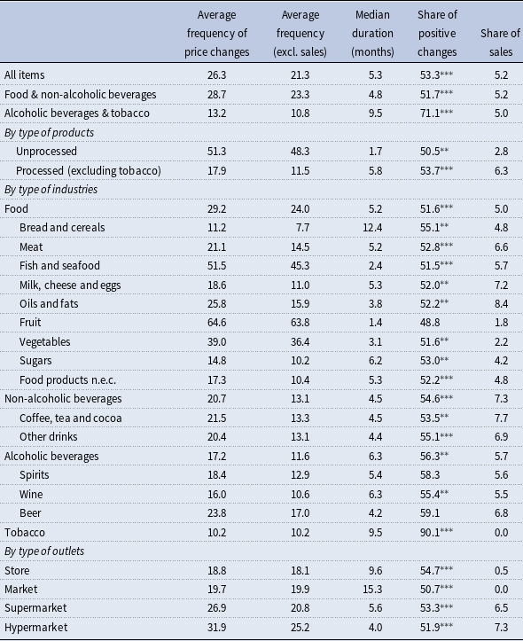
We identify four empirical facts about consumer price-setting behaviour in food products between January 2009 and December 2019. (1) We document that, in each month, about 1 out of 4 food items in the official CPI basket changed price compared with the month before. The average frequency of price changes was 26.3% when promotions and sales were included, and 21.3% when they were excluded. Upon closer examination, distinct patterns emerge across food categories and different retail formats: we have a striking difference between unprocessed (51.3%) and processed products (17.9%); at the outlet level, hypermarkets and supermarkets exhibited a higher frequency, reaching 31.9% and 26.9%, while markets and small stores had less frequent adjustments (19.7% and 18.8%, respectively). (2) The share of positive price changes on the total frequency of price changes was 53.3%, meaning that they were more frequent than the negative ones in this period. This holds across all subcategories, except for fruits, and when we exclude temporary price changes. The difference between positive and negative frequencies is statistically significant, suggesting asymmetric price adjustment behaviour. (3) We find that the positive adjustments exhibited a smaller magnitude compared to the negative changes. It is also worth noting that price changes were generally sizeable: the median change was 17.9%, regardless of its sign. (4) Finally, we report that price-setting behaviour was very heterogeneous not only across products but also at the industry and outlet level.
These regularities remain valid when we perform robustness checks: when we exclude extreme price changes; when we exclude promotions and sales using a sales filter instead of the sales flag provided in the dataset; and when we use the unit price to account for changes in product capacity. This analysis updates the evidence for Portugal provided by Dias et al. (Reference Dias, Dias and Neves2008). The authors used an analogous dataset on consumer prices for goods and services, allowing us to make comparisons over time. We also benchmark our findings within the context of the euro area.
We provide additional insights into the dynamics of price-setting behaviour over time. First, we document a stable path in the frequency of price changes, except for a temporary decline at the beginning of the sample period. This drop coincides with negative year-on-year inflation in food and non-alcoholic beverages. Despite this, if we exclude promotions and sales, we observe that the frequency of price changes has been trending downward over time: around 2009, it was above 25%, but by 2019 it had dropped to 20%. Second, we observe a marked increase in the size of price changes after 2012. This increase disappears when we drop temporary price changes from our sample. These two findings were driven by a shift in the pricing strategy among the industry’s main retailers: promotions shifted from occasional to the dominant pricing strategy.
Then, we assess how food inflation dynamics evolved over the business cycle. In Portugal, during the recovery from the Global Financial Crisis, negative inflation rates were associated with a lower share of positive price changes relative to negative ones. During the Sovereign Debt Crisis, inflation exceeded 2% and was driven mainly by more frequent upward adjustments in food prices, even though these adjustments were relatively small. Finally, during the expansion period from 2013 to 2019, inflation remained low and stable at around 0.5%, largely because downward price revisions exceeded upward ones. Then, a decomposition of month-on-month price variation reveals that inflation in this period was mainly driven by shifts in the relative frequency of positive versus negative price changes, rather than changes in their size.
Lastly, we examine other dimensions of food price-setting behaviour: producer prices were adjusted more frequently but with lower magnitude than consumer prices; and the comparison between monthly and daily data shows that the latter, with its higher temporal resolution, captures more frequent adjustments.
Beyond providing new micro evidence for Portugal, this study also speaks to the broader implications of food price-setting behaviour for inflation dynamics and macroeconomic modelling. The pronounced heterogeneity in pricing behaviour across industries and outlets shows that inflation responds not through a uniform adjustment of prices, but through shifts in the composition of firms that reprice in any given month. Our inflation decomposition further reveals that month-to-month inflation is driven mainly by changes in the frequency of price adjustments, consistent with models in which firms face menu costs or other frictions that limit the intensive margin of price changes. This pattern aligns well with the standard calibration of the New Keynesian model, where relatively infrequent but economically meaningful price revisions are sufficient to reproduce observed inflation behaviour. By documenting that these micro features hold for food prices, an essential, high-salience component of household consumption, we provide empirical support for this widely used calibration and highlight the importance of modelling heterogeneity and adjustment frequencies when evaluating the transmission of macroeconomic shocks and the effectiveness of monetary policy.
Related literature. Price stickiness remains a central question in macroeconomics because the understanding of price-setting behaviour and inflation dynamics helps to evaluate the transmission of monetary policy to the real economy. The theoretical foundation of price stickiness is significantly shaped by Ball and Mankiw (Reference Ball and Mankiw1995) and Taylor (Reference Taylor1999). These studies explore why prices do not adjust instantly to changes in economic conditions. Two primary models dominate this discourse: time-dependent models, as those in Taylor (Reference Taylor1980) and Calvo (Reference Calvo1983), posit that firms adjust prices at fixed intervals or with a fixed probability each period, respectively, making the timing of price adjustments exogenous; conversely, state-dependent models, such as those by Barro (Reference Barro1972) and Sheshinski and Weiss (Reference Sheshinski and Weiss1977), suggest that firms decide the timing and magnitude of price changes based on the state of the economy, thus treating these factors as endogenous variables.
More recently, empirical research has emerged in the literature and investigated the frequency and patterns of price adjustments across various markets and periods. Studies by Cecchetti (Reference Cecchetti1986), Kashyap (Reference Kashyap1995), and Lach and Tsiddon (Reference Lach and Tsiddon1992, Reference Lach and Tsiddon1996), among others, focused on small samples with a limited number of products, often revealing infrequent price changes. The seminal work by Bils and Klenow (Reference Bils and Klenow2004) expanded this scope by using a broader set of unpublished individual price data from the Bureau of Labour Statistics, which are used to calculate the US CPI, uncovering more frequent price changes and significant variation across products. Moreover, Nakamura and Steinsson (Reference Nakamura and Steinsson2008) established five facts about prices in the US that inspire our approach to describing price-setting behaviour in Portugal. We also provide evidence that is consistent with a benchmark menu-cost model.
The Eurosystem Inflation Persistence Network (IPN) extensively studied price stickiness in the euro area. This collaborative effort among national central banks and the ECB put together a vast array of datasets, including consumer and producer price indices and surveys on pricing behaviour.Footnote 1 The studies within the IPN, such as Fabiani et al. (Reference Fabiani, Druant, Hernando, Kwapil, Landau, Loupias, Martins, Mathä, Sabbatini, Stahl and Stokman2005) and Álvarez et al. (Reference Álvarez, Dhyne, Hoeberichts, Kwapil, Bihan, Lünnemann, Martins, Sabbatini, Stahl, Vermeulen and Vilmunen2006), provided comprehensive analyses of price stickiness across countries.Footnote 2 Dias et al. (Reference Dias, Dias and Neves2008) were the first to characterise the consumer price-setting behaviour in Portugal. They also used the data underlying the CPI, covering the period 1992–2001 and a wider range of goods and services. Despite the datasets used by the authors slightly differing from ours, the empirical features identified by the authors for the food products remain valid in our sample period. In our analysis, we show that the main facts are still qualitatively valid, but some differences emerge. We extend their results in two directions: first, we study price-setting behaviour over time and across the production value chain, and then we compare our monthly results with those obtained using daily data.
The Price-Setting Microdata Analysis research network continued this line of inquiry, further enhancing our knowledge of inflation dynamics. Gautier et al. (Reference Gautier, Karadi, Conflitti, Fabo, Fadejeva, Fuss, Kosma, Jouvanceau, Martins, Menz, Messner, Petroulas, Roldan-Blanco, Rumler, Santoro, Seward, De Veirman, Wieland, Wintr, Wursten, Zimmer, Amann, Faber, Bachiller and Stanga2023) documented five stylised facts about price adjustments in the euro area with low and stable inflation. Among other results, they find that for both consumer and producer prices, cross-sectoral heterogeneity is more pronounced than cross-country heterogeneity and that, consistent with idiosyncratic shocks as the main driver of price changes, aggregate disturbances affected inflation by shifting the relative number of firms increasing or decreasing prices, rather than the size of price increases and decreases. Recently, Gautier et al. (Reference Gautier, Conflitti, Faber, Fabo, Fadejeva, Jouvanceau, Menz, Messner, Petroulas, Roldan-Blanco, Rumler, Santoro, Wieland and Zimmer2024) also found a result consistent with ours for 11 other euro area countries: changes in the share of price increases among all changes matter more than movements in the size of price increases or decreases.
Outline. The paper is organised as follows. Section 2 describes the data and the methodology used. Section 3 presents the main facts on the consumer price-setting dynamics in food products. Sections 4 and 5 complement the analysis by describing price-setting behaviour over time and across other dimensions: the production value chain and a comparison with daily prices. Section 6 concludes.
2. Data and methodology
Consumer prices. We use a micro-level dataset on prices for the food products, collected by Statistics Portugal - Instituto Nacional de Estatística (INE). It includes granular information on two subindices, “Food and non-alcoholic beverages” and “Alcoholic beverages and tobacco,” used to construct the official aggregate CPI for Portugal and representing about 25% of the total consumption basket.
Within these subindices, we observe 394 products in different outlets over time. INE carefully selected the products to mirror the consumption habits of the resident population in Portugal, thus offering a representative snapshot of the consumer spending patterns over time.Footnote
3
We use an item, defined as a combination product
 $\times$
outlet, as the unit of observation. Then, we classify them by product type (unprocessed and processed), industry type (meat, fruit, vegetables, among others), and outlet type (store, market, supermarket, and hypermarket). In Table A.1, we present a complete set of the 5-digit ECOICOP (European Classification of Individual Consumption by Purpose) categories, in which items in our sample are classified. This is the most disaggregated level of detail that we are allowed to disclose. We also enumerate which ones are considered unprocessed and which are processed.
Our dataset consists of about 5.5 million price observations. The dataset spans from January 2009 to December 2019. It has a longitudinal setting: outlets are followed over time, on a monthly basis. The annual frequency distribution is described in Table A.2. More than 40,000 price quotes are collected every month from establishments across the country. Information on prices is collected through a statistical survey and reported at the product
 $\times$
outlet levels. INE ensures that all outlet types and regions are represented in the dataset, as shown in Tables A.3 and A.4. The variable of interest is the price of each item in a given month. We are thus able to compute descriptive statistics on the price-setting behaviour, focused primarily on two dimensions: frequency and magnitude.
In addition to prices, the dataset includes information on the outlet type, region, number of units per package, product capacity, product weight in the consumption basket, and a flag indicating promotions or sales. In the baseline analysis, we do not remove outliers, since they may reflect genuine episodes of sharp price adjustments that are relevant to studying price-setting behaviour. However, as a robustness check, we exclude extreme price changes by trimming observations, first, below the 1st and above the 99th percentiles of (log) price changes, and, second, below the 2nd and above the 98th percentiles. Given that product capacity may change over time, we also assess the robustness of our findings by using unit prices (i.e., price per unit of capacity) as the variable of interest.
Temporary price changes, such as promotions and sales, may play an important role in shaping the food price dynamics, as is commonly found in the literature. In our baseline analysis, we use effective prices, i.e., prices including discounts, as these correspond to the actual prices paid by consumers and are thus most relevant to the study of food inflation. Still, to better understand the role of discounts, a sales flag provided in the raw data is used to exclude items identified as being on sale. About 5.2% of price observations are identified as including promotions or sales, as reported in Table A.5. In Figure A.1, one can also observe that the frequency of sales was close to 1% from 2009 until 2013 and then increased substantially to more than 10% at the end of our sample period. Because the Statistical Office does not validate this variable, we also implement an alternative sales filter commonly applied in the literature by Nakamura and Steinsson (Reference Nakamura and Steinsson2008), with further details reported in Appendix B.1. The results using the sales filter serve as another robustness check.
The dataset used as a benchmark by Dias et al. (Reference Dias, Dias and Neves2008) differs in two key aspects. First, INE significantly increased the number of observed prices, which comes from the collection of prices for new products, additional varieties of the same products, and the change from quarterly to monthly price collection for most products. Moreover, there was an improvement in the country’s geographical coverage, which is also relevant to our analysis. This means that the current dataset is more representative of all establishments across the country and of households’ consumption structures. Nevertheless, it is important to note that this new series does not entail substantial methodological changes relative to the previous series.
Producer prices. We complement our study with two other micro-level datasets on food prices. First, we use producer prices in Section 5.1. This data is also collected by INE, and is intended to determine the monthly evolution of transaction prices in the national and external markets for a predetermined bundle of products, set by companies with some industrial activity. It is used to construct the aggregate Industrial Producer Prices Index (PPI) and spans the period from December 2010 to December 2019. This also includes a longitudinal setting with companies headquartered in national territory whose principal or secondary activity is mining and quarrying, manufacturing, and electricity, gas, and water supply, followed monthly over time. The unit of observation is an item, i.e., a product produced in a given establishment. Each item is classified using the Prodcom nomenclature at the 12-digit level (European Commission classification of industrial products) and matched at the most detailed level possible with items from the CPI dataset. For instance, one of the matches presented compares price changes in “Sugar” on the consumer side and “Manufacture of sugar” on the producer side. This yields a total of 26 matched categories, which are reported in Table A.6.
Daily prices. We also resort to supermarket daily prices (SDP), a dataset curated by Banco de Portugal Microdata Research Laboratory (BPLIM) (2024), in Section 5.2. This dataset includes daily prices from the online stores of the main Portuguese retailers. We focus on the period from September 2021 until the end of 2024.Footnote 4
Methodology. The frequency of price adjustments is defined as the fraction of times a price for an item in an outlet is changed over
 $T$
observation periods. We compute the frequency of price changes at the item level, using pairs of consecutive price observations within each store. We aggregate them at the monthly level, yielding a series of monthly price change frequencies. Since INE collects one price observation per month for each item, it may not capture price changes between two observations. Thus, our measures should be taken as lower bounds on the frequency of price changes. To see the relevance of this issue, we explore these intra-month price changes using daily price observations in Section 5.2.
The duration of price spells refers to the number of consecutive months in which the price level remains constant. We adopt the frequency approach for measuring price duration, as outlined by Bils and Klenow (Reference Bils and Klenow2004) and Dias et al. (Reference Dias, Dias and Neves2008): the average spell duration is calculated as the inverse of the frequency of price changes.
Finally, the CPI does not show the actual level of prices, but rather how prices have changed over time. As such, we analyse the magnitude of price adjustments as a simple log change, since consumer prices are displayed as indices.Footnote 5 Because averages are very sensitive to outliers and extreme values, we have opted to present the weighted median (as well as other quartiles) of the individual averages instead of the weighted average for the magnitude. Further details in Appendix B.3.
Sample period. Figure 1 shows the year-on-year rate of change for the headline index (solid line), the food and non-alcoholic beverages category (dashed), and the alcoholic beverages and tobacco category (dotted) from January 2009 to December 2019.
Consumer price index (CPI) over time.
Source: Statistics Portugal (INE).

During this period, overall inflation averaged 1% with a large standard deviation of 1.3%. There were periods of deflation between March and December of 2009, high-inflation above 3% in 2011 and 2012, and percentage changes very close to 0% for a long time from 2013 to 2017. The category of food and non-alcoholic beverages exhibited dynamics similar to the headline index, except during the deflationary periods in 2009 and 2014, when these products saw even more negative annual changes. For alcoholic beverages and tobacco, prices increased over the sample period, with an average yearly inflation of 3.7%. This underscores the relevance of this sample period, as it encompasses episodes of markedly different price dynamics, ranging from deflationary pressures to high-inflation episodes. Such heterogeneity is particularly interesting, as it allows us to assess the behaviour of price-setting under diverse macroeconomic conditions.
3. Consumer price-setting behaviour
This section explores the unpublished microdata underlying the official Portuguese CPI to document the main features of the consumer price-setting behaviour in food products. We highlight four main facts derived from the empirical analysis done and benchmark them against the results previously presented in similar studies. Each sheds light on the mechanisms that shape price dynamics in the Portuguese economy. We also present several robustness exercises we perform to ensure the reliability of our results: first, we exclude extreme price changes by trimming observations; then, we test with unit prices as the variable of interest; finally, we exclude promotions and sales using a sales filter.
Frequency of consumer price changes

Source: Authors’ calculations using disaggregated CPI monthly data.
Notes: The values correspond to the 2009:2 to 2019:12 period. The values use CPI weights at the most detailed level made available by INE, and the weights have been rescaled to add to one. The identification of temporary price changes uses the sales flag. The median duration is calculated as the inverse of the median frequency of price changes. A paired t-test is used to evaluate whether the mean difference between the frequency of positive and negative price changes is statistically significant (* p < 0.10, ** p < 0.05, *** p < 0.01). The number of observations and weights for each category are detailed in Table A.7. Sugars include sugar, jam, honey, chocolate, and confectionery. Other drinks include mineral waters, soft drinks, fruit, and vegetable juices. The price of tobacco is strongly influenced by taxation, so we exclude it from the processed products category.
3.1 Fact 1: In each month, about 1 out of 4 food items changed price
Table 1 reports the average frequency of price changes with and without temporary price changes in the sample, in the first and second columns. We compute these for all items together and for each type of product, industry, and outlet. The values are calculated using CPI weights at the most detailed level. The overall monthly frequency of price changes is 26.3%: in each month, about 1 out of every 4 food items in the official CPI basket had a different price than in the previous month. Moreover, the frequency of price changes excluding promotions and sales stood at 21.3%. Upon closer examination, distinct patterns emerge across categories.
Regarding the frequency of price changes by product type, we find a striking contrast between unprocessed and processed products: the former exhibit a frequency of 51.3%, whereas the latter show only 17.9%. Such pronounced volatility in unprocessed food prices underscores their inherent sensitivity to fluctuations in input costs, weather conditions impacting agricultural yields, and other supply-side shocks. Conversely, this pattern does not extend to processed food, which exhibited stronger rigidity. Similar conclusions hold when we remove temporary price changes.
These results indicate a marked decrease in the adjustment rhythms of food prices relative to those reported for the period 1997–2001 in Dias et al. (Reference Dias, Dias and Neves2008). The monthly frequency drops from 36.6% to 26.3%. This trend is specific to processed products, as prices for unprocessed products changed more frequently between 2009 and 2019. For the processed ones, we find that the frequency of price changes decreased from 23.9% to 17.9%.
We also benchmark our statistics against those of other euro area countries. Using the results from Gautier et al. (Reference Gautier, Conflitti, Faber, Fabo, Fadejeva, Jouvanceau, Menz, Messner, Petroulas, Roldan-Blanco, Rumler, Santoro, Wieland and Zimmer2024) as a comparison, food prices changed more frequently in Portugal than the average across the 11 countries analysed in this study. In the euro area, on average, 31.4% of unprocessed and 15.4% of processed changed every month.Footnote 6 We also confirm that excluding sales leads to a similar decrease in the frequency of price changes in this study: the size of the change is close to the share of sales in the dataset, which in our case was around 5.2%.
Distribution of the frequency of price changes by type of products.
Source: Authors’ calculations using disaggregated CPI monthly data.
Notes: The values correspond to the 2009:2 to 2019:12 period. Monthly averages were computed by item and constitute the basic observation. The distributions were obtained using kernel weights. No CPI weights were used. The price of tobacco is strongly affected by tax issues, so we exclude it from the processed category.

The distribution of frequencies of price changes by type of products, displayed in Figure 2, confirms that unprocessed products had a bi-modal distribution around 25% and 80%. This indicates that some products, such as fruits, had very frequent price changes (almost every month), whereas others, such as bread and cereals, milk, cheese, and eggs, changed less frequently. Regarding the processed ones, the distribution’s mass is more concentrated, with the right tail not exceeding 60% yet still exhibiting considerable within-group heterogeneity. These patterns are similar to those in Dias et al. (Reference Dias, Dias and Neves2008), with the only difference that the centre of mass of the distribution for the processed products is now around a lower level.
The third column of Table 1 shows the median spell durations, in months. We find that half of the items displayed price spells, which capture how long prices tend to remain unchanged, shorter than 5.3 months. The measured spells are longer for processed products (5.8 months) than for unprocessed ones (1.7 months). Notably, the highest median duration is observed in bread and cereals (12.4 months), whereas the shortest is observed in fruits (1.4 months). These findings show an increase in the median duration when compared to the period from 1997 to 2001, when it was around 3.1 months for food. This difference is mostly due to processed food, as the median duration increased from 5.3 months in the processed group and decreased from 2.1 months in the unprocessed group.
3.2 Fact 2: Positive price changes are more frequent than negative ones
Column 4 of Table 1 displays the share of positive price changes on total changes. Positive price changes were more frequent than negative ones, comprising 53.3% of all items in the sample. This also holds across all subcategories, except for fruits. The difference between frequencies is statistically significant at the 5% confidence level overall when we perform a paired t-test, indicating asymmetry in price adjustment behaviour.
As explained in Dias et al. (Reference Dias, Dias and Neves2008), these values close to each other may be a result of the seasonal nature of many items in this class, for which rises and drops in prices are expected to be equally likely. This is even more evident when filtering for unprocessed food, where the two values are 25.9% and 25.4% for positive and negative changes, respectively. Nevertheless, positive changes occur more systematically than negative ones over time, which might be influenced by the inflationary period under analysis. For the food category, year-on-year rates of change were primarily positive from 2009 until 2019, except for some months in 2009, 2010, and 2014. As expected in a context of positive but very low-inflation, the frequency of price increases surpassed that of price decreases. When we exclude temporary price changes from our sample, the share of positive changes increases to 54.6%, for all items, as shown in Table C.1. This increase is more pronounced in processed food and in supermarkets and hypermarkets, where sales are more prevalent.
These patterns can be benchmarked against the existing literature. Dias et al. (Reference Dias, Dias and Neves2008) also report that, despite operating in an inflationary environment, the monthly frequencies of price increases and decreases between February 1997 and January 2001 are very close, echoing our finding that the asymmetry, while not large in absolute terms, is nonetheless persistent. Evidence from the euro area in Gautier et al. (Reference Gautier, Conflitti, Faber, Fabo, Fadejeva, Jouvanceau, Menz, Messner, Petroulas, Roldan-Blanco, Rumler, Santoro, Wieland and Zimmer2024) reinforces this point: when sales are included, price increases account for about 54.5% of changes in unprocessed food and 57.0% in processed food. These magnitudes align closely with those we obtain. Their shares rise further once sales are excluded. Although ours also increase, the adjustment is more minor, suggesting that the underlying asymmetry is stable rather than mechanically driven by promotional activity. Similarly, Nakamura and Steinsson (Reference Nakamura and Steinsson2008) find comparable values for the United States between 1998 and 2005. Taken together, these studies show that a modest but systematic excess of price increases over decreases of the order we document is a common feature of food price-setting, even in low-inflation environments. In this sense, our results are consistent with the broader evidence, while adding a novel level of disaggregation by industry and outlet type.
An examination of these measures at the industry level indicates that positive price changes were more frequent than negative ones across all categories, with only one exception. Fruits recorded an average monthly frequency of price increases of 31.5%, while the share of items with price decreases stood at 33.1%. This reinforces the idea that prices in this subcategory were highly influenced by changes in market conditions, responding flexibly to supply-side changes related to their seasonal nature. The most significant discrepancy between the frequencies of positive and negative changes occurred in alcoholic beverages and tobacco, where positive changes accounted for 71% of total price changes (9.4% vs. 3.8%). The downward rigidity was particularly pronounced in tobacco, with a frequency of negative changes of only 1.0%, compared with 9.2% for positive changes.
A similar pattern emerges when prices are disaggregated by outlet type. Positive price changes systematically exceed negative ones in all outlet categories, and these differences are statistically significant. Stores exhibit the highest share of price increases (54.7%), followed by supermarkets (53.3%) and hypermarkets (51.9%). Markets are the closest to symmetry, with price increases representing 50.7% of monthly changes, yet even here, positive changes remain slightly more frequent. Taken together, these results confirm that the modest asymmetry in favour of price increases is a robust feature of retail food pricing.
3.3 Fact 3: Price increases have a smaller magnitude than price decreases
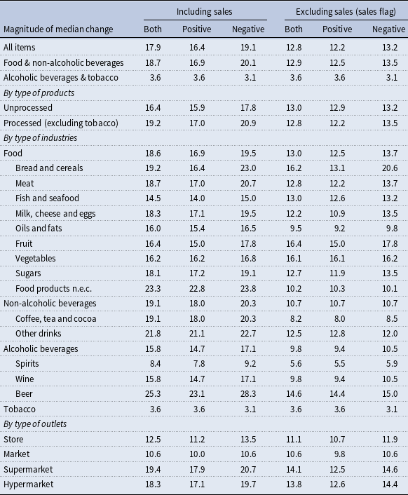
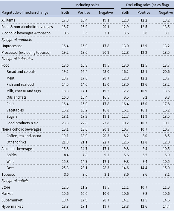
In Table 2, we characterise the magnitude of positive and negative price changes. The table reports the median (log) price changes conditional on a change having occurred (first and fourth columns), and on the sign of the change (remaining columns). It also shows the impact of excluding sales, using the sales flag.
Magnitude of consumer price changes
Source: Authors’ calculations using disaggregated CPI monthly data.
Notes: The values correspond to the 2009:2 to 2019:12 period. The values use CPI weights at the most detailed level made available by INE, and the weights have been rescaled to add to one. The identification of temporary price changes uses the sales flag. The number of observations and weights for each category are detailed in Table A.7. Sugars include sugar, jam, honey, chocolate, and confectionery. Other drinks include mineral waters, soft drinks, fruit, and vegetable juices. The price of tobacco is strongly influenced by taxation, so we exclude it from the processed products category.
The median size of a price change was 17.9%. Although price increases were more frequent, they tended to be smaller than price decreases. Positive price adjustments had a median magnitude of 16.4%, whereas negative ones had a median magnitude of −19.1%. This pattern holds when excluding sales: the median magnitude falls to 12.8%, and the difference between the absolute size of positive and negative changes narrows from 2.5% to 1%. The reduction in the median magnitude is driven primarily by the food and non-alcoholic beverages subcategory.
In contrast, the alcoholic beverages and tobacco category shows very small median magnitudes, around 3.6% for positive changes and −3.1% for negative ones, which remain essentially unchanged when excluding sales. This reflects, in particular, the pricing behaviour of the tobacco industry.
Moreover, excluding temporary price changes has a pronounced effect on supermarkets and hypermarkets, which rely more heavily on promotions and sales in their pricing strategies.
One can also confirm a clear difference between the distributions of the smaller stores and the larger retailers. While the magnitude of positive adjustments hovered around 11% for stores and 10% for markets, it was much higher for supermarkets (18%) and hypermarkets (17%). Similar patterns are observed in negative price movements. This will motivate the following empirical fact, in which we further disentangle heterogeneities in price-setting behaviour.
Compared with the euro area values in Gautier et al. (Reference Gautier, Conflitti, Faber, Fabo, Fadejeva, Jouvanceau, Menz, Messner, Petroulas, Roldan-Blanco, Rumler, Santoro, Wieland and Zimmer2024), we find that the magnitude of price changes was larger in Portugal for both processed and unprocessed foods. Despite this, they also found that the median decrease exceeded the median increase in both product categories. The comparison with the period 1997–2001 is not straightforward because Dias et al. (Reference Dias, Dias and Neves2008) used percentage changes. If we use percentage changes, as shown in Table C.2, we find an increase in the absolute size of price changes in both directions and that the interquartile ranges are narrower in both directions in our sample, with price changes more concentrated around the median.
In the Appendix, we present the distribution of price change magnitudes, conditional on the occurrence of a price change (i.e., zeros were excluded). Figure D.1 presents the distribution of the 25th, 50th, and 75th percentiles using all items in the sample. The median distribution is tightly concentrated around a small positive value, as most price changes were minor and positive. In contrast, the distributions for the 25th and 75th percentiles were more dispersed. This suggests a higher variability in price changes, with some items experiencing substantial decreases or increases. In the Appendix, we present the distributions for each percentile by product type (Figure D.2), industry (Figure D.3), and outlet (Figure D.4).
3.4 Fact 4: Price-setting behaviour is heterogeneous at industry and outlet level
Given the granularity of the data underlying the CPI consumer basket, it is possible to investigate the distribution of the frequency and magnitude of price changes across several dimensions. As such, we aim to understand the heterogeneity of price-setting behaviour across industries and outlets in the sample.
Figure 3 shows the distribution of the frequency of price changes for the main aggregates in Panel (a). Food and non-alcoholic beverages exhibited a multi-modal pattern with a long tail extending towards 100%. Despite this, the majority of price adjustments occurred at a frequency below 40%. This distribution is very close to the one obtained by combining all items, given the weight of this category. For alcoholic beverages and tobacco, the distribution is more concentrated around the median (10.5%), and 10% of items did not change in price. Within the food and non-alcoholic beverages category, on one hand, food and fish and seafood were the industries with the highest share of monthly price changes (64.6% and 51.5%, respectively). Vegetables also presented a high frequency. On the other hand, bread and cereals, sugar, jam, honey, chocolate, and confectionery had fewer price changes (11.2% and 14.8%, respectively).
Distribution of the frequency of price changes at industry and outlet level.
Source: Authors’ calculations using disaggregated CPI monthly data.
Notes: The values correspond to the 2009:2 to 2019:12 period. Monthly averages were computed by item and constitute the basic observation. The distributions were obtained using kernel weights. No CPI weights were used.

Figure 3 illustrates, in Panel (b), the distribution of price change frequencies for each type of outlet and shows that each one exhibits unique distribution patterns. Firstly, hypermarkets and supermarkets exhibited more frequent price fluctuations, as indicated by the denser, right-skewed density curves. In contrast, stores and markets exhibited greater concentration of low frequencies. In fact, hypermarkets stood out as the outlet type exhibiting the highest average frequency of price changes, at 31.9%. As the outlet size decreases, the values for each type also decrease: for the stores and markets, the frequencies are much lower (18.8% and 19.7%, respectively).
Additionally, a substantial percentage of items across all outlet types showed no price changes, reflecting segments of the distribution with zero frequency. This percentage is notably lower in the bigger outlets, consistent with their more volatile pricing behaviour. As a consequence, hypermarkets and supermarkets exhibited relatively shorter spells (4.0 and 5.6 months, respectively), whereas stores and markets demonstrated longer spells (9.6 and 15.3 months, respectively). This suggests that these smaller outlets tend to maintain consistent pricing over an extended period. The long tails in the distributions indicate that, although infrequent, item level price changes occurred across all outlets. Such findings may imply differences in pricing strategies, for example, fewer discounts, or unique market dynamics, potentially influencing consumer behaviour and competition. It may also come from higher menu costs for these outlets, which tend to be less efficient in frequently updating their prices.
The heterogeneity across categories is also corroborated by OLS regressions, in which we regress the average monthly frequency of price changes at the item level on product-, industry-, and outlet-type indicators, including time fixed effects. The results in Table C.3 confirm the substantial and systematic variation in price-setting behaviour across different segments of the CPI basket.
Robustness exercises. To ensure that our findings are robust across different settings, we repeat the computations of the frequency and magnitude statistics using different cleaning procedures for our sample that are common in the literature.
First, we exclude the extreme price changes by trimming observations as follows: (1) we exclude price changes below the 1st or above the 99th percentiles; and (2) we exclude price changes below the 2nd or above the 98th percentiles. Results are found in Tables C.4 and C.5 for the former and C.6 and C.7 for the latter. The empirical facts remain valid: the average frequency of price changes was close to one-quarter (25% in the first test and 23.8% in the second, for all items); positive changes were more frequent than negative ones (53.5% and 53.8%, respectively), but were smaller in magnitude. This shows that our main results are not driven by extreme price changes, but remain robust to alternative outlier-cleaning procedures. As such, we decided not to exclude any price changes in the baseline results, as the data is already subject to INE validation.
We also test using unit prices as the variable of interest, given that product capacity may change over time and imply a different unit price even though the regular price paid remains unchanged. We do not find any relevant changes in our results, as shown in Tables C.8 and C.9.
In the baseline exercise, we use the sales flag provided by INE, which is not used in the computation of official inflation statistics and therefore not subject to validation. As such, we consider an alternative approach to exclude temporary price changes: in Tables C.10 and C.11, we apply the sales filter proposed by Nakamura and Steinsson (Reference Nakamura and Steinsson2008) and employed by Gautier et al. (Reference Gautier, Conflitti, Faber, Fabo, Fadejeva, Jouvanceau, Menz, Messner, Petroulas, Roldan-Blanco, Rumler, Santoro, Wieland and Zimmer2024) to identify promotions and sales and then use it to exclude those from our sample. More details about how we exclude promotions and sales from our sample are available in Appendix B.1. One can see that the share of sales increases to 10.1%. This rise is mainly driven by unprocessed food at the product level, where the share of sales jumps from 2.8% to 13.9%. Given the sensitivity of these products to external factors, such a high share of sales may instead reflect very short-lived price changes that do not correspond to genuine promotions or sales. The sales filter, which identifies temporary price changes based on statistical criteria rather than directly on retailer-reported flags, might classify many of these short-lived adjustments as “sales.” At the outlet level, the share of sales also increases substantially for markets.
This approach results in a lower average frequency of price adjustments for all items: 21.3% with the sales flag and 16.9% with the sales filter, compared to 26.3% in the baseline. This pattern is consistent with the commonly documented effect in the literature that excluding temporary price changes reduces measured frequency. The median duration likewise increases, from 5.8 months in the baseline to 9.5 months (using the sales flag) and 10.9 months (using the sales filter), indicating that, once promotions and sales are excluded, prices remain unchanged for more extended periods. Despite these differences, the share of positive price changes remains very similar to that observed when sales are excluded using the sales flag. Regarding magnitudes, we find an additional interesting result: when discounts are excluded using the sales filter, median price increases exceed median price decreases. This is expected, as temporary discounts typically generate small and short-lived price reductions; once these are removed, the remaining adjustments mostly reflect regular upward revisions.
4. Price-setting behaviour over time
Price-setting decisions depend on factors that are not only specific to an individual firm or to the sector in which it operates (Dedola et al., Reference Dedola, Henkel, Höynck, Osbat and Santoro2024), but also on economy-wide disturbances. Aggregate shocks, such as recessions or deflationary episodes, and policy interventions, like tax reforms, can alter the incentives of many firms to adjust their prices. To understand their impact on inflation dynamics, it is essential to examine not just whether prices change, but also how they change. In particular, firms can respond along two distinct margins: the frequency of price adjustments, i.e., how often prices are changed, and the magnitude of those adjustments, i.e., how large the changes are when they occur. Analysing these two dimensions over time allows us to determine whether inflationary pressures arise primarily from more frequent price revisions or from larger individual price changes, thereby providing a clearer picture of how shocks propagate through firms’ pricing behaviour.
Frequency of price changes over time.
Source: Authors’ calculations using disaggregated CPI monthly data.
Notes: The values correspond to the 2009:2 to 2019:12 period. The values use CPI weights at the most detailed level made available by INE, and the weights have been rescaled to add to one. The identification of temporary price changes uses the sales flag. The vertical line in 2012:01 corresponds to a VAT change, and the one in 2017:02 corresponds to the introduction of a tax on sodas.

For the analysis in this Section, our baseline relies on the sample that excludes temporary price changes. We do so for two main reasons. First, from a theoretical standpoint, measures of price stickiness are more accurately captured when sales-related adjustments are removed, as such changes are typically less responsive to aggregate shocks. Second, the data exhibit a structural break in the frequency of sales, making it essential to verify that our results are robust to whether temporary price changes are included in the sample.
4.1 Frequency and magnitude of price changes over time
Figure 4 shows the evolution of the average frequency of price changes between 2009 and 2019. The black solid line shows the series excluding sales, and the grey one shows the series including sales. It also includes the evolution of the frequency of positive (dashed line) and negative (dotted line) price changes without sales.
The frequency of price changes has been trending downward over time: around 2009, it exceeded 25%, but by 2019 it had dropped to 20%. If we include temporary price changes, however, we see that it has evolved around its mean value, depending on the macroeconomic conditions that influence the inflation dynamics. In fact, during the first years of the sample, the fraction of items with price changes decreased. This decline coincides with negative year-on-year rates of change in food and non-alcoholic beverage prices. After 2012, it began increasing again toward the initial levels and remained near those levels by the end of the sample. This increase was mainly due to the increased use of promotions and sales as pricing strategies. The long-term stability around 25% reinforces the relevance of the stylised facts presented before, as these means capture the central tendency of firms’ pricing behaviour and provide a robust representation of the underlying patterns in price-setting. At the same time, the fluctuations around the mean suggest that the economic environment might be relevant to price-setting behaviour, motivating the analysis in the following subsection.
Changes in consumption tax rates can substantially affect the frequency of price adjustments (Bernardino et al. Reference Bernardino, Gabriel, Quelhas and Silva-Pereira2025). During our sample period, two major policy interventions generated pronounced shifts in the price-setting behaviour of a large number of items. The first occurred in January 2012, when most non-alcoholic beverages and a subset of food products experienced VAT rate changes: the rate increased from 6% to 23% for non-alcoholic beverages, while a restricted group of food items saw a reduction from 13% to 6%. These adjustments resulted in a sharp spike in the frequency of price changes, reaching nearly 70% for non-alcoholic beverages and over 30% for food items in that month. This spike is visible in the series for all items together around the first vertical line in Figure 4. A second intervention took place in February 2017 with the introduction of a soda tax, affecting part of the non-alcoholic beverages category (Gonçalves and Pereira dos Santos, Reference Gonçalves and dos Santos2020). This policy generated another pronounced but temporary increase in the frequency of price changes, which rose from around 20% to nearly 50% in a single month before returning to previous levels. By contrast, alcoholic beverages were not subject to any tax changes over the period, and their price adjustment frequency remained stable, with no significant deviations. This can also be seen around the second vertical line in the figure. These patterns are further illustrated in Figure D.5, which displays the evolution of price change frequencies by industry and clearly highlights the timing and impact of the two tax-related events.
A closer examination of the frequency of positive and negative price changes provides additional insights. As noted earlier, positive price changes were generally more frequent than negative ones, except during some months in 2009 and 2014, when year-on-year price changes were negative. Visual inspection also reveals how the gap between the two series evolved: in the early years, positive adjustments clearly dominated, whereas after 2014 the difference narrowed and was occasionally close to zero. In addition, positive price changes exhibited a pronounced seasonal pattern, particularly from 2009 to 2017, with peaks occurring in the early months of each year. This seasonality likely reflects items that undergo annual price revisions, consistent with the so-called “January effect.” Figure D.6 shows the monthly averages over the whole 2009–2019 period, confirming that aside from this early-year spike, there were no other meaningful seasonal variations. This means that the frequency of changes remained relatively stable across the rest of the year.
When examining the size of adjustments, Figure 5 provides a detailed view of the evolution of overall, positive, and negative price change magnitudes over the period, excluding promotions and sales. It also presents the series with the full sample in grey. A notable shift occurred in 2012, marking a significant change in the pattern of price adjustments. Before this shift, the magnitude of price changes was relatively stable, with adjustments averaging around 12%. During this period, positive price changes were consistently smaller than negative ones. However, starting in 2012, there is a marked increase in the median magnitude when temporary price changes are included. By 2017, it had escalated to approximately 22%.
Magnitude of price changes over time.
Source: Authors’ calculations using disaggregated CPI monthly data.
Notes: The values correspond to the 2009:2 to 2019:12 period. The values use CPI weights at the most detailed level made available by INE, and the weights have been rescaled to add to one. The identification of temporary price changes the sales flag. The vertical line in 2012:01 corresponds to a VAT change, and the one in 2017:02 corresponds to the introduction of a tax on sodas.

The increase in the gap between the frequency and the magnitude of price changes with and without sales after 2012 is closely related to a structural transformation of the Portuguese retail sector, which was concentrated in supermarkets and hypermarkets rather than in traditional stores and markets, as shown in Figure D.7. In May 2012, one of the largest retailers abandoned an Everyday Low Price (EDLP) strategy in favour of a High–Low (HILO) model, launching a “mega promotion” that marked a turning point in the industry’s pricing practices (Paixão, Reference Paixão2015). From then on, promotions shifted from occasional to the dominant pricing strategy, as competing retailers progressively adopted frequent, aggressive discounts to attract increasingly price-sensitive consumers in the aftermath of the financial crisis. This is the reason behind the structural break observed in the frequency of sales as reported in Section 2.
This transformation had significant implications for inflation dynamics. On the one hand, the reliance on promotions led to larger swings in shelf prices, thereby raising the short-term variability of measured inflation. On the other hand, the widespread use of discounts likely exerted downward pressure on underlying inflation by compressing margins and anchoring consumer expectations around promotional rather than regular prices. Importantly, when promotions and sales are excluded, the magnitude of price changes remains broadly stable over time, as shown in Figure 5, suggesting that the post-2012 increase in observed price volatility is primarily driven by the shift in promotional strategies in the modern retail sector. One can also note that there were no relevant seasonal effects over the year in the magnitude of price changes, as shown in Figure D.8.
4.2 The role of macroeconomic conditions
To evaluate if food inflation dynamics evolved differently over the business cycle, we distinguish three sub-periods within our sample: (1) the economic recovery from the Global Financial Crisis, spanning April 2009 to June 2010; (2) the recession associated with the Sovereign Debt Crisis, from July 2010 to March 2013; and (3) the long expansion phase from April 2013 until the onset of the Covid-19 pandemic in 2020. The definition of these periods follows the official recession dates fixed by the Business Cycle Dating Committee for Portugal (Aguiar-Conraria et al., Reference Aguiar-Conraria, Bação, Correia, Ferreira, Reis, Tavares, Valério and Varejão2023).
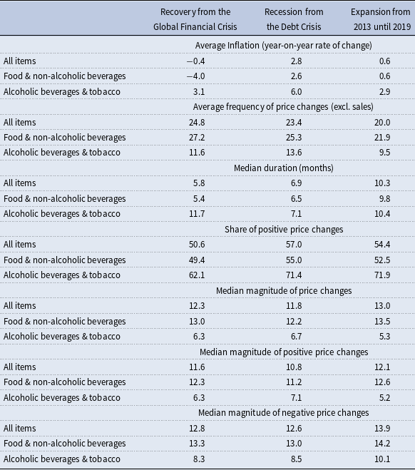
Frequency and magnitudes under different macroeconomic conditions
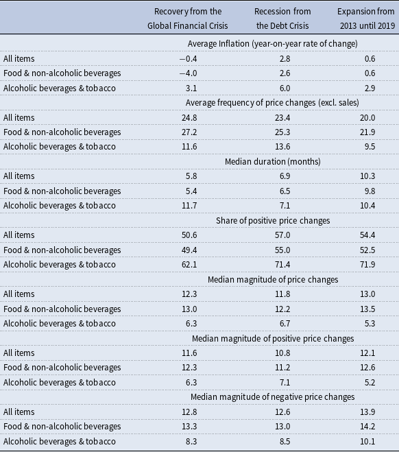
Source: Authors’ calculations using disaggregated CPI monthly data.
Notes: The values use CPI weights at the most detailed level made available by INE, and the weights have been rescaled to add to one. The magnitude values are conditional on a price change having occurred. We exclude temporary price changes to compute the frequency and magnitude statistics. The identification of temporary price changes uses the sales flag. The number of observations and weights are detailed in Table A.7.
During the recovery from the Global Financial Crisis, headline inflation averaged −0.4% and food prices declined at an average rate of −4.0%. In Table 3, we show that the frequency of price changes at high levels relative to other periods (24.8%), but the share of positive adjustments was relatively low (50.6%).Footnote 7 If we filter for the food and non-alcoholic beverages, this share is actually in favour of the negative changes (49.4%), consistent with the deflationary pressures in this category. The median size of both increases and decreases was modest (12.3%), with more substantial downward adjustments.
In the Sovereign Debt Crisis, headline inflation averaged 2.8%, supported in part by the alcoholic beverages and tobacco categories (average inflation of 6.0%). Food and non-alcoholic beverages registered positive, though more contained, inflation (2.6%). The frequency of price changes was lower than in the previous recovery phase, with an average of 23.4% across all items, and 25.3% for food products. The median duration increased, indicating that price adjustments were somewhat less short-lived. Significantly, the share of positive price changes increased markedly (57.0% overall, and 55.0% for food). The median size of price changes remained modest, at around 11.8% across all items, with a substantial decrease in the magnitude of positive price changes. Food price adjustments were in line with this average (12.2%), whereas changes in alcoholic beverages and tobacco were smaller (6.7%), suggesting more frequent but incremental revisions in these heavily taxed categories. Overall, the data reflect a period of positive, broad-based price pressures, with inflation driven primarily by frequent upward adjustments.
In the subsequent expansion phase, inflation moderated significantly, averaging 0.6% for food and overall, while remaining somewhat higher in alcohol beverages and tobacco (2.9%). The frequency of price changes decreased relative to the debt crisis, reaching 20.0% for all items and 21.9% for food products. The share of positive changes declined compared to the debt crisis, to 54.4% overall and 52.5% for food, consistent with subdued inflation. In alcohol and tobacco, however, upward changes still dominated (71.9%). The median magnitude of price changes rose considerably compared to earlier periods, reaching 12.1% across all items and 12.6% for food. The asymmetry between increases and decreases widened: downward revisions were, on average, larger (13.9%) than upward ones (12.1%). This pattern points to relatively infrequent but larger adjustments, a sign of greater nominal rigidity combined with larger shocks when firms did revise prices.
This business cycle analysis shows that both the frequency and the magnitude of price changes can vary across different macroeconomic environments. Yet, these statistics may conceal important dynamics that shape how inflation evolves month by month. To explore this, it is instructive to examine whether inflationary pressures are primarily associated with more firms adjusting their prices at a given point in time, or with larger individual adjustments once price changes occur. Conceptually, the distinction we explore in the following subsection matters because monthly inflation can be decomposed into the product of two components: the frequency of price changes and their magnitude. Analysing the relative contribution of each margin provides a clearer understanding of how shocks propagate through firms’ pricing behaviour and translate into aggregate inflation.
4.3 Decomposition of monthly inflation
A helpful way to understand the sources of inflation dynamics is to decompose monthly inflation into two underlying margins through which firms adjust prices: how often prices change (the frequency component) and by how much they change when they do (the magnitude component). The motivation for this decomposition is that these two margins reflect distinct economic mechanisms. Variations in the frequency of price changes are typically associated with changes in menu costs, information frictions, or firms’ responsiveness to macroeconomic conditions. In contrast, changes in the magnitude of price adjustments capture how firms revise their desired prices once they decide to reprice. By separating these components, we can assess whether inflationary pressures arise primarily because firms adjust prices more frequently or because they implement larger revisions conditional on repricing. This distinction is central for understanding the degree of price flexibility in the economy and, consequently, the transmission and effectiveness of monetary policy. This decomposition was first proposed by Klenow and Kryvtsov (Reference Klenow and Kryvtsov2008) and has since been widely applied, including in Gautier et al. (Reference Gautier, Conflitti, Faber, Fabo, Fadejeva, Jouvanceau, Menz, Messner, Petroulas, Roldan-Blanco, Rumler, Santoro, Wieland and Zimmer2024).
Formally, the standard decomposition expresses the month-on-month rate of inflation as the product of the fraction of prices that change and the average size of those changes. Denoting monthly inflation at month
 $t$
by
 $\pi _t$
, we write:
 \begin{equation} \pi _t = f_t \times dp_t, \end{equation}
where
 $f_t$
corresponds to the frequency of price changes and
 $dp_t$
to the magnitude.
Moreover, we can further decompose the frequency into the sum of the frequencies of price increases and price decreases, i.e.,
 $f = f^{+} + f^{-}$
. With this frequency decomposition, monthly inflation is obtained as the frequency of prices increases multiplied by the size of average price increases (
 $f^{+} \times dp^{+}$
) minus the frequency of price decreases multiplied by the (absolute) size of average price decreases (
 $f^{-} \times dp^{-}$
).
Next, we explore which component was more relevant for the inflation dynamics. We present the correlation between month-on-month inflation from January 2009 to December 2019 and the two components separately: first, the difference between the frequency of positive and negative price changes in Panel (a) of Figure 6; then, the difference between the size of positive and negative price changes in Panel (b).
Panel (a) shows a strong positive correlation between monthly inflation and the frequency component, indicating that variations in the frequency of positive versus negative price changes significantly affect monthly inflation. In contrast, Panel (b) reveals no correlation between inflation and the magnitude component, suggesting that the size of price adjustments had little impact on the inflation dynamics. These results indicate that inflation during this period was primarily driven by the relative frequency of positive versus negative price changes, rather than by changes in price magnitudes. Specifically, when the frequency of positive price changes exceeded that of negative changes, inflation tended to rise significantly. By contrast, the magnitude of price adjustments appeared to play a limited role, as its correlation with monthly inflation was close to zero. Consequently, pricing strategy shifts that primarily alter the size of adjustments, without affecting how often firms reprice, are unlikely to influence month-to-month inflation significantly. From an inflation-monitoring perspective, such developments thus warrant limited concern.
Correlation between monthly inflation and frequency or magnitude components.
Source: Authors’ calculations using disaggregated CPI monthly data.
Notes: The values correspond to the 2009:2 to 2019:12 period. Each dot represents a month. The CPI weights were used at the most detailed level available. We exclude temporary price changes to compute the frequency and magnitude statistics. The identification of temporary price changes uses the sales flag.

This shows that, when inflation is high, firms tend to adjust their prices more frequently, thus increasing price flexibility. As such, for the conduct of monetary policy, the frequency component constitutes the more relevant dimension to monitor. Moreover, greater flexibility lowers the economic cost of reducing inflation, making it easier for central banks to bring inflation down without causing significant losses in output or employment and to achieve a “soft landing.” In these circumstances, monetary policy can be more aggressive in addressing inflation because the trade-off between disinflation and economic activity is less severe (Karadi et al., Reference Karadi, Nakov, Nuño, Pasten and Thaler2025). Similar results have been found for other countries, such as the euro area (Gautier et al., Reference Gautier, Conflitti, Enderle, Fadejeva, Grimaud, Gutiérrez, Jouvanceau, Menz, Paulus, Petroulas, Roldan-Blanco and Wieland2025), the US (Nakamura et al., Reference Nakamura, Steinsson, Sun and Villar2018; Karadi et al., Reference Karadi, Amann, Bachiller, Seiler and W.2023), the United Kingdom (Hahn and Marenčák, Reference Hahn and Marenčák2020), and Sweden (Ewertzh et al., Reference Ewertzh, Klein and Tysklind2022).
5. Other dimensions of food price-setting behaviour
5.1 Price-setting behaviour over the production value chain
We complement the analysis of consumer prices with industrial producer prices to explore how price-setting behaviour changes over the production value chain. We match the categories from CPI and PPI datasets at the most detailed level possible, yielding a total of 26 categories.Footnote
8
Figure 7 compares the average frequency of price changes at the consumer (excluding promotions and sales) and producer levels for each one of the categories matched, controlling for its direction. The 45
 $^{\circ }$
line indicates that the frequency is the same for a specific category. If the point lies above (below), then the frequency is lower (higher) at the consumer level.
Frequency of price changes at the consumer and producer levels.
Source: Authors’ calculations using disaggregated CPI and PPI monthly data.
Notes: The values correspond to the 2011:1 to 2019:12 period. The items were matched at the most detailed level. Each dot corresponds to a match. No CPI weights were used. We exclude temporary price changes to compute the frequency statistics. The identification of temporary price changes uses the sales flag.

Our findings reveal a higher frequency of price changes at the producer level than at the consumer level. This result holds for both positive and negative price changes. In Figure D.9, we show this without controlling for the direction. The relatively low correlation between the frequency of price changes for CPI and PPI (18.5% for positive changes and 26.1% for negative changes) suggests that price transmission along the production-consumption chain is far from perfect.
An important reason is that the purchase of goods constitutes only one part of retailers’ total costs, with other components, such as wages and rents, being generally more stable. As a result, consumer prices do not move as much as producer prices, even if producers pass on all their cost changes directly. Firms can also use their profit margins to smooth fluctuations in purchasing costs, absorbing normal variations without adjusting retail prices. In cases where purchasing prices rise faster than usual, companies may allow margins to fall temporarily and adjust them again later, avoiding frequent price changes for competitive reasons or to minimise menu costs. Another factor is that a substantial share of consumer goods is imported rather than domestically produced. As such, changes in PPI affect only part of the CPI basket, limiting the extent to which producer price movements translate into consumer prices. These considerations highlight the importance of supply chain dynamics and intermediary processes in shaping observed pricing patterns, suggesting that producer price movements are not mechanically or immediately reflected in consumer prices, even for matched product categories.
Looking at the median magnitudes of the variation in prices in Figure 8, we find that they are larger at the consumer level. Interestingly, the size of price changes for industrial producers tends to be very low and concentrated, both for positive and negative changes. There is thus a contrast over the production value chain: producer prices change more frequently but by less than consumer prices.
Median magnitudes of price changes at the consumer and producer levels.
Source: Authors’ calculations using disaggregated CPI and PPI monthly data.
Notes: The values correspond to the 2011:1 to 2019:12 period. The items were matched at the most detailed level. Each dot corresponds to a match. No CPI weights were used. We exclude temporary price changes to compute the frequency statistics. The identification of temporary price changes uses the sales flag.

5.2 Comparison against daily prices
To construct the CPI, one price observation is collected per month for each item. As such, the measures of the frequency and magnitude of price changes obtained from the CPI dataset should be interpreted as lower bounds, since intra-month adjustments may not be captured. In this context, we conclude our analysis of consumer price-setting behaviour by comparing it with the daily online prices. The goal is to understand whether the frequency and the magnitude of price changes differ significantly between the two datasets: the one collected by INE (CPI) and the one with daily supermarket data (SDP).Footnote 9 Further details are reported in Appendix B.2. Figure D.10 presents comparisons of frequency and magnitude statistics computed using monthly and daily data in the Appendix.
The findings indicate that the frequency of price changes is generally higher in the daily SDP data across most categories. This discrepancy can be attributed to the higher temporal resolution of the SDP dataset, which captures more granular price movements that the monthly CPI data may miss. Temporary promotions, flash sales, or other intra-month adjustments are likely to be reflected in the SDP data but remain undetected in the CPI data even when excluding them for temporary price changes. This confirms that these statistics most certainly under-report the true frequency of price changes, thereby affirming the hypothesis that these values should be treated as lower bounds. As expected, the size of price changes appears to be higher in the CPI data. As the CPI reflects a single monthly price, it is more likely to record significant changes when they occur, potentially skewing the magnitude upwards compared to the daily dataset, where more minor but more frequent adjustments might dilute the average magnitude.
6. Conclusion
Price stickiness remains a core question, with new micro evidence playing a central role in further deepening its understanding. This paper leverages a novel dataset of official CPI microdata for food products in Portugal between 2009 and 2019, thereby expanding the evidence on the dynamics of food prices.
First, we document four main features of the consumer price-setting behaviour. Our analysis reveals that over one-quarter of food prices changed each month during the study period. Notably, there are distinct patterns across food categories and retail formats. Unprocessed products showed a higher frequency of price changes, with 50% of items adjusting prices monthly, compared to only 18% for processed food. Hypermarkets and supermarkets reported the highest frequency of adjustments, while smaller stores and markets reported fewer. Positive price changes occurred more often than negative ones but tended to be smaller in magnitude. The magnitude of these changes is generally substantial, usually exceeding average inflation for the period.
We also show that aggregate shocks, such as recessions and deflationary episodes, or policy interventions, such as tax reforms, can alter the incentives of many firms to adjust their prices. By decomposing month-to-month rates of change, we conclude that differences in the frequency of price changes largely explained inflation in this period, with increases relative to decreases, rather than by changes in the average size of adjustments. A comparison of producer and consumer price levels shows that while producer prices changed more often, the magnitude of these changes was smaller than the larger but less frequent price adjustments observed at the consumer level. Finally, using daily price data points towards a higher true frequency of price changes, but smaller magnitude statistics, capturing more granular price movements that the monthly CPI data may miss.
Supplementary material
The supplementary material for this article can be found at https://doi.org/10.1017/S1365100526100844.
Acknowledgements
This paper was produced in the context of the Price-Setting Microdata Analysis (PRISMA) research network. We thank Statistics Portugal (INE) for access to the data. We are grateful to Vítor Mendonça, Álvaro Silva, Margarida Rosa, Adelina Andrade, Idílio Freire, and Elsa Silva from INE for the important help regarding methodological aspects of the microdata used in this project. We thank Domingos Seward for the excellent assistance on the analysis of the microdata, Lucena Vieira, Ana Catarina Pimenta, Sónia Félix, Catherine Fuss, Daniel Dias, Pedro Duarte Neves, Nuno Lourenço, Tiago Bernardino, Ricardo Gonçalves, Erwan Gautier, Gabriel Z’ullig, and Alberto Cavallo for comments and suggestions. The views expressed herein represent the views of the authors and not necessarily those of the Banco de Portugal or the Eurosystem. Any errors or omissions are the sole responsibility of the authors.
Funding statement
This work was supported by the FCT (Fundação para a Ciência e a Tecnologia) [grant number UIDB/05069/2020].
Competing interests
The authors declare none.