


I. INTRODUCTION
Wireless Power Transfer (WPT) based on resonant inductive coupling has recently gained great interest among researchers, representing an attractive solution for wirelessly powering electronic devices and systems [Reference Hanazawa and Ohira1–Reference Costanzo6]. The basic implementation consists of two magnetically coupled inductors with series or shunt capacitors realizing the resonant condition at the operating frequency of the link. As numerically and experimentally demonstrated in a large number of works [Reference Kurs, Karalis, Moffatt, Joannopoulos, Fisher and Soljacic7–Reference Dionigi and Mongiardo13], with respect to a simple inductive coupling, the use of resonant schemes allows improving the performance and the sensitivity of the link with regard to the operating conditions (alignment, operating environment, etc.). However, for a given resonant scheme, an appropriate design is necessary in order to achieve optimal performance in a specific application. In particular, in some applications the focus is in providing to a given load the power necessary for the correct operation (see the case of medical implants [Reference Monti, Arcuti and Tarricone5]), while in some others the focus is on the efficiency of the link (see the case of vehicular applications [Reference de Santiago14, Reference Haghbin, Lundmark, Alakula and Carlson15]).
In this regard, useful design formulas have been presented in [Reference Dionigi, Mongiardo and Perfetti16, Reference Monti17], where, for a given two-port network representing a single transmitter-single receiver WPT link, closed form formulas for the load realizing different approaches of interest for practical applications have been derived.
In particular, in [Reference Dionigi, Mongiardo and Perfetti16], the problem of efficiency and power maximization has been solved demonstrating that different loads are necessary for the two approaches. Additionally, by using the conjugate image impedances of the network, the solution realizing the complex conjugate matching for the assigned network has been also determined.
However, although the problem of determining the optimal terminating impedances for a given WPT link has been exhaustively analyzed and solved, the inverse problem, which is of interest in many applications [Reference Costanzo, Dionigi, Mongiardo, Monti and Perfetti18], has not yet been comprehensively addressed: are not currently available in the literature the general formulas for maximizing the power and/or the efficiency of a generic inductive WPT link with respect to assigned values of the terminating impedances. Accordingly, in this paper a WPT link represented as a two-port network is considered, and the problem of determining the optimal design for given values of the network input and load impedances is solved. With respect to the analysis presented in [Reference Costanzo, Dionigi, Mongiardo, Monti and Perfetti18], where the case of a resonant inductive WPT link using two series resonators was considered, more results and discussions are provided in this paper by solving the general case where the link can be realized by using series or parallel resonators. For the four possible schemes (Parallel-Parallel (PP), Series-Series (SS), Parallel-Series (PS), and Series-Parallel (SP)), closed form analytical formulas for the network parameters realizing the optimal design are derived and discussed. It is demonstrated that there is just one optimal design of the two–port network that simultaneously allows maximizing the two main figures of merit of interest (i.e., the power on the load and the power transfer efficiency of the link).
The paper is structured as follows. In Section II the optimal design is derived for the general case of a resonant WPT link with given values of the input and load impedances, in Sections III and IV the theory is applied to the case of WPT link using a resonator with a parallel arrangement on port 1 and a resonator with a series arrangement on port 2. In Section V, closed form formulas are provided for the parameters realizing the optimal design in the cases of a PP, SS, and a SP configuration. Finally, circuital simulations are reported in Section VI and some conclusions are drawn in Section VII.
II. DESIGN OF A WPT LINK BASED ON RESONANT INDUCTIVE COUPLING: GENERAL CASE
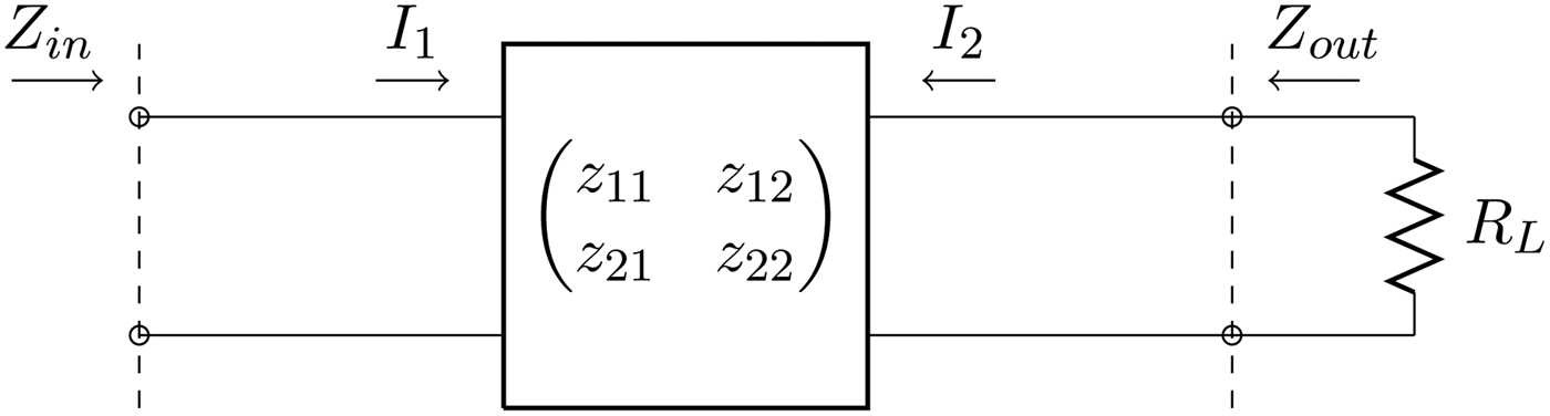
The problem considered in this paper is illustrated in Fig. 1. Let us consider two coupled inductances L 1 and L 2 with series or parallel capacitances C 1 and C 2 realizing the resonance condition at the operating frequency of the link ω 0, i.e.:
 $$\omega _0 = \displaystyle{1 \over {\sqrt {L_1C_1} }} = \displaystyle{1 \over {\sqrt {L_2C_2} }}. $$
As illustrated in Fig. 1, the WPT link can be modeled as a reciprocal two-port network (i.e., z 12 = z 21), represented by its impedance matrix, with elements z ij = r ij + jx ij , with i, j = 1, 2, given as:
 $$V_1 = z_{11}I_1 + z_{12}I_2,$$
 $$V_2 = z_{12}I_1 + z_{22}I_2. $$
It is assumed that the link is driven by a sinusoidal voltage generator
 $v_G(t) = V_G\cos (\omega t)$
with internal resistance R
G
, and that the output port of the link is connected to a given load resistance R
L
. It is also assumed that the generator requires, for optimal operation, to be connected to a given load resistance R
o
. This condition encompasses a wide range of practical cases, including, for instance, the case where the generator represents a power amplifier designed for providing maximum efficiency when loaded by R
o
, or the case where it is required to maximize the power delivered by the generator, and, consequently, the load resistance R
o
has to be equal to R
G
. Hence the term optimal may have different meaning depending upon the specific application. Accordingly, our goal is to design the network in such a way that its input impedance is
 $$Z_{in} = R_o, $$
and it provides optimal performance when loaded by R L .
Schematic representation of the problem is analyzed in this paper. A reciprocal two-port network represented by its impedance matrix Z is considered. The goal is determining the network parameters realizing the optimal design for given values of the input impedance Z in and of the load resistance R L .

With reference to the use of a two-port network for realizing a WPT link, in general, two different solutions are of interest [Reference Dionigi, Mongiardo and Perfetti16, Reference Monti17], namely the Maximum Power Delivered to the Load (MPDL) solution, where the goal is maximizing the active power delivered to the load (
 $P_L = (1/2)R_L\left\vert {I_L} \right\vert^2$
), and the Maximum Power Transfer (MPTE) solution, where the goal is maximizing the efficiency of the link defined as [Reference Bird, Rypkema and Smart19, Reference Zargham and Gulak20]:
 $$\eta = \displaystyle{{P_L} \over {P_{in}}}.$$
The quantity P in which appears in (5) is the active input power delivered to the two-port network by the voltage generator:
 $$P_{in} = \displaystyle{1 \over 2}\displaystyle{{R_{in}} \over {{\left \vert {Z_{in}} \right \vert} ^2}}V_1^2, $$
where V 1 is the voltage at the input port of the link, while Z in = R in + jX in is the input impedance of the network seen by the generator. It can be noted that if Z in is fixed, as in the present case, the input power P in that can be delivered to the network by the generator is also fixed. Consequently, from (5) it can be easily derived that maximizing the power transfer efficiency also corresponds to maximizing the power delivered to the load. Hence, in this case there is just one optimal design that realizes both the MPTE and the MPDL solutions.
In [Reference Dionigi, Mongiardo and Perfetti16] it is shown that for a reciprocal two-port network loaded by a purely resistive impedance and operating in MPTE condition, the input and the load resistance coincide with the conjugate image impedances.
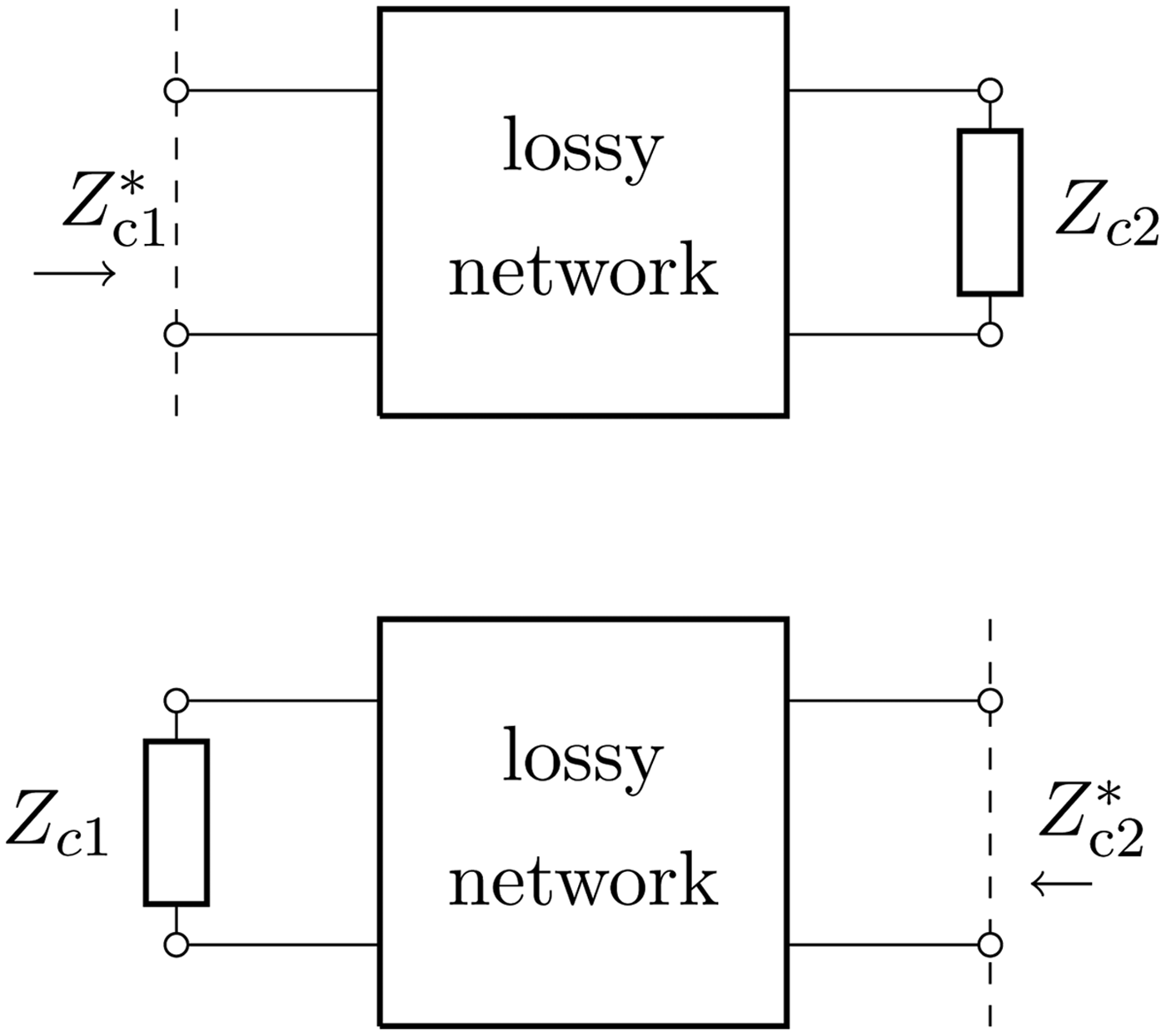
The conjugate image impedances [Reference Roberts21, Reference Inagaki22] are an intrinsic property of the network defined as illustrated in Fig. 2, and can be computed as described in [Reference Roberts21]. By recalling the results reported in [Reference Roberts21], the steps required for determining the expressions of the conjugate image impedances of a two-port network represented by its impedance matrix are summarized in the following part of this section.
Conjugate image impedances as defined in [Reference Roberts21] (see Fig. 3 of [Reference Roberts21]). Upper figure: when port 2 is terminated on Z
c2 the input impedance seen from port 1 is
 $Z_{c1}^* $
(the asterisk denotes the complex conjugate). Similarly, in the lower figure, when port 1 is terminated on Z
c1 the input impedance seen from port 2 is
 $Z_{c2}^* $
.

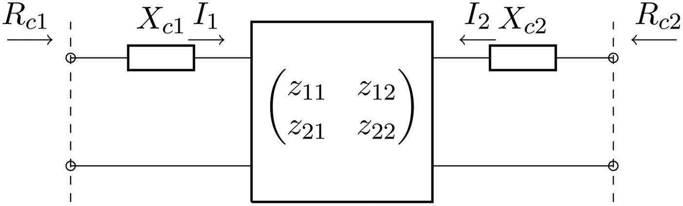
Schematic representation of a two-port network described by its impedance matrix Z with compensating reactances on port 1 and 2. It is assumed that the conjugate image impedances of the network are Z c1 = R c1 + jX c1 and Z c2 = R c2 + jX c2. By adding the compensating reactance X c1 on port 1 and X c2 on port 2, we obtain a network that, when terminated on the resistive impedance R c2, presents a resistive input impedance R c1.

Referring to the two-port network shown in Fig. 1, it is convenient to define the parameters:
 $$\chi ^2 = \displaystyle{{x_{12}^2} \over {r_{11}r_{22}}},$$
 $$\xi ^2 = \displaystyle{{r_{12}^2} \over {r_{11}r_{22}}}, $$
and to introduce the following definitions:
 $$\theta _r = \sqrt {1 + \chi ^2} \sqrt {1 - \xi ^2}, $$
 $$\theta _x = \chi \xi . $$
With these positions, the conjugate image impedances Z ci can be expressed as (see equation (6b) of [Reference Roberts21]):
 $$Z_{c1} = R_{c1} + jX_{c1} = r_{11}(\theta _r + j\theta _x) - jx_{11},$$
 $$Z_{c2} = R_{c2} + jX_{c2} = r_{22}(\theta _r + j\theta _x) - jx_{22}.$$
In order to design a link with input impedance equal to R o , and providing, when loaded by a resistance R L , maximum power transfer efficiency, which in the present case also implies maximum power to the load, the following conditions must be imposed:
 $$\eqalign{& Z_{c1} = R_o, \cr & Z_{c2} = R_L.} $$
According to (13), purely resistive values of the conjugate image impedances have to be realized. From Fig. 2 and by using the expressions (11) and (12), it is evident that this requires to add two series compensating reactances X c1 and X c2 as shown in Fig. 3:
 $$X_{c1} = r_{11}\theta _x - x_{11},$$
 $$X_{c2} = r_{22}\theta _x - x_{22}.$$
Once the compensating reactances have been added to the network, the optimal design can be realized by setting the network parameters according to the following relations:
 $$R_{c1} = r_{11}\theta _r = R_o,$$
 $$R_{c2} = r_{22}\theta _r = R_L.$$
In the following sections, these equations will be used for calculating the values of the inductances of a resonant inductive link realizing the optimal design. Starting from the case where the resonator on port 1 has a parallel configuration, and the resonator on port 2 has a series configuration, different schemes will be analyzed and discussed.
III. OPTIMAL DESIGN OF A WPT LINK USING A PARALLEL RESONATOR MAGNETICALLY COUPLED WITH A SERIES RESONATOR
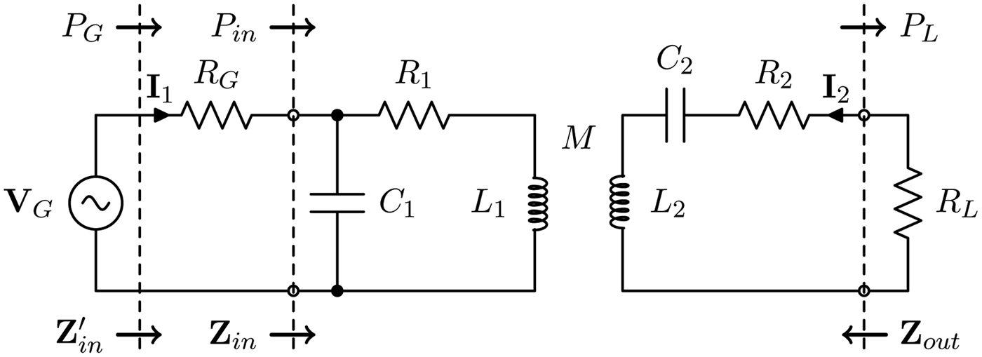
In this section, the theory developed in the previous part of the paper will be applied to the resonant WPT link illustrated in Fig. 4 and consisting of two coupled inductances with compensating capacitances; as it can be seen from Fig. 4, a parallel configuration is assumed on the primary side, while a series arrangement is assumed on the secondary side. In the following part of the paper this configuration will be referred as a PS configuration. It is assumed that the link is driven by a sinusoidal voltage generator
 $v_G(t) = V_G\cos (\omega t)$
with internal resistance R
G
and that the output port of the link is connected to a resistive load R
L
.
Schematic of a WPT link using a resonator with a parallel arrangement on the primary side and a resonator with a series arrangement on the secondary side.

The resistors R 1 and R 2 represent the inductor losses and are related to the inductor quality factors Q i , (i = 1,2) by the following relation:
 $$R_i = \displaystyle{{\omega _0L_i} \over {Q_i}}.$$
It is also convenient to introduce the coupling coefficient
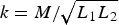 $k = M/\sqrt {L_1L_2} $
, the transform ratio
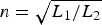 $n = \sqrt {L_1/L_2} $
, and the reactance slope parameter of the primary resonator
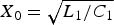 $X_0 = \sqrt {L_1/C_1} $
.
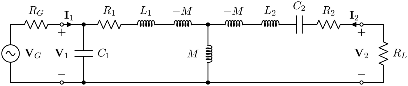
It can be noted that the link can be represented by the equivalent circuit of Fig. 5, where the T-network formed by the inductances -M, M and -M act as an immittance inverter.
Equivalent circuit of the WPT link.

According to the theory developed in the previous section, our goal is to determine the value of the inductances for which R in = R o and the power transfer efficiency is maximum when the network is loaded by a given R L .
A) Impedance matrix computation
In order to apply to the PS configuration of Fig. 4 the theory presented in Section II, we need to determine the impedance matrix of the network. To this end it is convenient to compute its ABCD transmission matrix which can be expressed as the product of the matrices T 1, T i , T 2:
 $$T = T_1 T_i T_2$$
where T
1 refers to the shunt capacitor C
1, the series R
1, and the series L
1, T
i
is the the ABCD matrix of the immittance inverter, while T
2 refers to the series L
2 with its associated resistance, and the series capacitor C
2. Assuming that the network is operating at its main resonant frequency, the following expression can be derived for
 $T_1 T_i T_2$
:
 $$T_1 = \left( {\matrix{ 1 & {\displaystyle{{X_0} \over {Q_1}} + j X_0} \cr {\displaystyle{j \over {X_0}}} & {\displaystyle{j \over {Q_1}}} \cr}} \right),$$
 $$T_i = \left( {\matrix{ 0 & { - \displaystyle{{j X_0 k} \over n}} \cr { - \displaystyle{{j n} \over {k X_0}}} & 0 \cr}} \right),$$
 $$T_2 = \left( {\matrix{ 1 & {\displaystyle{{X_0} \over {Q_2 n^2}}} \cr 0 & 1 \cr}} \right).$$
Accordingly, for the total transmission matrix T we obtain:
 $$T = \left( {\matrix{ { - \displaystyle{{j n - Q_1 n} \over {Q_1 k}}} & { - \displaystyle{{j \left( {Q_1 Q_2 k^2 + 1} \right) X_0 - Q_1 X_0} \over {Q_1 Q_2 k n}}} \cr {\displaystyle{n \over {Q_1 k X_0}}} & {\displaystyle{{Q_1 Q_2 k^2 + 1} \over {Q_1 Q_2 k n}}} \cr}} \right).$$
From (23), it can be derived that the impedance matrix has the following expression:
 $$Z_{ps} = \left( {\matrix{ {Q_1 - j} & {\displaystyle{{Q_1 k} \over n}} \cr {\displaystyle{{Q_1 k} \over n}} & {\displaystyle{{Q_1 Q_2 k^2 + 1} \over {Q_2 n^2}}} \cr}} \right)X_0.$$
B) Optimal design of the PS configuration: network parameters determination
In the case of a PS configuration, the parameters defined in (10) for the general case are:
 $$\theta _r = \displaystyle{1 \over {\sqrt {Q_1 Q_2 k^2 + 1}}}, $$
 $$\theta _x = 0.$$
The conjugate image impedances are readily obtained
 $$Z_{c1,ps} = (Q_1\theta _r + j)\,X_0,$$
 $$Z_{c2,ps} = \left( {\displaystyle{1 \over {\theta _r Q_2 n^2}}} \right) X_0.$$
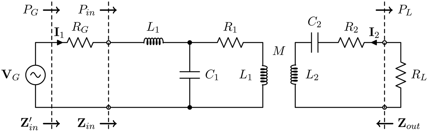
In order to realize resistive values for the conjugate image impedances, from (27) and (28) it is apparent that we need to insert an additional inductance of the same value of L 1 (i.e., X c1,ps = ωL 1) on the primary side, while no modification is necessary on the secondary side (i.e., no compensating reactance is necessary on port 2). Accordingly, the network becomes the one illustrated in Fig. 6 and the optimal design can be realized by using (16) and (17) for setting the values of the inductances L 1, L 2.
A series inductance L 1 has been added on the primary side in order to realize a real conjugate image impedance.

To this end, it is convenient first to compute the conjugate image impedances as
 $$R_{c1,ps} = Q_1\theta _r\omega _0L_1,$$
 $$R_{c2,ps} = \displaystyle{{\omega _0L_1} \over {\theta _r Q_2 n^2}}.$$
Then, by imposing that
 $$R_{c1,ps} = R_o,$$
 $$R_{c2,ps} = R_L,$$
it is possible to recover the values of the inductances realizing the optimal design:
 $$L_{1,ps} = \displaystyle{{R_o} \over {\omega _0 Q_1\theta _r}},$$
 $$L_{2,ps} = \displaystyle{{Q_2 R_L\theta _r} \over {\omega _0}}.$$
IV. PS CONFIGURATION: ANALYSIS OF THE PERFORMANCE
Let us consider a real impedance matrix, as obtained e.g. for the PS configuration when the compensating reactances X c1 and X c2 have been added in series to port 1 and port 2. When considering a 1 V (peak amplitude value) voltage generator connected to port 1, we have the following two equations for the currents:
 $$1 = I_1\;(R_G + r_{11}) + I_2 r_{12},$$
 $$0 = I_2\;(R_L + r_{22}) + I_1 r_{12}$$
with solutions
 $$I_1 = \displaystyle{{R_L + r_{22}} \over {(R_G + r_{11}) (R_L + r_{22}) - r_{12}^2}},$$
 $$I_2 = - \displaystyle{{r_{12}} \over {(R_G + r_{11}) (R_L + r_{22}) - r_{12}^2}}.$$
Accordingly, the input resistances
 ${R}^{\prime}_{in} = 1/I_1$
and
 $R_{in} = {R}^{\prime}_{in} - R_G$
are:
 $${R}^{\prime}_{in} = R_G + r_{11} - \displaystyle{{r_{12}^2} \over {R_L + r_{22}}},$$
 $$R_{in} = r_{11} - \displaystyle{{r_{12}^2} \over {R_L + r_{22}}}. $$
The expressions of the input power
 ${P}^{\prime}_{in} = I_1/2$
and P
in
= R
in
|I
1|2/2 are:
 $${P}^{\prime}_{in} = \displaystyle{1 \over 2}\;\displaystyle{{R_L + r_{22}} \over {(R_G + r_{11})\;(R_L + r_{22}) - r_{12}^2}}, $$
 $$P_{in} = \displaystyle{1 \over 2}\;\displaystyle{{(R_L + r_{22}) [r_{11}\;(R_L + r_{22}) - r_{12}^2 ]} \over {{[(R_G + r_{11})\;(R_L + r_{22}) - r_{12}^2 ]}^2}},$$
while the power on the load P
L
= R
L
|I
2|2/2 and the efficiency η = P
L
/P
in
and
 ${\eta} ^{\prime} = P_L/{P}^{\prime}_{in}$
are written as:
 $$P_L = \displaystyle{1 \over 2}\;\displaystyle{{r_{12}^2 \;R_L} \over {{[(R_G + r_{11})\;(R_L + r_{22}) - r_{12}^2 ]}^2}},$$
 $$\eta = \displaystyle{{r_{12}^2 R_L} \over {(R_L + r_{22})\;[r_{11} (R_L + r_{22}) - r_{12}^2 ]}},$$
 $${\eta} ^{\prime} = \displaystyle{{r_{12}^2 R_L} \over {(R_L + r_{22})\;[(R_G + r_{11})\;(R_L + r_{22}) - r_{12}^2 ]}}.$$
By performing the derivative of the efficiency η with respect to the load resistance R L and equating to zero, the following solution for R L is recovered:
 $$R_L = r_{22}\sqrt {1 - \displaystyle{{r_{12}^2} \over {r_{11}r_{22}}}} . $$
Finally, replacing (47) into (40) yields
 $$R_{in} = r_{11}\sqrt {1 - \displaystyle{{r_{12}^2} \over {r_{11}r_{22}}}} . $$
These results ar coincident with the conjugate image parameters computed for a purely resistive impedance matrix.
A) Specialization to the PS case
In the PS case the impedance network parameters take the following form
 $$r_{11} = \omega _0 L_1 Q_1,$$
 $$r_{12} = \displaystyle{{\omega _0 L_1 Q_1 k} \over n},$$
 $$r_{22} = \displaystyle{{\omega _0 L_2\;(Q_1 Q_2 k^2 + 1)} \over {Q_2}}.$$
By inserting the values of (48) and (50) into (40), (43), and (44), the following expressions are obtained:
 $$R_{in} = \displaystyle{{\omega _0\;L_1 Q_1(Q_2R_L + \omega _0L_2)} \over {Q_2 R_L + \omega _0 L_2(Q_1Q_2k^2 + 1)}},$$
 $$P_L = \displaystyle{1 \over 2}\;\displaystyle{{\omega _0^2 L_1 Q_1^2 L_2 Q_2^2 k^2 R_L} \over \matrix{[(R_G + \omega _0L_1Q_1)(Q_2R_L \hfill \cr \quad +\, \omega _0L_2) + \omega _0 Q_1 L_2 Q_2 k^2]^2 \hfill}}, $$
 $$\eta = \displaystyle{{\omega _0 Q_1 L_2 Q_2^2 k^2 R_L} \over {(Q_2 R_L + \omega _0 L_2)\;[Q_2 R_L + \omega _0 L_2(Q_1Q_2k^2 + 1)]}}.$$
It is possible to show that, by selecting L 2 in order to to maximize the efficiency and, subsequently, by selecting L 1 in order to realize the desired input impedance (i.e., R in = R o ), the results in (33) and (34) are recovered.
When the inductances are selected according to (33) and (34), and by introducing the parameter ζ, the expressions of the efficiency and the power on the load corresponding to the optimal design are given by:
 $$\eta = \displaystyle{{\zeta - 1} \over {\zeta + 1}},$$
 $${\eta} ^{\prime} = \eta _G \eta, $$
 $$P_L = P_o \eta, $$
where
 $$\zeta = \sqrt {1 + k^2Q_1Q_2} $$
is a parameter, which only depends on the coupled inductors properties (i.e. on the coupling factor and on the quality factors),
 $$\eta _G = \displaystyle{{R_o} \over {R_G + R_o}}$$
represents the generator efficiency, and
 $$P_o = \displaystyle{1 \over 2} \displaystyle{{R_o} \over {{(R_G + R_o)}^2}}$$
is the power delivered by the generator when connected to a load resistance R o . It can be observed that equations (54) and (55) are of general validity, and can be used to evaluate the network performance also in the case where the generator is a nonlinear circuit whose behavior can not be represented by a Thévenin-like equivalent circuit. In this case, however, the actual generator efficiency and power must be used instead of (58) and (59).
V. OPTIMAL DESIGN FOR THE PP, SP AND SS CONFIGURATIONS
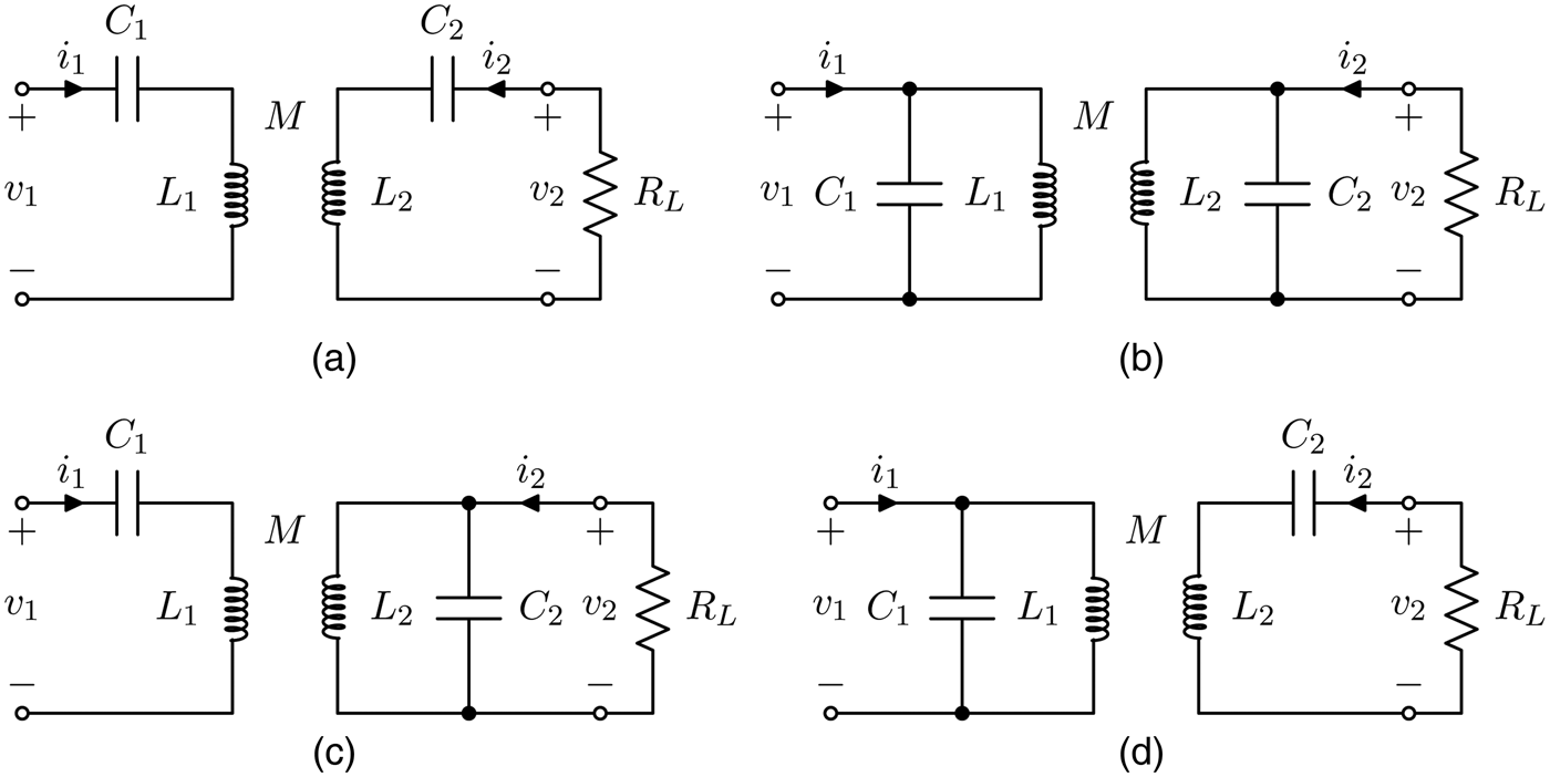
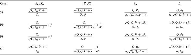
Depending on the arrangement adopted for the resonator on port 1 and the one on port 2, in addition to the PS configuration that has been discussed in the previous part of this paper, three further configurations are possible: the SS, the PP, and the SP configuration (see Fig. 7). The conjugate image impedances corresponding to the four possible configurations and the values of the inductances realizing the optimal design are summarized in Table 1, the normalized impedance matrices, and some discussions are reported in the following.
-
• SS. In this case a series arrangement is considered for both the resonator on port 1 and the resonator on port 2 (i.e. the capacitor C 1 is in series to the inductor L 1, and the capacitor C 2 is in series to the inductor L 2, see Fig. 7(a)). The following impedance matrix can be calculated for the two-port network:
(60) $$Z_{ss} = \left( {\matrix{ {\displaystyle{1 \over {Q_1}}} & {\displaystyle{{j k} \over n}} \cr {\displaystyle{{j k} \over n}} & {\displaystyle{1 \over {Q_2 n^2}}} \cr}} \right)X_0.$$

Accordingly, the expression of the conjugate image impedances is:
 $$Z_{c1,ss} = \displaystyle{{\sqrt {Q_1 Q_2 k^2 + 1}} \over {Q_1}} X_0, $$
 $$Z_{c2,ss} = \displaystyle{{\sqrt {Q_1 Q_2 k^2 + 1}} \over {Q_2 n^2}} X_0.$$
It can be seen that both Z c1,ss and Z c2,ss are purely resistive; as a consequence, no compensating reactances are necessary. More specifically, the inductances realizing the optimal design are:
 $$L_{1,ss} = \displaystyle{{Q_1 R_o} \over {\omega _0 \sqrt {Q_1 Q_2 k^2 + 1}}}, $$
 $$L_{2,ss} = \displaystyle{{Q_2 R_L} \over {\omega _0 \sqrt {Q_1 Q_2 k^2 + 1}}}. $$
-
• PP. In this case a parallel arrangement is considered for both the resonator on port 1 and the resonator on port 2 (i.e. the capacitor C 1 is in parallel with the inductor L 1, and the capacitor C 2 is in parallel with the inductor L 2, see Fig. 7(b)). The following impedance matrix can be calculated for the two-port network:
(65)
$$Z_{pp} = \left( {\matrix{ {\displaystyle{{Q_1} \over {Q_1 Q_2 k^2 + 1}} - j} & { - \displaystyle{{j Q_1 Q_2 k} \over {\left( {Q_1 Q_2 k^2 + 1} \right) n}}} \cr { - \displaystyle{{j Q_1 Q_2 k} \over {\left( {Q_1 Q_2 k^2 + 1} \right) n}}} & {\displaystyle{{Q_2} \over {\left( {Q_1 Q_2 k^2 + 1} \right) n^2}} - \displaystyle{j \over {n^2}}} \cr}} \right) X_0.$$

Accordingly, the expression of the conjugate image impedances is:
 $$Z_{c1,pp} = \left( {\displaystyle{{Q_1} \over {\sqrt {Q_1 Q_2 k^2 + 1}}} + j} \right) X_0, $$
 $$Z_{c2,pp} = \left( {\displaystyle{{Q_2} \over {\sqrt {Q_1 Q_2 k^2 + 1} n^2}} + \displaystyle{j \over {n^2}}} \right) X_0.$$
It can be seen that both Z c1,pp and Z c2,pp have a non-zero imaginary part; as a consequence, it is necessary to add a compensating reactance on both port 1 and port 2. More specifically, the parameters realizing the optimal design are:
 $$X_{c1,pp} = \omega L_1, $$
 $$X_{c2,pp} = \omega L_2, $$
 $$L_{1,pp} = \displaystyle{{\sqrt {Q_1 Q_2 k^2 + 1} R_o} \over {\omega _0 Q_1}},$$
 $$L_{2,pp} = \displaystyle{{\sqrt {Q_1 Q_2 k^2 + 1} R_L} \over {\omega _0 Q_2}}.$$
-
• SP. In this case a series arrangement is considered for the resonator on port 1 (i.e. the capacitor C 1 is in series to the inductor L 1), while a parallel configuration is considered for the resonator on port 2 (i.e. the capacitor C 2 is in parallel with the inductor L 2, see Fig. 7(c)). The impedance matrix of the two-port network is:
(72)
$$Z_{sp} = \left( {\matrix{ {\displaystyle{{Q_1 Q_2 k^2 + 1} \over {Q_1}}} & {\displaystyle{{Q_2 k} \over n}} \cr {\displaystyle{{Q_2 k} \over n}} & {\displaystyle{{Q_2 - j} \over {n^2}}} \cr}} \right) X_0.$$

For the the conjugate image impedances we have:
 $$Z_{c1,sp} = \left( {\displaystyle{{\sqrt {Q_1 Q_2 k^2 + 1}} \over {Q_1}}} \right) X_0,$$
 $$Z_{c2,sp} = \left( {\displaystyle{{Q_2} \over {\sqrt {Q_2 Q_1 k^2 + 1}}} + \displaystyle{j \over {n^2}}} \right) X_0.$$
It can be seen that Z c1,sp is purely resistive while Z c2,sp has a non-zero imaginary part; as a consequence no compesating reactance is necessary on port 1 (i.e., the reactance X c1 is not necessary), while a compensating series reactances X c2 has to be added on port 2. More specifically, the parameters realizing the optimal design are:
 $$X_{c2,sp} = \omega L_2,$$
 $$L_{1,sp} = \displaystyle{{Q_1 R_o} \over {\omega _0 \sqrt {Q_1 Q_2 k^2 + 1}}}, $$
 $$L_{2,sp} = \displaystyle{{\sqrt {Q_1 Q_2 k^2 + 1} R_L} \over {\omega _0 Q_2}}.$$
Considering that the proposed design approach allows maximizing the performance independently of the port where the generator/load is connected to, the PS and SP schemes are completely equivalent; in both cases, by adding to the two-port network the reactance X c1 or X c2 an impedance matrix where all the terms are purely resistive is obtained. According to the theory developed in Section IV, the performance of the link, which corresponds to these schemes are the ones summarized in (54)–(56). As for the impedance matrices of the PP and the SS schemes, they are always complex; in particular, for these schemes the term z 21 is purely imaginary even after the compensation that is necessary for the PP scheme. However, as demonstrated in the Appendix, the performance of the link corresponding to these schemes are still given by (54)–(56).
Possible schemes for coupled resonators. (a) SS configuration, (b) PP configuration, (c) SP configuration, and (d) PS configuration. The case of ideal resonators with zero-losses (i.e. the case where R1 and R2 are equal to zero) is depicted.

Conjugate image impedances at port 1 (Z c1) and port 2 (Z c2). Inductance values for given R o , R L .

Additionally, from Table 1, it can be seen that in the case of a resonator using a series configuration the inductance necessary for realizing the optimal design has a dependence on the coupling coefficient k of the type
 ${1 / {\sqrt {Q_1 Q_2 k^2 + 1}}} $
, while in the case of a resonator using a parallel configuration it has a dependence on k of the type
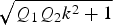 $\sqrt {Q_1 Q_2 k^2 + 1} $
. As a consequence, for equal values of the problem data (i.e., for equal values of R
o
, R
L
, k, Q
1, and Q
2), the optimal values of L
1 and L
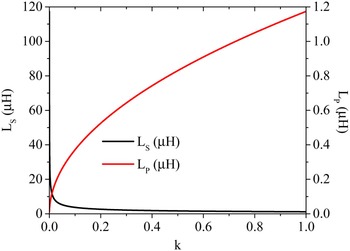
2 are very different for a series or a shunt configuration. This consideration is highlighted in Fig. 8, where the inductances realizing the optimal design are reported for k varying between 0 and 1. The case of a WPT link using resonators with a quality factor equal to 100 (i.e. Q
1 = Q
2 = 100) and with the requirement of having at both an input and a load impedance of 50 Ω (i.e.
 $R_o = R_L = 50 \;\Omega $
) is reported. L
S
is the inductance necessary in the case of a resonator using a series configuration, while L
P
is the inductance necessary in the case of a resonator using a parallel configuration. As it can be seen, in general, for a given value of k, very different values of the inductance are necessary depending on whether the resonator uses a parallel or a series configuration.
Inductances realizing the optimal design for different values of the coupling coefficient k. The following values have been assumed: Q 1 = Q 2 = 100, R o = R L = 50 Ω; while k is varied between 0 and 1. L S is the inductance necessary in the case of a resonator using a series configuration, while L P is the inductance necessary in the case of a resonator using a parallel configuration.

VI. NUMERICAL EXAMPLES
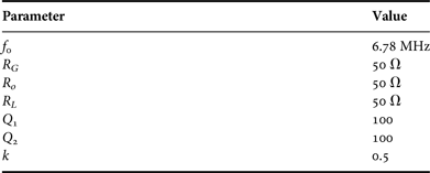
Let us consider the case of a resonant inductive WPT link using a PS configuration and operating at the frequency of 6.78 MHz. The parameters of the link are summarized in Table 2; it is assumed that the coupling coefficient is k = 0.5, that the resonators have a quality factor equal to 100 (i.e. Q
1 = Q
2 = 100). If we select, e.g.
 $R_o = R_L = 50 \;\Omega $
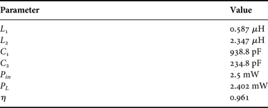
, according to (33) and (34), the value of the parameters realizing the optimal resonant coupling are given in Table 3.
Numerical example analyzed in Section VI.
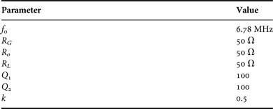
Values of the parameters realizing the optimal design for the example are given in Table 2.
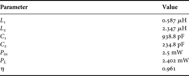
The performance calculated by using the optimal design of the network are also reported.
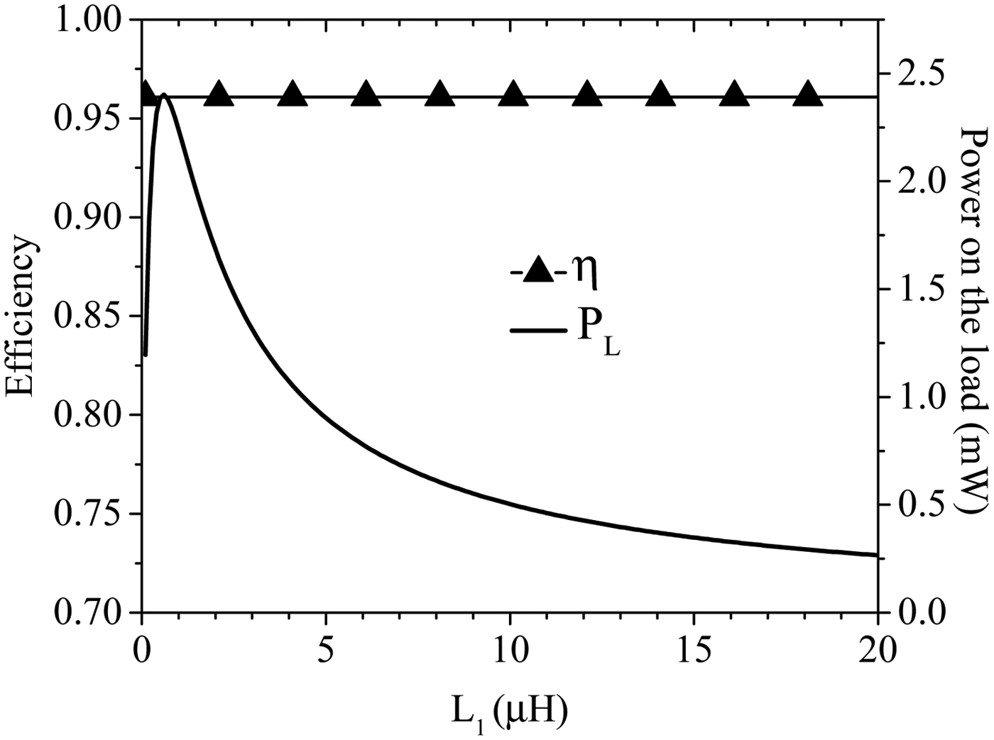
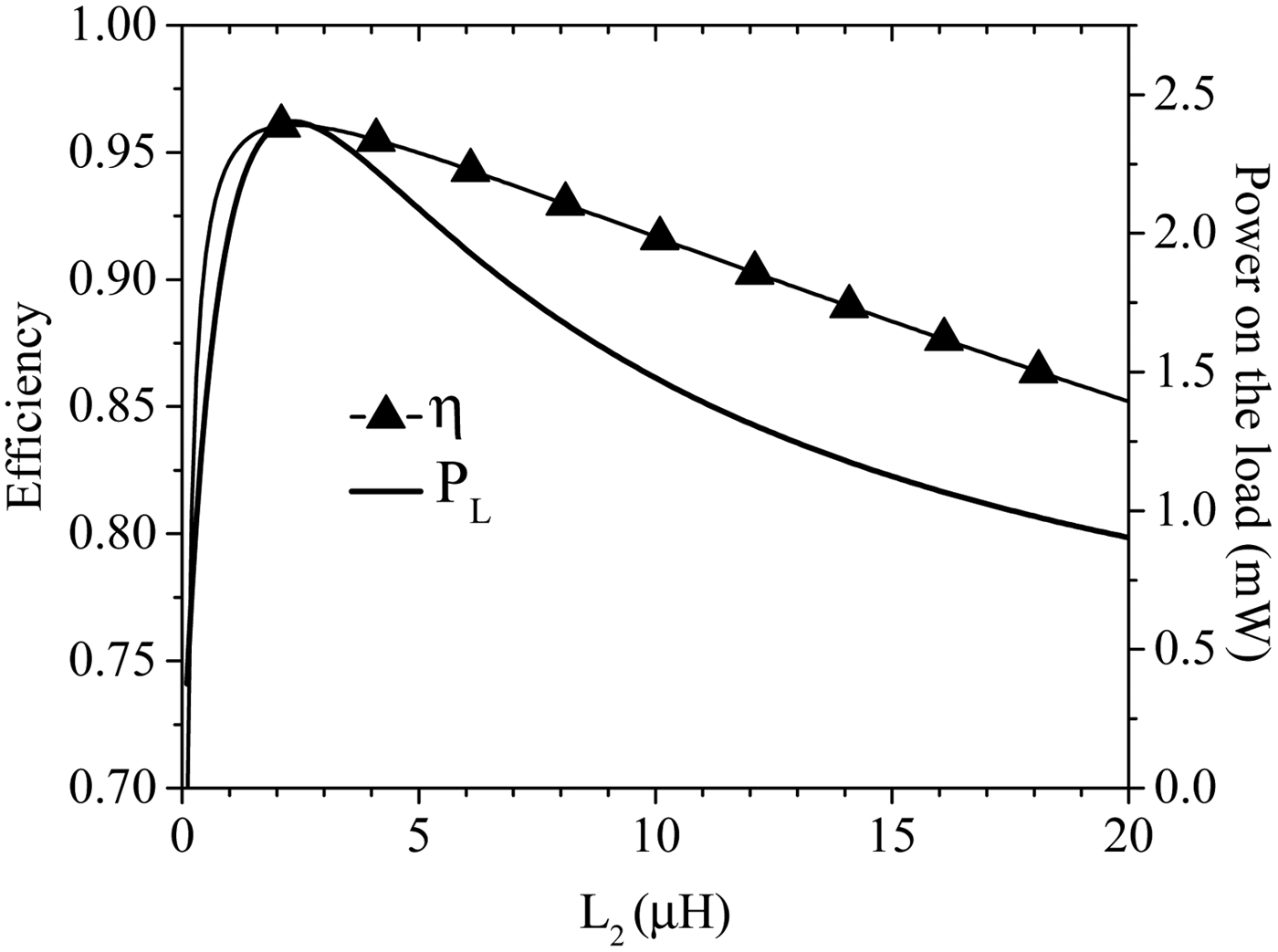
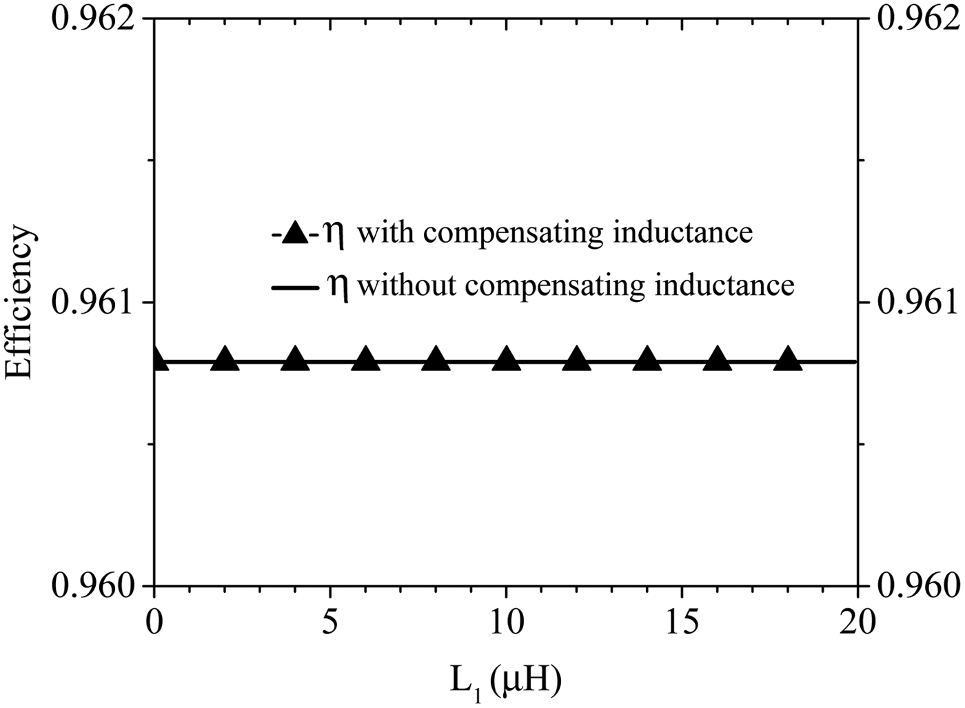
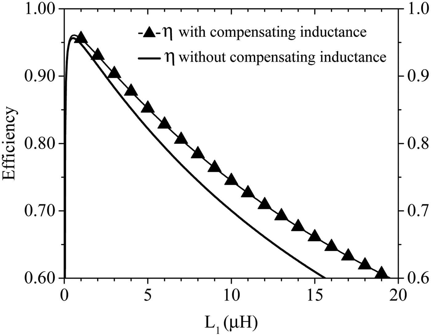
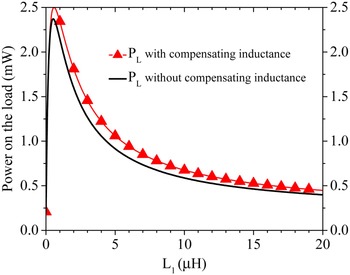
The behavior of the power and of the efficiency as calculated by circuital simulations for the optimal design of the link are given in Figs 9 and 10. In more detail, Fig. 9 illustrates the power on the load and the efficiency calculated by varying the value of the inductance L 1, while the results reported in Fig. 10 have been calculated by varying the value of the inductance L 2. As it can be seen from these figures, the reported results confirm that both the power on the load and the efficiency are maximized when L 1 and L 2 assume the values reported in Table 3. Additionally, according to the analytical expression of the efficiency (53), from Fig. 9 it can be seen that circuital simulations confirm that the efficiency of the link does not depend on L 1. Further results are given in Figs 11 and 12. These figures compare the results calculated for the efficiency and the power on the load with and without the series compensating reactance X c1. As it can be seen, the compensating reactance placed on the input side only affects the output power level, while the efficiency is independent of X c1. On the other hand, if the input and output port roles are exchanged (i.e. the network is operated in SP configuration), and thus the compensating reactance is placed on the output side, its value affects both the output power and the link efficiency, as shown in Figs 13 and 14.
Power on the load and efficiency for the example of Table 2; it is assumed that a 1 V (peak amplitude value) voltage generator is on port 1 and that the load is on port 2. The results obtained by circuit simulations by varying the value of the inductance L
1 are reported; the value of C
1 is also varied according to the formula
 $C_1 = 1/(\omega _0^2 L_1)$
. It can be seen that P
L
is maximized for L
1 = 0.587 μH, while the efficiency η is insensitive from L
1.

Power on the load and efficiency for the example of Table 2; it is assumed that a 1 V (peak amplitude value) voltage generator is on port 1 and that the load is on port 2. The results obtained by circuit simulations by varying the value of the inductance L
2 are reported; the value of C
2 is also varied according to the formula
 $C_2 = 1/(\omega _0^2 L_2)$
. It can be seen that both P
L
and η are maximized for L
2 = 2.347 μH.

Efficiency for the example of Table 2 calculated by circuit simulations by varying the value of the inductance L
1 are reported; the value of C
1 is also varied according to the formula
 $C_1 = 1/(\omega _0^2 L_1)$
. It is assumed that a 1 V (peak amplitude value) voltage generator is on port 1 and that the load is on port 2. The results obtained with and without the series compensating inductance L
1 are reported.

Power on the load for the example of Table 2 calculated by circuit simulations by varying the value of the inductance L
1 are reported; the value of C
1 is also varied according to the formula
 $C_1 = 1/(\omega _0^2 L_1)$
. It is assumed that a 1 V (peak amplitude value) voltage generator is on port 1 and that the load is on port 2. The results obtained with and without the series compensating inductance L
1 are reported.

Efficiency for the example of Table 2 calculated by circuit simulations by varying the value of the inductance L
1 are reported; the value of C
1 is also varied according to the formula
 $C_1 = 1/(\omega _0^2 L_1)$
. It is assumed that a 1 V (peak amplitude value) voltage generator is on port 2 and that the load is on port 1. The results obtained with and without the series compensating inductance L
1 are reported. The maximum value calculated for the case where the compensating inductance L
1 is not present is 0.956, while the one obtained when L
1 is present is 0.961.

Power for the example of Table 2 calculated by circuit simulations by varying the value of the inductance L
1 are reported; the value of C
1 is also varied according to the formula
 $C_1 = 1/(\omega _0^2 L_1)$
. It is assumed that a 1 V (peak amplitude value) voltage generator is on port 2 and that the load is on port 1. The results obtained with and without the series compensating inductance L
1 are reported.

VII. CONCLUSION
The optimal design of a resonant inductive WPT link has been discussed. With regard to the requirement of common practical applications, where the source and the load are usually given, the problem of determining the link parameters maximizing the performance with respect to assigned values of the input and the load impedances has been solved.
Differently from the inverse problem (i.e. the case where the parameters of the link are given and the problem is to find the expression of the optimal terminating impedances), for which previous works demonstrated that different configurations of the link are necessary for maximizing either the power on the load or the efficiency, in this work it has been demonstrated that when the link has to be designed in order to operate with given values of the input and load impedance, there is just one optimal design that allows simultaneously maximizing both the power on the load and the power transfer efficiency of the link. It has been shown that this optimum design can be obtained by imposing that the given input and load resistances coincide with the conjugate image impedances of the two-port network used to realize the link. The general case where the two coupled resonators have a parallel or a series arrangement has been considered and closed-form analytical formulas have been reported for all the possible configurations of the link (SS, SP, PS, and PP). Results obtained by circuital simulations and demonstrating the validity of the reported theory have been also reported and discussed. As a possible development of the present work, it could be of interest to extend the presented solution to a single transmitter–multiple receivers WPT link, which models a practical application where the link is used to power two or more devices.
APPENDIX
Analysis of the performance of the SS and the PP schemes.
In this Appendix, the performance corresponding to an SS and a PP scheme will be analyzed. As already seen in Section V, the SS scheme does not require compensating reactances, while the PP scheme requires a series compensating reactance on both ports. After the addition of the series compensating reactances to the PP scheme, for both the PP and the SS scheme, the impedance matrix is of the type:
 $$Z = \left( {\matrix{ {r_{11}} & {j x_{12}} \cr {j x_{12}} & {r_{22}} \cr}} \right).$$
As it can be seen from (A.1), the term z 12 is complex. Assuming that a voltage generator connected to port 1 and that it has a peak amplitude of 1 V, the following two equations can be obtained for the currents:
 $$1 = I_1\;(R_G + r_{11}) + j I_2 x_{12},$$
 $$0 = I_2\;(R_L + r_{22}) + j I_1 x_{12}$$
with solutions
 $$I_1 = \displaystyle{{R_L + r_{22}} \over {(R_G + r_{11})\;(R_L + r_{22}) + x_{12}^2}},$$
 $$I_2 = - \displaystyle{{ - j x_{12}} \over {(R_G + r_{11})\;(R_L + r_{22}) + x_{12}^2}}.$$
Accordingly, the input resistances
 ${R}^{\prime}_{in} = 1/I_1$
and
 $R_{in} = {R}^{\prime}_{in} - R_G$
are:
 $${R}^{\prime}_{in} = R_G + r_{11} + \displaystyle{{x_{12}^2} \over {R_L + r_{22}}},$$
 $$R_{in} = r_{11} + \displaystyle{{x_{12}^2} \over {R_L + r_{22}}}.$$
The input power
 ${P}^{\prime}_{in} = I_1/2$
and P
in
= R
in
|I
1|2/2 have the following expressions:
 $${P}^{\prime}_{in} = \displaystyle{1 \over 2}\;\displaystyle{{R_L + r_{22}} \over {(R_G + r_{11})\;(R_L + r_{22}) + x_{12}^2}},$$
 $$P_{in} = \displaystyle{1 \over 2}\;\displaystyle{{(R_L + r_{22})\;[r_{11} (R_L + r_{22}) + x_{12}^2 ]} \over {{[(R_G + r_{11})\;(R_L + r_{22}) + x_{12}^2 ]}^2}},$$
while the power on the load P
L
= R
L
|I
2|2/2 and the efficiency η = P
L
/P
in
and
 ${\eta} ^{\prime} = P_L/{P}^{\prime}_{in}$
are written as:
 $$P_L = \displaystyle{1 \over 2}\;\displaystyle{{x_{12}^2 R_L} \over {{[(R_G + r_{11})\;(R_L + r_{22}) + x_{12}^2 ]}^2}},$$
 $$\eta = \displaystyle{{x_{12}^2 R_L} \over {(R_L + r_{22})\;[r_{11} (R_L + r_{22}) + x_{12}^2 ]}},$$
 $${\eta} ^{\prime} = \displaystyle{{x_{12}^2 R_L} \over {(R_L + r_{22})\;[(R_G + r_{11}) (R_L + r_{22}) + x_{12}^2 ]}}.$$
-
• Specialization to the SS case
In the SS case the impedance network parameters take the following form:
 $$r_{11} = \displaystyle{{\omega _0 L_1} \over {Q_1}},$$
 $$x_{12} = \displaystyle{{\omega _0 L_1 k} \over n},$$
 $$r_{22} = \displaystyle{{\omega _0 L_1} \over {Q_2 n^2}}.$$
By inserting the values of (A.13)–(A.15) into (A.7), (A.10), and (A.11), the following expressions are obtained:
 $$R_{in} = \displaystyle{{\omega _0 L_1[Q_2 R_L + \omega _0 L_2(Q_1 Q_2 k^2 + 1)]} \over {Q_1 (\omega _0L_2 + Q_2R_L)}},$$
 $$P_L = \displaystyle{1 \over 2}\;\displaystyle{{\omega _0^2 L_1 Q_1^2 L_2 Q_2^2 k^2 R_L} \over \matrix{[(Q_1R_G + \omega _0L_1)(Q_2R_L + \omega _0L_2) \hfill \cr \quad +\, \omega_0 L_2 Q_1 Q_2 k^2 R_G]^2 \hfill}},$$
 $$\eta = \displaystyle{{\omega _0 Q_1 L_2 Q_2^2 k^2 R_L} \over {(Q_2 R_L + \omega _0 L_2)\;[Q_2 R_L + \omega _0 L_2(Q_1 Q_2 k^2 + 1)]}}.$$
As already discussed for the PS case, it is possible to show that, by selecting L 1 for realizing the desired input impedance (i.e. R in = R o ), and by selecting L 2 for maximizing the efficiency, the results in (63) and (64) are recovered.
When the inductances are the ones given in (63) and (64), for the efficiency and the power on the load corresponding to the optimal design we have:
 $$\eta = \displaystyle{{\zeta - 1} \over {\zeta + 1}},$$
 $${\eta} ^{\prime} = \eta _G \eta,$$
 $$P_L = P_o \eta,$$
which are coincident with (54)–(56).
-
• Specialization to the PP case
In the PP case the impedance network parameters take the following form:
 $$r_{11} = \displaystyle{{\omega _0 L_1 Q_1} \over {Q_1 Q_2 k^2 + 1}},$$
 $$x_{12} = - \displaystyle{{\omega _0 L_1 Q_1 Q_2 k} \over {n(Q_1 Q_2 k^2 + 1)}},$$
 $$r_{22} = \displaystyle{{\omega _0 L_1 Q_2} \over {n^2(Q_1 Q_2 k^2 + 1)}}.$$
By inserting the values of (A.22)–(A.24) into (A.7), (A.10), and (A.11), the following expressions are obtained:
 $$R_{in} = \displaystyle{{\omega _0 L_1 Q_1(R_L + \omega _0 L_2 Q_2)} \over {R_L(Q_1 Q_2 k^2 + 1) + \omega _0 L_2 Q_2}},$$
 $$P_L = \displaystyle{1 \over 2}\;\displaystyle{{\omega _0^2 L_1 Q_1^2 L_2 Q_2^2 k^2 R_L} \over \matrix{[(R_G + \omega _0L_1Q_1)(R_L + \omega _0L_2Q_2) \hfill \cr \quad + \,\omega_0 L_2 Q_1 Q_2 k^2 R_G]^2 \hfill}},$$
 $$\eta = \displaystyle{{\omega _0 Q_1 L_2 Q_2^2 k^2 R_L} \over {(R_L + \omega _0 L_2 Q_2)\;[R_L(Q_1 Q_2 k^2 + 1) + \omega _0 L_2 Q_2]}}.$$
Also in this case it can be easily verified that, by selecting L 1 for realizing R in = R o , and by selecting L 2 for maximizing the efficiency, the results in (70) and (71) are recovered.
When the inductances are the ones given in (70) and (71), the expression given in (A.19) and (A.21) can be recovered for the efficiency of the link and the power on the load, thus demonstrating that the performance of the WPT link are the same for the four analyzed approaches.
 Giuseppina Monti received the Laurea degree in Telecommunication Engineering (with honors) from the University of Bologna, Italy, in 2003, and the Ph.D. in Information Engineering from the University of Salento (Italy), in 2007. She is currently with the Department of Innovation Engineering (University of Salento), where she is a temporary researcher and lecturer in CAD of Microwave circuits and Antennas. Her current research interest includes the analysis and applications of artificial media (such as, for instance, double-negative metamaterials and nano-carbontube), the analysis of electromagnetic compatibility and electromagnetic interference problems in planar microwave circuits, the design and realization of: microwave components and MEMS-based reconfigurable antennas and devices, rectenna systems, systems and devices for wireless power transmission applications. She has co-authored two chapter books and about 100 papers appeared in international conferences and journals.
 Alessandra Costanzo is an Associate Professor of electromagnetic fields at the University of Bologna, Italy. She has authored more than 140 scientific publications on peer reviewed International Journals and conferences, three chapter books, and she holds three international patents. She has developed innovative software platform for the nonlinear/electromagnetic co-simulation of RF systems, excited by modulated sources demonstrating circuit-level analysis of entire MIMO and UWB links, including realistic channel models. She is now involved in wearable energy-autonomous sensors and wireless power transfer systems. She is MC member of the EU COST action WiPE “Wireless power transfer for sustainable electronics” and she chairs WG1: “far-field wireless power transfer”. She is member of the TPC board member of MTT-S IMS, EUMW, WPTC, RFID-TA ICUWB. She is chair of IEEE MTT-S TC-26 “Wireless Energy Transfer and Conversion” and member of IEEE MTT-S TC-24 RFID Technologies. She is IEEE senior member.
 Franco Mastri received the laurea degree (100/100 cum laude) in Electronic Engineering from the University of Bologna, Italy, in 1985. From 1990 to 2004, he was a Research Associate with the Department of Electrical Engineering, University of Bologna, where he has been an Associate Professor of electrotechnics since 2005. His main research interests include nonlinear-circuit simulation and design techniques (with special emphasis on CAD techniques for large-size problems), nonlinear RF device modeling, nonlinear/RF co-simulation of RF systems, stability and noise analysis of nonlinear circuits.
 Mauro Mongiardo received the laurea degree (110/110 cum laude) in Electronic Engineering from the University of Rome “La Sapienza” in 1983. In 1991 he became Associate Professor of Electromagnetic Fields and from 2001 he is full Professor of Electromagnetic Fields at the University of Perugia. He has been elected Fellow of the IEEE for “for contributions to the modal analysis of complex electromagnetic structures” in 2013. His scientific interests have concerned primarily the numerical modeling of electromagnetic wave propagation both in closed and open structures. His research interests have involved CAD and optimization of microwave components and antennas. He has served in the Technical Program Committee of the IEEE International Microwave Symposium from 1992; from 1994 he is member of the Editorial Board of the IEEE TRANSACTIONS ON MICROWAVE THEORY AND TECHNIQUES. During the years 2008–2010 he has been associate editor of the IEEE TRANSACTIONS ON MICROWAVE THEORY AND TECHNIQUES. He is author or co-author of over 200 papers and articles in the fields of microwave components, microwave CAD and antennas. He is the co-author of the books “Open Electromagnetic Waveguides” (IEE, 1997), and “Electromagnetic Field Computation by Network Methods” (Springer, 2009). Recently, he has co-authored a chapter in the book Wireless Power Transfer – Principles and Engineering Explorations (Intech, 2012), and a chapter in the book Wireless Power Transfer (River publishers, 2012).