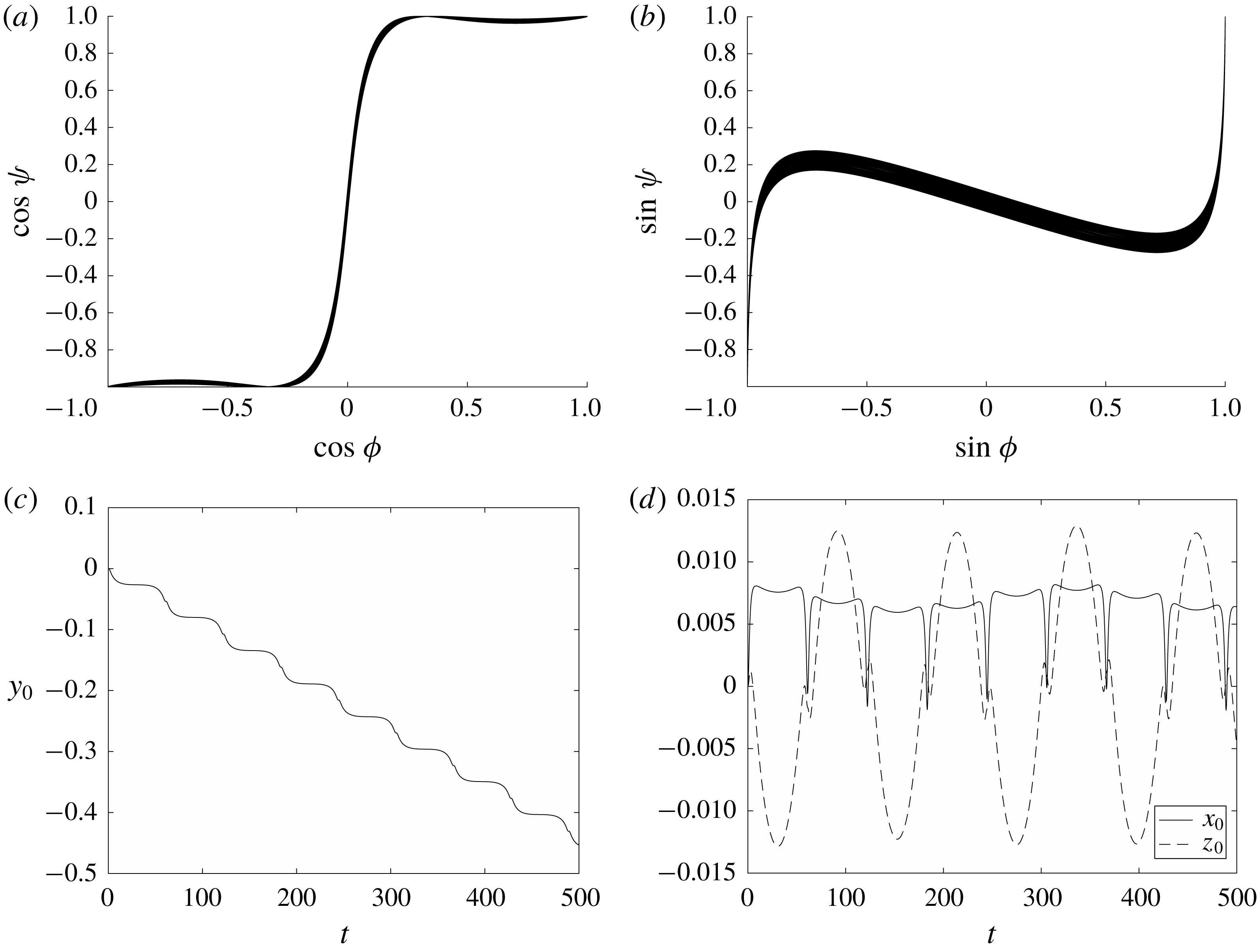
1 Introduction
The motion of particles in fluid flow has been much studied over the years. In a sufficiently dilute suspension, the interactions between particles can be ignored and so we can consider the effect of the fluid flow on a single particle. Furthermore, the motion of small particles is dominated by the local character of the flow, which in many cases is a shear flow; important examples are Poiseuille flow in a cylindrical pipe and Couette flow between parallel plates. For sufficiently small particles in a viscous flow, this local problem can be described by the Stokes equations and the inertia of the particle neglected.
Much of the previous work in this area has focused on ellipsoids. Jeffery (Reference Jeffery1922) first derived analytical expressions for the couple acting on an ellipsoid in a general linear flow and hence derived the equations of rotational motion. A simple analytic solution was found for the case of an axisymmetric ellipsoid (also called a spheroid) in shear flow; the motion is periodic, with the ends of the axis of symmetry tracing out a spherical ellipse. An orbit of this kind is now called a Jeffery orbit.
This work was expanded on by Hinch & Leal (Reference Hinch and Leal1979), who found numerical solutions for the rotational motion of general, non-axisymmetric ellipsoids. They found solutions exhibiting a quasiperiodic structure. Their results were revised by Yarin, Gottlieb & Roisman (Reference Yarin, Gottlieb and Roisman1997), who found, in addition, regions of chaotic behaviour. The chaotic regions are small for particles that are nearly axisymmetric, but grow larger with greater deviations from axisymmetry.
Some attention has also been given to general axisymmetric bodies. Bretherton (Reference Bretherton1962) showed that the rotational motion of an axisymmetric body can be described in terms of a single parameter determined by the shape of the body. Depending on the value of this parameter, the body either behaves like an axisymmetric ellipsoid and follows a Jeffery orbit, or it rotates into one of two opposite, fixed orientations. Bretherton showed that exponentially slender dumbbell-shaped particles can align in shear flow, but rigid particles of such extreme aspect ratios would likely be impossible to construct in practice. More recent work (Borker, Stroock & Koch Reference Borker, Stroock and Koch2018), however, has shown that axisymmetric ring-shaped particles with a non-circular cross-section and of moderate aspect ratio are also able to align in shear flow, and such particles could certainly be constructed.
The other class of bodies considered by Bretherton are those with two (or three) orthogonal planes of symmetry. This class includes both ellipsoids and curved spheroids. The rotational motion of particles with these symmetries can be described in terms of at most three independent parameters. Since the rotational motion is independent of the size of the body, ellipsoids have only two rotational parameters: the two aspect ratios. Hence, bodies in this symmetry class do not in general behave precisely like ellipsoids. However, we will see that the motion is qualitatively very similar.
Finally, some numerical work has been done on the rotation and translation of curved spheroids by Wang et al. (Reference Wang, Tozzi, Graham and Klingenberg2012). They approximated the particles by a series of axisymmetric ellipsoids joined together along the arc of a circle, ignoring hydrodynamic interactions between the different segments. They found that certain initial orientations cause the particles to drift steadily in the direction of the gradient of the shear. Steady drift is to be expected for chiral particles, such as helices, but it was surprising that particles of non-chiral shape can drift in a direction perpendicular to the flow.
In this paper, we aim to elucidate the mathematical underpinnings of the rotational and translational motion of particles with two planes of symmetry. We shall use Kolmogorov–Arnold–Moser (KAM) theory and related ideas to explain the results of Hinch & Leal and Yarin et al. on rotation and of Wang et al. on translation, placing them in the wider context of near-integrable dynamical systems. In particular, we shall be concerned with questions of stability. Are the previously observed quasiperiodic orbits stable? Is the steady drift observed by Wang et al. truly stable or is it merely a transient phenomenon? We shall also give a criterion based on the particle’s shape and initial orientation for whether or not it drifts persistently.
In § 2, we derive the equations of rotational motion for a general body with two planes of symmetry in terms of three parameters that depend on the detailed shape of the body. The generality of our assumptions of symmetry ensures that our results will hold for a wide class of particles, including ellipsoids, curved spheroids, square-based pyramids and particles in the shape of the capital letters A–E, H, I, etc. In § 3, we reduce the continuous-time three-dimensional system to a discrete-time two-dimensional system by using a Poincaré section. We then use KAM theory as applied to reversible maps to explain some qualitative and quantitative features of the motion, as illustrated by numerical simulations for some curved spheroids. Finally, in § 4, we discuss how the symmetries of the orbit of the particle’s orientation determine the possible directions in which the particle can drift persistently.
2 Equations of motion
In this section, we consider bodies with two planes of symmetry and derive the equations governing the motion of a single rigid, non-Brownian, neutrally buoyant particle in an unbounded shear flow with negligible inertia. The motion is thus governed by the Stokes equations with no body force. Though this may seem like a simple, idealised problem, we will find that there is much to understand before some of the assumptions can be relaxed in future work.
2.1 The grand resistance matrix and body symmetries
The Stokes equations are linear in the fluid velocity, so for a general linear flow
 $\boldsymbol{u}^{\infty }=\boldsymbol{U}^{\infty }+\unicode[STIX]{x1D734}^{\infty }\times \boldsymbol{x}+\unicode[STIX]{x1D640}^{\infty }\boldsymbol{\cdot }\boldsymbol{x}$
we have the standard result (e.g. Kim & Karrila Reference Kim and Karrila1991, p. 109) that the force
 $\boldsymbol{F}$
and couple
 $\boldsymbol{G}$
exerted by the particle on the fluid are linearly related to the rates of translation, rotation and extension of the fluid relative to the particle as follows:
 $$\begin{eqnarray}\displaystyle & \displaystyle F_{i}=\unicode[STIX]{x1D608}_{ij}(U_{j}-U_{j}^{\infty })+\unicode[STIX]{x1D609}_{ij}^{\text{T}}(\unicode[STIX]{x1D6FA}_{j}-\unicode[STIX]{x1D6FA}_{j}^{\infty })-\unicode[STIX]{x1D617}_{ijk}E_{jk}^{\infty }, & \displaystyle\end{eqnarray}$$
 $$\begin{eqnarray}\displaystyle & \displaystyle G_{i}=\unicode[STIX]{x1D609}_{ij}(U_{j}-U_{j}^{\infty })+\unicode[STIX]{x1D60B}_{ij}(\unicode[STIX]{x1D6FA}_{j}-\unicode[STIX]{x1D6FA}_{j}^{\infty })-\unicode[STIX]{x1D618}_{ijk}E_{jk}^{\infty }, & \displaystyle\end{eqnarray}$$
 $\unicode[STIX]{x1D608}_{ij},\unicode[STIX]{x1D609}_{ij},\unicode[STIX]{x1D60B}_{ij},\unicode[STIX]{x1D617}_{ijk}$
and
 $\unicode[STIX]{x1D618}_{ijk}$
are tensor coefficients that depend on the shape and orientation of the particle. The tensors
 $\unicode[STIX]{x1D63C}$
,
 $\unicode[STIX]{x1D63D}$
,
 $\unicode[STIX]{x1D63F}$
,
 $\unicode[STIX]{x1D64B}$
and
 $\unicode[STIX]{x1D64C}$
are often written as blocks within the so-called grand resistance matrix (Kim & Karrila Reference Kim and Karrila1991).
We consider two reference frames. The space frame
 $(x,y,z)$
is fixed. In this frame, the particle rotates and the undisturbed shear flow is steady. We take this flow to be
 $\boldsymbol{u}^{\infty }=(y,0,0)$
in appropriate dimensionless units. The body frame
 $(x^{\prime },y^{\prime },z^{\prime })$
rotates with the particle. In this frame, the particle has a fixed orientation and the undisturbed fluid flow changes its orientation but always remains a shear flow.
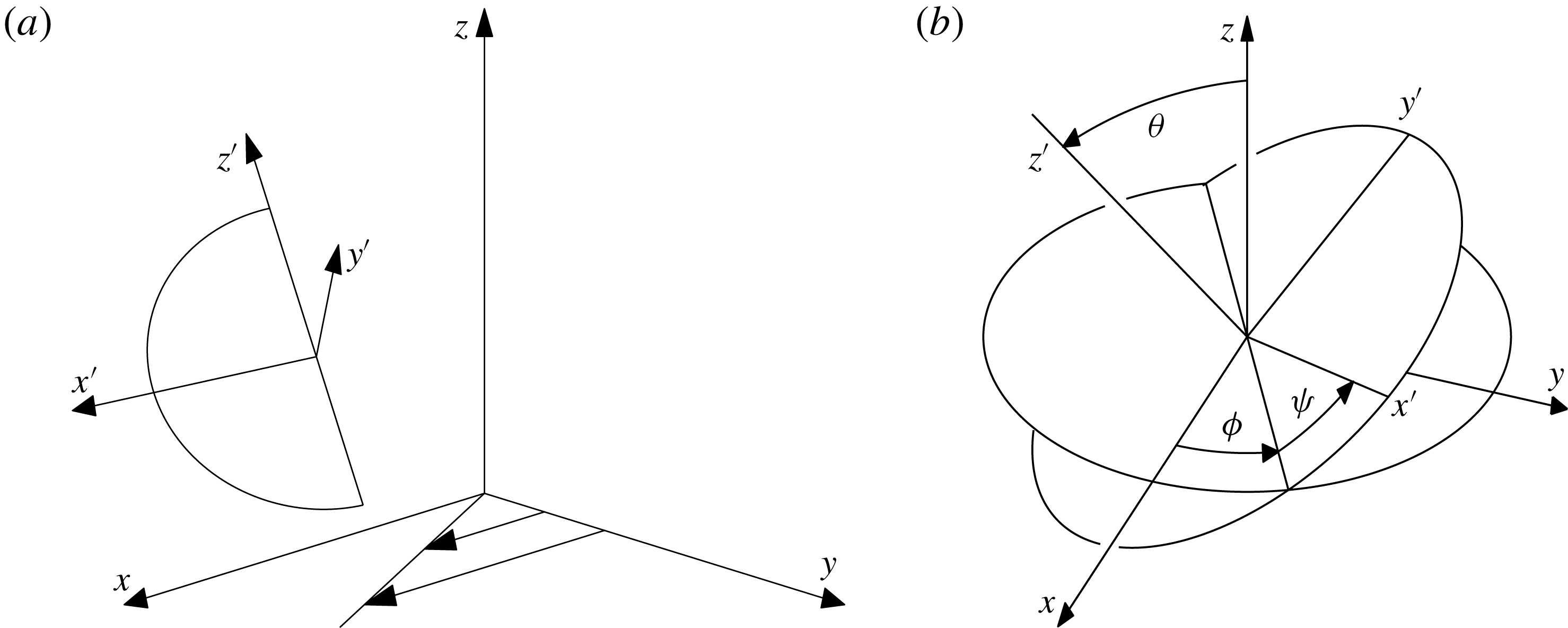
(a) A particle in the shear flow
 $\boldsymbol{u}^{\infty }=(y,0,0)$
. The semicircular particle lies in the body-frame plane
 $y^{\prime }=0$
and has two planes of symmetry
 $y^{\prime }=0$
and
 $z^{\prime }=0$
with respect to body axes embedded in the particle. (b) A diagram of the Euler angles relating the body frame
 $(x^{\prime },y^{\prime },z^{\prime })$
to the laboratory frame
 $(x,y,z)$
.

Consider a particle with two orthogonal planes of symmetry, as shown in figure 1. (If these planes were not orthogonal, then there would be further planes of symmetry by composition of reflections. The particle would then have at least the set of symmetries of a regular polygon or a circle, and its grand resistance matrix would have a more specialised form than considered here.) We take the orthogonal planes of symmetry to be
 $y^{\prime }=0$
and
 $z^{\prime }=0$
. From these two symmetries, we can deduce by standard reflection and reversibility arguments for Stokes flow that many of the above tensor coefficients are zero in the body frame (see appendix A). Omitting the zero terms, we can write (2.1) in the body frame in the form
 $$\begin{eqnarray}\displaystyle \left(\begin{array}{@{}c@{}}F_{1}^{\prime }\\ F_{2}^{\prime }\\ F_{3}^{\prime }\\ G_{1}^{\prime }\\ G_{2}^{\prime }\\ G_{3}^{\prime }\end{array}\right)=\left(\begin{array}{@{}cccccc@{}}\unicode[STIX]{x1D608}_{11} & & & & & \\ & \unicode[STIX]{x1D608}_{22} & & & & \unicode[STIX]{x1D609}_{32}\\ & & \unicode[STIX]{x1D608}_{33} & & \unicode[STIX]{x1D609}_{23} & \\ & & & \unicode[STIX]{x1D60B}_{11} & & \\ & & \unicode[STIX]{x1D609}_{23} & & \unicode[STIX]{x1D60B}_{22} & \\ & \unicode[STIX]{x1D609}_{32} & & & & \unicode[STIX]{x1D60B}_{33}\end{array}\right)\left(\begin{array}{@{}c@{}}U_{1}^{\prime }-U_{1}^{\prime \infty }\\ U_{2}^{\prime }-U_{2}^{\prime \infty }\\ U_{3}^{\prime }-U_{3}^{\prime \infty }\\ \unicode[STIX]{x1D6FA}_{1}^{\prime }-\unicode[STIX]{x1D6FA}_{1}^{\prime \infty }\\ \unicode[STIX]{x1D6FA}_{2}^{\prime }-\unicode[STIX]{x1D6FA}_{2}^{\prime \infty }\\ \unicode[STIX]{x1D6FA}_{3}^{\prime }-\unicode[STIX]{x1D6FA}_{3}^{\prime \infty }\end{array}\right)-\left(\begin{array}{@{}c@{}}\unicode[STIX]{x1D617}_{11}E_{11}^{\prime \infty }+\unicode[STIX]{x1D617}_{33}E_{33}^{\prime \infty }\\ \unicode[STIX]{x1D617}_{12}E_{12}^{\prime \infty }\\ \unicode[STIX]{x1D617}_{13}E_{13}^{\prime \infty }\\ \unicode[STIX]{x1D618}_{23}E_{23}^{\prime \infty }\\ \unicode[STIX]{x1D618}_{13}E_{13}^{\prime \infty }\\ \unicode[STIX]{x1D618}_{12}E_{12}^{\prime \infty }\end{array}\right), & & \displaystyle \nonumber\\ \displaystyle & & \displaystyle\end{eqnarray}$$
where the
 $P$
and
 $Q$
values have been relabelled slightly from (2.1). The symmetries of the particle allow us to decouple the rotations about the axes of the body frame. Rotation about the
 $x^{\prime }$
-axis is associated with row 4 of (2.2); rotation about
 $y^{\prime }$
is associated with rows 3 and 5; rotation about
 $z^{\prime }$
is associated with rows 2 and 6. It is a consequence of the reciprocal theorem for Stokes flow that the matrix in (2.2) is positive–definite and hence invertible, and this decoupling of rotations about different axes reduces the cumbersome inversion of a general
 $6\times 6$
matrix to the inversion of two
 $2\times 2$
matrices. By imposing that the particle is force free and torque free, we can thus deduce simple expressions for the components of the angular velocity
 $\unicode[STIX]{x1D734}^{\prime }$
in terms of the fluid’s far-field rates of rotation and extension,
 $\unicode[STIX]{x1D734}^{\prime \infty }=(1/2)\unicode[STIX]{x1D735}\times \boldsymbol{u}^{\prime \infty }$
and
 $\unicode[STIX]{x1D640}^{\prime \infty }=1/2(\unicode[STIX]{x1D735}\boldsymbol{u}^{\prime \infty }+(\unicode[STIX]{x1D735}\boldsymbol{u}^{\prime \infty })^{\text{T}})$
, respectively.
2.2 Equations for rotation
To relate the velocities in the body frame to those in the space frame, we parameterise the orientation of the particle in terms of the Euler angles. We use the same convention as Hinch & Leal (Reference Hinch and Leal1979). The orientation of the body is defined as follows: the particle begins with the space-frame and body-frame axes aligned. Keeping the space frame fixed, the particle is rotated through an angle
 $\unicode[STIX]{x1D719}\in (-\unicode[STIX]{x03C0},\unicode[STIX]{x03C0}]$
about the
 $z^{\prime }$
-axis, then through
 $\unicode[STIX]{x1D703}\in [0,\unicode[STIX]{x03C0}]$
about the
 $x^{\prime }$
-axis, then through
 $\unicode[STIX]{x1D713}\in (-\unicode[STIX]{x03C0},\unicode[STIX]{x03C0}]$
about the
 $z^{\prime }$
-axis, as shown in figure 1. To convert between the body frame,
 $(x^{\prime },y^{\prime },z^{\prime })$
, and the space frame,
 $(x,y,z)$
, we use the relationship
 $\boldsymbol{x}^{\prime }=\unicode[STIX]{x1D64D}\boldsymbol{\cdot }\boldsymbol{x}$
, where the rotation matrix
 $\unicode[STIX]{x1D64D}$
is given by (Goldstein, Poole & Safko Reference Goldstein, Poole and Safko2001, p. 153)
 $$\begin{eqnarray}\displaystyle \unicode[STIX]{x1D64D}=\left(\begin{array}{@{}ccc@{}}c\unicode[STIX]{x1D719}\,c\unicode[STIX]{x1D713}-c\unicode[STIX]{x1D703}\,s\unicode[STIX]{x1D719}\,s\unicode[STIX]{x1D713} & s\unicode[STIX]{x1D719}\,c\unicode[STIX]{x1D713}+c\unicode[STIX]{x1D703}\,c\unicode[STIX]{x1D719}\,s\unicode[STIX]{x1D713} & s\unicode[STIX]{x1D703}\,s\unicode[STIX]{x1D713}\\ -c\unicode[STIX]{x1D719}\,s\unicode[STIX]{x1D713}-c\unicode[STIX]{x1D703}\,s\unicode[STIX]{x1D719}\,c\unicode[STIX]{x1D713} & -s\unicode[STIX]{x1D719}\,s\unicode[STIX]{x1D713}+c\unicode[STIX]{x1D703}\,c\unicode[STIX]{x1D719}\,c\unicode[STIX]{x1D713} & s\unicode[STIX]{x1D703}\,c\unicode[STIX]{x1D713}\\ s\unicode[STIX]{x1D703}\,s\unicode[STIX]{x1D719} & -s\unicode[STIX]{x1D703}\,c\unicode[STIX]{x1D719} & c\unicode[STIX]{x1D703}\end{array}\right) & & \displaystyle\end{eqnarray}$$
and we have used the notation
 $c\unicode[STIX]{x1D719}=\cos \unicode[STIX]{x1D719},s\unicode[STIX]{x1D719}=\sin \unicode[STIX]{x1D719}$
etc.
We consider the shear flow
 $\boldsymbol{u}^{\infty }=(y,0,0)$
. The
 $x$
,
 $y$
and
 $z$
directions are, respectively, the streamwise, gradient and vorticity directions. The non-zero components of rotation and extension in the space frame are
 $\unicode[STIX]{x1D6FA}_{3}^{\infty }=-1/2$
and
 $E_{12}^{\infty }=E_{21}^{\infty }=1/2$
. The components in the body frame, which vary depending on the body’s orientation, are given by
 $\unicode[STIX]{x1D734}^{\prime \infty }=\unicode[STIX]{x1D64D}\boldsymbol{\cdot }\unicode[STIX]{x1D734}^{\infty }$
and
 $\unicode[STIX]{x1D640}^{\prime \infty }=\unicode[STIX]{x1D64D}\boldsymbol{\cdot }\unicode[STIX]{x1D640}^{\infty }\boldsymbol{\cdot }\unicode[STIX]{x1D64D}^{\text{T}}$
(see appendix B for formulae for
 $\unicode[STIX]{x1D734}^{\prime \infty }$
and
 $\unicode[STIX]{x1D640}^{\prime \infty }$
in terms of the Euler angles), and we deduce from (2.2) with
 $\boldsymbol{F}=\boldsymbol{G}=\mathbf{0}$
that
 $$\begin{eqnarray}\displaystyle (\unicode[STIX]{x1D6FA}_{1}^{\prime },\unicode[STIX]{x1D6FA}_{2}^{\prime },\unicode[STIX]{x1D6FA}_{3}^{\prime })=(\unicode[STIX]{x1D6FA}_{1}^{\prime \infty }-B_{1}E_{23}^{\prime \infty },\unicode[STIX]{x1D6FA}_{2}^{\prime \infty }-B_{2}E_{13}^{\prime \infty },\unicode[STIX]{x1D6FA}_{3}^{\prime \infty }-B_{3}E_{12}^{\prime \infty }), & & \displaystyle\end{eqnarray}$$
where
 $$\begin{eqnarray}\displaystyle B_{1}=-\frac{\unicode[STIX]{x1D618}_{23}}{\unicode[STIX]{x1D60B}_{11}},\quad B_{2}=\frac{\unicode[STIX]{x1D609}_{23}\unicode[STIX]{x1D617}_{13}-\unicode[STIX]{x1D608}_{33}\unicode[STIX]{x1D618}_{13}}{\unicode[STIX]{x1D608}_{33}\unicode[STIX]{x1D60B}_{22}-\unicode[STIX]{x1D609}_{23}^{2}},\quad B_{3}=\frac{\unicode[STIX]{x1D609}_{32}\unicode[STIX]{x1D617}_{12}-\unicode[STIX]{x1D608}_{22}\unicode[STIX]{x1D618}_{12}}{\unicode[STIX]{x1D608}_{22}\unicode[STIX]{x1D60B}_{33}-\unicode[STIX]{x1D609}_{32}^{2}}. & & \displaystyle\end{eqnarray}$$
Equation (2.4) is the same as for ellipsoids (Hinch & Leal Reference Hinch and Leal1979), but the formulae in (2.5) for the coefficients
 $B_{i}$
are more general. For an ellipsoid with axes in the ratio
 $a_{1}:a_{2}:a_{3}$
, Jeffery (Reference Jeffery1922) showed that
 $$\begin{eqnarray}\displaystyle B_{1}^{ellipsoid}=\frac{a_{3}^{2}-a_{2}^{2}}{a_{3}^{2}+a_{2}^{2}},\quad B_{2}^{ellipsoid}=\frac{a_{1}^{2}-a_{3}^{2}}{a_{1}^{2}+a_{3}^{2}},\quad B_{3}^{ellipsoid}=\frac{a_{2}^{2}-a_{1}^{2}}{a_{2}^{2}+a_{1}^{2}}. & & \displaystyle\end{eqnarray}$$
It can be deduced from (2.6) (Bretherton Reference Bretherton1962) that for an ellipsoid
 $$\begin{eqnarray}\displaystyle B_{1}B_{2}B_{3}+B_{1}+B_{2}+B_{3}=0 & & \displaystyle\end{eqnarray}$$
and so the three shape parameters are not independent. For a general body with only two planes of symmetry, however, the three shape parameters are independent, and so bodies in this class do not in general rotate like some ellipsoid.
From (2.4) we obtain, exactly as Hinch & Leal (Reference Hinch and Leal1979) did for ellipsoids, the following autonomous system of ordinary differential equations for the Euler angles (see appendix B for details),
 $$\begin{eqnarray}\displaystyle \dot{\unicode[STIX]{x1D703}} & = & \displaystyle {\textstyle \frac{1}{2}}\unicode[STIX]{x1D6FC}\,s2\unicode[STIX]{x1D703}\,s2\unicode[STIX]{x1D719}+{\textstyle \frac{1}{2}}\unicode[STIX]{x1D6FD}(-s2\unicode[STIX]{x1D703}\,s2\unicode[STIX]{x1D719}\,c2\unicode[STIX]{x1D713}-2s\unicode[STIX]{x1D703}\,c2\unicode[STIX]{x1D719}\,s2\unicode[STIX]{x1D713}),\end{eqnarray}$$
 $$\begin{eqnarray}\displaystyle \dot{\unicode[STIX]{x1D719}} & = & \displaystyle -{\textstyle \frac{1}{2}}+\unicode[STIX]{x1D6FC}\,c2\unicode[STIX]{x1D719}+\unicode[STIX]{x1D6FD}(-c\unicode[STIX]{x1D703}\,s2\unicode[STIX]{x1D719}\,s2\unicode[STIX]{x1D713}+c2\unicode[STIX]{x1D719}\,c2\unicode[STIX]{x1D713}),\end{eqnarray}$$
 $$\begin{eqnarray}\displaystyle \dot{\unicode[STIX]{x1D713}} & = & \displaystyle -\unicode[STIX]{x1D6FC}\,c\unicode[STIX]{x1D703}\,c2\unicode[STIX]{x1D719}+\unicode[STIX]{x1D6FD}(c^{2}\unicode[STIX]{x1D703}\,s2\unicode[STIX]{x1D719}\,s2\unicode[STIX]{x1D713}-c\unicode[STIX]{x1D703}\,c2\unicode[STIX]{x1D719}\,c2\unicode[STIX]{x1D713})\nonumber\\ \displaystyle & & \displaystyle +\,\unicode[STIX]{x1D6FE}(c^{2}\unicode[STIX]{x1D703}\,s2\unicode[STIX]{x1D719}\,s2\unicode[STIX]{x1D713}-2c\unicode[STIX]{x1D703}\,c2\unicode[STIX]{x1D719}\,c2\unicode[STIX]{x1D713}+s2\unicode[STIX]{x1D719}\,s2\unicode[STIX]{x1D713}),\end{eqnarray}$$
 $\unicode[STIX]{x1D6FC}$
,
 $\unicode[STIX]{x1D6FD}$
and
 $\unicode[STIX]{x1D6FE}$
are defined by
 $$\begin{eqnarray}\displaystyle \unicode[STIX]{x1D6FC}={\textstyle \frac{1}{4}}(B_{2}-B_{1}),\quad \unicode[STIX]{x1D6FD}={\textstyle \frac{1}{4}}(B_{2}+B_{1}),\quad \unicode[STIX]{x1D6FE}={\textstyle \frac{1}{4}}B_{3}. & & \displaystyle\end{eqnarray}$$
We observe that these equations describe the motion of any particle with two planes of symmetry, not just ellipsoids, and that we have obtained explicit expressions for the parameters
 $\unicode[STIX]{x1D6FC}$
,
 $\unicode[STIX]{x1D6FD}$
and
 $\unicode[STIX]{x1D6FE}$
in terms of the grand resistance matrix, which can be determined numerically for any shape of particle.
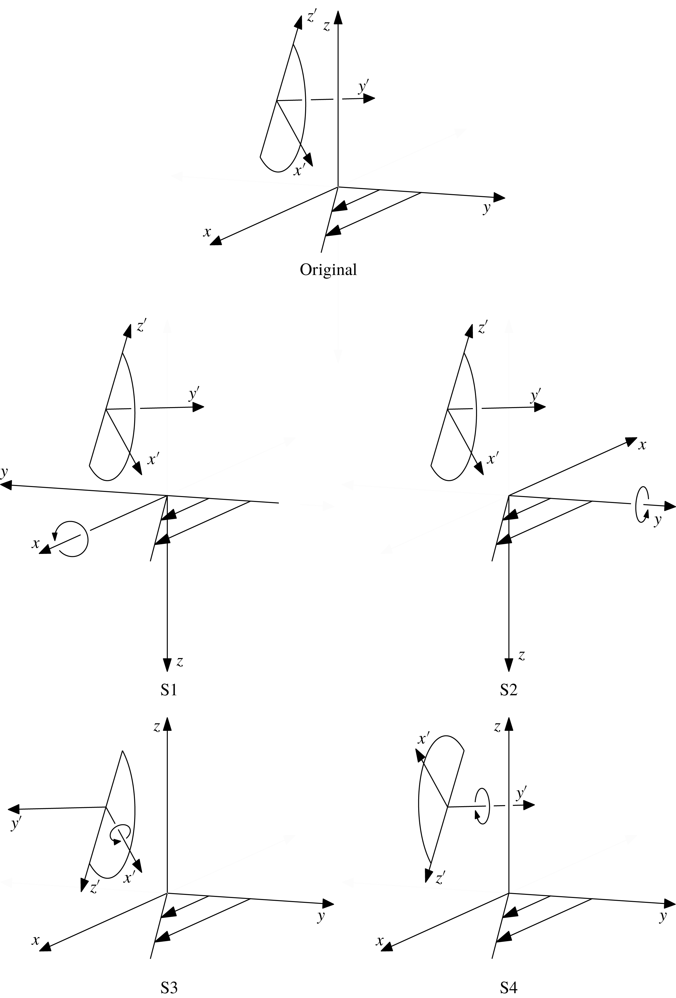
The transformations S1–S4. The axis of rotation is indicated by a small loop. S1 and S2 rotate the space-frame axes and reverse time such that the particle and shear flow are unaffected, resulting in the same motion. S3 rotates the particle by
 $\unicode[STIX]{x03C0}$
about the
 $x^{\prime }$
-axis, but the particle’s two planes of symmetry ensure that it has
 $\unicode[STIX]{x03C0}$
-rotational symmetry about this axis, so the motion is unaffected. S4 rotates the particle by
 $\unicode[STIX]{x03C0}$
about the
 $y^{\prime }$
-axis, and it is not immediately obvious that this should result in equivalent dynamics. This is shown in figure 3.

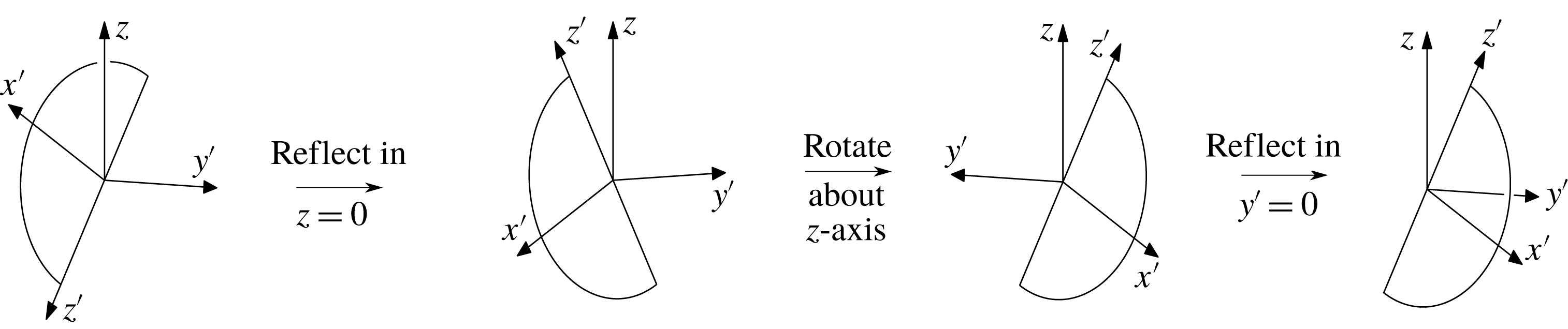
An alternative representation of S4. The viewpoint here is slightly different from that of figure 2, and the
 $x$
-axis points directly out of the page. To get from the S4-transformed particle orientation (left) back to the original orientation (right), one can use the above sequence of transformations. First, reflect the system in
 $z=0$
. This preserves the shear flow. Then rotate the system through an angle
 $\unicode[STIX]{x03C0}$
about
 $z=0$
. This also preserves the shear flow. Finally, reflect the particle in the plane
 $y^{\prime }=0$
. This does not change the particle’s orientation because this is a plane of symmetry. Since each individual transformation preserves the physical system, so too does their composition, S4 (which is its own inverse). Hence, S4 is a symmetry of (2.8).

2.3 Symmetries of the rotational equations
Given the geometrical symmetries of the particle and the shear flow, and the reversibility of Stokes flow, it is not surprising that the differential equations (2.8) possess a great many symmetries. By exploring simple transformations of the variables, we have identified four independent symmetries that generate all the others by composition,
 $$\begin{eqnarray}\displaystyle \begin{array}{@{}l@{}}\text{S1}:\quad (\unicode[STIX]{x1D703},\unicode[STIX]{x1D719},\unicode[STIX]{x1D713},t)\rightarrow (\unicode[STIX]{x03C0}-\unicode[STIX]{x1D703},\unicode[STIX]{x03C0}-\unicode[STIX]{x1D719},\unicode[STIX]{x03C0}+\unicode[STIX]{x1D713},-t),\\ \text{S2}:\quad (\unicode[STIX]{x1D703},\unicode[STIX]{x1D719},\unicode[STIX]{x1D713},t)\rightarrow (\unicode[STIX]{x03C0}-\unicode[STIX]{x1D703},-\unicode[STIX]{x1D719},\unicode[STIX]{x03C0}+\unicode[STIX]{x1D713},-t),\\ \text{S3}:\quad (\unicode[STIX]{x1D703},\unicode[STIX]{x1D719},\unicode[STIX]{x1D713},t)\rightarrow (\unicode[STIX]{x03C0}-\unicode[STIX]{x1D703},\unicode[STIX]{x03C0}+\unicode[STIX]{x1D719},\unicode[STIX]{x03C0}-\unicode[STIX]{x1D713},t),\\ \text{S4}:\quad (\unicode[STIX]{x1D703},\unicode[STIX]{x1D719},\unicode[STIX]{x1D713},t)\rightarrow (\unicode[STIX]{x03C0}-\unicode[STIX]{x1D703},\unicode[STIX]{x03C0}+\unicode[STIX]{x1D719},-\unicode[STIX]{x1D713},t).\end{array} & & \displaystyle\end{eqnarray}$$
As shown in figure 2, physically, S1 corresponds to rotating the shear flow about the
 $x$
-axis and reversing time; S2 corresponds to rotating the shear flow about the
 $y$
-axis and reversing time; S3 corresponds to rotating the particle about its
 $x^{\prime }$
-axis. The rotations in each case are by an angle
 $\unicode[STIX]{x03C0}$
. Clearly, S1, S2 and S3 result in precisely the same physical system as the original, simply with relabelled coordinates. S4 corresponds to rotating the particle by
 $\unicode[STIX]{x03C0}$
about its
 $y^{\prime }$
-axis, which is less obviously the same system. However, the system obtained by implementing the transformation S4 can be returned to the original (see figure 3) by reflecting in the plane
 $z=0$
, then rotating by
 $\unicode[STIX]{x03C0}$
about the
 $z$
-axis and finally reflecting the particle in the plane
 $y^{\prime }=0$
; each of these individual transformations preserves the shear flow, and so S4 is indeed a symmetry of the system.
If we use the physical identification
 $(\unicode[STIX]{x1D703},\unicode[STIX]{x1D719},\unicode[STIX]{x1D713})\equiv (\unicode[STIX]{x1D703},\unicode[STIX]{x1D719}+2m\unicode[STIX]{x03C0},\unicode[STIX]{x1D713}+2n\unicode[STIX]{x03C0})$
for integers
 $m$
and
 $n$
, then each of the transformations S1–S4 is its own inverse and all the transformations commute with each other. The group generated by these elements is thus isomorphic to the abelian group
 $Z=\mathbb{Z}_{2}\times \mathbb{Z}_{2}\times \mathbb{Z}_{2}\times \mathbb{Z}_{2}$
of order 16, where
 $\mathbb{Z}_{2}$
is the cyclic group of order 2. The group structure is given in table 1 for future reference in § 4.
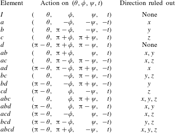
The symmetry group
 $Z$
of the differential equations (2.8). In this table, the elements
 $a$
–
 $d$
have been chosen as generators as they rule out the possibility of translation in particular directions, as discussed in § 4. The transformations S1–S4 (elements
 $ad$
,
 $bd$
,
 $d$
and
 $abcd$
, respectively), however, have some of the simplest physical interpretations.

2.4 Some simple solutions
The equations of motion generally require numerical solution. However, for any particle there exist particularly simple analytic solutions that correspond to the particle rotating with one of its principal axes permanently aligned with the vorticity (
 $z$
-axis): the particle rotates with its
 $x^{\prime }$
-axis aligned with the
 $z$
-axis when
 $\unicode[STIX]{x1D703}=\unicode[STIX]{x03C0}/2=\pm \unicode[STIX]{x1D713}$
, with its
 $y^{\prime }$
-axis aligned when
 $\unicode[STIX]{x1D703}=\unicode[STIX]{x03C0}/2,\unicode[STIX]{x1D713}=0,\pm \unicode[STIX]{x03C0}$
and with its
 $z^{\prime }$
-axis aligned when
 $\unicode[STIX]{x1D703}=0,\unicode[STIX]{x03C0}$
. Rotation about these axes are referred to by Wang et al. (Reference Wang, Tozzi, Graham and Klingenberg2012) as flipping, scooping and spinning, respectively. We shall refer to them collectively as the aligned orbits.
For the case of rotation about the
 $x^{\prime }$
-axis with
 $\unicode[STIX]{x1D703}=\unicode[STIX]{x03C0}/2,~\unicode[STIX]{x1D713}=\pm \unicode[STIX]{x03C0}/2$
, (2.8) reduces to
 $\dot{\unicode[STIX]{x1D719}}=-1/2(1+B_{1}\cos 2\unicode[STIX]{x1D719})$
. The solution (for an appropriate choice of time origin) is
 $$\begin{eqnarray}\displaystyle \tan \unicode[STIX]{x1D719}=\left\{\begin{array}{@{}ll@{}}\displaystyle -\left(\frac{1+B_{1}}{1-B_{1}}\right)^{1/2}\tan \left(\frac{1}{2}\left(\frac{1-B_{1}}{1+B_{1}}\right)^{1/2}t\right)\quad & \text{for }|B_{1}|<1\\ \displaystyle -\left(\frac{B_{1}+1}{B_{1}-1}\right)^{1/2}\tanh \left(\frac{1}{2}\left(\frac{B_{1}-1}{B_{1}+1}\right)^{1/2}t\right)\quad & \text{for }|B_{1}|>1\\ -t\quad & \text{for }B_{1}=1\\ t^{-1}\quad & \text{for }B_{1}=-1\end{array}\right.. & & \displaystyle\end{eqnarray}$$
Hence, this rotation is periodic if
 $|B_{1}|<1$
, and if
 $|B_{1}|\geqslant 1$
then the particle rotates into a fixed orientation and ceases to rotate. Similarly, for rotation about the
 $y^{\prime }$
-axis with
 $\unicode[STIX]{x1D703}=\unicode[STIX]{x03C0}/2,\unicode[STIX]{x1D713}=0$
or
 $\pm \unicode[STIX]{x03C0}$
, (2.8) reduces to
 $\dot{\unicode[STIX]{x1D719}}=-1/2(1-B_{2}\cos 2\unicode[STIX]{x1D719})$
. The solution for
 $\unicode[STIX]{x1D719}$
can then be obtained from (2.11) by replacing
 $B_{1}$
with
 $-B_{2}$
.
Greater care is needed for rotation about the
 $z^{\prime }$
-axis with
 $\unicode[STIX]{x1D703}=0$
or
 $\unicode[STIX]{x03C0}$
. In these cases, the angles
 $\unicode[STIX]{x1D719}$
and
 $\unicode[STIX]{x1D713}$
both describe rotations about the
 $z$
-axis, leading to ambiguity in the Euler-angle representation of the particle’s orientation: the angles
 $\unicode[STIX]{x1D719}$
and
 $\unicode[STIX]{x1D713}$
lose their separate physical identities and the only physical quantity is
 $\unicode[STIX]{x1D719}+\unicode[STIX]{x1D713}$
for
 $\unicode[STIX]{x1D703}=0$
or
 $\unicode[STIX]{x1D719}-\unicode[STIX]{x1D713}$
for
 $\unicode[STIX]{x1D703}=\unicode[STIX]{x03C0}$
.
For rotation about the
 $z^{\prime }$
-axis, (2.8) reduces to
 $$\begin{eqnarray}\displaystyle & \displaystyle \frac{\text{d}}{\text{d}t}(\unicode[STIX]{x1D719}+\unicode[STIX]{x1D713})=-\frac{1}{2}(1+B_{3}\cos 2(\unicode[STIX]{x1D719}+\unicode[STIX]{x1D713}))\quad \text{for }\unicode[STIX]{x1D703}=0, & \displaystyle\end{eqnarray}$$
 $$\begin{eqnarray}\displaystyle & \displaystyle \frac{\text{d}}{\text{d}t}(\unicode[STIX]{x1D719}-\unicode[STIX]{x1D713})=-\frac{1}{2}(1-B_{3}\cos 2(\unicode[STIX]{x1D719}-\unicode[STIX]{x1D713}))\quad \text{for }\unicode[STIX]{x1D703}=\unicode[STIX]{x03C0}. & \displaystyle\end{eqnarray}$$
 $\unicode[STIX]{x1D719}$
with
 $\unicode[STIX]{x1D719}+\unicode[STIX]{x1D713}$
and
 $B_{1}$
with
 $B_{3}$
for
 $\unicode[STIX]{x1D703}=0$
and replacing
 $\unicode[STIX]{x1D719}$
with
 $\unicode[STIX]{x1D719}-\unicode[STIX]{x1D713}$
and
 $B_{1}$
with
 $-B_{3}$
for
 $\unicode[STIX]{x1D703}=\unicode[STIX]{x03C0}$
. (Alternatively, this case could be addressed by returning to (2.4) and permuting the axis labels.)
Hence, if
 $|B_{i}|<1$
for
 $i=1,2,3$
, then the orbits of these simple aligned solutions are periodic. Furthermore, it can be shown from (2.8) that if all
 $|B_{i}|<1$
then
 $\dot{\unicode[STIX]{x1D719}}<0$
in all orientations, and so the particle’s
 $z^{\prime }$
-axis must continually precess around the vorticity direction (
 $z$
-axis) for all time. From (2.6), this condition holds for ellipsoids, and it can be expected to hold for most particle shapes. However, if any
 $|B_{i}|\geqslant 1$
then there exist orientations in which the particle does not rotate at all. Objects in this class include some of the rings with non-circular cross-section studied by Borker et al. (Reference Borker, Stroock and Koch2018), which have
 $B_{2}=-B_{1}>1$
and
 $B_{3}=0$
and which rotate into stable, fixed orientations.
The change in behaviour at
 $|B_{i}|=1$
can be understood physically. A shear flow has equal parts of extension and rotation. The
 $B_{i}$
represent the ratio of the effects of extension and rotation of the fluid on the rotation of the particle. When all of the
 $|B_{i}|<1$
, the fluid’s rotation rate dominates in effect over its strain rate and so the particle rotates unceasingly. However, when
 $|B_{i}|>1$
, there is a component of the fluid’s rate of extension that dominates in effect the corresponding rate of rotation, and so there exist orientations in which the two balance and the particle does not rotate. Thus, the flow (2.8) acquires fixed points when one of the
 $|B_{i}|$
passes through 1.
2.5 Jeffery orbits and integrability
Further analytic solutions can be obtained for a class of particle shapes including, but not limited to, axisymmetric bodies. For example, if we take an axisymmetric ellipsoid with axis lengths in the ratio
 $1:1:r$
, then
 $\unicode[STIX]{x1D6FC}=(1-r^{2})/2(1+r^{2})$
,
 $\unicode[STIX]{x1D6FD}=\unicode[STIX]{x1D6FE}=0$
. The ellipsoid is prolate if
 $r>1$
and oblate if
 $r<1$
. The equations of motion reduce to
 $$\begin{eqnarray}\displaystyle \dot{\unicode[STIX]{x1D703}}={\textstyle \frac{1}{2}}\unicode[STIX]{x1D6FC}\,s2\unicode[STIX]{x1D703}\,s2\unicode[STIX]{x1D719},\quad \dot{\unicode[STIX]{x1D719}}=-{\textstyle \frac{1}{2}}+\unicode[STIX]{x1D6FC}\,c2\unicode[STIX]{x1D719},\quad \dot{\unicode[STIX]{x1D713}}=-\unicode[STIX]{x1D6FC}\,c\unicode[STIX]{x1D703}\,c2\unicode[STIX]{x1D719}. & & \displaystyle\end{eqnarray}$$
The solutions for
 $\unicode[STIX]{x1D719}$
and
 $\unicode[STIX]{x1D703}$
with initial conditions
 $\unicode[STIX]{x1D719}=0$
,
 $\unicode[STIX]{x1D703}=\unicode[STIX]{x1D703}_{0}$
and
 $\unicode[STIX]{x1D713}=\unicode[STIX]{x1D713}_{0}$
can be expressed as
 $$\begin{eqnarray}\displaystyle \tan \unicode[STIX]{x1D719}=-r\tan \frac{rt}{1+r^{2}},\quad \tan \unicode[STIX]{x1D703}=\frac{Cr}{(r^{2}\cos ^{2}\unicode[STIX]{x1D719}+\sin ^{2}\unicode[STIX]{x1D719})^{1/2}}, & & \displaystyle\end{eqnarray}$$
where
 $C=\tan \unicode[STIX]{x1D703}_{0}$
is often called the orbit constant. This solution was first derived by Jeffery (Reference Jeffery1922), and the resulting periodic orbits are termed Jeffery orbits. During a Jeffery orbit, the spheroid’s
 $z^{\prime }$
-axis precesses periodically around the
 $z$
-axis (
 $\unicode[STIX]{x1D719}$
motion). The axis also undergoes periodic nutation (
 $\unicode[STIX]{x1D703}$
motion) in which the inclination of the particle’s axis to the vorticity direction varies between
 $\unicode[STIX]{x1D703}_{0}$
and
 $\arctan (r\tan \unicode[STIX]{x1D703}_{0})$
. The frequency of nutation is exactly twice that of the precession, so the motion of
 $\unicode[STIX]{x1D703}$
and
 $\unicode[STIX]{x1D719}$
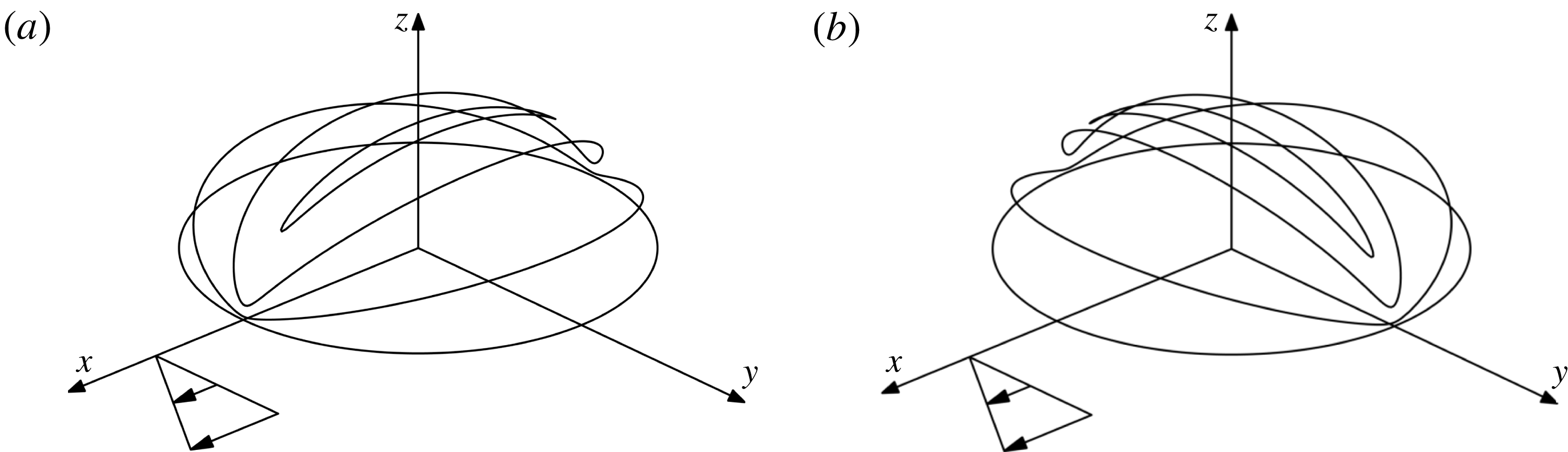
is periodic. A selection of Jeffery orbits is shown in figure 4.
Jeffery orbits: paths traced out by the ends of a spheroid with aspect ratio (a)
 $r=20$
(prolate) and (b)
 $r=1/20$
(oblate). The prolate spheroid rotates most rapidly when its axis is orthogonal to the direction of flow and spends most of its time with its axis aligned near the direction of flow. The situation is reversed for the oblate spheroid, which spends most of its time with its axis aligned nearly perpendicular to the direction of flow.

The particle also spins (
 $\unicode[STIX]{x1D713}$
motion) about its own axis as it precesses. The solution is more complicated, but can still be given analytically in terms of elliptic integrals (see appendix C for details),
 $$\begin{eqnarray}\displaystyle \unicode[STIX]{x1D713}-\unicode[STIX]{x1D713}_{0}=f(C,\unicode[STIX]{x1D719}-n\unicode[STIX]{x03C0})+2nf(C,\unicode[STIX]{x03C0}/2)\quad \text{for }(n-1/2)\unicode[STIX]{x03C0}\leqslant \unicode[STIX]{x1D719}\leqslant (n+1/2)\unicode[STIX]{x03C0}, & & \displaystyle\end{eqnarray}$$
where
 $$\begin{eqnarray}\displaystyle f(C,\unicode[STIX]{x1D719}) & = & \displaystyle \frac{\text{sgn}(C)}{(C^{2}+\unicode[STIX]{x1D716}^{2})^{1/2}}\nonumber\\ \displaystyle & & \displaystyle \times \left\{\left(C^{2}+\frac{1+\unicode[STIX]{x1D716}^{2}}{2}\right)F\left[\arctan \left(\left(\frac{C^{2}+\unicode[STIX]{x1D716}^{2}}{C^{2}+1}\right)^{1/2}\tan \unicode[STIX]{x1D719}\right),\frac{C^{2}(1-\unicode[STIX]{x1D716}^{2})}{C^{2}+\unicode[STIX]{x1D716}^{2}}\right]\right.\nonumber\\ \displaystyle & & \displaystyle -\left.(C^{2}+1)\unicode[STIX]{x1D6F1}\left[\frac{\unicode[STIX]{x1D716}^{2}-1}{C^{2}+\unicode[STIX]{x1D716}^{2}},\arctan \left(\left(\frac{C^{2}+\unicode[STIX]{x1D716}^{2}}{C^{2}+1}\right)^{1/2}\tan \unicode[STIX]{x1D719}\right),\frac{C^{2}(1-\unicode[STIX]{x1D716}^{2})}{C^{2}+\unicode[STIX]{x1D716}^{2}}\right]\right\},\nonumber\\ \displaystyle & & \displaystyle\end{eqnarray}$$
 $$\begin{eqnarray}\displaystyle F(\unicode[STIX]{x1D706},m)=\int _{0}^{\unicode[STIX]{x1D706}}\frac{\text{d}\unicode[STIX]{x1D6FC}}{(1-m\sin ^{2}\unicode[STIX]{x1D6FC})^{1/2}}=\int _{0}^{\text{sin}\,\unicode[STIX]{x1D706}}\frac{\text{d}t}{[(1-t^{2})(1-mt^{2})]^{1/2}} & & \displaystyle\end{eqnarray}$$
and
 $$\begin{eqnarray}\displaystyle \unicode[STIX]{x1D6F1}(n,\unicode[STIX]{x1D706},m)=\int _{0}^{\unicode[STIX]{x1D706}}\frac{1}{1-n\sin ^{2}\unicode[STIX]{x1D6FC}}\frac{\text{d}\unicode[STIX]{x1D6FC}}{(1-m\sin ^{2}\unicode[STIX]{x1D6FC})^{1/2}}=\int _{0}^{\text{sin}\,\unicode[STIX]{x1D706}}\frac{1}{1-nt^{2}}\frac{\text{d}t}{[(1-t^{2})(1-mt^{2})]^{1/2}} & & \displaystyle \nonumber\\ \displaystyle & & \displaystyle\end{eqnarray}$$
are the incomplete elliptic integrals of the first and third kinds, respectively,
 $\unicode[STIX]{x1D716}=1/r$
and
 $\text{sgn}(x)$
denotes the sign of
 $x$
, with
 $\text{sgn}(0)=0$
.
During each period of nutation, in which
 $\unicode[STIX]{x1D719}$
changes from
 $-n\unicode[STIX]{x03C0}$
to
 $-(n+1)\unicode[STIX]{x03C0}$
, the particle rotates about its axis of symmetry by an amount
 $\unicode[STIX]{x0394}\unicode[STIX]{x1D713}(\unicode[STIX]{x1D703}_{0})=2f(\unicode[STIX]{x1D703}_{0},-\unicode[STIX]{x03C0}/2)$
, where
 $\unicode[STIX]{x1D703}_{0}$
is the initial and final value of
 $\unicode[STIX]{x1D703}$
. Since the body is axisymmetric, the fact that it has spun about its axis does not affect the subsequent motion.
From (2.14),
 $C=\tan \unicode[STIX]{x1D703}(r^{2}\cos ^{2}\unicode[STIX]{x1D719}+\sin ^{2}\unicode[STIX]{x1D719})^{1/2}/r$
is a constant of motion, the existence of which means that the system is integrable in the sense that the motion is thus constrained to lie in a two-dimensional surface in phase space. The integrability of (2.13) stems in this case from the condition
 $\unicode[STIX]{x1D6FD}=0$
, which decouples the equation for
 $\dot{\unicode[STIX]{x1D713}}$
from the equations for
 $\dot{\unicode[STIX]{x1D703}}$
and
 $\dot{\unicode[STIX]{x1D719}}$
. This condition is equivalent to
 $B_{1}=-B_{2}$
, which holds for any particle with axisymmetry about the
 $z^{\prime }$
-axis. Axisymmetry also implies that
 $B_{3}=\unicode[STIX]{x1D6FE}=0$
, but this is less important. Thus, if the particle is axisymmetric then the equations of motion are integrable, but the converse is false since it is possible to have
 $B_{1}=-B_{2}$
without
 $B_{3}=0$
.
More generally, the equations are also integrable if
 $B_{2}=-B_{3}$
or
 $B_{3}=-B_{1}$
, as is clear from permuting the axes. Hence, if the particle has
 $B_{i}=-B_{j}$
for any
 $i\neq j$
, then the third axis of the particle traces out one of a family of Jeffery orbits, the family being determined by
 $B_{i}-B_{j}$
. The other
 $B_{k}$
simply determines the rate at which the particle rotates about the third axis. Chaotic motion is not possible for any particles in this class.
2.6 Equations for translation
Before exploring the rotational dynamics further, we derive expressions for the translation of the particle in the body frame. We solve (2.2) with zero force and couple to find that
 $$\begin{eqnarray}\displaystyle & \displaystyle U_{1}^{\prime }=U_{1}^{\prime \infty }-(V_{11}E_{11}^{\prime \infty }+V_{33}E_{33}^{\prime \infty }), & \displaystyle\end{eqnarray}$$
 $$\begin{eqnarray}\displaystyle & \displaystyle U_{2}^{\prime }=U_{2}^{\prime \infty }-V_{12}E_{12}^{\prime \infty }, & \displaystyle\end{eqnarray}$$
 $$\begin{eqnarray}\displaystyle & \displaystyle U_{3}^{\prime }=U_{3}^{\prime \infty }-V_{13}E_{13}^{\prime \infty }, & \displaystyle\end{eqnarray}$$
 $$\begin{eqnarray}\displaystyle V_{11}=-\frac{\unicode[STIX]{x1D617}_{11}}{\unicode[STIX]{x1D608}_{11}},\quad V_{33}=-\frac{\unicode[STIX]{x1D617}_{33}}{\unicode[STIX]{x1D608}_{11}},\quad V_{12}=\frac{\unicode[STIX]{x1D609}_{32}\unicode[STIX]{x1D618}_{12}-\unicode[STIX]{x1D60B}_{33}\unicode[STIX]{x1D617}_{12}}{\unicode[STIX]{x1D608}_{22}\unicode[STIX]{x1D60B}_{33}-\unicode[STIX]{x1D609}_{32}^{2}},\quad V_{13}=\frac{\unicode[STIX]{x1D609}_{23}\unicode[STIX]{x1D618}_{13}-\unicode[STIX]{x1D60B}_{22}\unicode[STIX]{x1D617}_{13}}{\unicode[STIX]{x1D608}_{33}\unicode[STIX]{x1D60B}_{22}-\unicode[STIX]{x1D609}_{23}^{2}}. & & \displaystyle \nonumber\\ \displaystyle & & \displaystyle\end{eqnarray}$$
We find the particle’s velocity in the laboratory frame by using
 $\boldsymbol{U}=\unicode[STIX]{x1D64D}^{T}\boldsymbol{\cdot }\boldsymbol{U}^{\prime }$
, which yields
 $$\begin{eqnarray}\displaystyle U_{1}-y_{0} & = & \displaystyle -(V_{11}E_{11}^{\prime \infty }+V_{33}E_{33}^{\prime \infty })(c\unicode[STIX]{x1D719}\,c\unicode[STIX]{x1D713}-c\unicode[STIX]{x1D703}\,s\unicode[STIX]{x1D719}\,s\unicode[STIX]{x1D713})-V_{12}E_{12}^{\prime \infty }(-c\unicode[STIX]{x1D719}\,s\unicode[STIX]{x1D713}-c\unicode[STIX]{x1D703}\,s\unicode[STIX]{x1D719}\,c\unicode[STIX]{x1D713})\nonumber\\ \displaystyle & & \displaystyle -V_{13}E_{13}^{\prime \infty }s\unicode[STIX]{x1D703}\,s\unicode[STIX]{x1D719},\end{eqnarray}$$
 $$\begin{eqnarray}\displaystyle U_{2} & = & \displaystyle -(V_{11}E_{11}^{\prime \infty }+V_{33}E_{33}^{\prime \infty })(s\unicode[STIX]{x1D719}\,c\unicode[STIX]{x1D713}+c\unicode[STIX]{x1D703}\,c\unicode[STIX]{x1D719}\,s\unicode[STIX]{x1D713})-V_{12}E_{12}^{\prime \infty }(-s\unicode[STIX]{x1D719}\,s\unicode[STIX]{x1D713}+c\unicode[STIX]{x1D703}\,c\unicode[STIX]{x1D719}\,c\unicode[STIX]{x1D713})\nonumber\\ \displaystyle & & \displaystyle +V_{13}E_{13}^{\prime \infty }s\unicode[STIX]{x1D703}\,c\unicode[STIX]{x1D719},\end{eqnarray}$$
 $$\begin{eqnarray}\displaystyle U_{3} & = & \displaystyle -(V_{11}E_{11}^{\prime \infty }+V_{33}E_{33}^{\prime \infty })s\unicode[STIX]{x1D703}\,s\unicode[STIX]{x1D713}-V_{12}E_{12}^{\prime \infty }s\unicode[STIX]{x1D703}\,c\unicode[STIX]{x1D713}-V_{13}E_{13}^{\prime \infty }c\unicode[STIX]{x1D703},\end{eqnarray}$$
 $y_{0}$
is the
 $y$
-coordinate (in the laboratory frame) of the origin
 $\boldsymbol{x}^{\prime }=\mathbf{0}$
of the body frame. As expected, one contribution to the particle’s velocity is simply downstream advection by the surrounding fluid with velocity
 $y_{0}\boldsymbol{e}_{x}$
, independent of the particle’s shape and orientation. We shall not be concerned with this advection; instead, we focus on the additional translations caused by the extensional component of the flow, which depend on the particle’s shape and orientation.
An ellipsoid has reflectional symmetry in three orthogonal planes, as do spheres, cubes and cuboids, which is sufficient to constrain
 $V_{ij}$
to be identically zero for all
 $i,j$
(see appendix A). For these particles, there is no additional translation in any direction. The centre of the particle is simply advected along a streamline. For the general case, where there is reflectional symmetry in only two orthogonal planes, there can be persistent drift across streamlines, as analysed in § 4.
3 Analysis of the equations of rotational motion – KAM theory
3.1 Poincaré sections
In general, the rotational equations (2.8) do not have analytic solutions except for the simple cases discussed previously where one of the particle’s principal axes is permanently aligned with the vorticity. The equations must be solved numerically. From now on, we consider only particles with
 $|B_{i}|<1$
for which
 $\dot{\unicode[STIX]{x1D719}}<0$
in all orientations. This means that we can parameterise the orbits with respect to the angle
 $\unicode[STIX]{x1D719}$
rather than time
 $t$
by using
 $\text{d}/\text{d}t=\dot{\unicode[STIX]{x1D719}}^{-1}\text{d}/\text{d}\unicode[STIX]{x1D719}$
.
Following Hinch & Leal (Reference Hinch and Leal1979) and Yarin et al. (Reference Yarin, Gottlieb and Roisman1997), we reduce the three-dimensional continuous system (2.8) to a two-dimensional discrete system by considering the Poincaré section obtained by plotting
 $\unicode[STIX]{x1D703}$
against
 $\unicode[STIX]{x1D713}$
whenever
 $\unicode[STIX]{x1D719}=-n\unicode[STIX]{x03C0}$
. Physically, this occurs when the particle’s
 $z^{\prime }$
-axis lies in a plane
 $x=\text{const.}$
, orthogonal to the direction of fluid flow. We denote the Poincaré map by
 $$\begin{eqnarray}\displaystyle P:(\unicode[STIX]{x1D703}_{n},\unicode[STIX]{x1D713}_{n})\rightarrow (\unicode[STIX]{x1D703}_{n+1},\unicode[STIX]{x1D713}_{n+1}). & & \displaystyle\end{eqnarray}$$
We can also use the symmetry
 $\unicode[STIX]{x1D713}\rightarrow \unicode[STIX]{x1D713}+\unicode[STIX]{x03C0}$
(denoted
 $abc$
) to parameterise the Poincaré section by
 $(\unicode[STIX]{x1D703},\unicode[STIX]{x1D713})\in [0,\unicode[STIX]{x03C0}]\times (-\unicode[STIX]{x03C0}/2,\unicode[STIX]{x03C0}/2]$
, where we identify mathematically
 $\unicode[STIX]{x1D713}=\unicode[STIX]{x03C0}/2$
with
 $\unicode[STIX]{x1D713}=-\unicode[STIX]{x03C0}/2$
so that the section has a cylindrical topology.
We consider first the case of an axisymmetric particle with
 $B_{1}=-B_{2}$
. The particle’s
 $z^{\prime }$
-axis follows a Jeffery orbit, and so from (2.14) and (2.15) the Poincaré map
 $P(\unicode[STIX]{x1D703}_{n},\unicode[STIX]{x1D713}_{n})$
is simply defined by
 $$\begin{eqnarray}\displaystyle & \displaystyle \unicode[STIX]{x1D703}_{n+1}=\unicode[STIX]{x1D703}_{n}, & \displaystyle\end{eqnarray}$$
 $$\begin{eqnarray}\displaystyle & \displaystyle \unicode[STIX]{x1D713}_{n+1}=\unicode[STIX]{x1D713}_{n}+\unicode[STIX]{x03C0}T(\unicode[STIX]{x1D703}_{n}), & \displaystyle\end{eqnarray}$$
 $\unicode[STIX]{x03C0}T(\unicode[STIX]{x1D703})=2f(\tan \unicode[STIX]{x1D703},-\unicode[STIX]{x03C0}/2)$
and
 $f$
is given by (2.16). In half a Jeffery orbit,
 $\unicode[STIX]{x1D719}$
decreases by
 $\unicode[STIX]{x03C0}$
,
 $\unicode[STIX]{x1D703}$
returns to its original value and
 $\unicode[STIX]{x1D713}$
increases by
 $\unicode[STIX]{x03C0}T(\unicode[STIX]{x1D703})$
. The Poincaré section is therefore very simple. It consists of lines of constant
 $\unicode[STIX]{x1D703}$
.
The function
 $T(\unicode[STIX]{x1D703})$
, sometimes called the rotation number, is the ratio of the frequency of spinning about the particle’s symmetry axis (
 $\unicode[STIX]{x1D713}$
motion) to the frequency of precession of this axis about the vorticity direction (
 $\unicode[STIX]{x1D719}$
motion).
 $T(\unicode[STIX]{x1D703})$
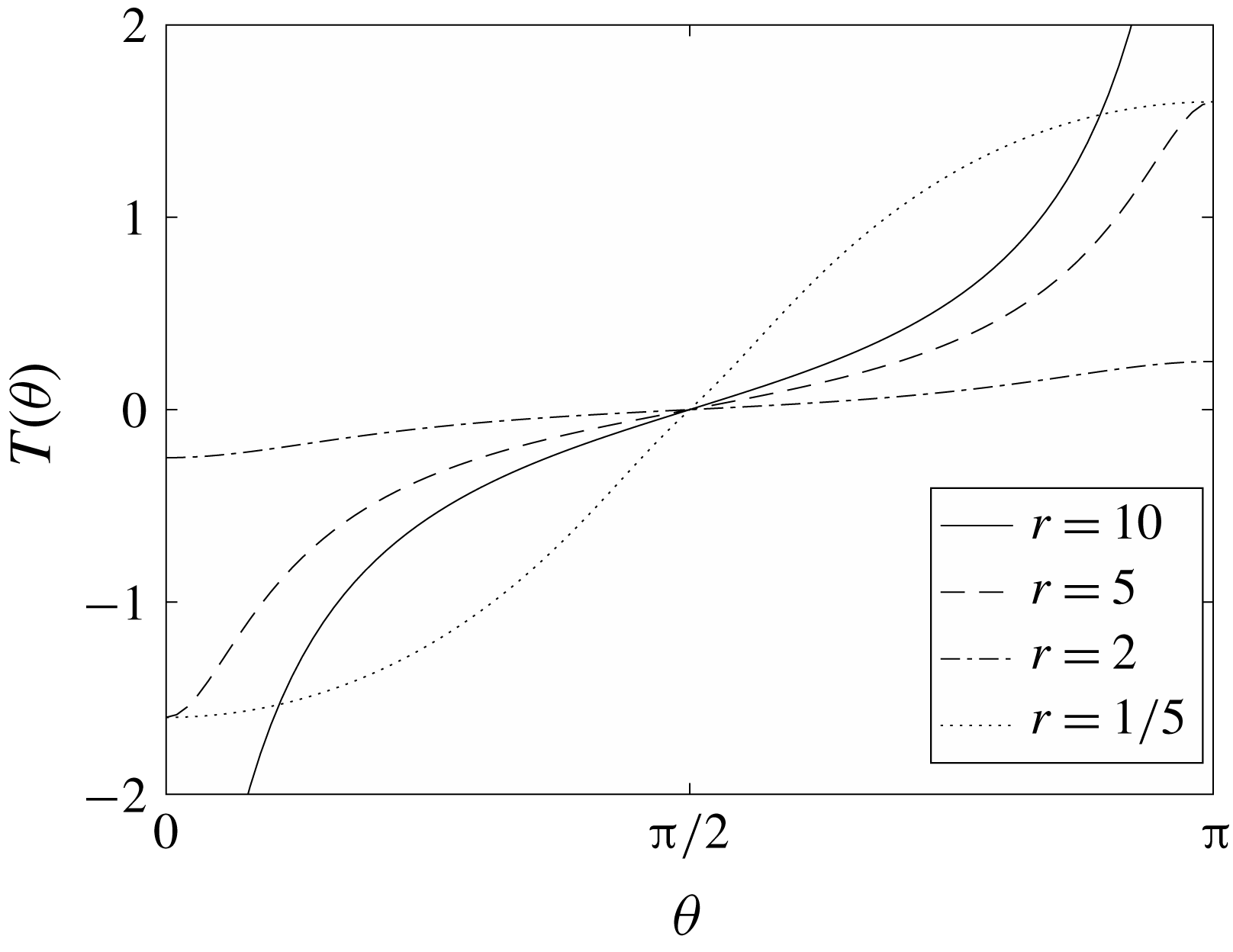
plays a key role in the theory below. Figure 5 shows graphs of
 $T(\unicode[STIX]{x1D703})$
for various axisymmetric ellipsoids with axes in the ratio
 $1:1:r$
. For a sphere,
 $r=1$
and so
 $\unicode[STIX]{x1D6FC}=0$
. Hence, from (2.13),
 $\dot{\unicode[STIX]{x1D713}}=0$
and so a sphere precesses without spinning and
 $T(\unicode[STIX]{x1D703})\equiv 0$
. As the aspect ratio
 $r$
deviates from 1 and the spheroid becomes more prolate or more oblate,
 $T$
increases in size and so the particle spins more during a Jeffery orbit.
 $T(\unicode[STIX]{x1D703})$
is a monotonically increasing function of
 $\unicode[STIX]{x1D703}$
, which means that the Poincaré map (3.2) is an example of a twist map, which can be thought of as twisting points around the cylindrical Poincaré section.
The rotation number
 $T(\unicode[STIX]{x1D703})$
defined by (3.2b
) for an axisymmetric ellipsoid with axes in the ratio
 $1:1:r$
.

For non-axisymmetric particles, which generally have
 $B_{1}\neq -B_{2}$
, the Poincaré map loses the simple form (3.2),
 $\unicode[STIX]{x1D703}$
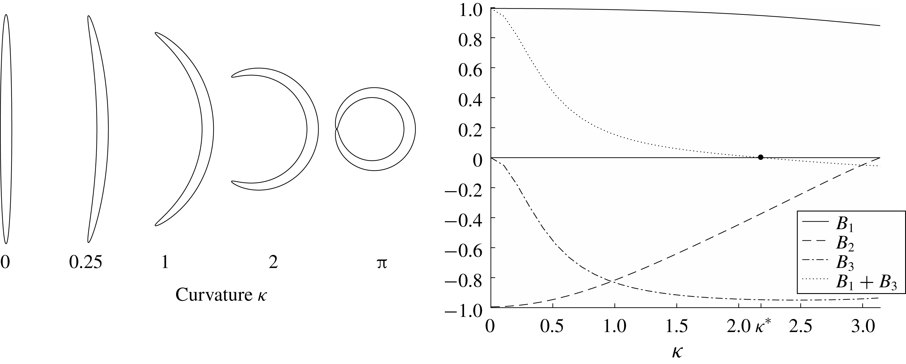
no longer returns to the same value after half a Jeffery orbit, and the Poincaré map is no longer integrable. To illustrate how the Poincaré sections change as we move away from integrability, we consider a family of curved particles, as shown in figure 6(a).
(a) The shapes of a family of curved spheroids of centreline length 2, maximum radius
 $\unicode[STIX]{x1D716}=0.05$
and centreline curvature
 $\unicode[STIX]{x1D705}$
varying between
 $0$
and
 $\unicode[STIX]{x03C0}$
. For
 $\unicode[STIX]{x1D705}=0$
the particle is an axisymmetric ellipsoid. For
 $\unicode[STIX]{x1D705}=\unicode[STIX]{x03C0}$
, the centreline is a complete circle but the particle is not axisymmetric because the cross-sectional area varies along the centreline. (b) The rotational parameters
 $B_{i}$
for the family of curved spheroids. The equations of motion are integrable when
 $\unicode[STIX]{x1D705}=0$
because
 $B_{1}+B_{2}=0$
and when
 $\unicode[STIX]{x1D705}=\unicode[STIX]{x1D705}^{\ast }\approx 2.18$
because
 $B_{1}+B_{3}=0$
.

3.2 Numerical results for curved spheroids
We define these particles to be curved prolate spheroids of length 2 and maximum radius
 $\unicode[STIX]{x1D716}$
, with cross-sectional radius
 $R=\unicode[STIX]{x1D716}(1-s^{2})^{1/2}$
, where
 $s\in [-1,1]$
is the arc length along the centreline. For all numerical simulations, we used
 $\unicode[STIX]{x1D716}=0.05$
, and we used slender-body theory (Johnson Reference Johnson1980) to calculate the coefficients in (2.2). The detailed values do not affect the qualitative behaviour and very similar results are obtained if the coefficients are instead estimated by approximating the particle as a chain of ellipsoids, as in Wang et al. (Reference Wang, Tozzi, Graham and Klingenberg2012).
The centreline is taken to be the arc of a circle with curvature
 $\unicode[STIX]{x1D705}$
, which thus subtends an angle
 $2\unicode[STIX]{x1D705}$
at the centre of the circle. For
 $\unicode[STIX]{x1D705}=0$
, the particle is just a straight prolate spheroid which is axisymmetric about the
 $z^{\prime }$
-axis. Increasing
 $\unicode[STIX]{x1D705}$
increases the particle’s non-axisymmetry.
Figure 6(b) shows the variation of the rotational parameters
 $B_{i}$
with
 $\unicode[STIX]{x1D705}$
. For
 $\unicode[STIX]{x1D705}=0$
the parameters are known analytically from (2.6) to be
 $B_{1}=-B_{2}=(1-\unicode[STIX]{x1D716}^{2})/(1+\unicode[STIX]{x1D716}^{2})\approx 0.995$
and
 $B_{3}=0$
. As
 $\unicode[STIX]{x1D705}$
increases,
 $B_{1}$
decreases slowly and
 $B_{2}$
increases more rapidly, so
 $B_{1}+B_{2}>0$
for
 $\unicode[STIX]{x1D705}>0$
. Hence, the Poincaré map loses the simple form (3.2) and the particle no longer follows Jeffery orbits.
As
 $\unicode[STIX]{x1D705}$
increases,
 $B_{3}$
decreases from
 $0$
and at a value
 $\unicode[STIX]{x1D705}=\unicode[STIX]{x1D705}^{\ast }(\unicode[STIX]{x1D716})\approx 2.18$
, the particle has
 $B_{3}=-B_{1}$
. At this value, the equations of motion are thus integrable again and the curved particle, despite being far from axisymmetric, rotates very much like a particle that is axisymmetric, in that its
 $y^{\prime }$
-axis follows a Jeffery orbit. (The spin of the particle about this axis is not, however, the same as for an axisymmetric particle since
 $B_{2}(\unicode[STIX]{x1D705}^{\ast })\neq 0$
.)
Figures 7–10 show the Poincaré sections for curved spheroids of increasing curvature. To produce these, we calculated a selection of representative orbits of
 $(\unicode[STIX]{x1D703},\unicode[STIX]{x1D719},\unicode[STIX]{x1D713})$
by integrating forwards in time from
 $\unicode[STIX]{x1D719}=0$
to
 $\unicode[STIX]{x1D719}=-N\unicode[STIX]{x03C0}$
starting from a number of different initial conditions (accuracy checks were performed on the numerical integration routine). For each orbit, we then determined the locations of the points
 $(\unicode[STIX]{x1D703}_{n},\unicode[STIX]{x1D713}_{n})$
at which
 $\unicode[STIX]{x1D719}=-n\unicode[STIX]{x03C0}$
,
 $0\leqslant n\leqslant N$
. The Poincaré sections show a dot at each such point. Typically, we took
 $N=400$
, so each orbit is represented by 400 dots.
If an orbit is periodic with
 $(\unicode[STIX]{x1D703}(\unicode[STIX]{x1D719}),\unicode[STIX]{x1D713}(\unicode[STIX]{x1D719}))=(\unicode[STIX]{x1D703}(\unicode[STIX]{x1D719}-q\unicode[STIX]{x03C0}),\unicode[STIX]{x1D713}(\unicode[STIX]{x1D719}-q\unicode[STIX]{x03C0}))$
for some integer
 $q$
, then only
 $q$
distinct points
 $(\unicode[STIX]{x1D703}_{n},\unicode[STIX]{x1D713}_{n})$
are produced in the Poincaré section before the orbit repeats itself. The one-dimensional periodic orbit in
 $(\unicode[STIX]{x1D703},\unicode[STIX]{x1D719},\unicode[STIX]{x1D713})$
phase space thus appears as a
 $q$
-cycle in the Poincaré section. If the orbit is quasiperiodic, consisting of two or more periodic motions with incommensurate frequencies, then the orbit never exactly repeats itself. In
 $(\unicode[STIX]{x1D703},\unicode[STIX]{x1D719},\unicode[STIX]{x1D713})$
phase space, the orbit eventually densely covers a two-dimensional surface topologically equivalent to a torus. This appears as a one-dimensional curve in the Poincaré section. If the orbit is chaotic, then it fills a three-dimensional region in
 $(\unicode[STIX]{x1D703},\unicode[STIX]{x1D719},\unicode[STIX]{x1D713})$
phase space and appears as a sea of dots covering a two-dimensional region in the Poincaré section.
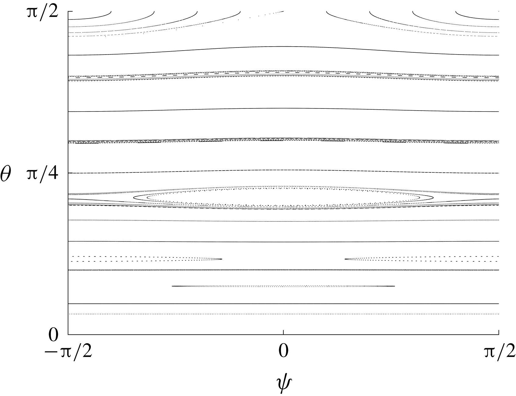
The Poincaré section for a slightly curved spheroid with centreline curvature
 $\unicode[STIX]{x1D705}=0.025$
. Only the lower half of the section is shown, and the upper half is obtained by reflection in
 $\unicode[STIX]{x1D703}=\unicode[STIX]{x03C0}/2$
. Most of the curves representing quasiperiodic orbits wrap around the cylindrical parameter space
 $-\unicode[STIX]{x03C0}/2\leqslant \unicode[STIX]{x1D713}\leqslant \unicode[STIX]{x03C0}/2$
, in the same way as for an axisymmetric particle. There are also islands of closed curves, for example around
 $(0,0.21\unicode[STIX]{x03C0})$
, for which
 $\unicode[STIX]{x1D713}_{n}$
takes only a limited set of values.

(a) Poincaré section for a curved spheroid with
 $\unicode[STIX]{x1D705}=0.075$
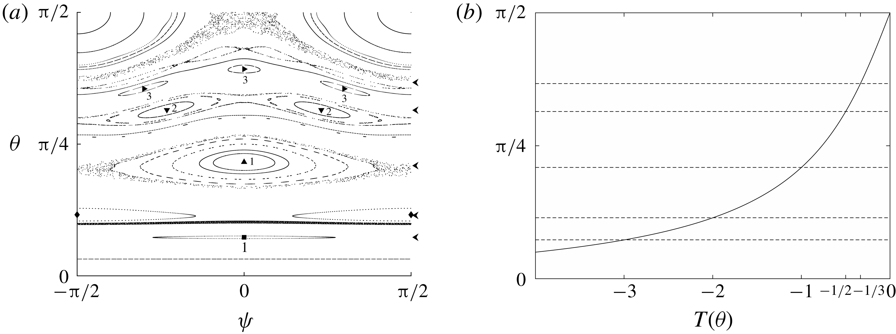
. The islands are larger than in figure 7 and some chains of islands are visible (symbols and numbers denote the length of the chain). Some bands of chaos are visible as fuzzy, dotted regions surrounding the larger islands. (b) The rotation number
 $T(\unicode[STIX]{x1D703})$
for orbits of the axisymmetric ellipsoid with the same value of
 $\unicode[STIX]{x1D6FC}$
. The dotted lines are at the same values of
 $\unicode[STIX]{x1D703}$
as the arrows to the right of (a). This shows the correspondence between the rational values of
 $T(\unicode[STIX]{x1D703})$
and the
 $\unicode[STIX]{x1D703}$
values of the islands in the Poincaré section.

(a) Poincaré section for a curved spheroid with
 $\unicode[STIX]{x1D705}=0.0875$
. Some sub-island chains are visible within and surrounding the larger islands, such as the chain of three islands within the larger island centred on
 $(0,0.21\unicode[STIX]{x03C0})$
. The symbols show periodic orbits that give rise to steady drift (see § 4) and are marked according to the directions in which the particle drifts. (b) The Poincaré section for a curved spheroid with
 $\unicode[STIX]{x1D705}=0.25$
is almost entirely chaotic.

Poincaré sections for curved spheroids with (a)
 $\unicode[STIX]{x1D705}=2.15<\unicode[STIX]{x1D705}^{\ast }$
, (b)
 $\unicode[STIX]{x1D705}=2.2>\unicode[STIX]{x1D705}^{\ast }$
. We show a different range of
 $\unicode[STIX]{x1D703}$
and
 $\unicode[STIX]{x1D713}$
in these sections to better highlight the differences between the behaviours of the particle for
 $\unicode[STIX]{x1D705}<\unicode[STIX]{x1D705}^{\ast }$
and
 $\unicode[STIX]{x1D705}>\unicode[STIX]{x1D705}^{\ast }$
. At
 $\unicode[STIX]{x1D705}=\unicode[STIX]{x1D705}^{\ast }$
, the Poincaré section would show a line of fixed points at
 $\unicode[STIX]{x1D713}=\unicode[STIX]{x03C0}/2$
, corresponding to the particle rotating periodically with its
 $y^{\prime }$
-axis confined to the plane of shear
 $z=\text{const.}$

As noted in § 2.4, all particles have three simple periodic orbits in which one of the body-frame axes is permanently aligned with the
 $z$
-axis, referred to as flipping, scooping and spinning, which can be seen in the Poincaré sections. Flipping, for which the particle’s
 $x^{\prime }$
-axis is aligned, is represented by the fixed point at
 $\unicode[STIX]{x1D713}=\pm \unicode[STIX]{x03C0}/2,\unicode[STIX]{x1D703}=\unicode[STIX]{x03C0}/2$
(these are the same point with the cylindrical topology of the section); scooping, for which the
 $y^{\prime }$
-axis is aligned, is represented by the fixed point at
 $\unicode[STIX]{x1D713}=0,\unicode[STIX]{x1D703}=\unicode[STIX]{x03C0}/2$
; spinning, for which the
 $z^{\prime }$
-axis is aligned, is represented by the line
 $\unicode[STIX]{x1D703}=0$
. This periodic orbit is represented by a line rather than a fixed point due to the aforementioned ambiguity in the Euler-angle representation of the particle’s orientation that occurs when the
 $z$
- and
 $z^{\prime }$
-axes are aligned.
Figure 7 shows the Poincaré section for a nearly straight particle. There are many nearly horizontal curves wrapping around the cylindrical Poincaré section, which represent quasiperiodic orbits. These are very similar to the horizontal lines at constant
 $\unicode[STIX]{x1D703}$
for a simple axisymmetric particle (
 $\unicode[STIX]{x1D705}=0$
) and can be obtained from them by linear perturbation theory. However, there are also some closed curves, termed islands, that do not encircle the cylinder, most prominently enclosing the point
 $(\pm \unicode[STIX]{x03C0}/2,\unicode[STIX]{x03C0}/2)$
and enclosing the point
 $(0,0.21\unicode[STIX]{x03C0})$
.
The curves enclosing the fixed point
 $(\pm \unicode[STIX]{x03C0}/2,\unicode[STIX]{x03C0}/2)$
, which represents flipping, always remain close to it, so the fixed point and the corresponding periodic orbit are stable. The fixed point
 $(0,\unicode[STIX]{x03C0}/2)$
, which represents scooping, is a saddle and therefore unstable. The line
 $\unicode[STIX]{x1D703}=0$
, which represents spinning, is adjacent to nearly horizontal curves, so this orbit is also stable. For a conventional linear stability analysis of these periodic orbits for nearly axisymmetric ellipsoids, see Yarin et al. (Reference Yarin, Gottlieb and Roisman1997).
More features are apparent in figures 8 and 9, which show the Poincaré sections for particles of successively greater curvature. In figures 8(a) and 9(a), the islands of closed curves have grown and we start to see chains of islands and sub-island chains within the larger islands. We also see dotted regions that indicate the presence of chaotic orbits. As we increase the curvature further these chaotic regions grow in size and by
 $\unicode[STIX]{x1D705}=0.25$
(figure 9(b), cf. figure 6) most of the Poincaré section is covered by chaotic orbits. Wang et al. (Reference Wang, Tozzi, Graham and Klingenberg2012) argued, based on a very sparsely filled Poincaré section for comparable
 $\unicode[STIX]{x1D705}$
and
 $\unicode[STIX]{x1D716}$
, that chaotic motion was not possible for these particles, but figure 9(b) quite clearly shows a large number of chaotic orbits.
However, as we increase the curvature further, the sea of chaotic orbits eventually starts to recede as we approach
 $\unicode[STIX]{x1D705}=\unicode[STIX]{x1D705}^{\ast }$
, where
 $B_{1}=-B_{3}$
and the system (2.8) is integrable again. Figure 10 shows Poincaré sections for particles with curvatures just less than and just more than
 $\unicode[STIX]{x1D705}=\unicode[STIX]{x1D705}^{\ast }$
. The Poincaré sections consist almost entirely of closed curves. As the curvature crosses
 $\unicode[STIX]{x1D705}=\unicode[STIX]{x1D705}^{\ast }$
and
 $B_{1}+B_{3}$
crosses 0, the periodic rotations with the
 $x^{\prime }$
-axis aligned and the
 $z^{\prime }$
-axis aligned exchange stability. Although these Poincaré sections look very different to that in figure 7, they are all for nearly integrable Poincaré maps, and the difference here is simply that it is the
 $y^{\prime }$
-axis that undergoes approximate Jeffery orbits rather than the
 $z^{\prime }$
-axis in figure 7.
3.3 The standard map
For small deviations from axisymmetry, the Poincaré map (3.1) is a perturbation to the simple twist map (3.2). The most well-known perturbed twist map is the standard map (Chirikov–Taylor map), defined by
 $$\begin{eqnarray}\displaystyle & \displaystyle \unicode[STIX]{x1D703}_{n+1}=\unicode[STIX]{x1D703}_{n}+K\sin \unicode[STIX]{x1D713}_{n}, & \displaystyle\end{eqnarray}$$
 $$\begin{eqnarray}\displaystyle & \displaystyle \unicode[STIX]{x1D713}_{n+1}=\unicode[STIX]{x1D713}_{n}+\unicode[STIX]{x1D703}_{n}+K\sin \unicode[STIX]{x1D713}_{n}, & \displaystyle\end{eqnarray}$$
 $\unicode[STIX]{x1D713}_{n}$
is taken mod
 $2\unicode[STIX]{x03C0}$
and
 $K$
is a parameter. When
 $K=0$
, the standard map is the simplest possible twist map, with a linear twist. This can be transformed smoothly into the twist map (3.2) for an axisymmetric particle by suitable stretching of
 $\unicode[STIX]{x1D703}$
and
 $\unicode[STIX]{x1D713}$
, so the dynamics is essentially the same. The results of iterating the standard map with
 $K>0$
are shown in figure 11. The variation of the standard map with
 $K$
is remarkably similar to that of the Poincaré map (3.1) with
 $\unicode[STIX]{x1D705}$
: both maps start off with Poincaré sections composed entirely of straight lines, which then give way to nearly straight curves, island chains of closed curves and chaos.
Orbits of the standard map (3.3) for (a)
 $K=0.6$
, (b)
 $K=1$
and (c)
 $K=4$
. For small
 $K$
, most of the section is occupied by closed curves, representing quasiperiodic orbits. As
 $K$
increases and the map becomes further from a twist map, chaotic orbits occupy more and more of the section. Compare these plots with figures 7–9.

The striking similarities between the equations defining the Poincaré map (3.1) and the standard map (3.3), and between the resulting diagrams, suggest that their behaviour can be understood in terms of a common theory. The standard map is an area-preserving perturbation to a twist map and its properties are well understood (Greene Reference Greene1979; Mackay & Percival Reference Mackay and Percival1985) in terms of a broad body of theory comprising the KAM (Kolmogorov–Arnold–Moser) theorem and a number of related ideas due to Poincaré and others, which, for brevity, we shall refer to collectively as KAM theory.
KAM theory describes the behaviour of near-integrable systems for certain classes of perturbations. The best-known applications are to Hamiltonian systems of differential equations and to area-preserving maps such as the standard map. It is less well known that, as discussed in the review by Roberts & Quispel (Reference Roberts and Quispel1992), KAM theory can also be applied to time-reversible differential equations and maps.
As shown in table 1, the differential system (2.8) has eight time-reversing symmetries, which carry over to the Poincaré map
 $P$
. In particular, the symmetry
 $a$
shows that (3.1) is invariant under the time-reversing symmetry
 $G:\unicode[STIX]{x1D713}\rightarrow -\unicode[STIX]{x1D713},n\rightarrow -n$
, which can be restated as
 $GP=P^{-1}G$
. Also,
 $G=G^{-1}$
. Hence the Poincaré map is reversible, and the KAM theorem and related ideas can be applied to explain the behaviour of the rotating particle.
3.4 Interpretation of Poincaré sections in terms of KAM theory
We state here the main results of KAM theory (see Roberts & Quispel Reference Roberts and Quispel1992), as applied to the Poincaré map (3.1). Consider small perturbations to a general twist map, given by
 $$\begin{eqnarray}\displaystyle & \displaystyle \unicode[STIX]{x1D703}_{n+1}=\unicode[STIX]{x1D703}_{n}+\unicode[STIX]{x1D6FF}A_{\unicode[STIX]{x1D703}}(\unicode[STIX]{x1D703}_{n},\unicode[STIX]{x1D713}_{n}), & \displaystyle\end{eqnarray}$$
 $$\begin{eqnarray}\displaystyle & \displaystyle \unicode[STIX]{x1D713}_{n+1}=\unicode[STIX]{x1D713}_{n}+\unicode[STIX]{x03C0}T(\unicode[STIX]{x1D703}_{n})+\unicode[STIX]{x1D6FF}A_{\unicode[STIX]{x1D713}}(\unicode[STIX]{x1D703}_{n},\unicode[STIX]{x1D713}_{n}), & \displaystyle\end{eqnarray}$$
 $\unicode[STIX]{x1D6FF}$
is a small parameter,
 $T$
is a monotonic function of
 $\unicode[STIX]{x1D703}$
and the functions
 $A_{\unicode[STIX]{x1D703}}$
,
 $A_{\unicode[STIX]{x1D713}}$
are
 $\unicode[STIX]{x03C0}$
-periodic in
 $\unicode[STIX]{x1D713}_{n}$
, which is taken to lie in
 $(-\unicode[STIX]{x03C0}/2,\unicode[STIX]{x03C0}/2]$
. For
 $\unicode[STIX]{x1D6FF}A_{\unicode[STIX]{x1D703}}=\unicode[STIX]{x1D6FF}A_{\unicode[STIX]{x1D713}}=K\sin 2\unicode[STIX]{x1D713}_{n}$
and
 $\unicode[STIX]{x03C0}T(\unicode[STIX]{x1D703}_{n})=\unicode[STIX]{x1D703}_{n}$
, we recover the standard map (3.3) after a change of variables, and for
 $\unicode[STIX]{x1D6FF}=0$
and
 $\unicode[STIX]{x03C0}T(\unicode[STIX]{x1D703}_{n})=2f(\unicode[STIX]{x1D703}_{n},-\unicode[STIX]{x03C0}/2)$
, we recover the Poincaré map (3.2). Appropriate choices of the small perturbations
 $A_{\unicode[STIX]{x1D703}}$
and
 $A_{\unicode[STIX]{x1D713}}$
give the Poincaré maps corresponding to nearly axisymmetric particles. For the curved spheroids,
 $\unicode[STIX]{x1D6FF}=B_{1}+B_{2}=O(\unicode[STIX]{x1D705}^{2})$
as
 $\unicode[STIX]{x1D705}\rightarrow 0$
.
Consider the unperturbed map (3.4) with
 $\unicode[STIX]{x1D6FF}=0$
, corresponding to an axisymmetric particle. If
 $T(\unicode[STIX]{x1D703}_{n})$
is a rational number
 $p/q$
, then the motion is periodic and the line
 $\unicode[STIX]{x1D703}=\unicode[STIX]{x1D703}_{n}$
in the Poincaré section is composed of infinitely many
 $q$
-cycles. This happens when the frequencies of precession and spinning are rationally related. If
 $T(\unicode[STIX]{x1D703})$
is irrational, then the motion is quasiperiodic and the line
 $\unicode[STIX]{x1D703}=\unicode[STIX]{x1D703}_{n}$
is composed of quasiperiodic orbits of the Poincaré map, each of which densely covers the line. This happens when the frequencies of precession and spinning are incommensurate, which is the case for almost all values of
 $\unicode[STIX]{x1D703}_{n}$
.
For a general perturbation with no particular properties, almost all of the periodic and quasiperiodic orbits would be destroyed. However, for a reversible perturbation, which is the case applicable to particles in shear, KAM theory guarantees that for small
 $\unicode[STIX]{x1D6FF}$
almost all of the quasiperiodic orbits are instead preserved and merely undergo a small, smooth perturbation, typically of size
 $O(\unicode[STIX]{x1D6FF})$
. These are the slightly curved wrapping orbits seen in figure 7.
However, the periodic orbits are less robust. An even number, usually two for (3.2), of the
 $q$
-cycles with
 $T(\unicode[STIX]{x1D703}_{n})=p/q$
survive as a consequence of the Poincaré–Birkhoff theorem, which is typically stated for area-preserving maps (Moser Reference Moser1968, p. 39), but which also holds for reversible maps (see appendix D). These surviving periodic orbits are known as Poincaré–Birkhoff cycles. Half are of elliptical stability and are surrounded by islands of closed curves. The fact that these curves are closed means that these cycles are neutrally stable, neither attracting nor repelling nearby orbits. The other Poincaré–Birkhoff cycles are of saddle stability and generically give rise to a chaotic band surrounding both the saddle points and the islands around the elliptically stable points. The onset of chaos around one of the periodic aligned orbits was studied numerically and asymptotically in some detail by Yarin et al. (Reference Yarin, Gottlieb and Roisman1997) for a very long, nearly axisymmetric ellipsoid; they presented numerical evidence that chaos occurs due to aperiodic slip-tunnelling between Jeffery orbits near the saddle point. We can now say from the body of KAM theory that this behaviour is generic and occurs not just for ellipsoids but for any particle with two planes of symmetry, and not just for the aligned orbits but near all saddle points of the map.
Figure 8 illustrates the link between the rational values of
 $T(\unicode[STIX]{x1D703}_{n})$
and the locations of the islands. Figure 8(b) shows the function
 $T(\unicode[STIX]{x1D703})$
for an axisymmetric ellipsoid with
 $\unicode[STIX]{x1D716}\approx 0.0529$
, which gives the same value of
 $\unicode[STIX]{x1D6FC}=1/4(B_{2}-B_{1})$
as the curved spheroid with
 $\unicode[STIX]{x1D716}=0.05$
and
 $\unicode[STIX]{x1D705}=0.075$
, whose Poincaré section is shown in figure 8(a). There is a clear correspondence between the
 $\unicode[STIX]{x1D703}$
values of the
 $q$
-cycles at the centres of the major island chains and points at which
 $T(\unicode[STIX]{x1D703})=p/q$
for small
 $q$
.
Furthermore, the islands are of width
 $O(\unicode[STIX]{x1D6FF}^{q/2})$
(see appendix D) and so become smaller as
 $\unicode[STIX]{x1D6FF}$
decreases or as
 $q$
increases. This explains why for small
 $\unicode[STIX]{x1D6FF}$
we only see the islands surrounding the fixed points with
 $q=1$
in figure 7, whereas for larger
 $\unicode[STIX]{x1D6FF}$
we can see islands with
 $q\leqslant 3$
in figure 8(a). Islands with larger
 $q$
are present in both cases but are very thin and hard to find numerically.
In figure 9(a), we see that the larger islands are surrounded by chains of smaller sub-islands, some of which are marked with geometric symbols. This can be understood in terms of the local extension to the global KAM theorem (Roberts & Quispel Reference Roberts and Quispel1992): close to a general elliptic periodic point, any reversible map is locally close to a twist map in the sense that the map can locally be put into the form of (3.4) by a suitable change of coordinates, where
 $\unicode[STIX]{x1D703}$
is now a radial coordinate and
 $\unicode[STIX]{x1D713}$
an angular coordinate local to the elliptic fixed point.
It follows from this extension that we find the same structures around each elliptic periodic point as in the global picture. For example, the islands of closed curves around the elliptic periodic points are the local equivalent of the global invariant curves that wrap around the cylindrical Poincaré section, and both are commonly referred to as KAM curves. Similarly, the sub-island chains around the larger islands are the local equivalent of the larger islands themselves, and the saddles between the sub-islands also lie in thin bands of chaos.
This process of zooming in near an island and finding sub-islands can be repeated indefinitely, so the Poincaré section has complicated structures at all levels. Any region of the section contains KAM islands corresponding to a
 $q$
-cycle for some sufficiently large
 $q$
, which sandwich saddle points between them. These saddle points are surrounded by a sea of chaos, which itself contains further islands, and so on.
The existence of chaotic orbits arbitrarily close to any point in the Poincaré section does not mean that such an orbit can wander arbitrarily through the section, because orbits are constrained not to cross neighbouring KAM curves: the one-dimensional KAM curves in the Poincaré section correspond to invariant two-dimensional KAM surfaces (KAM tori) in
 $(\unicode[STIX]{x1D703},\unicode[STIX]{x1D719},\unicode[STIX]{x1D713})$
space, and trajectories of the continuous flow (2.8) cannot cross these surfaces. Hence, an orbit that is initially between two KAM curves must remain between them for all time.
3.5 Are there any attracting orbits?
A Hamiltonian system of differential equations cannot have any attracting fixed points or attracting orbits because it preserves volume in phase space. The same is not necessarily true of the reversible system of differential equations (2.8). For example, as noted earlier, the rings studied by Borker et al. (Reference Borker, Stroock and Koch2018). However, numerical simulations have revealed no evidence for attracting fixed points or orbits when
 $|B_{i}|<1$
for all
 $i$
. The fact that there exist stable orientations shows that the system (2.8) cannot in general be put into Hamiltonian form by a variable transformation. For further discussion, see appendix E.
4 Analysis of the equations of translational motion
Having discussed the rotation of the particle, we now turn our attention to translation. As noted previously by Wang et al. (Reference Wang, Tozzi, Graham and Klingenberg2012), curved particles can drift across streamlines in a shear flow. We show how this persistent drift arises due to a lack of symmetry of the particle’s orientation orbit. In order to better highlight the symmetry properties of the translational motion, we will ignore the downstream advection
 $y_{0}\boldsymbol{e}_{x}$
of the shear flow, since this is independent of the particle geometry and orientation. Instead, we focus on the drift due to the extensional component of the flow.
4.1 The symmetry argument for ruling out persistent drift
Equations (2.8) for the rotational motion are invariant under the symmetry group
 $Z$
listed in table 1. Hence, if
 $g\in Z$
then, for any rotational trajectory
 $(\unicode[STIX]{x1D703}(t),\unicode[STIX]{x1D719}(t),\unicode[STIX]{x1D713}(t))$
, the image
 $g(\unicode[STIX]{x1D703}(t),\unicode[STIX]{x1D719}(t),\unicode[STIX]{x1D713}(t))$
is also a trajectory. If the image of a particular trajectory traces out the same orbit as the original trajectory, possibly with time reversal or with a time shift, then we say that
 $g$
is a symmetry of that orbit. Orbits may possess some symmetries, but not others.
For example, consider the simple periodic orbit in which
 $\unicode[STIX]{x1D703}=\unicode[STIX]{x1D713}=\unicode[STIX]{x03C0}/2$
and
 $\unicode[STIX]{x1D719}(t)$
decreases monotonically. The symmetry
 $ab:\unicode[STIX]{x1D719}\rightarrow \unicode[STIX]{x1D719}+\unicode[STIX]{x03C0}$
maps this orbit to itself (with a time shift of half the precessional period). However, the symmetry
 $abc:\unicode[STIX]{x1D713}\rightarrow \unicode[STIX]{x1D713}+\unicode[STIX]{x03C0}$
maps this orbit to a physically distinct orbit
 $\unicode[STIX]{x1D703}=\unicode[STIX]{x03C0}/2,\unicode[STIX]{x1D713}=3\unicode[STIX]{x03C0}/2\equiv -\unicode[STIX]{x03C0}/2$
, in which the
 $x^{\prime }$
-axis is aligned with the negative
 $z$
-axis instead of the positive
 $z$
-axis. Thus
 $ab$
is a symmetry of the original orbit and
 $abc$
is not. (When considering translations we can make the obvious physical identification
 $(\unicode[STIX]{x1D719},\unicode[STIX]{x1D713})\equiv (\unicode[STIX]{x1D719}+2n\unicode[STIX]{x03C0},\unicode[STIX]{x1D713}+2m\unicode[STIX]{x03C0})$
, but not the identification
 $(\unicode[STIX]{x1D719},\unicode[STIX]{x1D713})\equiv (\unicode[STIX]{x1D719}+n\unicode[STIX]{x03C0},\unicode[STIX]{x1D713}+m\unicode[STIX]{x03C0})$
used for mathematical convenience when considering the rotational Poincaré sections.)
Equations (2.21) for the translational motion are only invariant under the symmetry
 $d$
(and
 $I$
), and the other symmetries change the sign of at least one of the components
 $(U_{1},U_{2},U_{3})$
of the laboratory-frame velocity. If
 $g(U_{i})=-U_{i}$
and
 $g$
is a symmetry of a particular rotational orbit, then any motion in the
 $x_{i}$
-direction at one point
 $(\unicode[STIX]{x1D703},\unicode[STIX]{x1D719},\unicode[STIX]{x1D713})$
will be cancelled out by an equal and opposite motion at another point,
 $g(\unicode[STIX]{x1D703},\unicode[STIX]{x1D719},\unicode[STIX]{x1D713})$
, on the orbit. It follows that any particle on a rotational orbit with the symmetry
 $g$
cannot drift persistently, i.e. on average, in the
 $x_{i}$
-direction. In the last column of table 1, we list the drift directions which are thus ruled out by each of the symmetries.
We can extend this argument to quasiperiodic and chaotic orbits that are only close to having the symmetry
 $g$
. A quasiperiodic orbit densely cover the two-dimensional surface of a torus and chaotic orbits densely cover a three-dimensional region. In each case, if the orbit does not itself have the symmetry
 $g$
, but the torus or region that it covers does have the symmetry, then continuity of
 $U_{i}(\unicode[STIX]{x1D703},\unicode[STIX]{x1D719},\unicode[STIX]{x1D713})$
ensures that the cancellation argument works just as if the orbit itself were symmetric.
4.2 Locating drifting orbits
We can immediately use the above symmetry argument to rule out certain kinds of orbits as candidates for persistent drift: any KAM curve or chaotic orbit that spans the entire range of
 $\unicode[STIX]{x1D713}$
has the symmetry
 $abc:\unicode[STIX]{x1D713}\rightarrow \unicode[STIX]{x1D713}+\unicode[STIX]{x03C0}$
, and this rules out persistent drift in any direction (see table 1). Thus, for drift, we look to the KAM curves that form the islands and island chains in the Poincaré sections.
For example, consider the quasiperiodic orbits in the island around the point
 $(0,0.22\unicode[STIX]{x03C0})$
in figure 9(a), marked with an upward-pointing triangle. Figure 12(a,b) shows one such orbit plotted as
 $\unicode[STIX]{x1D713}(\unicode[STIX]{x1D719})$
, from which we deduce that the orbit (or rather, the corresponding torus) possesses the three non-trivial symmetries denoted
 $a,c,$
and
 $ac$
in table 1. These symmetries rule out persistent drift in the
 $x$
- and
 $z$
-directions, but not the
 $y$
-direction. The orbit does not possess any symmetry involving
 $b$
which would rule out drift in the
 $y$
-direction, and so the particle can be expected to do so. We see from figure 12(c) that this is indeed the case.
(a,b) Projections of the rotational orbit passing through
 $(\unicode[STIX]{x1D703},\unicode[STIX]{x1D719},\unicode[STIX]{x1D713})=(0.67,0,0)$
of a curved spheroid with
 $\unicode[STIX]{x1D705}=0.0875$
. The orbit has the symmetries
 $a$
and
 $c$
, but not any symmetry involving
 $b$
, of table 1. (c,d) The coordinates of the body frame (omitting the downstream advection). The particle drifts persistently in the
 $y$
-direction (the gradient direction of the shear flow). It oscillates quasiperiodically back and forth in the
 $x$
- and
 $z$
-directions but does not drift.

The symmetry group of a sub-island chain is a subgroup of the symmetry group of its parent island chain, and so might be smaller. For example, consider the sub-island chain of length 8, marked with diamonds in figure 9(a), that surrounds the larger island centred on
 $(0,0.22\unicode[STIX]{x03C0})$
. The orbits in this sub-island chain have only the symmetry
 $a$
, as shown by figure 13(a,b), which only rules out drift in the
 $x$
-direction. The particle therefore drifts in both the
 $y$
- and
 $z$
-directions because there is no symmetry to prevent this, as shown in figure 13(c,d).
(a,b) Projections of the rotational orbit passing through
 $(\unicode[STIX]{x1D703},\unicode[STIX]{x1D719},\unicode[STIX]{x1D713})=(0.655,0,1)$
of a curved spheroid with
 $\unicode[STIX]{x1D705}=0.0875$
. The orbit has only the symmetry
 $a$
of table 1. (c,d) The coordinates of the body frame (omitting the downstream advection). Note that the timescale is ten times longer than in figure 12(c,d). The particle drifts persistently in the
 $y$
-direction and, much more slowly, in the
 $z$
-direction (the vorticity direction of the shear flow). It oscillates quasiperiodically back and forth in the
 $x$
-direction but does not drift.

By examining island chains and sub-island chains for the curved spheroid with
 $\unicode[STIX]{x1D705}=0.0875$
, we have found orbits that give rise to persistent drift in the following combinations of directions: only
 $x$
; only
 $y$
; both
 $x$
and
 $z$
; both
 $y$
and
 $z$
(see caption to figure 9). It is therefore possible for the particle to drift in neither, either or both of the gradient and vorticity directions (
 $y$
and
 $z$
) in addition to any downstream advection (
 $x$
). Wang et al. (Reference Wang, Tozzi, Graham and Klingenberg2012) found orbits that drift in the gradient direction but did not discover the possibility of drift in the vorticity direction. The orbits that give rise to drift in the vorticity direction form sub-islands of larger islands, whereas there exists a top-level island that gives rise to drift in the gradient direction. Thus, curved spheroids of small curvature are much more likely to drift in the gradient direction than the vorticity direction from a random initial orientation.
It is worth noting that whether or not an orbit gives rise to drift is not linked to whether or not that orbit is chaotic. As noted earlier, the orbits in the chaotic regions that span the entire range of
 $\unicode[STIX]{x1D713}$
do not give rise to drift. Conversely, within any island there are thin chaotic bands around all sub-islands, and these chaotic orbits share the same symmetry group as the quasiperiodic orbits of the larger island. Hence, if the quasiperiodic orbits give rise to persistent drift then so will the chaotic orbits. To conclude, the drifting properties of an orbit are entirely determined by its symmetries, and not whether it is chaotic or quasiperiodic.
5 Conclusions
We have derived the equations of motion for a particle with two planes of symmetry immersed in a shear flow at zero Reynolds number. We find that the rotational motion can be described by three parameters,
 $B_{i}$
, and the translational motion by four parameters,
 $V_{ij}$
, all of which are determined by the shape of the body. The rotation is integrable and closely related to a Jeffery orbit if
 $B_{i}=-B_{j}$
for any distinct
 $i$
and
 $j$
. Standard symmetry arguments show that axisymmetry is thus a sufficient condition for the motion to be integrable and for Jeffery orbits to exist, but is not a necessary one. The curved spheroid with
 $\unicode[STIX]{x1D705}=\unicode[STIX]{x1D705}^{\ast }$
is one example of a non-axisymmetric particle whose equations of rotational motion are integrable since
 $B_{1}=-B_{3}$
.
We have described the rotation of particles with two planes of symmetry in terms of reversible KAM theory, thus extending the results of Hinch & Leal (Reference Hinch and Leal1979) and Yarin et al. (Reference Yarin, Gottlieb and Roisman1997) for ellipsoids to a much wider class of particles and also setting the numerical findings in a well-studied theoretical framework. Typically, for non-axisymmetric particles there is a very complex dynamical structure of nested stable quasiperiodic orbits and chaotic orbits. The chaotic orbits are constrained to lie between neighbouring invariant KAM tori, and so chaos remains locally confined if the particle is not too far from axisymmetric.
We have also shown how the phenomenon of persistent drifting in a direction transverse to the direction of flow arises due to lack of symmetry. Particles with three orthogonal planes of symmetry do not drift at all in shear flow and are simply advected downstream with the fluid. Those with two planes of symmetry can drift across streamlines in either or both of the gradient direction and the vorticity direction, but only if the orbit of the particle’s orientation has sufficiently few symmetries. Given the symmetries of an orbit, the possible directions of drift can be read off from table 1. This gives us a strict, easily checked criterion for determining whether or not a given orbit gives rise to drift; this is an improvement on the nebulous and inaccurate criterion given by Wang et al. (Reference Wang, Tozzi, Graham and Klingenberg2012) in terms of the initial value of the orbit constant
 $C$
.
We also now understand that resonance between two separate rotational motions is responsible for the drifting orbits, which can be found by locating islands of closed curves in the Poincaré section. Furthermore, KAM theory guarantees that the drift is persistent and not transient; invariant KAM tori prevent an orbit from wandering into a region where the particle ceases to drift.
When the particle is close to axisymmetric, as in figure 7, most of the Poincaré section is occupied by KAM curves that encircle the cylindrical section, which do not give rise to drift. As the particle’s shape changes and the dynamics moves further away from being integrable, the islands initially grow and cover an increasing area in the Poincaré section. But when the map is too far from integrable, as in figure 9(b), the islands shrink again and the Poincaré section is dominated by a sea of chaotic orbits, which again do not give rise to drift. This explains why drift can be such a rare phenomenon to observe. It depends on the particle having a shape such that the equations of motion are neither too close to nor too far from integrable.
We have made a number of simplifying assumptions in the above work. To name but a few, we have neglected Brownian motion, the influence of other particles, and inertia. Provided these effects are small, our analysis should provide an accurate description of the particle motion at short to intermediate time scales, but is likely to fail on longer time scales. For example, Brownian motion would make the trajectories slightly stochastic, allowing them to diffuse randomly throughout the Poincaré section. However, if there is only weak Brownian motion it may still take a long time for a trajectory to cross one of the previously impenetrable KAM curves. Furthermore, inertia could stabilise some of the previously neutrally stable periodic orbits by making the system non-reversible in time. Nevertheless, our analysis of this simplified system lays the groundwork for further study under more physically realistic conditions.
Acknowledgement
I.R.T. gratefully acknowledges an Engineering and Physical Sciences Research Council studentship. All data accompanying this publication are directly available within the publication.
Appendix A. Body symmetries
In this appendix we set out the symmetry arguments used to show that many of the tensor components in (2.1) are zero for a body with two planes of symmetry
 $y^{\prime }=0$
and
 $z^{\prime }=0$
. The arguments are standard, but, given that symmetries are central to the paper, they are worth stating explicitly.
We consider the effect of the reflection
 $y^{\prime }\rightarrow -y^{\prime }$
, which we can think of in two different ways. Firstly, since the body is invariant under reflection in
 $y^{\prime }=0$
the tensors
 $\unicode[STIX]{x1D63C}$
,
 $\unicode[STIX]{x1D63D}$
,
 $\unicode[STIX]{x1D63F}$
,
 $\unicode[STIX]{x1D64B}$
and
 $\unicode[STIX]{x1D64C}$
must be the same after reflection. On the other hand, the components of the tensors must obey the usual tensor transformation rule; the reflection
 $y^{\prime }\rightarrow -y^{\prime }$
is represented by the matrix
 $\unicode[STIX]{x1D64D}_{y}=\text{diag}(1,-1,1)$
, so the components of the true tensors
 $\unicode[STIX]{x1D63C}$
,
 $\unicode[STIX]{x1D63F}$
, and
 $\unicode[STIX]{x1D64B}$
change according to
 $\unicode[STIX]{x1D61B}_{ij\ldots k}\rightarrow (-1)^{N}\unicode[STIX]{x1D61B}_{ij\ldots k}$
, where
 $N$
is the number of
 $2s$
in the index string
 $ij\ldots k$
. The components of a pseudotensor acquire an extra minus sign upon reflection, so the components of the pseudotensors
 $\unicode[STIX]{x1D63D}$
and
 $\unicode[STIX]{x1D64C}$
change according to
 $\widetilde{\unicode[STIX]{x1D61B}}_{ij\ldots k}\rightarrow (-1)^{N+1}\widetilde{\unicode[STIX]{x1D61B}}_{ij\ldots k}$
.
Thus, by comparing the tensor components before and after reflection in
 $y^{\prime }=0$
, we see that the components of
 $\unicode[STIX]{x1D63C}$
,
 $\unicode[STIX]{x1D63F}$
, and
 $\unicode[STIX]{x1D64B}$
with an odd number of 2-indices must be zero, and the components of
 $\unicode[STIX]{x1D63D}$
and
 $\unicode[STIX]{x1D64C}$
with an even number of 2-indices must be zero. Explicitly, the indices of the zero components are
 $$\begin{eqnarray}\displaystyle & \displaystyle \unicode[STIX]{x1D608},\unicode[STIX]{x1D60B}:\{12,21,23,32\},\quad \unicode[STIX]{x1D609}:\{11,22,33,13,31\} & \displaystyle\end{eqnarray}$$
 $$\begin{eqnarray}\displaystyle & \displaystyle \unicode[STIX]{x1D617}:\{112,121,123,132,211,222,233,213,231,312,321,323,332\} & \displaystyle\end{eqnarray}$$
 $$\begin{eqnarray}\displaystyle & \displaystyle \unicode[STIX]{x1D618}:\{111,122,133,113,131,212,221,223,232,311,322,333,313,331\}.\quad & \displaystyle\end{eqnarray}$$
Similarly, by considering the reflection
 $z^{\prime }\rightarrow -z^{\prime }$
, the components of
 $\unicode[STIX]{x1D63C}$
,
 $\unicode[STIX]{x1D63F}$
, and
 $\unicode[STIX]{x1D64B}$
with an odd number of 3-indices must be zero, and the components of
 $\unicode[STIX]{x1D63D}$
and
 $\unicode[STIX]{x1D64C}$
with an even number of 3-indices must be zero. We can obtain this set of zero components simply by interchanging
 $2$
and
 $3$
in (A 1).
Hence, for a body with the planes of symmetry
 $y^{\prime }=0$
and
 $z^{\prime }=0$
, the only components that could be non-zero have indices
 $$\begin{eqnarray}\displaystyle & \displaystyle \unicode[STIX]{x1D608},\unicode[STIX]{x1D60B}:\{11,22,33\},\quad \unicode[STIX]{x1D609}:\{23,32\} & \displaystyle\end{eqnarray}$$
 $$\begin{eqnarray}\displaystyle & \displaystyle \unicode[STIX]{x1D617}:\{111,122,133,212,221,313,331\} & \displaystyle\end{eqnarray}$$
 $$\begin{eqnarray}\displaystyle & \displaystyle \unicode[STIX]{x1D618}:\{123,132,213,231,312,321\}. & \displaystyle\end{eqnarray}$$
We can further reduce the number of
 $\unicode[STIX]{x1D617}$
and
 $\unicode[STIX]{x1D618}$
components by using properties of
 $E_{jk}$
. Firstly,
 $E_{jk}=E_{kj}$
, so, without loss of generality, we can choose
 $\unicode[STIX]{x1D617}_{ijk}=\unicode[STIX]{x1D617}_{ikj}$
and similarly for
 $\unicode[STIX]{x1D618}$
. Then for
 $j<k$
we can relabel
 $\unicode[STIX]{x1D617}_{ijk}+\unicode[STIX]{x1D617}_{ikj}=\unicode[STIX]{x1D617}_{jk}$
to reduce the number of components appearing in (2.2), and similarly for
 $\unicode[STIX]{x1D618}$
. Also, by incompressibility,
 $E_{jj}=0$
and so, without loss of generality, we can use the transformation
 $\unicode[STIX]{x1D617}_{ijk}\rightarrow \unicode[STIX]{x1D617}_{ijk}-\unicode[STIX]{x1D617}_{i22}\unicode[STIX]{x1D6FF}_{jk}$
to set
 $\unicode[STIX]{x1D617}_{i22}=0$
. After these transformations the only non-zero components are those in (2.2).
If the body also has the plane of symmetry
 $x^{\prime }=0$
then all the remaining components of
 $\unicode[STIX]{x1D63D}$
and
 $\unicode[STIX]{x1D64B}$
in (A 2) must be zero as well since
 $\unicode[STIX]{x1D609}_{23}$
and
 $\unicode[STIX]{x1D609}_{32}$
contain an even number (zero) of 1-indices, and all the remaining
 $\unicode[STIX]{x1D617}_{ijk}$
contain an odd number (one) of 1-indices. Substituting
 $\unicode[STIX]{x1D63D}=\unicode[STIX]{x1D64B}=\mathbf{0}$
into (2.20) then shows, as claimed in § 2.6, that
 $V_{ij}=0$
for a body with three orthogonal planes of symmetry, such as an ellipsoid. However, from (2.5), the shape parameters
 $B_{i}$
are still in general non-zero, so the extra plane of symmetry does not fundamentally alter the body’s rotational motion.
Appendix B. Derivation of the equations of motion
For the shear flow
 $\boldsymbol{u}^{\infty }=(y,0,0)$
, we can write the components of rotation and extension in the body frame as
 $$\begin{eqnarray}\displaystyle & \displaystyle \unicode[STIX]{x1D6FA}_{1}^{\prime \infty }=-{\textstyle \frac{1}{2}}s\unicode[STIX]{x1D703}\,s\unicode[STIX]{x1D713}, & \displaystyle\end{eqnarray}$$
 $$\begin{eqnarray}\displaystyle & \displaystyle \unicode[STIX]{x1D6FA}_{2}^{\prime \infty }=-{\textstyle \frac{1}{2}}s\unicode[STIX]{x1D703}\,c\unicode[STIX]{x1D713}, & \displaystyle\end{eqnarray}$$
 $$\begin{eqnarray}\displaystyle & \displaystyle \unicode[STIX]{x1D6FA}_{3}^{\prime \infty }=-{\textstyle \frac{1}{2}}c\unicode[STIX]{x1D703}, & \displaystyle\end{eqnarray}$$
 $$\begin{eqnarray}\displaystyle & \displaystyle E_{11}^{\prime \infty }={\textstyle \frac{1}{2}}(s2\unicode[STIX]{x1D719}\,c^{2}\unicode[STIX]{x1D713}+c\unicode[STIX]{x1D703}\,c2\unicode[STIX]{x1D719}\,s2\unicode[STIX]{x1D713}-c^{2}\unicode[STIX]{x1D703}\,s2\unicode[STIX]{x1D719}\,s^{2}\unicode[STIX]{x1D713}), & \displaystyle\end{eqnarray}$$
 $$\begin{eqnarray}\displaystyle & \displaystyle E_{22}^{\prime \infty }={\textstyle \frac{1}{2}}(s2\unicode[STIX]{x1D719}\,s^{2}\unicode[STIX]{x1D713}-c\unicode[STIX]{x1D703}\,c2\unicode[STIX]{x1D719}\,s2\unicode[STIX]{x1D713}-c^{2}\unicode[STIX]{x1D703}\,s2\unicode[STIX]{x1D719}\,c^{2}\unicode[STIX]{x1D713}), & \displaystyle\end{eqnarray}$$
 $$\begin{eqnarray}\displaystyle & \displaystyle E_{33}^{\prime \infty }=-{\textstyle \frac{1}{2}}s^{2}\unicode[STIX]{x1D703}\,s2\unicode[STIX]{x1D719}, & \displaystyle\end{eqnarray}$$
 $$\begin{eqnarray}\displaystyle & \displaystyle E_{12}^{\prime \infty }=E_{21}^{\prime \infty }={\textstyle \frac{1}{4}}(-s2\unicode[STIX]{x1D719}\,s2\unicode[STIX]{x1D713}+2c\unicode[STIX]{x1D703}\,c2\unicode[STIX]{x1D719}\,c2\unicode[STIX]{x1D713}-c^{2}\unicode[STIX]{x1D703}\,s2\unicode[STIX]{x1D719}\,s2\unicode[STIX]{x1D713}), & \displaystyle\end{eqnarray}$$
 $$\begin{eqnarray}\displaystyle & \displaystyle E_{23}^{\prime \infty }=E_{32}^{\prime \infty }={\textstyle \frac{1}{4}}(s2\unicode[STIX]{x1D703}\,s2\unicode[STIX]{x1D719}\,s\unicode[STIX]{x1D713}-2s\unicode[STIX]{x1D703}\,c2\unicode[STIX]{x1D719}\,c\unicode[STIX]{x1D713}), & \displaystyle\end{eqnarray}$$
 $$\begin{eqnarray}\displaystyle & \displaystyle E_{13}^{\prime \infty }=E_{31}^{\prime \infty }={\textstyle \frac{1}{4}}(s2\unicode[STIX]{x1D703}\,s2\unicode[STIX]{x1D719}\,c\unicode[STIX]{x1D713}+2s\unicode[STIX]{x1D703}\,c2\unicode[STIX]{x1D719}\,s\unicode[STIX]{x1D713}), & \displaystyle\end{eqnarray}$$
 $c\unicode[STIX]{x1D719}=\cos \unicode[STIX]{x1D719},~s\unicode[STIX]{x1D719}=\sin \unicode[STIX]{x1D719}$
, etc.
Also, we can write the rates of change of the Euler angles in terms of the particle’s angular velocity by using the standard equations (see Goldstein et al. (Reference Goldstein, Poole and Safko2001), p. 174 or Hinch & Leal (Reference Hinch and Leal1979))
 $$\begin{eqnarray}\displaystyle \dot{\unicode[STIX]{x1D703}}=\unicode[STIX]{x1D6FA}_{1}^{\prime }\,c\unicode[STIX]{x1D713}-\unicode[STIX]{x1D6FA}_{2}^{\prime }\,s\unicode[STIX]{x1D713},\quad \dot{\unicode[STIX]{x1D719}}=(\unicode[STIX]{x1D6FA}_{1}^{\prime }\,s\unicode[STIX]{x1D713}+\unicode[STIX]{x1D6FA}_{2}^{\prime }\,c\unicode[STIX]{x1D713})/s\unicode[STIX]{x1D703},\quad \dot{\unicode[STIX]{x1D713}}=\unicode[STIX]{x1D6FA}_{3}^{\prime }-\dot{\unicode[STIX]{x1D719}}\,c\unicode[STIX]{x1D703}. & & \displaystyle\end{eqnarray}$$
Substituting the expressions from (2.4) and (B 1) into (B 2) yields (2.8).
Appendix C. Derivation of the exact solution for
 $\unicode[STIX]{x1D713}$

As stated in § 2.5, the motion of an axisymmetric ellipsoid with axis lengths in the ratio
 $1:1:r$
and initial orientation
 $\unicode[STIX]{x1D719}=0,\unicode[STIX]{x1D703}=\unicode[STIX]{x1D703}_{0},\unicode[STIX]{x1D713}=\unicode[STIX]{x1D713}_{0}$
is governed by (2.13) and (2.14), rewritten here as
 $$\begin{eqnarray}\displaystyle \dot{\unicode[STIX]{x1D719}}=-\frac{1}{2}-\frac{1-\unicode[STIX]{x1D716}^{2}}{2(1+\unicode[STIX]{x1D716}^{2})}\,c2\unicode[STIX]{x1D719},\quad \dot{\unicode[STIX]{x1D713}}=\frac{1-\unicode[STIX]{x1D716}^{2}}{2(1+\unicode[STIX]{x1D716}^{2})}\,c\unicode[STIX]{x1D703}\,c2\unicode[STIX]{x1D719}, & & \displaystyle\end{eqnarray}$$
 $$\begin{eqnarray}\displaystyle \tan \unicode[STIX]{x1D703}=\frac{C}{(\cos ^{2}\unicode[STIX]{x1D719}+\unicode[STIX]{x1D716}^{2}\sin ^{2}\unicode[STIX]{x1D719})^{1/2}}, & & \displaystyle\end{eqnarray}$$
where
 $\unicode[STIX]{x1D716}^{2}=1/r^{2}=(1+2\unicode[STIX]{x1D6FC})/(1-2\unicode[STIX]{x1D6FC})$
and
 $C$
is the orbit constant. Without loss of generality, we may assume that
 $C>0$
(else transform
 $\unicode[STIX]{x1D703}\rightarrow \unicode[STIX]{x03C0}-\unicode[STIX]{x1D703},\unicode[STIX]{x1D713}\rightarrow -\unicode[STIX]{x1D713}$
) and hence
 $0<\unicode[STIX]{x1D703}<\unicode[STIX]{x03C0}/2$
and
 $\cos \unicode[STIX]{x1D703}=+(1+\tan ^{2}\unicode[STIX]{x1D703})^{-1/2}$
. Then, by using (C 2) to eliminate
 $\tan \unicode[STIX]{x1D703}$
, we deduce that
 $$\begin{eqnarray}\displaystyle \frac{\text{d}\unicode[STIX]{x1D713}}{\text{d}\unicode[STIX]{x1D719}}=-\frac{(1-\unicode[STIX]{x1D716}^{2})}{2}\frac{1-\tan ^{2}\unicode[STIX]{x1D719}}{(1+\unicode[STIX]{x1D716}^{2}\tan ^{2}\unicode[STIX]{x1D719})^{1/2}(C^{2}+1+(C^{2}+\unicode[STIX]{x1D716}^{2})\tan ^{2}\unicode[STIX]{x1D719})^{1/2}}. & & \displaystyle\end{eqnarray}$$
Integration and use of the substitution
 $x=\tan \unicode[STIX]{x1D719}$
for
 $-\unicode[STIX]{x03C0}/2\leqslant \unicode[STIX]{x1D719}\leqslant \unicode[STIX]{x03C0}/2$
yields
 $$\begin{eqnarray}\displaystyle \unicode[STIX]{x1D713}-\unicode[STIX]{x1D713}_{0}=-\frac{(1-\unicode[STIX]{x1D716}^{2})}{2}\int _{0}^{\tan \unicode[STIX]{x1D719}}\frac{(1-x^{2})\,\text{d}x}{(1+x^{2})(1+\unicode[STIX]{x1D716}^{2}x^{2})^{1/2}(C^{2}+1+(C^{2}+\unicode[STIX]{x1D716}^{2})x^{2})^{1/2}}. & & \displaystyle\end{eqnarray}$$
This integral can be split into two terms and evaluated using equations (3.152.1) and (3.157.1) of Gradshteyn & Ryzhik (Reference Gradshteyn and Ryzhik2007). We evaluate these integrals to obtain (2.15) and (2.16) for
 $-\unicode[STIX]{x03C0}/2\leqslant \unicode[STIX]{x1D719}\leqslant \unicode[STIX]{x03C0}/2$
.
The function
 $f$
defined in (2.16) satisfies
 $f(C,-\unicode[STIX]{x1D719})=-f(C,\unicode[STIX]{x1D719})$
, so the total change in
 $\unicode[STIX]{x1D713}$
that occurs over half a Jeffery orbit is
 $f(C,-\unicode[STIX]{x03C0}/2)-f(C,\unicode[STIX]{x03C0}/2)=-2f(C,\unicode[STIX]{x03C0}/2)$
. By adding an appropriate multiple of this quantity, we can extend the expression for
 $\unicode[STIX]{x1D713}(\unicode[STIX]{x1D719})$
from
 $-\unicode[STIX]{x03C0}/2\leqslant \unicode[STIX]{x1D719}\leqslant \unicode[STIX]{x03C0}/2$
to
 $-\infty <\unicode[STIX]{x1D719}<\infty$
as indicated in (2.15).
Appendix D. The Poincaré–Birkhoff theorem for reversible maps
We outline here why the Poincaré–Birkhoff theorem can be applied to both area-preserving maps and reversible maps. We show that when we perturb an integrable map, which possesses non-isolated periodic points for each rational rotation number, either constraint implies that two of the Poincaré–Birkhoff cycles survive the perturbation.
We begin with a twist map
 $(\unicode[STIX]{x1D703}_{n+1},\unicode[STIX]{x1D713}_{n+1})=P(\unicode[STIX]{x1D703}_{n},\unicode[STIX]{x1D713}_{n})$
of the form
 $$\begin{eqnarray}\displaystyle & \displaystyle \unicode[STIX]{x1D703}_{n+1}=\unicode[STIX]{x1D703}_{n}, & \displaystyle\end{eqnarray}$$
 $$\begin{eqnarray}\displaystyle & \displaystyle \unicode[STIX]{x1D713}_{n+1}=\unicode[STIX]{x1D713}_{n}+T(\unicode[STIX]{x1D703}_{n}), & \displaystyle\end{eqnarray}$$
 $T(\unicode[STIX]{x1D703})$
is monotonic and continuously differentiable and
 $\unicode[STIX]{x1D713}$
is taken modulo
 $\unicode[STIX]{x03C0}$
. As before, if
 $T(\unicode[STIX]{x1D703}_{0})=\unicode[STIX]{x03C0}p/q$
then the invariant curve
 $\unicode[STIX]{x1D703}=\unicode[STIX]{x1D703}_{0}$
consists of infinitely many
 $q$
-cycles, and each point
 $(\unicode[STIX]{x1D703}_{0},\unicode[STIX]{x1D713})$
is a fixed point of the
 $q$
th iterate
 $P^{q}$
of the map. Now consider a perturbation to this map, yielding a non-integrable map
 $P_{\unicode[STIX]{x1D6FF}}$
whose
 $q$
th iterate
 $P_{\unicode[STIX]{x1D6FF}}^{q}$
given by
 $$\begin{eqnarray}\displaystyle & \displaystyle \unicode[STIX]{x1D703}_{n+q}=\unicode[STIX]{x1D703}_{n}+\unicode[STIX]{x1D6FF}f_{q}(\unicode[STIX]{x1D703}_{n},\unicode[STIX]{x1D713}_{n})+O(\unicode[STIX]{x1D6FF}^{2}) & \displaystyle\end{eqnarray}$$
 $$\begin{eqnarray}\displaystyle & \displaystyle \unicode[STIX]{x1D713}_{n+q}=\unicode[STIX]{x1D713}_{n}+qT(\unicode[STIX]{x1D703}_{n})+\unicode[STIX]{x1D6FF}g_{q}(\unicode[STIX]{x1D703}_{n},\unicode[STIX]{x1D713}_{n})+O(\unicode[STIX]{x1D6FF}^{2}) & \displaystyle\end{eqnarray}$$
 $f_{q}$
and
 $g_{q}$
. Since
 $T(\unicode[STIX]{x1D703})$
is monotonic, the implicit-function theorem guarantees the existence of a unique curve
 $\unicode[STIX]{x1D703}=F(\unicode[STIX]{x1D713})$
close to
 $\unicode[STIX]{x1D703}=\unicode[STIX]{x1D703}_{0}$
on which the map
 $P_{\unicode[STIX]{x1D6FF}}^{q}$
takes the form
 $$\begin{eqnarray}\displaystyle & \displaystyle \unicode[STIX]{x1D703}_{n+q}=\unicode[STIX]{x1D703}_{n}+\mathop{\sum }_{k=1}^{\infty }\unicode[STIX]{x1D6FF}^{k}\widetilde{f}_{q,k}(\unicode[STIX]{x1D703}_{n},\unicode[STIX]{x1D713}_{n}), & \displaystyle\end{eqnarray}$$
 $$\begin{eqnarray}\displaystyle & \displaystyle \unicode[STIX]{x1D713}_{n+q}=\unicode[STIX]{x1D713}_{n}+\unicode[STIX]{x03C0}p. & \displaystyle\end{eqnarray}$$
 $\unicode[STIX]{x1D713}$
-coordinate of points on this curve is fixed under the action of
 $P_{\unicode[STIX]{x1D6FF}}^{q}$
.
Suppose that the perturbed map
 $P_{\unicode[STIX]{x1D6FF}}$
is area preserving. Then the area under the curve
 $\unicode[STIX]{x1D703}=F(\unicode[STIX]{x1D713})$
is equal to the area under its image under the map
 $P_{\unicode[STIX]{x1D6FF}}^{q}$
, and so the two curves must cross in at least two places, else the area under one curve is strictly greater than that under the other. The crossing points are fixed points of the map
 $P_{\unicode[STIX]{x1D6FF}}^{q}$
, and so are members of
 $q$
-cycles of
 $P_{\unicode[STIX]{x1D6FF}}$
. Consideration of the resulting phase portrait of
 $P_{\unicode[STIX]{x1D6FF}}^{q}$
then shows that there must be (at least) two distinct
 $q$
-cycles arranged so that elliptic and saddle points alternate along the curve
 $\unicode[STIX]{x1D703}=F(\unicode[STIX]{x1D713})$
.
Suppose now that instead of being area-preserving,
 $P_{\unicode[STIX]{x1D6FF}}$
has the reversing symmetry
 $G:\unicode[STIX]{x1D713}\rightarrow \unicode[STIX]{x03C0}-\unicode[STIX]{x1D713},n\rightarrow -n$
. This implies that
 $P_{\unicode[STIX]{x1D6FF}}^{q}G=GP_{\unicode[STIX]{x1D6FF}}^{-q}$
and hence, using (D 3), that
 $$\begin{eqnarray}\displaystyle \widetilde{f}_{q,k}(\unicode[STIX]{x1D703},\unicode[STIX]{x03C0}-\unicode[STIX]{x1D713})=\widetilde{f}_{-q,k}(\unicode[STIX]{x1D703},\unicode[STIX]{x1D713}). & & \displaystyle\end{eqnarray}$$
Using
 $P_{\unicode[STIX]{x1D6FF}}^{q}P_{\unicode[STIX]{x1D6FF}}^{-q}=\text{Id}$
, it can be shown that if
 $\widetilde{f}_{q,i}(\unicode[STIX]{x1D703},\unicode[STIX]{x1D713})=-\widetilde{f}_{-q,i}(\unicode[STIX]{x1D703},\unicode[STIX]{x1D713})=0$
for all
 $i\leqslant k$
, then
 $\widetilde{f}_{q,k+1}(\unicode[STIX]{x1D703},\unicode[STIX]{x1D713})=-\widetilde{f}_{-q,k+1}(\unicode[STIX]{x1D703},\unicode[STIX]{x1D713})$
. The condition
 $\widetilde{f}_{q,0}(\unicode[STIX]{x1D703},\unicode[STIX]{x1D713})=\widetilde{f}_{-q,0}(\unicode[STIX]{x1D703},\unicode[STIX]{x1D713})=0$
holds for all
 $\unicode[STIX]{x1D713}$
since
 $\widetilde{f}_{q,0}$
is identically zero. Then the combination of induction with (D 4) implies that
 $\widetilde{f}_{q,1}(\unicode[STIX]{x1D703},\unicode[STIX]{x1D713})=-\widetilde{f}_{-q,1}(\unicode[STIX]{x1D703},\unicode[STIX]{x1D713})=0$
holds at
 $\unicode[STIX]{x1D713}=\unicode[STIX]{x03C0}/2$
. The periodicity condition
 $\widetilde{f}_{q,k}(\unicode[STIX]{x1D703},\unicode[STIX]{x1D713})=\widetilde{f}_{q,k}(\unicode[STIX]{x1D703},\unicode[STIX]{x1D713}+\unicode[STIX]{x03C0})$
also implies that this holds at
 $\unicode[STIX]{x1D713}=0,\unicode[STIX]{x03C0}$
(which are the same point under the cylindrical topology). Hence, inductively, we find that
 $\widetilde{f}_{q,k}(\unicode[STIX]{x1D703},\unicode[STIX]{x1D713})=0$
for
 $\unicode[STIX]{x1D713}=0$
and
 $\unicode[STIX]{x1D713}=\unicode[STIX]{x03C0}/2$
for all
 $k$
, so these are fixed points of
 $P_{\unicode[STIX]{x1D6FF}}^{q}$
. The consequences of the existence of these periodic points are then the same as in the area-preserving case. Thus, the properties of area-preservation and reversibility should be seen only as technical constraints that guarantee the existence of fixed points of
 $P_{\unicode[STIX]{x1D6FF}}^{q}$
.
Furthermore, we find numerically for the Poincaré map (3.1) that resonant terms,
 $\unicode[STIX]{x1D6FF}^{q}\cos 2q\unicode[STIX]{x1D713}$
and
 $\unicode[STIX]{x1D6FF}^{q}\sin 2q\unicode[STIX]{x1D713}$
, appear in the series in (D 3). Resonance at
 $O(\unicode[STIX]{x1D6FF}^{q})$
leads to the breakdown of regular perturbation theory, which describes the wrapping curves, and the consequent solvability criterion predicts the existence of islands of width
 $O(\unicode[STIX]{x1D6FF}^{q/2})$
in a chain of length
 $q$
.
Appendix E. Attractors and repellors in reversible maps
We define an orbit to be attracting if all sufficiently close trajectories are attracted to it in forward time (
 $t\rightarrow \infty$
), and repelling if all sufficiently close trajectories are attracted to it in backward time (
 $t\rightarrow -\infty$
). This definition can be applied to periodic and quasiperiodic orbits as well as to fixed points. We note that saddle and elliptic points are neither attracting nor repelling since they do not attract all nearby trajectories in either forward or backward time.
In an area-preserving or Hamiltonian system there can be neither attractors nor repellors, but this may not be the case for reversible systems. However, if there are any attracting orbits then each must have a repelling counterpart. We show this as follows.
Let
 $P$
be a reversible map with continuous reversing symmetry
 $G$
, which satisfies
 $GP=P^{-1}G$
. A simple corollary is that
 $GP^{n}=P^{-n}G$
. Suppose that
 $A$
is an attracting orbit, so that if
 $\boldsymbol{x}$
is sufficiently close to
 $A$
then
 $P^{n}\boldsymbol{x}\rightarrow A$
as
 $n\rightarrow \infty$
. We apply
 $G$
to deduce that
 $GP^{n}\boldsymbol{x}=P^{-n}(G\boldsymbol{x})\rightarrow GA$
as
 $n\rightarrow \infty$
, so the point
 $G\boldsymbol{x}$
is attracted to
 $GA$
in backward time. Furthermore, if
 $\boldsymbol{y}$
is sufficiently close to
 $GA$
then
 $\boldsymbol{x}=G\boldsymbol{y}$
can be made sufficiently close to
 $A$
that
 $P^{n}\boldsymbol{x}\rightarrow A$
. It follows that
 $GA$
attracts all sufficiently close trajectories in backward time and so is a repelling orbit.
In the Poincaré sections, which we constructed by forward iteration, any attracting orbit would be surrounded by a cluster of dots, whereas any repelling orbit would be surrounded by a comparative lack of dots. The Poincaré map (3.1) has the reversing symmetry
 $G_{1}:\unicode[STIX]{x1D713}\rightarrow -\unicode[STIX]{x1D713},n\rightarrow -n$
, so any attracting orbit in
 $\unicode[STIX]{x1D713}>0$
, say, would be accompanied by a corresponding repellor in
 $\unicode[STIX]{x1D713}<0$
, leading to an asymmetry of the Poincaré section. Similarly, the reversing symmetry
 $G_{2}:\unicode[STIX]{x1D703}\rightarrow \unicode[STIX]{x03C0}-\unicode[STIX]{x1D703},n\rightarrow -n$
from
 $acd$
in table 1 ensures that any attractor in
 $\unicode[STIX]{x1D703}<\unicode[STIX]{x03C0}/2$
would be accompanied by a repellor in
 $\unicode[STIX]{x1D703}>\unicode[STIX]{x03C0}/2$
. However, all of the Poincaré sections we have produced for
 $|B_{i}|<1$
appear symmetric under
 $\unicode[STIX]{x1D713}\rightarrow -\unicode[STIX]{x1D713}$
and under
 $\unicode[STIX]{x1D703}\rightarrow \unicode[STIX]{x03C0}-\unicode[STIX]{x1D703}$
, and so we conclude that there are no attracting or repelling orbits for these parameter values.