





1. Introduction
The Groupement de Recherche Milieux Divisés collated experimental data and discrete element simulations obtained in six different steady flow configurations (GDR-MiDi 2004) and interpreted them with a view to determining the rheology of granular materials. By considering the case of simple shear they argued that the strain-rate tensor depended only on the shear rate
 $\dot{{\it\gamma}}$
and that the stress tensor was dependent on two parameters, the normal stress
 $P$
and the shear stress
 ${\it\tau}$
. This defined two independent non-dimensional parameters: the effective friction
 ${\it\mu}_{eff}={\it\tau}/P$
and the rescaled shear rate
 $I=\dot{{\it\gamma}}d/\sqrt{P/{\it\rho}}$
, where
 ${\it\rho}$
is the intrinsic density of the grains. They interpreted the inertial number
 $I$
as the ratio of the typical time scale for microscopic rearrangements of the grains
 $T_{p}=d\sqrt{{\it\rho}/P}$
to the macroscopic time scale of the deformation
 $T_{{\it\gamma}}=1/\dot{{\it\gamma}}$
. The inertial number is also the square of the Savage or Coulomb number (Savage & Sayed Reference Savage and Sayed1984; Ancey, Coussot & Evesque Reference Ancey, Coussot and Evesque1999). In the dense inertial regime GDR-MiDi (2004) used dimensional analysis to postulate a local rheology in which
 ${\it\mu}_{eff}={\it\tau}/P$
was a function of
 $I$
, i.e. the effective friction
 ${\it\mu}={\it\mu}(I)$
. This simple rheology predicted a linear velocity across a shear cell consistent with discrete element simulations (GDR-MiDi 2004). In addition they showed that the rheology predicted a Bagnold-like velocity profile varying with the depth to the power
 $3/2$
for a chute flow, which was consistent with experimental measurements for glass beads (GDR-MiDi 2004). Jop, Forterre & Pouliquen (Reference Jop, Forterre and Pouliquen2005) (see their appendix A) showed how to determine the function
 ${\it\mu}(I)$
from the expression for the basal friction law obtained by Pouliquen & Forterre (Reference Pouliquen and Forterre2002), and Jop, Forterre & Pouliquen (Reference Jop, Forterre and Pouliquen2006) generalized the scalar rheology of GDR-MiDi to a tensor relation.
The tensor form of the
 ${\it\mu}(I)$
-rheology has had a major impact on the field. Jop et al. (Reference Jop, Forterre and Pouliquen2006) used it to successfully compute the steady downstream velocity profile across a chute with rough sidewalls, and Forterre (Reference Forterre2006) performed a linear stability analysis to show that it correctly predicted the cutoff frequency of granular Kapitza or roll waves, consistent with the experimental results of Forterre & Pouliquen (Reference Forterre and Pouliquen2003). Considerable effort has therefore gone into developing numerical methods to solve the full system of equations, which look very similar to the Navier–Stokes equations of fluid mechanics except that the viscosity is dependent on strain rate and pressure. Although these dependences look innocuous they add considerable complexity to the problem and it has proved difficult to develop suitable methods to solve them (Cawthorn Reference Cawthorn2010). Recent numerical results, however, look very promising. They are able to predict both column collapses (Lagrée, Staron & Popinet Reference Lagrée, Staron and Popinet2011) and silo flows (Kamrin Reference Kamrin2010; Staron, Lagrée & Popinet Reference Staron, Lagrée and Popinet2012) although some ad hoc regularization has had to be included for low strain rates and near the free surface of the flows to avoid singularities. In addition, Gray & Edwards (Reference Gray and Edwards2014) have developed a depth-averaged version of the theory for shallow flows that is able to accurately predict the formation and coarsening of granular roll waves (Razis et al.
Reference Razis, Edwards, Gray and van der Weele2014), as well as erosion–deposition waves, which have completely stationary regions between the wave crests (Edwards & Gray Reference Edwards and Gray2015).
This weight of evidence provides strong support for the
 ${\it\mu}(I)$
-rheology in the dense inertial flow regime. However, the equations also look similar to those of a Coulomb material with a von Mises yield surface, which Schaeffer (Reference Schaeffer1987) showed were always ill-posed in two dimensions. Joseph & Saut (Reference Joseph and Saut1990) characterize ill-posed problems as ones which are catastrophically (Hadamard) unstable to short waves, i.e. the growth rate of infinitesimally small perturbations tends to infinity as their wavelength tends to zero. This is opposed to linearly unstable problems, which have a positive, but bounded, growth rate. Ill-posed problems do not have a mathematical solution. Attempts to integrate the equations numerically produce results, but as the grid is refined and higher wavenumbers are resolved (with higher growth rates) the solutions continue to change. A simple example of this is the granular fingering model of Woodhouse et al. (Reference Woodhouse, Thornton, Johnson, Kokelaar and Gray2012), where ill-posedness leads to the number of fingers increasing as the grid resolution is enhanced. Such behaviour is not uncommon when developing mathematical models, and it is a very useful indication that there is some important missing physics (Fowler Reference Fowler1997). The crucial difference between the
 ${\it\mu}(I)$
-rheology and the classic Coulomb rheology is that the function
 ${\it\mu}$
is constant in the Coulomb case. In this paper it is shown that the
 ${\it\mu}(I)$
-rheology is well-posed in the dense inertial regime, but the additional dependence of
 ${\it\mu}$
on
 $I$
is not sufficient to regularize the model for all inertial numbers.
2. Analysis of ill-posedness
2.1. Governing equations
In this paper, analysis is restricted to a two-dimensional Euclidean space, with a position vector
 $\boldsymbol{x}$
, time
 $t$
and velocity vector
 $\boldsymbol{u}(\boldsymbol{x},t)$
. For brevity, spatial derivatives
 $\partial /\partial x_{i}$
are written as
 $\partial _{i}$
, the temporal derivative
 $\partial /\partial t$
as
 $\partial _{t}$
and the vector components
 $a_{i}(\boldsymbol{x},t)$
as
 $a_{i}$
. The strain rate is defined as
 $$\begin{eqnarray}\unicode[STIX]{x1D60B}_{ij}=(\partial _{i}u_{j}+\partial _{j}u_{i})/2\end{eqnarray}$$
and its second invariant
 $$\begin{eqnarray}\Vert \unicode[STIX]{x1D63F}\Vert =\sqrt{{\textstyle \frac{1}{2}}\unicode[STIX]{x1D60B}_{ij}\unicode[STIX]{x1D60B}_{ji}},\end{eqnarray}$$
where summation over repeated indices is assumed. The density of the grains
 ${\it\rho}$
and the solids volume fraction
 ${\it\phi}$
are assumed to be constant and uniform throughout the body, so mass balance implies that the granular material is incompressible
 $$\begin{eqnarray}\partial _{i}u_{i}=0.\end{eqnarray}$$
The momentum balance is
 $$\begin{eqnarray}{\it\rho}{\it\phi}(\partial _{t}u_{i}+u_{j}\partial _{j}u_{i})=\partial _{j}({\it\sigma}_{ij})+{\it\rho}{\it\phi}g_{i},\end{eqnarray}$$
where
 ${\bf\sigma}$
is the Cauchy stress tensor and
 $\boldsymbol{g}$
is the gravitational acceleration vector. The Cauchy stress tensor is decomposed into an isotropic contribution from the pressure
 $p(\boldsymbol{x},t)$
and a traceless deviatoric stress tensor
 ${\bf\tau}$
, i.e.
 $$\begin{eqnarray}{\it\sigma}_{ij}=-p{\it\delta}_{ij}+{\it\tau}_{ij},\end{eqnarray}$$
where
 ${\it\delta}_{ij}$
is the Kronecker delta function. The constitutive assumption is that the deviatoric stresses align with the strain rates, i.e.
 $$\begin{eqnarray}\frac{{\bf\tau}}{\Vert {\bf\tau}\Vert }=\frac{\unicode[STIX]{x1D63F}}{\Vert \unicode[STIX]{x1D63F}\Vert },\end{eqnarray}$$
and during deformation the von Mises type yield condition sets the equality
 $$\begin{eqnarray}\Vert {\bf\tau}\Vert ={\it\mu}p,\end{eqnarray}$$
where in general
 ${\it\mu}$
depends on the flow. If
 ${\it\mu}={\it\mu}_{s}$
, where
 ${\it\mu}_{s}$
is a constant static friction coefficient, then (2.3)–(2.7) constitute the classical Coulomb equations for granular flow. For the
 ${\it\mu}(I)$
-rheology (GDR-MiDi 2004; Jop et al.
Reference Jop, Forterre and Pouliquen2005, Reference Jop, Forterre and Pouliquen2006) to be studied in this paper, it is instead the case that
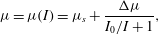 $$\begin{eqnarray}{\it\mu}={\it\mu}(I)={\it\mu}_{s}+\frac{{\rm\Delta}{\it\mu}}{I_{0}/I+1},\end{eqnarray}$$
where the dependence on the inertial number
 $I$
is scaled by a parameter
 $I_{0}$
and a friction constant
 ${\rm\Delta}{\it\mu}={\it\mu}_{d}-{\it\mu}_{s}$
with
 ${\it\mu}_{d}$
being known as the dynamic friction constant. In the notation introduced in this paper the inertial number is
 $$\begin{eqnarray}I=\frac{2d\Vert \unicode[STIX]{x1D63F}\Vert }{\sqrt{p/{\it\rho}}},\end{eqnarray}$$
which is equivalent to the definitions used by GDR-MiDi (2004) and Jop et al. (Reference Jop, Forterre and Pouliquen2006). The factor two arises from the use of the classical definition of the strain-rate tensor (2.1). The inertial number has the intuitive property that for higher values of
 $I$
the bulk shearing happens at a faster rate than the microscopic rearrangements and vice versa for low values. In the limit as
 $I\rightarrow \infty$
the friction
 ${\it\mu}(I)\rightarrow {\it\mu}_{d}$
, while
 ${\it\mu}(I)\rightarrow {\it\mu}_{s}$
as
 $I\rightarrow 0$
. Substituting the constitutive law (2.5)–(2.9) into (2.4), the momentum balance for the granular material can be written as
 $$\begin{eqnarray}\partial _{t}u_{i}+u_{j}\partial _{j}u_{i}=\partial _{j}\left[\frac{{\it\mu}(I)\check{p}}{\Vert \unicode[STIX]{x1D63F}\Vert }\unicode[STIX]{x1D60B}_{ij}\right]-\partial _{i}\check{p}+g_{i},\end{eqnarray}$$
where rescaled pressure
 $\check{p}$
is defined as
 $\check{p}=p/({\it\rho}{\it\phi})$
. Note that this scaling is motivated purely as a way of simplifying the governing equations, rather than as a formal non-dimensionalization of the variables. Dropping the superposed checks for simplicity, the corresponding inertial number with this rescaled pressure is therefore
 $$\begin{eqnarray}I=\frac{2d\Vert \unicode[STIX]{x1D63F}\Vert }{\sqrt{{\it\phi}p}}.\end{eqnarray}$$
The mass and momentum balances, (2.3) and (2.10), have a strong resemblance to the incompressible Navier–Stokes equations. Instead of having a constant viscosity, as in a Newtonian fluid, the dissipative terms are dependent on both the pressure and local deformation rate.
2.2. Expansion of the dissipative terms
In order to linearize the system of equations it is useful to expand the dissipative terms in (2.10) using the product rule, i.e.
 $$\begin{eqnarray}\partial _{j}\left[\frac{{\it\mu}p}{\Vert \unicode[STIX]{x1D63F}\Vert }\unicode[STIX]{x1D60B}_{ij}\right]=\frac{{\it\mu}p}{\Vert \unicode[STIX]{x1D63F}\Vert }\partial _{j}\unicode[STIX]{x1D60B}_{ij}+\frac{{\it\mu}}{\Vert \unicode[STIX]{x1D63F}\Vert }\unicode[STIX]{x1D60B}_{ij}\partial _{j}p+\frac{p}{\Vert \unicode[STIX]{x1D63F}\Vert }\unicode[STIX]{x1D60B}_{ij}\partial _{j}{\it\mu}+{\it\mu}p\unicode[STIX]{x1D60B}_{ij}\partial _{j}\Vert \unicode[STIX]{x1D63F}\Vert ^{-1}.\end{eqnarray}$$
Using incompressibility (2.3) the first term on the right-hand side reduces to
 $$\begin{eqnarray}\partial _{j}\unicode[STIX]{x1D60B}_{ij}=\partial _{jj}u_{i}/2,\end{eqnarray}$$
i.e. the Laplacian of
 $u_{i}$
. Due to the definition of the inertial number (2.11) it follows that
 $$\begin{eqnarray}\partial _{j}{\it\mu}(I)={\it\mu}^{\prime }(I)\left[\partial _{j}p\partial _{p}I+\partial _{j}\Vert \unicode[STIX]{x1D63F}\Vert \partial _{\Vert \unicode[STIX]{x1D63F}\Vert }I\right],\end{eqnarray}$$
where the derivative of the effective friction for the case of Jop et al.’s (Reference Jop, Forterre and Pouliquen2006) law (2.8) is
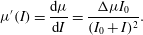 $$\begin{eqnarray}{\it\mu}^{\prime }(I)=\frac{\text{d}{\it\mu}}{\text{d}I}=\frac{{\rm\Delta}{\it\mu}I_{0}}{(I_{0}+I)^{2}}.\end{eqnarray}$$
This captures the increasing nature of the
 ${\it\mu}(I)$
curve (since
 ${\it\mu}^{\prime }\geqslant 0$
). Using the definition of the inertial parameter (2.11) it is then possible to calculate the derivative with respect to the pressure
 $$\begin{eqnarray}\partial _{p}I=-d\Vert \unicode[STIX]{x1D63F}\Vert ({\it\phi}p)^{-3/2}{\it\phi}=-\frac{I}{2p}\end{eqnarray}$$
and the second invariant of the strain rate
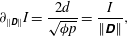 $$\begin{eqnarray}\partial _{\Vert \unicode[STIX]{x1D63F}\Vert }I=\frac{2d}{\sqrt{{\it\phi}p}}=\frac{I}{\Vert \unicode[STIX]{x1D63F}\Vert },\end{eqnarray}$$
which are needed to evaluate (2.14). Finally, the derivative of the strain-rate invariant is expanded as
 $$\begin{eqnarray}\partial _{j}\Vert \unicode[STIX]{x1D63F}\Vert =\partial _{j}\sqrt{\frac{1}{2}\mathop{\sum }_{k,l=1}^{2}(\unicode[STIX]{x1D60B}_{kl})^{2}}=\frac{1}{2}\left[\frac{1}{2}\mathop{\sum }_{k,l=1}^{2}(\unicode[STIX]{x1D60B}_{kl})^{2}\right]^{-1/2}\mathop{\sum }_{k,l=1}^{2}\unicode[STIX]{x1D60B}_{kl}\partial _{j}\unicode[STIX]{x1D60B}_{kl},\end{eqnarray}$$
where the summation has been written explicitly (cf. (2.2)). The expression can be simplified by defining a normalized strain-rate tensor
 $$\begin{eqnarray}\unicode[STIX]{x1D608}_{ij}=\frac{\unicode[STIX]{x1D60B}_{ij}}{\Vert \unicode[STIX]{x1D63F}\Vert },\end{eqnarray}$$
to show that
 $\partial _{j}\Vert \unicode[STIX]{x1D63F}\Vert =\unicode[STIX]{x1D608}_{kl}\partial _{j}\unicode[STIX]{x1D60B}_{kl}/2$
. Substituting for the strain rate
 $\unicode[STIX]{x1D60B}_{kl}$
and using the property that
 $\unicode[STIX]{x1D63C}$
is symmetric, the
 $\{1,2\}$
and
 $\{2,1\}$
components can be combined to show that (2.18) reduces to
 $$\begin{eqnarray}\partial _{j}\Vert \unicode[STIX]{x1D63F}\Vert ={\textstyle \frac{1}{2}}\unicode[STIX]{x1D608}_{kl}\partial _{j}\partial _{l}u_{k},\end{eqnarray}$$
determining the derivative in (2.14). In addition, it follows that the last term in (2.12) can be written as
 $$\begin{eqnarray}{\it\mu}p\unicode[STIX]{x1D60B}_{ij}\partial _{j}\Vert \unicode[STIX]{x1D63F}\Vert ^{-1}=-\frac{{\it\mu}p}{2\Vert \unicode[STIX]{x1D63F}\Vert }\unicode[STIX]{x1D608}_{ij}\unicode[STIX]{x1D608}_{kl}\partial _{j}\partial _{l}u_{k}.\end{eqnarray}$$
Substituting the expansions (2.13)–(2.21) into (2.12) implies that the dissipative term is
 $$\begin{eqnarray}\partial _{j}\left[\frac{{\it\mu}p}{\Vert \unicode[STIX]{x1D63F}\Vert }\unicode[STIX]{x1D60B}_{ij}\right]=\frac{{\it\mu}p}{2\Vert \unicode[STIX]{x1D63F}\Vert }\partial _{jj}u_{i}+\frac{{\it\mu}p}{2\Vert \unicode[STIX]{x1D63F}\Vert }[{\it\nu}-1]\unicode[STIX]{x1D608}_{ij}\unicode[STIX]{x1D608}_{kl}\partial _{j}\partial _{l}u_{k}+{\it\mu}[1-{\it\nu}/2]\unicode[STIX]{x1D608}_{ij}\partial _{j}p,\end{eqnarray}$$
where
 $$\begin{eqnarray}{\it\nu}=\frac{I{\it\mu}^{\prime }(I)}{{\it\mu}(I)}\end{eqnarray}$$
is a function of the inertial number.
2.3. Linearization and taking the principal part
It is assumed that there is a base state solution
 $(\boldsymbol{u}^{0},p^{0})$
that exactly satisfies the mass and momentum balance equations (2.3) and (2.10). The velocity and pressure are then perturbed about the base state, i.e.
 $$\begin{eqnarray}\boldsymbol{u}=\boldsymbol{u}^{0}+\hat{\boldsymbol{u}},\quad p=p^{0}+\hat{p},\end{eqnarray}$$
where
 $(\hat{\boldsymbol{u}},\hat{p})$
are small perturbations. In order to show ill-posedness of the system of equations, we are interested in the stability of the system in the high-wavenumber limit. This can be determined by taking the principal part of the linearized equations (Leray Reference Leray1953), i.e. we retain only the highest order derivatives of each perturbed field with respect to each variable. In particular, the viscous terms in (2.10) have already been expanded in (2.22) to identify that the highest order spatial derivatives of
 $\hat{\boldsymbol{u}}$
are second-order, while the highest spatial derivatives of
 $\hat{p}$
are first-order. It follows that in (2.10) the momentum transport terms
 $u_{j}\partial _{j}u_{i}$
can be neglected compared to the viscous terms, because they involve only first-order spatial derivatives. Similarly, assuming that
 $\partial _{j}\partial _{l}u_{k}^{0}$
and
 $\partial _{j}p^{0}$
are non-zero in the base state, the coefficients in (2.22) will generate a large number of terms on linearization. Crucially, however, these terms scale either with the pressure perturbations or with the first-order derivatives of the perturbed velocity, both of which can be neglected compared to the largest derivative terms in (2.22). Taking the principal part of the linearized equations therefore implies that the mass and momentum balances (2.3) and (2.10) are
 $$\begin{eqnarray}\displaystyle & \partial _{j}\hat{u} _{j}=0, & \displaystyle\end{eqnarray}$$
 $$\begin{eqnarray}\displaystyle & \partial _{t}\hat{u} _{i}={\it\eta}^{0}\left[\partial _{jj}\hat{u} _{i}-r\unicode[STIX]{x1D608}_{ij}\unicode[STIX]{x1D608}_{kl}\partial _{j}\partial _{l}\hat{u} _{k}\right]+\left[q\unicode[STIX]{x1D608}_{ij}\partial _{j}-\partial _{i}\right]\hat{p}, & \displaystyle\end{eqnarray}$$
 $\unicode[STIX]{x1D63F}$
, the normalized strain rate
 $\unicode[STIX]{x1D63C}$
, the inertial number
 $I$
and the coefficients
 $$\begin{eqnarray}{\it\eta}^{0}=\frac{{\it\mu}p^{0}}{2\Vert \unicode[STIX]{x1D63F}\Vert },\quad q={\it\mu}(1-{\it\nu}/2),\quad r=1-{\it\nu},\end{eqnarray}$$
are determined from the base state. Although the base state varies spatially, the values of the coefficients are treated as being locally constant, because in the high-wavenumber limit the base state appears frozen relative to the length scale of variations of the perturbation (Schmid & Henningson Reference Schmid and Henningson2001). Since the coefficients in (2.26) are constant, the governing equations (2.25) and (2.26) admit normal mode solutions of the form
 $$\begin{eqnarray}\left[\begin{array}{@{}c@{}}\hat{\boldsymbol{u}}(\boldsymbol{x},t)\\ \hat{p}(\boldsymbol{x},t)\end{array}\right]=\text{exp}(\text{i}{\bf\xi}\boldsymbol{\cdot }\boldsymbol{x}+{\it\lambda}t)\left[\begin{array}{@{}c@{}}\tilde{\boldsymbol{u}}\\ \tilde{p}\end{array}\right],\end{eqnarray}$$
where
 $\tilde{\boldsymbol{u}}$
and
 $\tilde{p}$
are constants,
 ${\bf\xi}$
is a real wavevector, ‘
 $\boldsymbol{\cdot }$
’ is the dot product and the growth rate
 ${\it\lambda}$
is anticipated to depend on the wavevector and flow properties. Ill-posedness corresponds to the case in which the growth rate tends to infinity in the high-wavenumber limit. Otherwise the equations are well-posed. Note that this local temporal stability analysis in the high-wavenumber limit has the advantage that it is not tied to a specific base state, and so the results are general. As such, the analysis can be applied across a whole flow, with varying properties, and irrespective of boundary effects, to determine regions of ill-posedness.
Note that in a usual linear stability analysis the governing equations are linearized about a known base state and solutions are sought for the growth rate of the perturbation. For base states with spatial gradients, standard analysis (valid for all wavenumbers) would usually require us to calculate the growth rates numerically, and the boundary conditions would also filter the range of acceptable modes. This not only significantly complicates the analysis, but, if it needs to be solved numerically, the wavenumbers must be discretized, which makes it much more difficult to infer that they tend to infinity in the high-wavenumber limit and hence ill-posedness (Joseph & Saut Reference Joseph and Saut1990). In contrast, in the approach used here, gradients of the base state are infinitely small compared to those of the perturbation, so they can be neglected. In addition the perturbation boundary conditions can always be satisfied, because the wavenumber can, if necessary, always be multiplied by an arbitrary factor and it is still infinite. Our approach is therefore much simpler than a standard linear stability analysis, but has the advantage that it yields a very clear and concise asymptotic result.
2.4. The eigenvalue problem
Substitution of the normal mode solution (2.28) into the linearized equations (2.25) and (2.26) results in the generalized eigenvalue problem
 $$\begin{eqnarray}\displaystyle & \text{i}{\it\xi}_{j}\tilde{u} _{j}=0 & \displaystyle\end{eqnarray}$$
 $$\begin{eqnarray}\displaystyle & {\it\lambda}\tilde{u} _{i}={\it\eta}^{0}\left[-|{\bf\xi}|^{2}\tilde{u} _{i}+r\unicode[STIX]{x1D608}_{ij}{\it\xi}_{j}\unicode[STIX]{x1D608}_{kl}{\it\xi}_{l}\tilde{u} _{k}\right]+\text{i}\tilde{p}[q\unicode[STIX]{x1D608}_{ij}{\it\xi}_{j}-{\it\xi}_{i}]. & \displaystyle\end{eqnarray}$$
 $\tilde{p}$
to be solved for explicitly by taking the dot product of (2.30) with the wavevector
 ${\bf\xi}$
to give
 $$\begin{eqnarray}\tilde{p}=-\text{i}r{\it\eta}^{0}\left(\frac{\unicode[STIX]{x1D608}_{ij}{\it\xi}_{j}{\it\xi}_{i}\unicode[STIX]{x1D608}_{kl}{\it\xi}_{l}\tilde{u} _{k}}{|{\bf\xi}|^{2}-q\unicode[STIX]{x1D608}_{ij}{\it\xi}_{j}{\it\xi}_{i}}\right).\end{eqnarray}$$
Since the numerator in this expression is third-order in wavenumber and the denominator is second-order, the pressure perturbation constant scales linearly with wavenumber. It follows that all the terms on the right-hand side of (2.30) are second-order in wavenumber. Substituting the pressure constant (2.31) into (2.30) yields the eigenvalue problem
 $$\begin{eqnarray}\boldsymbol{L}\tilde{\boldsymbol{u}}={\it\lambda}\tilde{\boldsymbol{u}},\end{eqnarray}$$
where the operator
 $$\begin{eqnarray}\boldsymbol{L}={\it\eta}^{0}\left[r\left(\unicode[STIX]{x1D63C}{\bf\xi}-\frac{(\unicode[STIX]{x1D63C}{\bf\xi}\boldsymbol{\cdot }{\bf\xi})({\bf\xi}-q\unicode[STIX]{x1D63C}{\bf\xi})}{|{\bf\xi}|^{2}-q({\bf\xi}\boldsymbol{\cdot }\unicode[STIX]{x1D63C}{\bf\xi})}\right)(\unicode[STIX]{x1D63C}{\bf\xi})^{\text{T}}-|{\bf\xi}|^{2}\pmb{{\it 1}}\right].\end{eqnarray}$$
2.5. Determining the growth rate
The eigenvalue
 ${\it\lambda}$
is recovered by finding a permissible eigenvector. Due to the orthogonality of the wavevector and velocity (2.29), and the strict restriction to two-dimensional flows, only eigenvectors proportional to
 ${\bf\xi}^{\bot }=({\it\xi}_{2},-{\it\xi}_{1})$
can be accepted. It is readily checked that
 ${\bf\xi}\boldsymbol{\cdot }\boldsymbol{L}{\bf\xi}^{\bot }=0$
, so that
 ${\bf\xi}^{\bot }$
is indeed an eigenvector. Substituting
 ${\bf\xi}^{\bot }$
for
 $\tilde{\boldsymbol{u}}$
in the eigenvalue (2.32) and taking the dot product with
 ${\bf\xi}^{\bot }$
yields
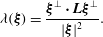 $$\begin{eqnarray}{\it\lambda}({\bf\xi})=\frac{{\bf\xi}^{\bot }\boldsymbol{\cdot }\boldsymbol{L}{\bf\xi}^{\bot }}{|{\bf\xi}|^{2}}.\end{eqnarray}$$
Substitution of the operator
 $\boldsymbol{L}$
from (2.33) then gives the growth rate
 $$\begin{eqnarray}{\it\lambda}({\bf\xi})={\it\eta}^{0}\left(\frac{q\left|{\bf\xi}\right|^{2}({\bf\xi}\boldsymbol{\cdot }\unicode[STIX]{x1D63C}{\bf\xi})-\left|{\bf\xi}\right|^{4}+r({\bf\xi}^{\bot }\boldsymbol{\cdot }\unicode[STIX]{x1D63C}{\bf\xi})^{2}}{\left|{\bf\xi}\right|^{2}-q({\bf\xi}\boldsymbol{\cdot }\unicode[STIX]{x1D63C}{\bf\xi})}\right).\end{eqnarray}$$
It is important to note that this expression scales as
 $|{\bf\xi}|^{2}$
. This means that if
 ${\it\lambda}$
is positive, there will be growth of perturbations with an ever larger rate for higher wavenumbers (ill-posedness). Conversely, if the growth rate is negative, all perturbations will decay exponentially and the system is well-posed.
Considering typical parameter values from the literature (Jop et al.
Reference Jop, Forterre and Pouliquen2005) along with the physical argument that higher deformation implies more dissipation, it is observed that
 ${\rm\Delta}{\it\mu}>0$
and
 ${\it\mu}_{d}<1$
. Such consideration gives
 $q<1$
, and as
 $\Vert \unicode[STIX]{x1D63C}\Vert =1$
the denominator in (2.35) is always positive. The sign of the growth rate is therefore determined by the sign of the numerator
 $$\begin{eqnarray}N=q\left|{\bf\xi}\right|^{2}({\bf\xi}\boldsymbol{\cdot }\unicode[STIX]{x1D63C}{\bf\xi})-\left|{\bf\xi}\right|^{4}+r({\bf\xi}^{\bot }\boldsymbol{\cdot }\unicode[STIX]{x1D63C}{\bf\xi})^{2}.\end{eqnarray}$$
Determining the sign of (2.36) is greatly helped by the properties of
 $\unicode[STIX]{x1D63C}$
. In addition to its normalization, it is also the case that
 $\text{tr}\,\unicode[STIX]{x1D63C}=0$
due to the definition of the strain-rate tensor (2.1). These properties imply that any permissible
 $\unicode[STIX]{x1D63C}$
is orthogonally similar to
 $$\begin{eqnarray}\tilde{\unicode[STIX]{x1D63C}}=\left[\begin{array}{@{}cc@{}}1 & 0\\ 0 & -1\end{array}\right]\end{eqnarray}$$
and so any result found with this is true for all systems given an appropriate linear coordinate transformation. The choice of this particular form allows for some convenient factorizations as will be demonstrated below. Assuming that the wavevector in this system is
 $\tilde{{\bf\xi}}$
, it follows that when (2.37) is substituted into (2.36) and divided by
 $\tilde{{\it\xi}}_{2}^{4}$
the condition on the numerator is
 $$\begin{eqnarray}{\tilde{N}}=(q-1)\left(\frac{\tilde{{\it\xi}}_{1}}{\tilde{{\it\xi}}_{2}}\right)^{4}+(4r-2)\left(\frac{\tilde{{\it\xi}}_{1}}{\tilde{{\it\xi}}_{2}}\right)^{2}+(-q-1),\end{eqnarray}$$
i.e. a quartic of the perturbation direction,
 $\tilde{{\it\xi}}_{1}/\tilde{{\it\xi}}_{2}$
. The sign of
 ${\tilde{N}}$
, and thus the growth rate, is then dependent on the model parameters
 $q$
and
 $r$
, defined in (2.28), and the perturbation direction. Considering first the neutral stability case
 ${\tilde{N}}=0$
gives directions for each of the four roots
 $$\begin{eqnarray}\frac{\tilde{{\it\xi}}_{1}}{\tilde{{\it\xi}}_{2}}=\pm \left(\frac{1-2r}{q-1}\pm \frac{\sqrt{4r^{2}-4r+q^{2}}}{q-1}\right)^{1/2},\end{eqnarray}$$
where the four distinct combinations of
 $\pm$
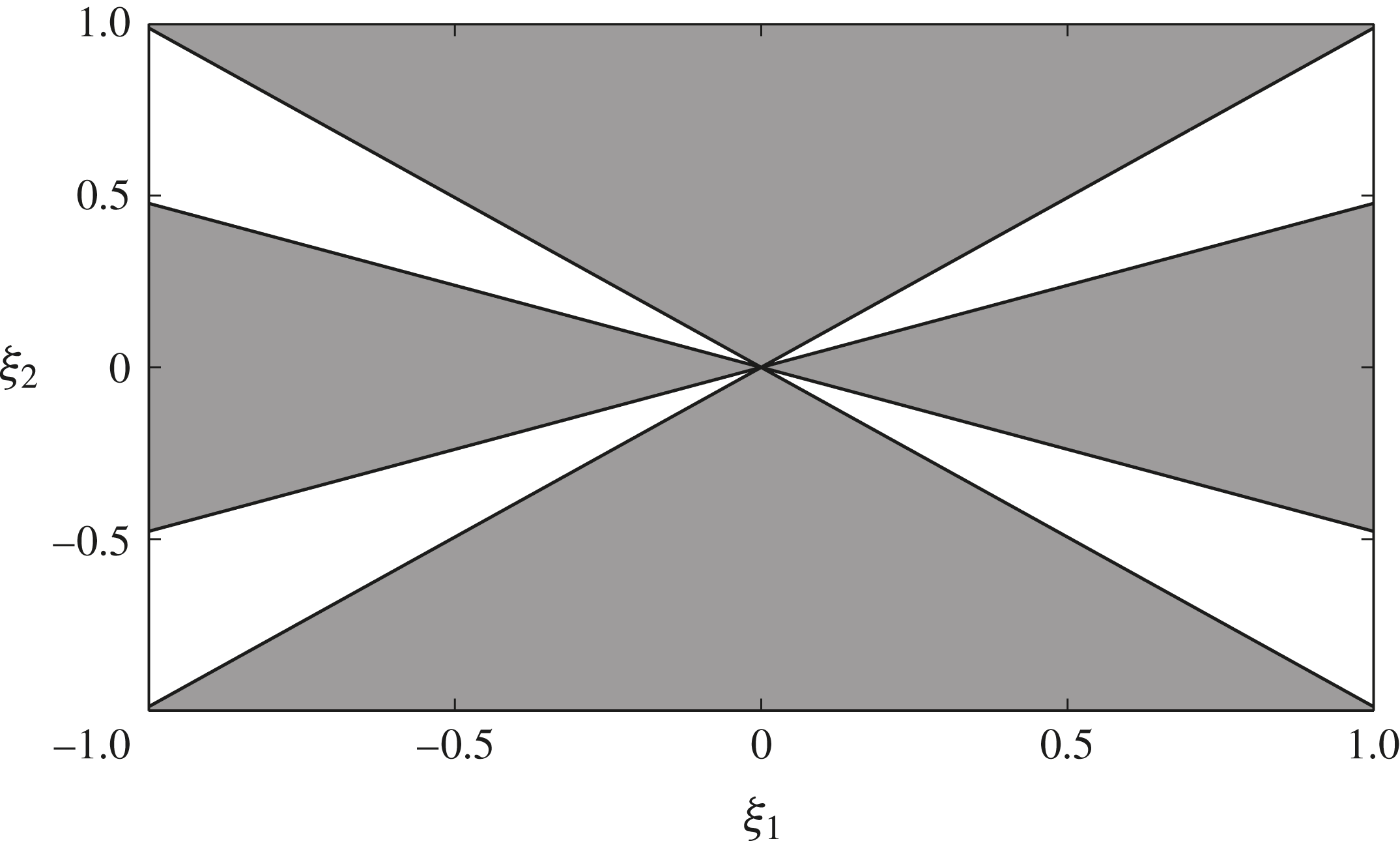
are taken. The sign in the regions between these determines the range of directions for which the perturbations grow or decay, as shown in figure 1. The numerator
 ${\tilde{N}}$
is negative in the grey shaded regions, indicating that the wavevectors oriented in these directions are well-posed. However, in the unshaded regions
 ${\tilde{N}}$
is positive and the wavevectors will grow infinitely quickly in the high-wavenumber limit (ill-posedness). In order for such ill-posed directions to exist, the roots (2.39) must be real. This then sets the inequalities
 $$\begin{eqnarray}\displaystyle & 4r^{2}-4r+q^{2}>0, & \displaystyle\end{eqnarray}$$
 $$\begin{eqnarray}\displaystyle & 1-2r<0, & \displaystyle\end{eqnarray}$$
 $q<1$
. Using the definition of
 $r$
, in (2.27), it follows that (2.41) is equivalent to
 ${\it\nu}<1/2$
, where
 ${\it\nu}$
is given by (2.8) and (2.23) as
 $$\begin{eqnarray}{\it\nu}=\frac{{\rm\Delta}{\it\mu}(I_{0}/I)}{(1+I_{0}/I)({\it\mu}_{s}I_{0}/I+{\it\mu}_{d})}.\end{eqnarray}$$
This is equal to zero in the limits when
 $I\rightarrow 0$
and
 $I\rightarrow \infty$
. For the parameters given in table 1, the maximum value of
 ${\it\nu}\simeq 0.1288$
, so (2.41) is always satisfied. Using (2.27) the remaining condition for ill-posedness (2.40) can be expressed as
 $$\begin{eqnarray}4{\it\nu}^{2}-4{\it\nu}+{\it\mu}^{2}(1-{\it\nu}/2)^{2}>0.\end{eqnarray}$$
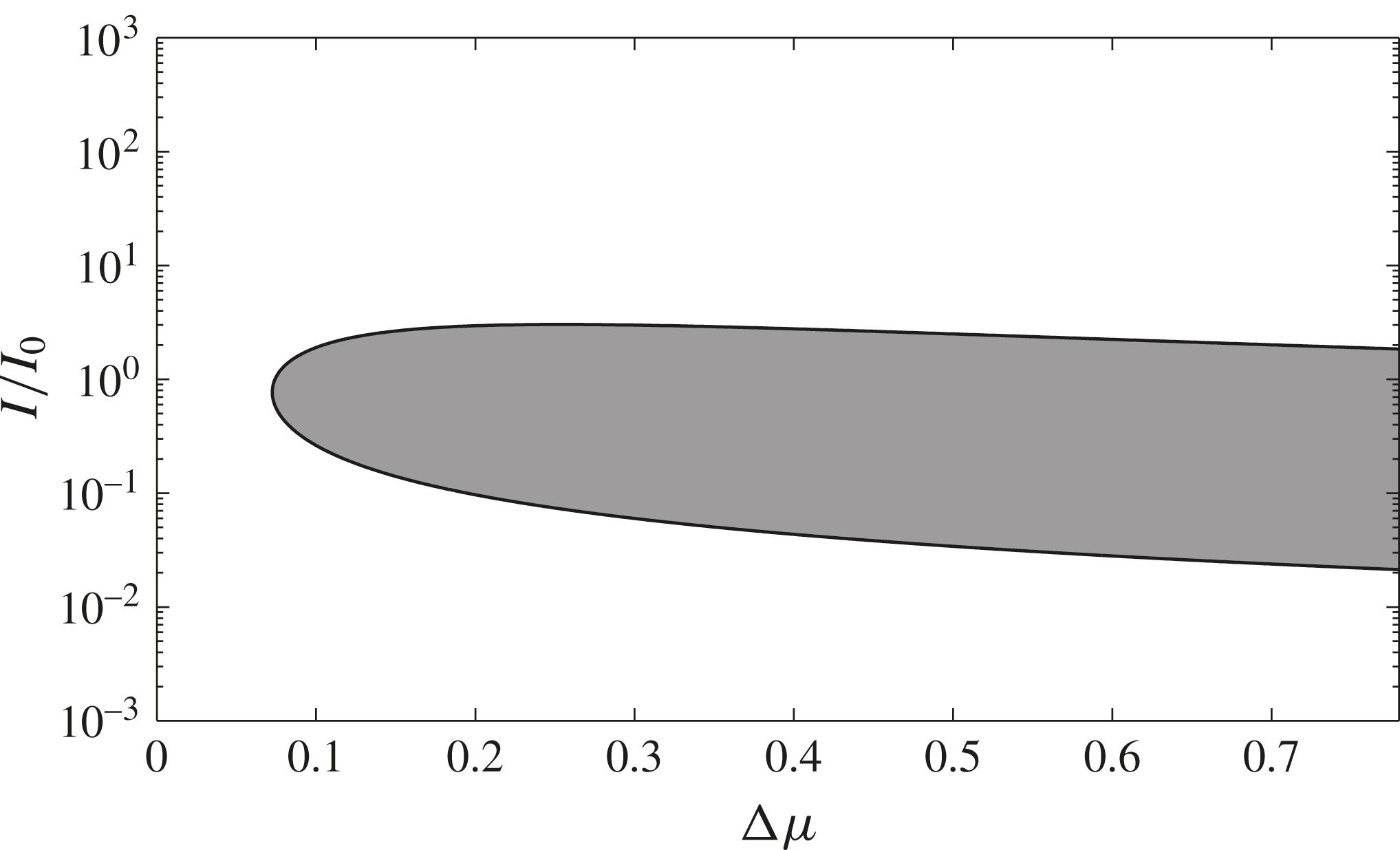
Figure 2 shows a semi-logarithmic plot of this condition as a function of
 ${\rm\Delta}{\it\mu}$
and
 $I/I_{0}$
for the value of
 ${\it\mu}_{s}$
given in table 1. The white region, outside the neutral stability curve, is the set of flows for which there exist perturbation directions with an unbounded positive growth rate (ill-posedness). Conversely, for flows with parameters in the shaded region, all perturbations are guaranteed to decay, so the system is well-posed. It is reassuring that the original result for a pure Coulomb material (Schaeffer Reference Schaeffer1987) is recovered here, i.e. when
 ${\rm\Delta}{\it\mu}=0$
the equations are always ill-posed regardless of the local value of
 $I$
. For values of
 ${\rm\Delta}{\it\mu}$
above a critical level the rate dependence of the
 ${\it\mu}(I)$
-rheology is sufficient to make the equations well-posed over a large intermediate range of
 $I/I_{0}$
that spans almost two orders of magnitude. However, for sufficiently large or sufficiently small values of
 $I/I_{0}$
the equations are ill-posed. The fact that the
 ${\it\mu}(I)$
-rheology is ill-posed for high and low inertial numbers is far from obvious from casual inspection of the equations, so the ill-posedness criterion (2.43) is a very useful and important result.
A stability diagram showing the sign of the numerator
 ${\tilde{N}}$
for different wavevectors
 ${\bf\xi}=({\it\xi}_{1},{\it\xi}_{2})$
in the case
 $\tilde{A}$
given by (2.37) and parameters
 $I_{0}=0.279$
,
 ${\rm\Delta}{\it\mu}=0.26$
and
 ${\it\mu}_{s}=0.383$
. The grey shaded regions correspond to negative
 ${\tilde{N}}$
, which implies that these directions are well-posed. The white regions are where
 ${\tilde{N}}$
is positive and the perturbation directions are ill-posed. The value of
 $I=100$
is chosen to ensure that ill-posed directions exist in this case.
The ill-posed region (white) and well-posed region (grey) with neutral stability curve (black) for the general result (2.43) as a function of the inertial number
 $I/I_{0}$
and the friction constant
 ${\rm\Delta}{\it\mu}$
. This diagram holds for all permissible base states
 $\unicode[STIX]{x1D63C}$
with
 ${\it\mu}_{s}=0.383$
and for all other material parameters.
Parameter values used in this paper unless specified otherwise.

Since (2.43) is not dependent on a specific base state, it provides a universal criterion for ill-posedness of the
 ${\it\mu}(I)$
-rheology that can be applied to any two-dimensional flow. For steady-uniform chute flows, the inertial number
 $I$
is constant through the depth of the avalanche. It varies with the slope inclination angle, from zero at the minimum angle for steady-uniform flow to infinity as the maximum angle for steady-uniform flow is approached (GDR-MiDi 2004; Jop et al.
Reference Jop, Forterre and Pouliquen2005; Gray & Edwards Reference Gray and Edwards2014). It follows that chute flows can be modelled with the
 ${\it\mu}(I)$
-rheology provided that the inclination angle is not too high or too low. However, many commonly occurring practical granular flows, such as the column collapses (Lagrée et al.
Reference Lagrée, Staron and Popinet2011), formation of heaps, silo flow (Kamrin Reference Kamrin2010; Staron et al.
Reference Staron, Lagrée and Popinet2012) and flows in rotating drums, are problematic, since they will have a large quasi-static body of grains, where
 $I/I_{0}\rightarrow 0$
, and/or low-density collisional regions, where
 $I/I_{0}\rightarrow \infty$
. In these regions the governing equations will be ill-posed.
The implications of this type of ill-posedness are summarized for a selection of typical problems by Joseph & Saut (Reference Joseph and Saut1990). As the growth rate (2.35) is unbounded for short wavelengths, numerical integration of these equations will lead to a catastrophic blow-up of any perturbations if the parameters are in the ill-posed region. Furthermore, due to the quadratic dependence on wavenumber, shorter wavelength disturbances will be amplified more strongly and so calculations will fail more readily with increased spatial resolution. A simple practical example of this is provided by the segregation-induced fingering model of Woodhouse et al. (Reference Woodhouse, Thornton, Johnson, Kokelaar and Gray2012). The results at any fixed grid resolution look reasonably good. However, on refining the grid resolution the number of fingers increases, since their width is controlled by the numerical viscosity. Continued refinement of the grid does not help, as the numerical results do not converge to a well-defined solution with a fixed number of fingers. Similar behaviour is also observed in a granular model for the breakup of sea-ice (Gray Reference Gray1999).
Knowing that a system of equations is ill-posed is very useful, because it is a clear indication that important physics is missing in the mathematical model. In this case it is likely that in the quasi-static elastic limit (Campbell Reference Campbell2002) force chains (Howell, Behringer & Veje Reference Howell, Behringer and Veje1999), the contact fabric (Toiya, Stambaugh & Losert Reference Toiya, Stambaugh and Losert2004; Sun & Sundaresan Reference Sun and Sundaresan2011) and shear bands (Wu, Bauer & Kolymbas Reference Wu, Bauer and Kolymbas1996; Ehlers & Volk Reference Ehlers and Volk1998) play an important role. In contrast, for large inertial numbers there is a transition to a low-density granular gas dominated by particle collisions (Jenkins & Savage Reference Jenkins and Savage1983; Goldhirsch Reference Goldhirsch2003). It does not appear to be possible to include these effects by way of a minor modification to the
 ${\it\mu}(I)$
-rheology. For instance, the extended friction law of Pouliquen & Forterre (Reference Pouliquen and Forterre2002) suggests that the effective friction
 ${\it\mu}(I)$
is a decreasing function of
 $I$
for small inertial numbers below a certain threshold. A simplified version of this can be achieved by assuming that
 ${\it\mu}_{s}>{\it\mu}_{d}$
in the above analysis. It is again the case that
 $q<1$
and
 $1-2r<0$
, so the same ill-posedness criterion (2.43) applies. In this case, however,
 ${\it\mu}^{\prime }(I)$
is negative, because
 ${\it\mu}(I)$
is a decreasing function, and hence
 ${\it\nu}$
is negative. Substituting this into (2.43) implies that the resulting model is always ill-posed. More radical changes to the
 ${\it\mu}(I)$
-rheology are therefore necessary if it is to be able to transition between flow regimes.
3. Numerical validation
Theoretical results on the ill-posedness of the equations might, perhaps understandably, struggle to gain wide acceptance when there is such strong evidence pointing towards the
 ${\it\mu}(I)$
-rheology being a good constitutive law for the dense inertial regime. It is important to stress that our results do not contradict this, since we have shown that the equations are well-posed for a large and precisely defined intermediate region of parameter space. The model is, however, ill-posed outside this region, which will now be demonstrated numerically for a specific case.
3.1. Governing equations and the base state
The incompressible constraint (2.3) and the momentum balance equation (2.10) can be written in strong-conservation, compact form as
 $$\begin{eqnarray}\displaystyle & \boldsymbol{{\rm\nabla}}\boldsymbol{\cdot }\boldsymbol{u}=0, & \displaystyle\end{eqnarray}$$
 $$\begin{eqnarray}\displaystyle & \partial _{t}\boldsymbol{u}+\boldsymbol{{\rm\nabla}}\boldsymbol{\cdot }(\boldsymbol{u}\otimes \boldsymbol{u})=-\boldsymbol{{\rm\nabla}}p+\boldsymbol{{\rm\nabla}}\boldsymbol{\cdot }(2\,{\it\eta}\,\unicode[STIX]{x1D63F})+\boldsymbol{g}, & \displaystyle\end{eqnarray}$$
 ${\it\eta}$
is given by
 $$\begin{eqnarray}{\it\eta}\equiv \frac{{\it\mu}(I)\,p}{2\,\Vert \unicode[STIX]{x1D63F}\Vert },\end{eqnarray}$$
and is not evaluated in the base state as in (2.27). This is equivalent to the definition of Andreotti, Forterre & Pouliquen (Reference Andreotti, Forterre and Pouliquen2013) except they formulated it in terms of the second invariant of the shear-rate tensor,
 $|\dot{{\it\gamma}}|=2\Vert \unicode[STIX]{x1D63F}\Vert$
. Note that the density has been completely eliminated from the problem by scaling the pressure just after (2.10). The fully nonlinear evolution of the equations is calculated relative to simple shear, i.e. it is assumed that the base state is
 $$\begin{eqnarray}\boldsymbol{u}^{0}=(x_{2},0),\quad p^{0}=\text{const.},\quad \text{and}\quad \boldsymbol{g}=\mathbf{0},\end{eqnarray}$$
where the coordinate
 $\boldsymbol{x}=(x_{1},x_{2})$
. A positive non-zero value of
 $p^{0}$
is used to avoid non-physical negative pressures and the inherent singularity in the inertial parameter (2.11) in the limit of zero pressure. The exact solution (3.4) has a linear shear profile with strain-rate invariant
 $\Vert \unicode[STIX]{x1D63F}\Vert =1/2$
and an inertial number
 $I$
that is constant and uniform throughout the flow. The normalized strain-rate tensor
 $$\begin{eqnarray}\unicode[STIX]{x1D63C}=\left[\begin{array}{@{}cc@{}}0 & 1\\ 1 & 0\end{array}\right]\end{eqnarray}$$
is also constant. The wavevector
 ${\bf\xi}$
and the normalized strain-rate
 $\unicode[STIX]{x1D63C}$
can be mapped to
 $\tilde{{\bf\xi}}$
and
 $\tilde{\unicode[STIX]{x1D63C}}$
, defined in (2.37), by applying an orthogonal transformation of the form
 $$\begin{eqnarray}\tilde{{\bf\xi}}=\unicode[STIX]{x1D64C}{\bf\xi}\quad \text{and}\quad \tilde{\unicode[STIX]{x1D63C}}=\unicode[STIX]{x1D64C}\unicode[STIX]{x1D63C}\unicode[STIX]{x1D64C}^{\text{T}}.\end{eqnarray}$$
In this case the orthogonal matrix
 $$\begin{eqnarray}\unicode[STIX]{x1D64C}=\frac{1}{\sqrt{2}}\left[\begin{array}{@{}cc@{}}1 & 1\\ 1 & -1\end{array}\right],\end{eqnarray}$$
which implies that the
 ${\bf\xi}$
and
 $\tilde{{\bf\xi}}$
coordinates are related by
 $$\begin{eqnarray}{\bf\xi}=\unicode[STIX]{x1D64C}^{\text{T}}\tilde{{\bf\xi}}=\left[\begin{array}{@{}c@{}}{\it\xi}_{1}\\ {\it\xi}_{2}\end{array}\right]=\frac{1}{\sqrt{2}}\left[\begin{array}{@{}c@{}}\tilde{{\it\xi}}_{1}+\tilde{{\it\xi}}_{2}\\ \tilde{{\it\xi}}_{1}-\tilde{{\it\xi}}_{2}\end{array}\right].\end{eqnarray}$$
Substituting the normalized strain-rate tensor (3.5) together with the wavevector (3.8) into the growth rate (2.35) yields precisely the same numerator (2.38) and ill-posedness condition (2.43) as in
 $\tilde{{\bf\xi}}$
coordinates. Since the growth rate
 ${\it\lambda}$
will be compared directly with that in the numerical simulations, the above analysis shows that it does not matter whether it is evaluated using
 ${\bf\xi}$
and
 $\unicode[STIX]{x1D63C}$
, or simply mapped back to
 $\tilde{{\bf\xi}}$
and
 $\tilde{\unicode[STIX]{x1D63C}}$
.
3.2. The numerical scheme
The system (3.1) and (3.2) is solved numerically using the finite volume method (see Ferziger & Perić Reference Ferziger and Perić2002) implemented in OpenFOAM®, an open-source computational fluid dynamics software package. The high-quality performance of this library has been demonstrated in the context of incompressible-flow stability analysis by several authors (e.g. Bohorquez et al.
Reference Bohorquez, Sanmiguel-Rojas, Sevilla, Jimenez-Gonzalez and Martínez-Bazán2011). Here a specific solver is detailed that computes the temporal evolution of nonlinear perturbations, adopting the approach proposed by Favero et al. (Reference Favero, Secchi, Cardozo and Jasak2010) for the direct numerical simulation of viscoelastic flows. Substituting for the velocity and pressure from (2.24), the nonlinear perturbation equations for
 $(\hat{\boldsymbol{u}},\hat{p})$
become
 $$\begin{eqnarray}\displaystyle & \boldsymbol{{\rm\nabla}}\boldsymbol{\cdot }\hat{\boldsymbol{u}}=0, & \displaystyle\end{eqnarray}$$
 $$\begin{eqnarray}\displaystyle & \partial _{t}\hat{\boldsymbol{u}}-\boldsymbol{{\rm\nabla}}\boldsymbol{\cdot }({\it\eta}\boldsymbol{{\rm\nabla}}\hat{\boldsymbol{u}})=-\boldsymbol{{\rm\nabla}}\hat{p}+\boldsymbol{{\rm\nabla}}\boldsymbol{\cdot }({\it\eta}\boldsymbol{{\rm\nabla}}\boldsymbol{u}^{0})+(\boldsymbol{{\rm\nabla}}\hat{\boldsymbol{u}}+\boldsymbol{{\rm\nabla}}\boldsymbol{u}^{0})\boldsymbol{\cdot }\boldsymbol{{\rm\nabla}}{\it\eta}, & \displaystyle\end{eqnarray}$$
 $\boldsymbol{{\rm\nabla}}\boldsymbol{\cdot }({\it\eta}\boldsymbol{{\rm\nabla}}^{\text{T}})$
and yield the last term on the right-hand side of (3.10). Recall that
 ${\it\eta}$
denotes the nonlinear viscosity defined in (3.3) and is evaluated with the full nonlinear pressure and velocity fields
 $p=\hat{p}+p_{0}$
and
 $u=\hat{u} +u_{0}$
, respectively. In order to compare the results with the linear stability analysis in § 2 the convective terms have been neglected. It has, however, been confirmed that these do not affect the results for the problem presented here. The main difference with respect to the Newtonian case with constant viscosity is that the last two terms on the right-hand side of (3.10) do not vanish, because the perturbed viscosity
 ${\it\eta}$
is not uniform during the development of the instabilities. These terms introduce additional numerical difficulties due to the coupling between components of the momentum balance equations. This is overcome by evaluating them as part of the correction term
 ${\bf\tau}_{corr}$
in Favero et al. (Reference Favero, Secchi, Cardozo and Jasak2010) owing to a decoupled approach in the inner PISO loop. At every time step, the outer loop was iterated whilst updating
 ${\it\eta}$
and
 ${\bf\tau}_{corr}$
until convergence; this eventually leads to a fully implicit scheme. Note that the present method differs from Lagrée et al. (Reference Lagrée, Staron and Popinet2011), who adopted an explicit scheme for the coupling terms. For further details on the numerical method, the reader is referred to Favero et al. (Reference Favero, Secchi, Cardozo and Jasak2010).
The discretization of the differential operators is implemented in OpenFOAM on a per-operator basis (Weller et al.
Reference Weller, Tabor, Jasak and Fureby1998). A second-order backward scheme is found to be preferable for the temporal derivative, and the Gauss theorem was employed to discretize the divergence, gradient and Laplacian operators, interpolating linearly the variables at the cell faces from the cell centroids; see Jasak (Reference Jasak1996) for details. As such, the method is second-order accurate in space and time. Periodic boundary conditions are then imposed at the geometrical level in a rectangular mesh. The pressure perturbation
 $\hat{p}$
is set to the constant value of zero at one cell in accordance with the initial conditions described below.
3.3. Initial and boundary conditions
The initial perturbations are taken to be combinations of sines and cosines. It is therefore useful to define a scaled wavevector
 $\boldsymbol{k}$
, where
 $$\begin{eqnarray}{\bf\xi}=2{\rm\pi}\boldsymbol{k}.\end{eqnarray}$$
In order to satisfy the condition that the velocity perturbation is perpendicular to the wavevector (2.29) the initial velocity vector is chosen to be proportional to
 $\boldsymbol{k}^{\bot }$
. Its maximum initial magnitude is small and is taken to be equal to
 ${\it\varepsilon}=1\times 10^{-7}~\text{m}~\text{s}^{-1}$
. Sinusoidal dependence is achieved by taking the imaginary part of (2.28) to give
 $$\begin{eqnarray}\hat{\boldsymbol{u}}(\boldsymbol{x},0)={\it\varepsilon}\sin (2{\rm\pi}\boldsymbol{k}\boldsymbol{\cdot }\boldsymbol{x})\frac{\boldsymbol{k}^{\bot }}{|\boldsymbol{k}|}.\end{eqnarray}$$
The corresponding initial pressure perturbation is calculated directly from (2.31) and is exactly out of phase with the velocity, i.e.
 $$\begin{eqnarray}\hat{p}(\boldsymbol{x},0)=-4{\rm\pi}{\it\varepsilon}r{\it\mu}p^{0}\frac{k_{1}k_{2}(k_{2}^{2}-k_{1}^{2})}{k_{1}^{2}+k_{2}^{2}-2qk_{1}k_{2}}\left(\frac{\cos \left(2{\rm\pi}\boldsymbol{k}\boldsymbol{\cdot }\boldsymbol{x}\right)}{\sqrt{k_{1}^{2}+k_{2}^{2}}}\right).\end{eqnarray}$$
When ill-posed directions exist, they exist for very low and very high values of
 $k_{1}/k_{2}$
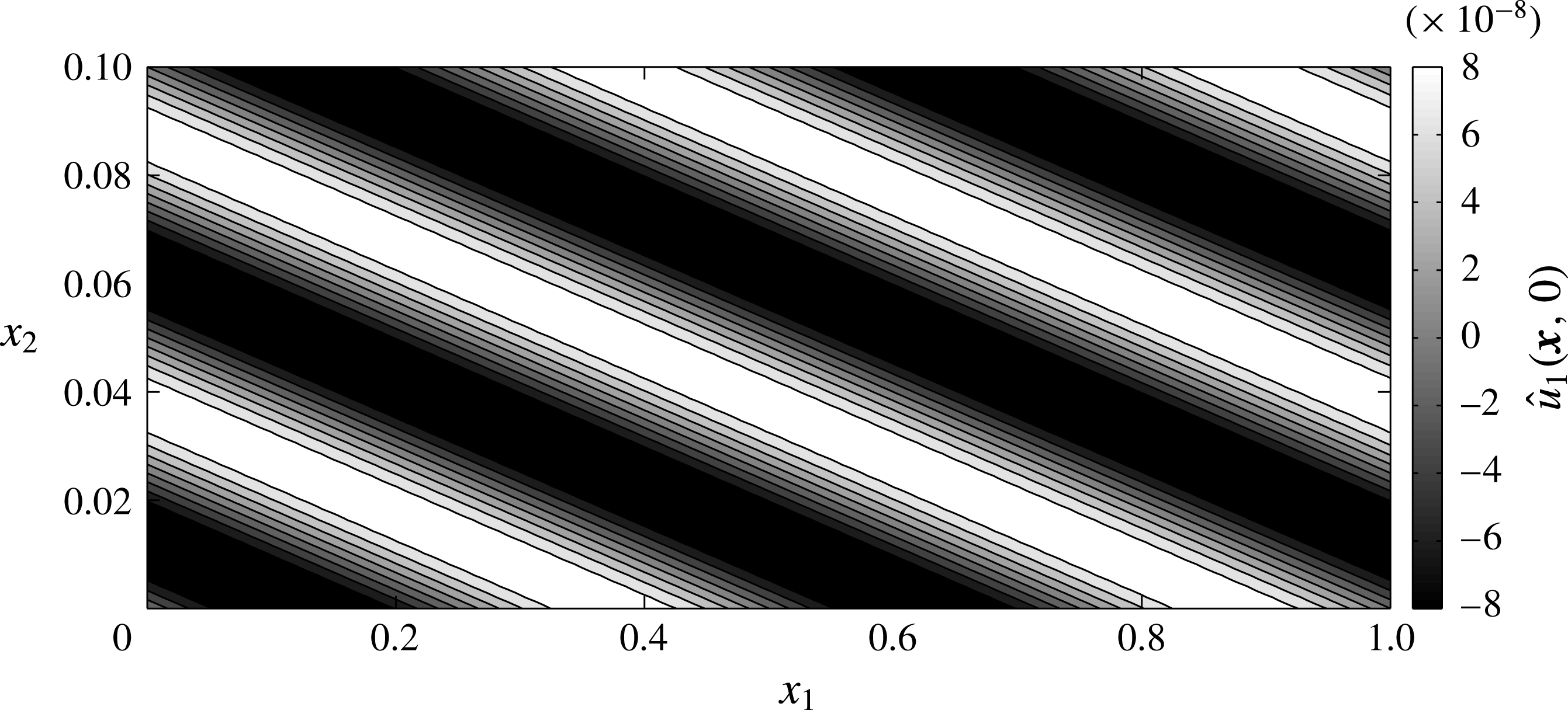
. A typical initial velocity perturbation that might lead to ill-posed results is illustrated in figure 3 for
 $k_{1}/k_{2}=1/10$
. This also shows why the factor of
 $2{\rm\pi}$
has been introduced in (3.11). By ensuring that the components of
 $k$
are integer values, and with a fixed integer ratio, the simulation domain can be rectangular and have doubly periodic boundaries. Wrapping of the
 $x_{1}$
and
 $x_{2}$
axes makes this domain representative of a region in the bulk of a flow for which the variation of the perturbation is dominant. Note that despite the base state velocity (3.4) not being periodic, periodic boundaries are still permissible as only its gradient appears in the simulated (3.9) and (3.10), which is a constant across the domain.
A typical initial velocity perturbation,
 $\hat{\boldsymbol{u}}(\boldsymbol{x},0)$
given by (3.12). Here, the
 $x_{1}$
component of the velocity field is shown for the parameters
 $\boldsymbol{k}=(2,20)$
and
 ${\it\varepsilon}=1\times 10^{-7}~\text{m}~\text{s}^{-1}$
.
3.4. Results
The perturbation equations (3.9) and (3.10) are solved numerically subject to the initial conditions (3.12) and (3.13) on a doubly periodic rectangular domain using the parameter values specified in table 1. Due to the assumed exponential form of the perturbations (2.28) the simulated growth rate can be recovered by taking the log of the perturbation and differentiating with respect to time, i.e.
 $$\begin{eqnarray}{\it\lambda}=\frac{\text{d}}{\text{d}t}(\ln \hat{\boldsymbol{u}}|_{\boldsymbol{x}_{p}}),\end{eqnarray}$$
where
 $\boldsymbol{x}_{p}$
is a fixed computation cell that is chosen such that the velocity perturbation (3.12) is maximal. This is equivalent to calculating the growth rate of the envelope of the perturbation, which is the most common method (see e.g. Theofilis Reference Theofilis2003, Reference Theofilis2011; Bohorquez et al.
Reference Bohorquez, Sanmiguel-Rojas, Sevilla, Jimenez-Gonzalez and Martínez-Bazán2011). The variance of this fitting is very low for early simulation times (while the magnitude of the perturbations is small) and the exponential growth is therefore confirmed. To ensure that the results are invariant, convergence studies were performed. Such studies consist of refinement of the time step
 ${\rm\Delta}t$
and computation cell size
 ${\rm\Delta}x_{i}$
until values of the growth rate were constant. As it is readily shown that the product
 $pt$
is an invariant of the governing equations, the time step was written in terms of the base state pressure. It is found that a sufficiently small time step is
 ${\rm\Delta}t=10^{-8}/p^{0}$
.
For the spatial discretization it was found that scaling the grid resolution with the perturbation wavenumber gives computational domains for which the dynamics can be most consistently compared. This scaling avoids issues caused by the inherent numerical viscosity due to digital truncation. For the simulations presented here, the perturbation is fixed in a direction (
 $k_{1}/k_{2}=1/10$
) predicted to lie in the ill-posed region, when it exists, and then the wavelength and parameter values are changed about this. It is therefore convenient to write the perturbations in the form
 $\boldsymbol{k}=(k,10k)$
, where
 $k$
is a positive integer. It was found from the convergence studies that setting
 ${\rm\Delta}x_{i}=10^{-3}/k$
was sufficient to make the results invariant, whilst avoiding the truncation issue. The benefit of scaling the resolution in this way is that it ensures that the variation of the perturbation between adjacent cells does not change when the wavenumber is increased.
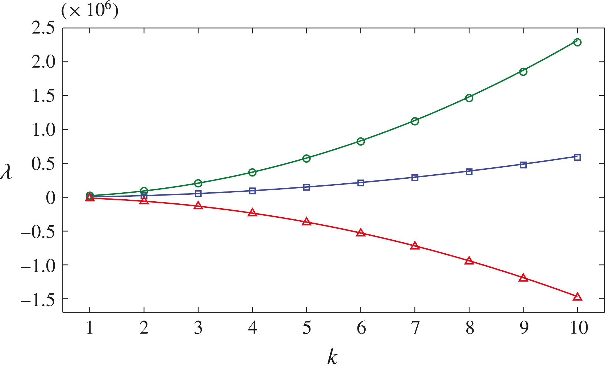
Figure 4 shows a comparison between the simulated growth rate for different values of the wavenumber parameterized by
 $k$
and that predicted theoretically using (2.35). Although the theoretical growth rate is an asymptotic result derived in the high-wavenumber limit, the numerical results lie very close to the quadratic curves predicted by the theory. Since the inertial number is fixed at a value of
 $I=5.3\times 10^{-5}$
in these simulations by having a constant strain rate across the domain, the values of
 $I_{0}^{-1}$
can be taken to be indicative of the deformation rate. The red line and the triangular symbols show an intermediate strain-rate case, with
 $I_{0}=1\times 10^{-4}$
, that lies in the well-posed region of parameter space and the perturbation decays for all wavenumbers
 $k$
. However, for both high and low strain rates indicated by the green circles and the blue squares, respectively, the growth rates are positive for all wavenumbers and the rate increases quadratically with increasing wavenumber. The numerical results therefore provide a finite-wavenumber confirmation of ill-posedness in the high-wavenumber limit.
A comparison of the numerical growth rate
 ${\it\lambda}$
(points) for perturbations of a fixed direction but differing wavenumber magnitudes
 $2{\rm\pi}k$
, with the theoretical growth rate predicted by the asymptotic formula (2.35) for large wavenumbers shown by the lines. The three symbols represent values of
 $I_{0}$
taken to be representative of the distinct stability regions with
 $I_{0}=1\times 10^{-6}$
(○) being a high strain-rate case,
 $I_{0}=1\times 10^{-4}$
(▵) being intermediate and
 $I_{0}=1$
(▫) representing a low strain rate.
The numerical scheme is also tested for a fixed wavenumber (
 $k=5$
) with variation in both
 $I_{0}$
and
 ${\rm\Delta}{\it\mu}$
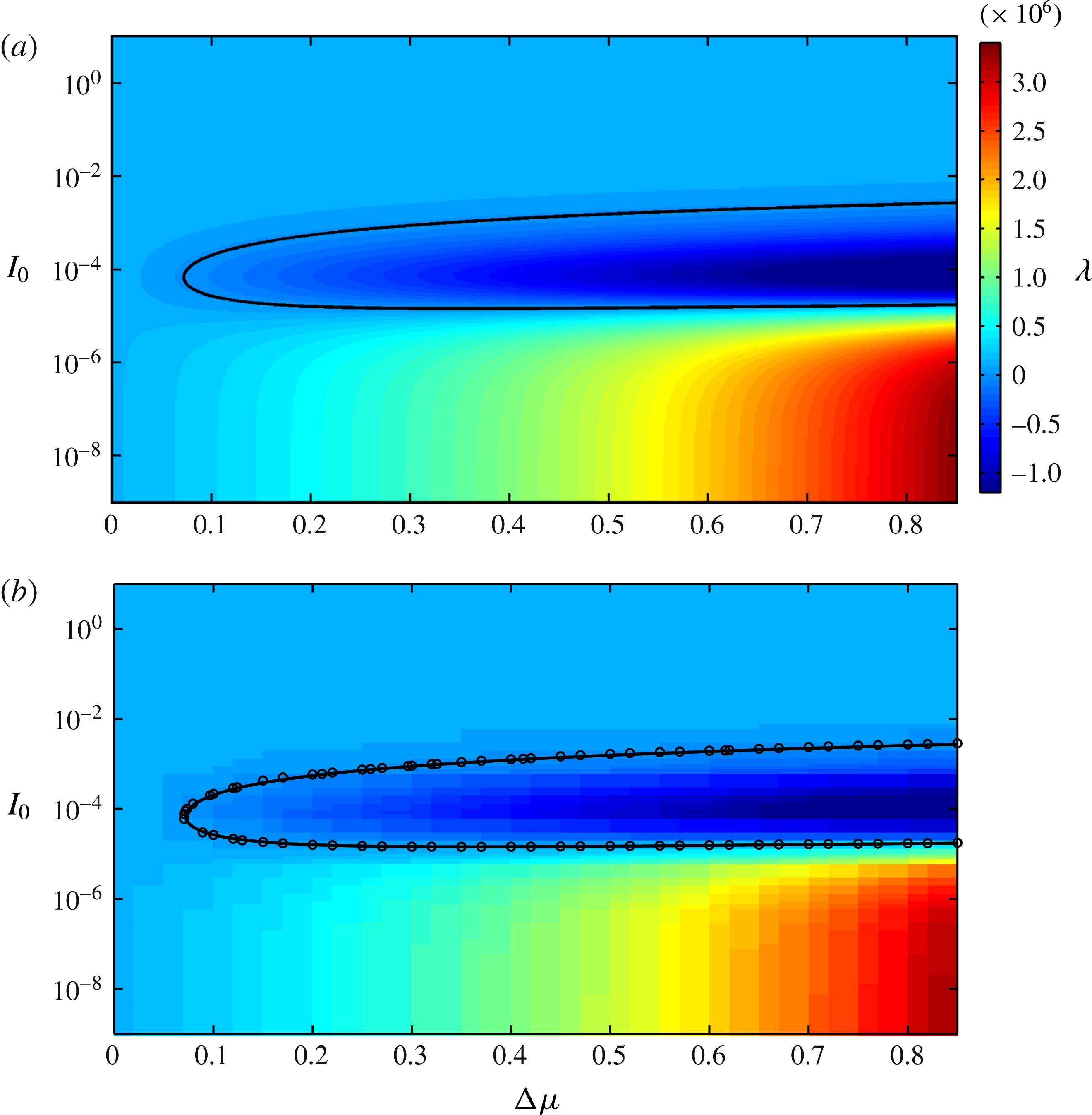
as shown in figure 5. Figure 5(a) shows the theoretical growth rate
 ${\it\lambda}$
predicted by (2.35) with fixed
 $I=5.3\times 10^{-5}$
, while figure 5(b) shows the numerically measured growth rate. The black neutral stability curve, shown in both plots, is equivalent to that shown in figure 2. The black circles in figure 5(b) show the numerically predicted neutral stability curve, which lies in very close agreement with the theory. This indicates that, provided
 ${\rm\Delta}{\it\mu}$
is sufficiently large, there are a wide range of intermediate values of
 $I_{0}$
where the growth is negative, perturbations decay and the equations are well-posed. Conversely when
 ${\rm\Delta}{\it\mu}$
is sufficiently small or when
 $I_{0}$
is large, or small, the growth rate is positive and perturbations will grow. At the fixed wavenumber
 $k=5$
the growth rates are finite, but as the wavenumber is increased the growth rate becomes ever stronger, which implies ill-posedness in the high-wavenumber limit.
A comparison of the theoretical (a) and numerical (b) growth rates for the system (3.5). Here, the solid black line is the theoretical neutral stability curve whereas the black circles are zero points interpolated from the numerical data set.
4. Application to unsteady Bagnold flow
It is also useful to demonstrate that our analysis of ill-posedness works for systems with non-constant base states in practical flow configurations. Consider the two-dimensional steady-uniform-depth Bagnold flow down a plane inclined at an angle
 ${\it\zeta}$
to the horizontal (e.g. GDR-MiDi 2004; Gray & Edwards Reference Gray and Edwards2014). The
 $x$
coordinate is assumed to point down the plane and the
 $z$
coordinate is the upwards pointing normal. Mass balance (2.3) is automatically satisfied if the normal velocity
 $w$
is equal to zero everywhere and the downslope velocity
 $u$
is a function of
 $z$
only. In this situation the normal momentum balance can be integrated, subject to the condition that the pressure is zero at the free surface at
 $z=h$
, to show that the scaled pressure is lithostatic, i.e.
 $$\begin{eqnarray}p_{{\it\zeta}}=g(h-z)\cos {\it\zeta},\end{eqnarray}$$
where
 $g$
is the constant of gravitational acceleration. Note that the factor
 ${\it\rho}{\it\phi}$
is missing in (4.1) because the pressure was scaled just after (2.10) to simplify the governing equations. The downslope momentum balance reduces to
 ${\it\mu}=\tan {\it\zeta}$
, so
 ${\it\mu}$
is equal to a constant on a slope of fixed inclination. It follows from (2.8) that at a given slope angle the inertial number is also equal to a constant
 $I_{{\it\zeta}}$
, where
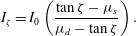 $$\begin{eqnarray}I_{{\it\zeta}}=I_{0}\left(\frac{\tan {\it\zeta}-{\it\mu}_{s}}{{\it\mu}_{d}-\tan {\it\zeta}}\right).\end{eqnarray}$$
Since the inertial number is constant, (2.11) becomes an ordinary differential equation for the Bagnold velocity profile, which can be solved subject to the no-slip condition at the base to show that
 $$\begin{eqnarray}u=\frac{2I_{{\it\zeta}}}{3d}\sqrt{{\it\phi}g\cos {\it\zeta}}\left(h^{3/2}-(h-z)^{3/2}\right).\end{eqnarray}$$
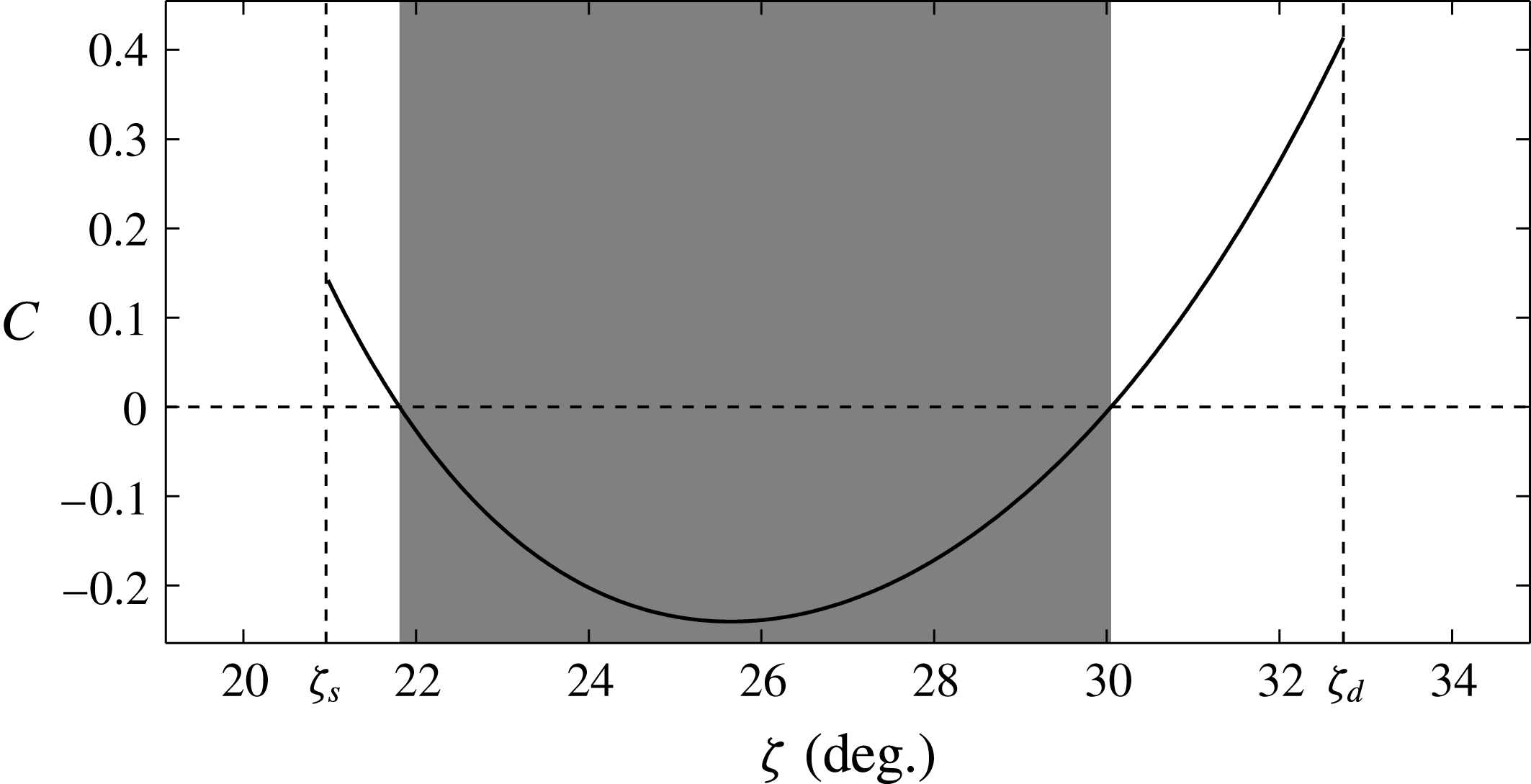
Figure 6 shows a plot of the values of the ill-posedness condition (2.43) for Bagnold flow using the material parameters in table 1 and
 $I_{0}=0.279$
. Note that
 ${\it\zeta}_{s}$
and
 ${\it\zeta}_{d}$
are the angles whose tangent is equal to
 ${\it\mu}_{s}$
and
 ${\it\mu}_{d}$
, respectively, i.e.
 ${\it\mu}_{s}=\tan {\it\zeta}_{s}$
and
 ${\it\mu}_{d}=\tan {\it\zeta}_{d}$
. These angles are the minimum and maximum angles for which steady-uniform flows develop. In the shaded area the function is negative and the equations are well-posed, whereas in the unshaded regions the function is positive and ill-posedness is anticipated. Note that our results are consistent with the linear stability analysis of Forterre (Reference Forterre2006), who also used the same parameters as in table 1 and
 $I_{0}=0.279$
. For an imposed forcing frequency, Forterre (Reference Forterre2006) experimentally measured the spatial growth rate of Kapiza or roll waves for a range of inclination angles and Froude numbers and was able to convincingly match the measured growth rates by performing a two-dimensional linear stability analysis with the
 ${\it\mu}(I)$
-rheology and Bagnold flow as a base state. For inclination angles in the range 24–29° he showed that there was a well-defined cutoff frequency above which higher frequencies decayed increasingly rapidly. All of these angles lie within the well-posed range, which is from approximately 22° to 30°, as shown in figure 6. For this range of angles the flow is linearly unstable for a finite range of wavenumbers or frequencies, but in the high-wavenumber or high-frequency limit the perturbations decay and the system is well-posed.
The value of the ill-posedness condition
 $C=4{\it\nu}^{2}-4{\it\nu}+{\it\mu}^{2}(1-{\it\nu}/2)^{2}$
(2.43) for the Bagnold flow solution with material parameters given in table 1 and with
 $I_{0}=0.279$
. Note that
 ${\it\mu}_{s}=\tan {\it\zeta}_{s}$
and
 ${\it\mu}_{d}=\tan {\it\zeta}_{d}$
. Here the range of well-posed angles is shaded grey.
The range of angles that are well-posed for the full
 ${\it\mu}(I)$
-rheology is smaller than the range for the depth-averaged
 ${\it\mu}(I)$
-rheology (Gray & Edwards Reference Gray and Edwards2014), which has negative viscosities and is hence ill-posed, for angles
 ${\it\zeta}\leqslant {\it\zeta}_{s}$
and
 ${\it\zeta}>{\it\zeta}_{d}$
outside the region where steady-uniform flows develop. It is therefore possible to push the depth-averaged
 ${\it\mu}(I)$
-rheology somewhat further than the full rheology. This has allowed the coarsening of roll waves and erosion–deposition waves to be calculated using the depth-averaged theory, without getting into issues of ill-posedness (Gray & Edwards Reference Gray and Edwards2014; Razis et al.
Reference Razis, Edwards, Gray and van der Weele2014; Edwards & Gray Reference Edwards and Gray2015).
Our analysis predicts that the
 ${\it\mu}(I)$
-rheology will be ill-posed for slow flows close to the minimum angle for steady-uniform flow and for fast flows close to the maximum angle for steady-uniform flow. As a validation of ill-posedness of the Bagnold flow in this regime, figures 7 and 8 show the results of a transient two-dimensional computation using the Gerris package, which has previously been used by Lagrée et al. (Reference Lagrée, Staron and Popinet2011) and Staron et al. (Reference Staron, Lagrée and Popinet2012) for granular column collapse and silos. The simulations are initialized with the Bagnold solution (4.1)–(4.3) and a no-slip boundary condition is applied at the base of the flow. In contrast to the computations performed in § 3 no perturbation is applied directly to the flow here. Instead, numerical noise is found to be sufficient to trigger the ill-posedness. To maintain a constant inertial number in the exact solution (4.1)–(4.3), the shear rate and the square root of the pressure both have to tend to zero at the same rate as the free surface is approached. This is difficult to achieve numerically in time-dependent and spatially dependent solutions. Gerris therefore takes the absolute value of the pressure to prevent complex inertial numbers from developing. In order to avoid this, computations are limited to a subset of the domain
 $z\in [0,s]=[0,0.01]~\text{m}$
by choosing a height
 $s<h$
at which the pressure
 $p_{{\it\zeta}}(s)=p_{s}$
is constant. This allows the Bagnold base state to be maintained without encountering singular or undefined limits. Note that a complementary shear stress is applied at
 $z=s$
, so that the classical Bagnold solution is maintained, and there is no free surface deformation, so roll waves are suppressed.
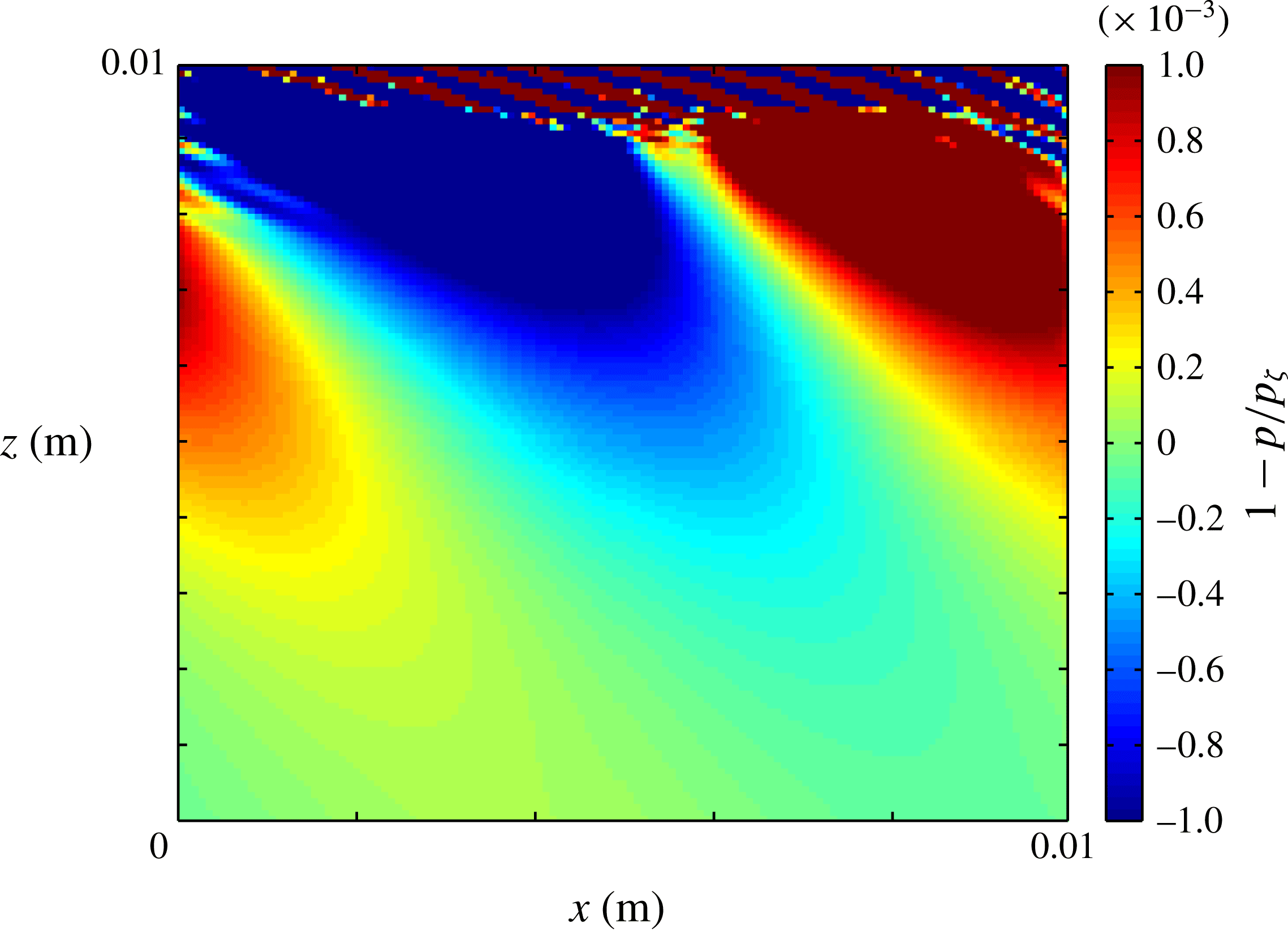
A snapshot at
 $t=0.06~\text{s}$
of the pressure
 $p$
relative to the lithostatic pressure
 $p_{{\it\zeta}}$
, given by (4.1), for the ill-posed angle
 ${\it\zeta}=32^{\circ }$
. The material parameters are given in table 1 and
 $I_{0}=0.279$
. An animation showing the complete time-dependent evolution of the solution is available in the online supplementary material. The simulation uses a Cartesian grid of
 $128\times 128$
cells with a time step of
 $1\times 10^{-5}~\text{s}$
and
 $p_{s}=1\times 10^{-3}$
. Note that for this flow the Froude number
 $\mathit{Fr}=(2/5)I_{{\it\zeta}}h\sqrt{{\it\phi}}/d\simeq 28.1$
.
A semi-log plot of the temporal behaviour of the error
 $E_{p}=\max (|1-p/p_{{\it\zeta}}|)$
between the hydrostatic and transient pressure for the Bagnold base state. The upper red points are computed for the ill-posed inclination angle
 ${\it\zeta}=32^{\circ }$
and the lower blue ones are for a well-posed angle of
 ${\it\zeta}=26^{\circ }$
.
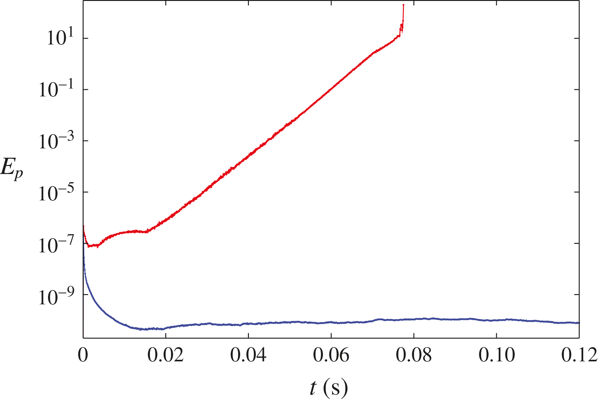
For angles in the well-posed (shaded) region of parameter space in figure 6, the simulations yield a pressure that is very close to the exact solution. A specific example of this is shown by the decay in the relative pressure error
 $E_{p}=\max (|1-p/p_{{\it\zeta}}|)$
in figure 8 for the case of
 ${\it\zeta}=26^{\circ }$
. However, for an angle of
 ${\it\zeta}=32^{\circ }$
, which lies in the ill-posed region of parameter space, small pressure perturbations develop (see figure 7) close to the free surface, which grow in size as shown in figure 8 and the supplementary movie available at http://dx.doi.org/10.1017/jfm.2015.412. This simulation therefore gives a specific example in which the fully nonlinear system with physically realistic boundary conditions breaks down due to ill-posedness, and further, demonstrates the importance of the condition (2.43) to systems with non-constant base states. It is interesting that numerical noise is sufficient to seed the ill-posedness, rather than having to impose a small perturbation. The perturbations are at the grid scale and grow rapidly in time, which indicates that the ill-posedness is a very strong effect that is not regularized at this resolution (here comparable to the grain size,
 $d$
). Figure 8 shows a semi-log plot of the relative pressure error
 $E_{p}=\max (|1-p/p_{{\it\zeta}}|)$
which implies catastrophic exponential growth at this resolution. It should be noted, however, that at lower resolutions numerical viscosity may be sufficient to suppress the ill-posedness.
It could be argued that the instability shown in figures 7 and 8 is related to the roll-wave instability (Forterre Reference Forterre2006; Gray & Edwards Reference Gray and Edwards2014; Razis et al.
Reference Razis, Edwards, Gray and van der Weele2014) since the flow is significantly above the critical Froude number
 $\mathit{Fr}_{c}\simeq 0.519$
for the full
 ${\it\mu}(I)$
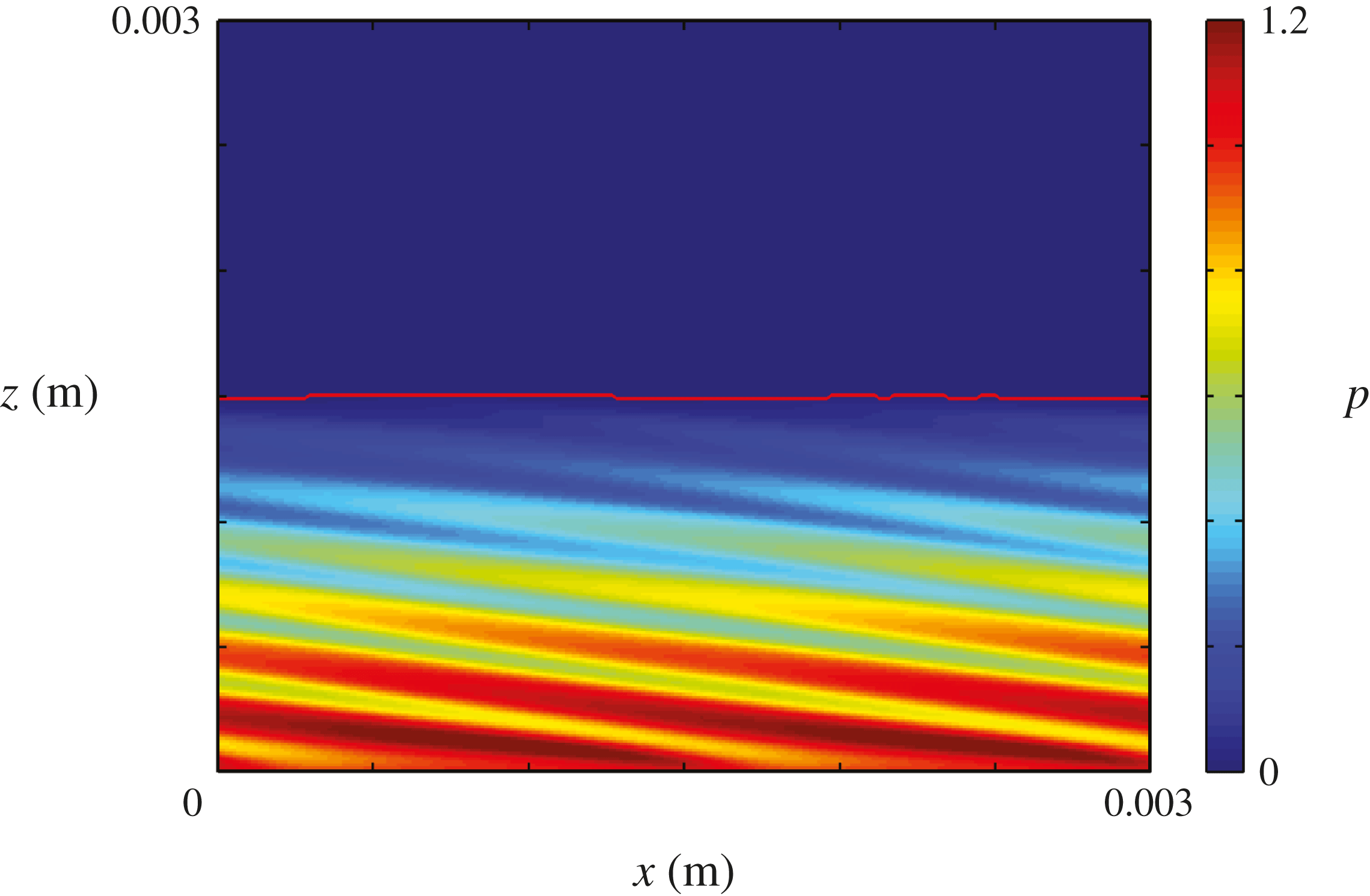
-rheology (Forterre Reference Forterre2006). To eliminate this possibility we have also conducted numerical simulations below the critical Froude number, which show the same behaviour. In addition, we have used Lagrée et al.’s (Reference Lagrée, Staron and Popinet2011) two-fluid implementation to allow the free surface to deform. Figure 9 shows a snapshot of the non-dimensional pressure field, just before the simulation fails, in which the same oblique pressure perturbations are seen to develop before any significant deformation of the free surface. In these simulations the granular material initially occupies the region
 $0<z<1.5~\text{mm}$
, the passive low-viscosity fluid occupies the region
 $1.5<z<3~\text{mm}$
and a slightly modified Bagnold solution (that accounts for the pressure and the shear stress applied by the fluid above) is used as an initial condition. Since this configuration is stable to roll waves, this problem provides a simple example of an instability whose most likely cause is the ill-posedness of the equations in the high-wavenumber limit. Note that although both the problems illustrated in figures 7 and 9 have a strictly positive initial pressure distribution the oblique pressure perturbations are sufficient to produce zero pressure at some point in the domain, which causes the code to fail.
A snapshot at
 $t=0.04~\text{s}$
of the non-dimensional pressure
 $p$
(i.e. scaled by the basal lithostatic pressure) for a simulation with a deformable free surface indicated by the solid red line and at the ill-posed angle
 ${\it\zeta}=32^{\circ }$
. The granular material parameters are given in table 1 and
 $I_{0}=0.279$
. Lagrée et al.’s (Reference Lagrée, Staron and Popinet2011) two-fluid implementation is used with a passive low-viscosity fluid of density ratio
 ${\it\rho}_{f}/({\it\rho}{\it\phi})=1\times 10^{-3}$
. The simulation uses a Cartesian grid of
 $256\times 256$
cells with a time step of
 $1\times 10^{-5}~\text{s}$
. Note that for this flow the Froude number
 $\mathit{Fr}=(2/5)I_{{\it\zeta}}h\sqrt{{\it\phi}}/d\simeq 0.42$
.
5. Conclusions and discussion
This paper shows that in two dimensions the
 ${\it\mu}(I)$
-rheology (GDR-MiDi 2004; Jop et al.
Reference Jop, Forterre and Pouliquen2005, Reference Jop, Forterre and Pouliquen2006) is well-posed for a large intermediate range of inertial numbers, provided
 ${\rm\Delta}{\it\mu}$
is sufficiently large, but that for both high and low inertial numbers the equations are ill-posed. This is a significant improvement over the classical Coulomb rheology with a von Mises yield criterion, which is always ill-posed in two dimensions (Schaeffer Reference Schaeffer1987). Our analysis yields a simple inequality (2.43) to determine whether a problem is locally ill-posed or not. Knowing that a problem is ill-posed is very important, because it is telling you that there is some important missing physics (Fowler Reference Fowler1997). If the problem is ill-posed, small perturbations grow at an unbounded rate in the high-wavenumber limit, i.e. a catastrophic short-wavelength (Hadamard) instability (Joseph & Saut Reference Joseph and Saut1990). As a result, as the grid resolution of a numerical scheme is refined, higher wavenumbers will be resolved and the instability will grow progressively stronger, leading to grid-dependent results. The two-dimensional time-dependent numerical simulations of steady-uniform Bagnold flow down an inclined plane using Gerris (Lagrée et al.
Reference Lagrée, Staron and Popinet2011; Staron et al.
Reference Staron, Lagrée and Popinet2012), shown in figures 7 and 9 (and the supplementary movie), indicate that strong pressure and velocity fluctuations develop that eventually break the computation for slopes outside the well-posed range of angles that are shown in figure 6.
Note that a simple method of suppressing the ill-posedness is to solve a steady-state problem in which the time derivative is eliminated. This was done by Jop et al. (Reference Jop, Forterre and Pouliquen2005) in order to calculate the downslope velocity as a function of cross-slope position and depth. This is not always a practicable approach, but it necessarily leads to a well-posed two-dimensional elliptic problem, which may provide a useful solution in certain instances. When time dependence and an extra spatial dimension are reintroduced we suspect that the
 ${\it\mu}(I)$
-rheology will still develop zones of ill-posedness. It is noteworthy that Schaeffer (Reference Schaeffer1987) showed that the Coulomb rheology with a von Mises yield criterion was sometimes well-posed in three dimensions. It follows that the
 ${\it\mu}(I)$
-rheology is likely to be somewhat better posed in three dimensions, but zones of ill-posedness are still expected, although we have not proved this.
The fact that the
 ${\it\mu}(I)$
-rheology is well-posed in the dense inertial regime and can be used to model complex flows in chutes (Forterre Reference Forterre2006; Jop et al.
Reference Jop, Forterre and Pouliquen2006; Gray & Edwards Reference Gray and Edwards2014; Edwards & Gray Reference Edwards and Gray2015) provides strong evidence that it is a good constitutive law for liquid-like granular flows. The challenge for the future is to include new physics, so that the rheology can transition seamlessly between the quasi-static, dense inertial and collisional flow regimes. Most problems of practical interest will span the complete range of the inertial number
 $I$
, and even the simplest of flows, such as a sand clock, the formation of heaps or the rotation of grains in a drum, will span all three regimes. This is therefore a major challenge. There is, however, some hope as Lagrée et al. (Reference Lagrée, Staron and Popinet2011) and Staron et al. (Reference Staron, Lagrée and Popinet2012) have had some success at modelling granular column collapse and flow in silos using the
 ${\it\mu}(I)$
-rheology, even though there are significant regions within their domain that lie outside the well-posed region of parameter space. Their success may in part be due to the ad hoc regularizations that they have introduced to eliminate the singularity in the viscosity at low strain rate (2.10) and the finite pressure imposed at the free surface, which reduces the range of the inertial parameter. It may also be possible that, by using a coarse mesh (large grid spacing), such simulations avoid the effects of the ill-posedness by suppressing the faster growing, high-wavenumber modes.
One might then naively ask why not always solve the equations numerically at a finite resolution that is representative of the grain scale? This would provide a means of truncating the allowable range of wavenumbers and hence avoid the singularity in an ill-posed problem for the high-wavenumber limit. While this approach may be appealing, it is ultimately unsatisfactory. This is because this ad hoc form of regularization relies on the numerical viscosity inherent in the specific numerical scheme, rather than a rational and physically motivated regularization of the equations. Above a specific resolution the numerical viscosity alone may not even be sufficient to prevent the code from breaking, as evidenced by the simulations in § 4. Even if the algorithm does converge, different numerical methods may produce different results, even though the same continuum equations are claimed to be being solved. This would be a retrogressive step that would lead to great confusion. Besides, understanding what the right physics is, is an important scientific journey in itself.
Based on the discrete particle simulations of da Cruz et al. (Reference da Cruz, Emam, Prochnow, Roux and Chevoir2005), Pouliquen et al. (Reference Pouliquen, Cassar, Jop, Forterre and Nicolas2006) extended the
 ${\it\mu}(I)$
-rheology to include a dependence of the solids volume fraction on the inertial number, i.e.
 ${\it\phi}={\it\phi}_{max}-({\it\phi}_{max}-{\it\phi}_{min})I$
, where typically
 ${\it\phi}_{max}=0.6$
and
 ${\it\phi}_{min}=0.5$
. This is a slightly odd relation, because the solids volume fraction will become negative for
 $I>{\it\phi}_{max}/({\it\phi}_{max}-{\it\phi}_{min})$
, which is clearly incorrect for high inertial numbers. While this is easy to fix, it is not clear whether the inclusion of an additional
 ${\it\phi}(I)$
dependence will be sufficient to prevent ill-posedness. Pitman & Schaeffer (Reference Pitman and Schaeffer1987) and Schaeffer & Pitman (Reference Schaeffer and Pitman1988) showed that in three dimensions Critical State Soil Mechanics is well-posed provided that each of the principal strain rates does not tend to zero anywhere in the flow. It follows that even a small amount of dilation/compaction can have an important regularizing influence. An important extension of this work will therefore be to include the
 ${\it\phi}(I)$
dependence. Rather intriguingly, the rheology of dense suspensions is closely related to that of granular flow, with two functions
 ${\it\mu}={\it\mu}(I_{{\it\nu}})$
and
 ${\it\phi}={\it\phi}(I_{{\it\nu}})$
that depend on a dimensionless viscous number
 $I_{{\it\nu}}$
instead of
 $I$
(Boyer, Guazzelli & Pouliquen Reference Boyer, Guazzelli and Pouliquen2011a
; Boyer, Pouliquen & Guazzelli Reference Boyer, Pouliquen and Guazzelli2011b
; Couturier et al.
Reference Couturier, Boyer, Pouliquen and Guazzelli2011). Such an extension of our analysis may therefore have important implications for dense suspensions as well.
At very high inertial number (
 $I>10^{-1}$
) the flow becomes so dilute that it turns into a granular gas. Models in this area are very well developed (see e.g. Jenkins & Savage Reference Jenkins and Savage1983; Goldhirsch Reference Goldhirsch2003) and Jenkins (Reference Jenkins2006) has made progress in analysing the transition from dilute to dense regimes using a phenomenological modification of the theory. Such a transition may need to be incorporated close to the free surface to prevent singularities and undefined values from arising with the
 ${\it\mu}(I)$
-rheology. The transition to quasi-static flows for
 $I<10^{-3}$
is also problematic. Here the flow becomes rate-independent and deformation may become localized in shear bands (Vardoulakis, Goldscheider & Gudehus Reference Vardoulakis, Goldscheider and Gudehus1978) whose width is dependent on the grain size. The soil mechanics community have developed many models for shear banding, including higher gradient theories (Vardoulakis & Aifantis Reference Vardoulakis and Aifantis1991), Cosserat theories (Tejchman & Gudehus Reference Tejchman and Gudehus2001) and Hypoplastic models (Wu et al.
Reference Wu, Bauer and Kolymbas1996). Kamrin (Reference Kamrin2010) combined the
 ${\it\mu}(I)$
-rheology with Jiang & Liu’s (Reference Jiang and Liu2003) model for granular elasticity and was able to compute steady-state solutions for rough-walled chute flow and an annular Couette cell as well as time-dependent solutions for a flat-bottomed silo. More recently it has been recognized that force chains (Howell et al.
Reference Howell, Behringer and Veje1999) provide a mechanism of rapidly transmitting stress fluctuations through the material in the quasi-static regime. One example of this apparently non-local behaviour is the ability of a finite thickness of granular material to remain stationary on an inclined plane between the angles
 ${\it\zeta}_{1}$
and
 ${\it\zeta}_{2}$
, which is not predicted by the local nature of the
 ${\it\mu}(I)$
-rheology. Pouliquen & Forterre (Reference Pouliquen and Forterre2009) formulated a non-local model based on the idea of a self-activated process. This produced an integral equation linking the pressure, the shear stress and the shear rate, which was able to predict a minimum thickness for flow to occur at a given inclination angle, i.e.
 $h_{stop}({\it\zeta})$
. However, the experimentally observed collapse of
 $h/h_{stop}$
as a function of Froude number was no longer reproduced. An alternative non-local approach uses an order parameter called the ‘fluidity’ to diffuse fluctuations away from the point where they are generated (Bocquet, Colin & Ajdari Reference Bocquet, Colin and Ajdari2009; Kamrin & Koval Reference Kamrin and Koval2012; Bouzid et al.
Reference Bouzid, Trulsson, Claudin, Clément and Andreotti2013) and hence allow material to flow even though it is below the yield stress. This promising approach has been used by Henann & Kamrin (Reference Henann and Kamrin2013) to accurately compute the two-dimensional steady-state flow in a split-bottom cell. It remains to be seen whether these theories are able to reproduce the experimental observations of Toiya et al. (Reference Toiya, Stambaugh and Losert2004), where flow reversal destroyed the anisotropy of the contact fabric and induced flow far from the shear surface, where one might anticipate that microstructural theories (e.g. Sun & Sundaresan Reference Sun and Sundaresan2011) will be required. In all of these approaches it is unclear whether the additional physics is sufficient to regularize the models, but there is certainly considerable hope that continuum theories will be able to compute fully time-dependent flows in practical configurations, such as heaps, drums and silos, in the foreseeable future.
Acknowledgements
This research was supported by NERC grants NE/E003206/1 and NE/K003011/1 as well as EPSRC grants EP/I019189/1, EP/K00428X/1 and EP/M022447/1. Bohorquez acknowledges the financial support by the Caja Rural Provincial de Jaén and the University of Jaén (project no. UJA2014/07/04). N. Gray acknowledges support from the program on ‘Fluid-Mediated Particle Transport in Geophysical Flows’ at the Kavli Institute for Theoretical Physics, Santa Barbara, USA.
Supplementary movies
Supplementary movies are available at http://dx.doi.org/10.1017/jfm.2015.412.


 Open access

