Simplified estimation of forage degradability in the rumen assuming zero-order degradation kinetics

M. S. DHANOA; S. LÓPEZ; R. SANDERSON; J. FRANCE

doi:10.1017/S0021859608008241

Simplified estimation of forage degradability in the rumen assuming zero-order degradation kinetics

Published online by Cambridge University Press: 08 December 2008

R. SANDERSON and

M. S. DHANOA: Affiliation:
Institute of Grassland and Environmental Research (IGER)†, Plas Gogerddan, Aberystwyth, Ceredigion, SY23 3EB, UK
S. LÓPEZ*: Affiliation:
Instituto de Ganadería de Montaña (IGM), Universidad de León – Consejo Superior de Investigaciones Científicas (CSIC), Departamento de Producción Animal, Universidad de León, E-24071 León, Spain
R. SANDERSON: Affiliation:
Institute of Grassland and Environmental Research (IGER)†, Plas Gogerddan, Aberystwyth, Ceredigion, SY23 3EB, UK
J. FRANCE: Affiliation:
Centre for Nutrition Modelling, Department of Animal and Poultry Science, University of Guelph, Guelph, ON, N1G 2W1, Canada
*: *To whom all correspondence should be addressed. Email: s.lopez@unileon.es

Article contents

Summary
INTRODUCTION
MATERIALS AND METHODS
RESULTS
DISCUSSION
CONCLUSIONS
Footnotes
References

Rights & Permissions

Summary

In the present paper, a simplified procedure using few in situ data points is derived and then evaluated (using a large database) against reference values estimated with the standard nylon bag first-order kinetics model. The procedure proposed involved a two-stage mathematical process, with a statistical prediction of some degradation parameters (such as lag time) and then a kinetic model derived by assuming degradation follows zero-order kinetics to determine effective degradability in the rumen (E). In addition to the estimation of washout fraction and discrete lag, which is common to both procedures, the simplified procedure requires measurement of dry matter losses at one incubation time point only. Thus, interference of the animal rumen will be much reduced, which will lead to increased capacity for feed evaluation. Calibration of the zero-order model against the first-order model showed that suitable estimates of E can be obtained with disappearance at 24, 48 or 72 h as the single incubation end time point. The strength of the calibration is such that an end incubation time point as low as 24 h may be sufficient, which may reduce substantially the total incubation time required and thus the impact on the experimental animal. Relevant regression equations to predict reference values of parameters such as lag time or E are also developed and validated.

Information

Type: Modelling Animal Systems Paper
Information: The Journal of Agricultural Science , Volume 147 , Issue 3 , June 2009, pp. 225 - 240
DOI: https://doi.org/10.1017/S0021859608008241 [Opens in a new window]
Copyright: Copyright © 2008 Cambridge University Press

INTRODUCTION

Artificial synthetic fibre bag in situ procedures, which have evolved since the earlier part of the 20th century, are a standard means of estimating the extent of degradation of ruminant feeds (Ørskov & McDonald Reference Ørskov and McDonald1979; López Reference López, Dijkstra, Forbes and France2005). Feed samples are enclosed in the bag and then suspended in the rumen, hence removing the effect of passage or outflow but allowing the degradation of the substrate within the bag by ruminal microbes. Pore size should permit free flow of microbes in and out of the bag, with the risk that undegraded small particulate matter may escape from the bag (López Reference López, Dijkstra, Forbes and France2005). Thus, it is necessary to make the assumption that substrate disappearance from the bag represents substrate degradation by ruminal microbes and that particulate matter escaping from the bag is instantly and completely degraded (Dhanoa et al. Reference Dhanoa, France, López, Dijkstra, Lister, Davies and Bannik1999a). Even if this is true for the truly soluble fraction, it is unlikely to be true for the mechanical loss of undegraded particulate matter. Furthermore, it is inevitable that the soluble fraction, commonly referred to as the wash fraction, tends to be overestimated and various correction or adjustment procedures have been proposed to mitigate the effects of estimate bias of the wash fraction (Dhanoa et al. Reference Dhanoa, France, López, Dijkstra, Lister, Davies and Bannik1999a).

In addition, the in situ procedure requires greater amounts of sample than in vitro methods, may be laborious and time consuming and may have a heavy impact on the host animal with regard to the number of bags per run and number of incubation sampling times needed to obtain sufficient data so that the chosen kinetic model (e.g. Ørskov & McDonald Reference Ørskov and McDonald1979; McDonald Reference McDonald1981; Dhanoa Reference Dhanoa1988; López Reference López, Dijkstra, Forbes and France2005; Mertens Reference Mertens, Dijkstra, Forbes and France2005) may be fitted. These issues may hamper widespread use of the technique as a routine method of feed evaluation, because the above requirements may mean that only a few feeds can be handled at a time and repeated runs are necessary to overcome low capacity problems. This requires the use of more animals and/or repeated use of some animals, which is contrary to the principle of least invasive experimentation. Use of more animals also has added difficulties, such as confounding of feed effects and animal effects. A statistical design of the study can help but the overall workload on the animals may increase. Despite the widespread use and detailed application of the nylon bag procedure, several alternatives have been proposed to overcome all difficulties associated with the technique without any loss in accuracy of the measurements.

Rate and extent of degradation of feeds in the rumen are usually estimated from in situ disappearance curves, by fitting a non-linear equation to obtain estimates of several degradation parameters (France et al. Reference France, Thornley, López, Siddons, Dhanoa, Van Soest and Gill1990; López Reference López, Dijkstra, Forbes and France2005; Mertens Reference Mertens, Dijkstra, Forbes and France2005). This common approach requires that disappearance at several incubation times be recorded. Thus, a simplified procedure with a reduced number of incubation times is worth considering and some approaches have been reported in the literature (Broderick Reference Broderick and Fahey1994; Olaisen et al. Reference Olaisen, Mejdell, Volden and Nesse2003). However, this alternative will need to be calibrated and validated against the full bag procedure as normally used, providing enough information from a large database of in situ data is available. The objective of the present study, therefore, is to derive and evaluate a simplified procedure, using few incubation data points and based on the assumption that ruminal degradation is a zero-order kinetic process, in relation to the currently used in situ procedure.

MATERIALS AND METHODS

General scheme

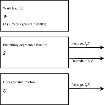
The main components of a specific feed entering the rumen are assumed to be: (1) a soluble fraction W (g) which is instantly and completely degraded, (2) a potentially degradable fraction S (g) and (3) a completely undegradable fraction U (g). Only S and U are of dynamic interest in estimating the rate and extent of degradation as W is assumed to be degraded instantly. A discrete lag L (h) will be assumed to occur before any degradation commences. The degradation and passage kinetics of S and U are shown in Fig. 1, where k _p (per hour) is the fractional or relative rate of passage from the rumen. The value of passage rate k _p is assumed known, as this parameter can be estimated using digesta flow markers by either ruminal or faecal sampling.

Fig. 1.

Feed fractions showing their degradation and passage kinetics in the rumen.

Mathematical formulation

When feed is incubated in situ in artificial fibre (polyester, nylon or dacron) bags suspended in the rumen or in vitro in a flask containing rumen fluid, the rate of passage is zero. Pool dynamics as shown in Fig. 1 become

(1a)

$\hfill{\rm d}S\sol {\rm d}t \equals 0\comma \quad0\les t \lt L\hfill$

(1b)

$\hfill \hskip22pt\equals \minus F\comma \quad t\ges L\hfill$

and

(2)

${\rm d}U\sol {\rm d}t \equals 0\comma \quad t\ges 0$

where F is the degradation rate (g/h).

On integration, Eqns (1a) and (2) give

$\openup3\matrix{ {S \equals S_{\setnum{0}} \comma } \hfill \tab {0\les t \lt L} \hfill \cr {U \equals U_{\setnum{0}} \comma } \hfill \tab {t\ges 0} \hfill \cr}$

respectively, where S ₀ is potentially degradable substrate at the start of the incubation, and U ₀ is the completely undegradable fraction. From Eqn (1b) the amount of potentially degradable substrate (S; g) remaining in the bag or the flask at any incubation time t (t>L) can be calculated as

$S \equals S{}_{\setnum{0}} \minus \int_{L}^{t} {F\,{\rm d}t} \comma \quad t\ges L$

and the cumulative disappearance of substrate (D; g) to time t (t>L) becomes

$D\, \equals \,W \plus \int_{L}^{t} {F{\rm d}t} \comma \quad t\ges L$

The above equations for degradation in the rumen, when feed particles are subject to losses due to passage from the rumen, become

(3a)

$\hfill \hskip14{\rm d}S\sol {\rm d}t \equals \minus k_{\rm p} S\comma \quad 0\les t \lt L\hfill$

(3b)

$\hfill \hskip42pt\equals \minus F \minus k_{\rm p} S\comma \quad t\ges L\hfill$

and

(4)

${\rm d}U\sol {\rm d}t \equals \minus k_{\rm p} U\comma \quad t\ges 0$

On integrating Eqns (3a), (3b) and (4), the following are obtained:

$\hfill \hskip-28pt S\, \equals \,S{}_{\setnum{0}}\exp \lpar \minus k_{\rm p} t\rpar \comma \quad 0\les t \lt L\hfill$

$\hfill S \equals \bigg(S_{\setnum{0}} \minus \int_{L}^{t} {F{\rm e}^{k_{{\rm p}} t} {\rm d}t\bigg) } {\rm e}^{ \minus k_{{\rm p}} t} \comma \quad t\ges L\hfill$

$\hfill\hskip-45pt U\, \equals \,U{}_{\setnum{0}}\exp \lpar \minus k_{\rm p} t\rpar \comma \quad t\ges 0\hfill$

Extent of degradation or effective degradability (E) in the rumen proper is then

$E\, \equals \,W \plus \int_{L}^{\infty } {F\ {\rm d}t}$

Applying the concepts of chemical kinetics to the process of substrate degradation in the rumen, the degradation rate is linked to the amount of substrate remaining in the rumen (i.e. F=f(S)). This relationship has been represented mathematically by the rate equation or rate law:

$F\, \equals \,\mu \,S^{n}$

In this equation, μ is the degradation rate coefficient or rate constant, although it is not necessarily a constant, as it may include the effect of any factor that affects degradation rate (López et al. Reference López, France, Dhanoa, Mould and Dijkstra1999; France et al. Reference France, Dijkstra, Dhanoa, López and Bannink2000), except for S, which is explicitly taken into account. The exponent n is called reaction order and depends on the mechanism assumed to be responsible for the substrate degradation in the rumen. In the particular case of first-order kinetics, n=1, so that the rate of degradation assumes the mathematical form

${{{\rm d}S} \over {{\rm d}t}}\,\, \equals F\, \equals \,\mu \,S\comma \quad t\ges L$

where μ (per hour) is the specific or fractional rate of degradation. In the simplest first-order kinetics model, μ is assumed invariant, viz. μ=k _d, where k _d (per hour) is a constant. This case is the degradation model of Ørskov & McDonald (Reference Ørskov and McDonald1979) and McDonald (Reference McDonald1981). Eqn (1b) for describing the potentially degradable fraction of the feed component under incubation now yields the following expression for S:

$S\, \equals \,S_{\setnum{0}} {\rm e}^{ \minus k_{{\rm d}} \lpar t \minus L\rpar } \comma \quad t\ges L$

and the cumulative disappearance of substrate from the bag or flask becomes

(5)

$D\, \equals \,W \plus \,S{}_{\setnum{0}}\lpar 1 \minus {\rm e}^{ \minus k_{{\rm d}} \lpar t \minus L\rpar } \rpar \comma \quad t\ges L$

Fitting Eqn (5) to serial disappearance data using non-linear regression allows direct estimation of W, S ₀, k _d and L, as described by Dhanoa (Reference Dhanoa1988), and using these estimates, in conjunction with an estimate of passage rate k _p, permits calculation of the effective degradability in the rumen (E) by applying the equation

$E\, \equals \,W \plus {{k_{\rm d} \,} \over {k_{\rm d} \plus k_{\rm p} }}S{}_{\setnum{0}}\,{\rm e}^{ \minus k_{{\rm p}} L} \comma \quad t\ges L$

The above approach is the standard method for estimating rate and extent of degradation in the rumen.

Zero-order degradation

The degradation rate under this option has the mathematical form

(6)

${{{\rm d}S} \over {{\rm d}t}} \equals \minus F \equals \minus \mu S^{\setnum{0}} \equals \minus \mu \comma \quad t\ges L$

where μ (g/h) is now the actual degradation rate. If μ is invariant with time, then F is constant and Eqn (6) becomes

$\openup3\matrix{ {F \equals K\comma } \tab { \tab L\les t\les T} \cr {\hskip3\equals 0\comma } \tab {{\rm otherwise}} \cr}$

where K (g/h) is the constant degradation rate, and T (h) is the time at which all S ₀ is degraded and disappearance reaches its asymptotic value. With both equations, F is described as a zero-order process. Solving Eqn (1b), the potentially degradable feed fraction under incubation takes the following linear form:

(7a)

$S \equals S_{\setnum{0}} \minus K\lpar t \minus L\rpar \comma \quad L\les t\les \lpar L \plus S_{\setnum{0}} \sol K\rpar$

(7b)

$\hskip-60pt \equals 0\comma \quad t \gt \lpar L \plus S_{\setnum{0}} \sol K\rpar$

In Eqns (7a, b), T=L+S ₀/K. The instantaneous fractional degradation rate, a variable k _d (per hour), is given by

$k_{\rm d} \equals {K \over S}.$

The average fractional degradation rate over the interval (t ₁, t ₂), which lies inside (L, L+S ₀/K), is

$\eqalign{{k}_{\rm d} \tab \equals{1 \over {t_{\setnum{2}} \minus t_{\setnum{1}} }}\int_{t_{\setnum{1}} }^{t_{\setnum{2}} } {{K \over S}{\rm d}t} \cr\tab \equals{1 \over {t_{\setnum{2}} \minus t_{\setnum{1}} }}\int_{S_{\setnum{1}} }^{S_{\setnum{2}} } {{K \over S}\left( { \minus {{{\rm d}S} \over K}} \right)} \equals {1 \over {t_{\setnum{2}} \minus t_{\setnum{1}} }}\int_{S_{\setnum{2}} }^{S_{\setnum{1}} } {{{{\rm d}S} \over S}}$

${k}_{\rm d} \equals {{\ln S_{\setnum{1}} \minus \ln S_{\setnum{2}} } \over {t_{\setnum{2}} \minus t_{\setnum{1}} }}$

The cumulative degradation, from the bag or flask, on integration gives a piecewise segmented model with three straight lines as follows:

(8a)

$\hskip-96pt D \equals 0\comma \quad 0\les t \lt L$

(8b)

$\equals W \plus K\lpar t \minus L\rpar \comma \quad L\les t\les \lpar L \plus S_{\setnum{0}} \sol K\rpar$

(8c)

$\hskip-41pt \equals W \plus S_{\setnum{0}} \comma \quad t \gt \lpar L \plus S_{\setnum{0}} \sol K\rpar$

For a feed component placed in the rumen itself, where it is also subject to passage:

$\hfill\hskip2pt{{{\rm d}S} \over {{\rm d}t}} \equals \minus k_{p} S\comma \quad 0\les t \lt L\hfill$

$\hfill\hskip16pt\equals \minus K \minus k_{p} S\comma \quad t\ges L\hfill$

and integration of these equations gives

$\openup4\matrix{ {\hskip-6pt S \equals S_{\setnum{0}} {\rm e}^{ \minus k_{{\rm p}} t} \comma }\quad{0\les t \lt L} \hfill \cr \hfill{ \equals \left( {S_{\setnum{0}} \plus \displaystyle{K \over {k_{\rm p} }}{\rm e}^{k_{{\rm p}} L} } \right){\rm e}^{ \minus k_{{\rm p}} t} \minus \displaystyle{K \over {k_{\rm p} }}\comma } \hfill \tab {L\les t\les \tau } \hfill \cr \hfill{\hskip-78pt \equals 0\comma }\quad {t \gt \tau } \hfill \cr}$

where time τ (h) is given by $\tau \equals \ln \left( {{\textstyle{{k_{\rm p} S_{\setnum{0}} } \over K}} \plus {\rm e}^{k_{{\rm p}} L} } \right)\sol k_{\rm p}.$

The effective degradability (E) for the simple zero-order case becomes

$E\, \equals \,\,W \plus K\int_{L}^{\tau } {dt}$

giving

(9)

$E\, \equals \,\,W \plus {K \over {k_{\rm p} }}\ln \left( {{{k_{\rm p} S_{\setnum{0}} } \over K} \plus {\rm e}^{k_{{\rm p}} L} } \right) \minus KL$

Simplified procedure

Using serial cumulative disappearance data and non-linear regression, the estimates of parameters W, S ₀, K and L can be obtained from the zero-order kinetic model. This approach has been used before (López et al. Reference López, France, Dhanoa, Mould and Dijkstra1999), but requires a number of data points (i.e. disappearance values at different incubation times). Strictly speaking, at least two data points would be required for each segment (straight line) of the model.

Based on the mathematical formulation for zero-order kinetics, a novel approach to estimate effective degradability of feeds in the rumen is proposed. The approach requires few (one to three) data points. To develop this approach, a number of alternatives will be examined.

From Eqn (9), the parameters required for the determination of E are W, S ₀, L and K. Experimentally measured values of W and S ₀ are suitable for the purpose. W can be assumed to be the disappearance of matter obtained when bags containing a sample of feed are washed without incubation in the rumen. Washing should follow the same procedure used for all the bags incubated in the rumen and the wash value measured will include both the fraction of feed that is dissolved in water (soluble fraction) and the particulate matter that is mechanically lost from the bag.

The entity S ₀ can be calculated from disappearance of substrate after incubation in the rumen for a long time (D_∞). Assuming that D_∞ equals asymptotic substrate disappearance (i.e. W+S ₀), then S ₀=D_∞−W. This assumption requires that incubation time is long enough. In the simplified procedure, S ₀ was estimated using substrate disappearance recorded after 24, 48, 72 or 96 h of incubation, from which washout W was removed (i.e. S ₀=D−W).

The discrete lag time L cannot be measured experimentally and can be estimated only when a model is fitted to serial cumulative disappearance data. Estimates of L are highly dependent on the available disappearance data (for precise estimation, a large number of data points in the initial part of the curve at short incubation times is required) and on the model used to fit the curves, so that lag estimates using either the exponential (Eqn 5) or the segmented (Eqns 8a–c) model may be considerably different (López et al. Reference López, France, Dhanoa, Mould and Dijkstra1999). As a consequence, some authors have suggested that a discrete lag is a mathematical artefact derived from fitting non-linear models (López Reference López, Dijkstra, Forbes and France2005; Mertens Reference Mertens, Dijkstra, Forbes and France2005). In the present work, to simplify the model, it was assumed that L=0, thus $E \equals W \plus {\textstyle{K \over {k_{\rm p} }}}\ln \left( {{\textstyle{{k_{\rm p} S_{\setnum{0}} } \over K}} \plus 1} \right).$ Nevertheless, to test the influence of inclusion of a lag estimate, the simplified procedure was also applied using the lag estimates obtained previously by fitting the exponential (first-order) model.

The parameter K is the slope of the straight line representing the phase between the lag time and the time at which asymptotic disappearance is reached, i.e.

$K \equals {{D \minus W} \over {t \minus L}}\comma \quad L\les t\les \lpar L \plus S_{\setnum{0}} \sol K\rpar$

If L=0, then

$K \equals {{D \minus W} \over t}\comma \quad 0 \lt t\les \lpar S_{\setnum{0}} \sol K\rpar$

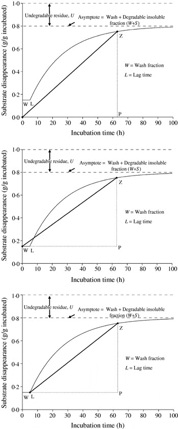
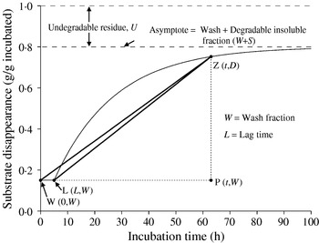
In the simplified method, several alternatives will be evaluated to estimate K, from different combinations of disappearance values at early and late incubation times. Thus, for the final point, disappearance values at 24 h (D ₂₄), 48 h (D ₄₈), 72 h (D ₇₂) and 96 h (D ₉₆) will be considered. For the initial point, three alternatives will be studied (Fig. 2):

(a) L=0 and W=0, so that the initial point to estimate K will be (0, 0);
(b) L=0 and W is the wash value measured experimentally, so that the initial point to estimate K will be (0, W);
(c) L estimates obtained from fitting the exponential model and W values determined experimentally are used, so that the initial point to estimate K will be (L, W).

Fig. 2.

Geometry of zero-order slopes from origin (0, 0), washout (0, W) and lag (L, W) points (Z is the chosen end point) in relation to the conceptualized first-order kinetics.

Therefore, with certain assumptions, estimates of W, S ₀, L and K can be obtained with the simplified method and used to calculate E. A maximum of three disappearance values may be required: washout value at 0 h (W), disappearance at a given incubation time (24, 48, 72 or 96 h) to calculate K and disappearance at a long incubation time to calculate S ₀. On the other hand, in its simplest version, the method permits the estimation of E using only one incubation time, if it is assumed that W=0, L=0, and the only incubation time recorded is used to calculate K and S ₀.

Data sets

Data sets used in the current paper are described by Dhanoa et al. (Reference Dhanoa, France, Siddons, López and Buchanan-Smith1995). Briefly: Set no. 1 (24 curves; R. C. Siddons, unpublished observations) was from a study undertaken with four sheep using two hays of three different lengths (incubation times 0, 3, 6, 9, 12, 18, 30, 48, 72 and 96 h). Set no. 2 (28 curves; R. C. Siddons, unpublished observations) was obtained from a polyester-bag study over 48 h (incubation times 0, 3, 6, 9, 12, 16, 24 and 48 h) on steers using four cuts of S23 perennial ryegrass prepared in seven ways. Set no. 3 (72 curves; Beever et al. Reference Beever, Dhanoa, Losada, Evans, Cammell and France1986) came from a study on 12 Friesian steers using three cuts from two pure swards. The disappearance of organic matter (OM) from polyester bags was recorded over incubation times of up to 48 h (incubation times 0, 3, 6, 9, 12, 24 and 48 h). Set no. 4 (56 curves) was obtained from a polyester-bag study undertaken at the University of Guelph (J. B. Buchanan-Smith, unpublished observations) on seven steers using brome and alfalfa hay of two different lengths. Dry matter (DM) disappearance of both hay and extrusa were monitored over 96 h (incubation times 0, 1, 2, 3, 6, 9, 12, 18, 24, 36, 48, 72 and 96 h). Set no. 5 (108 curves) came from a study by López et al. (Reference López, Carro, González and Ovejero1991a) on three sheep using hay from three botanical groups (grasses, legumes and weeds) cut in late June and early September. The disappearance of DM, OM, neutral detergent fibre (NDF), N, acid detergent fibre and cellulose from polyester bags was recorded over incubation times of up to 72 h (incubation times 0, 3, 6, 9, 15, 24, 48 and 72 h). Set no. 6 (72 curves) came from another polyester-bag study by López et al. (Reference López, Carro, González and Ovejero1991b) on two sheep using conserved forage as hay, fresh freeze-dried grass and silage made in plastic bags cut in June and September. Disappearance of the same six feed components was monitored over 72 h (incubation times 0, 3, 6, 9, 15, 24, 48 and 72 h).

Regression methods

Regression analysis was used (i) to derive prediction equations and (ii) for the comparison of parameter estimates obtained by the simplified procedure developed herein with those previously obtained by fitting the conventional exponential model, which will be considered as the reference values.

Different regression methods were employed to assess the accuracy of the parameter estimates of the regression equations. It has to be taken into account that estimates resulting from first- and zero-order kinetics may carry measurement errors that contravene a basic assumption of ordinary least squares (OLS), i.e. the predictor variable is without measurement errors or is a controlled variable. However, correlation between the two relevant variables (e.g. ruminal effective degradability estimated from first- and zero-order kinetics) is very strong and as a result slope attenuation is minimal (Dhanoa et al. Reference Dhanoa, Lister, France and Barnes1999b). Therefore, along with some Type II regression models, equations from OLS are also shown.

The common OLS model $y_{i} \equals \hat{\alpha } \plus \hat{\beta }x_{i} \plus \epsi_{i}$ was fitted to a set of paired sample values (x_i, y_i) to estimate parameters ᾶ (intercept) and ${\hat{\beta}}$ (slope), which minimize $\sum {\rm \epsi} _{i}^{\setnum{2}}$ . The slope is given by $\hat{\beta } \equals {\sum {\left( {y_{i} \minus \bar{y}} \right)\left( {x_{i} \minus \bar{x}} \right)} }/ \sum {\left( {x_{i} \minus \bar{x}} \right)}^{2}$ and the general formula for the intercept estimate in terms of x-variable and y-variable sample means and the slope estimate is $\hat{\alpha } \equals \bar{y} \minus \hat{\beta }\bar{x}$ . When variances of x- and y-variables are unknown, then Bartlett's 3-Group Method (Bartlett Reference Bartlett1949) is appropriate with the slope estimate given by $\hat{\beta } \equals {\lpar \bar{y}_{\setnum{3}} \minus \bar{y}_{\setnum{1}} \rpar }/{\lpar \bar{x}_{\setnum{3}} \minus \bar{x}_{\setnum{1}} \rpar }$ . Reduced major axis regression is appropriate when both variables are measured on the same scale and the correlation among them is >0·6. The slope is given by $\hat{\beta } \equals \sqrt {\hat{\beta }_{yx} \sol \hat{\beta }_{xy} }$ , where $\hat{\beta }_{yx}$ and $\hat{\beta }_{xy}$ are the OLS slopes for y on x and for x on y, respectively. Major principal axis regression (Sokal & Rohlf Reference Sokal and Rohlf1995) is also a suitable option with slope $\hat{\beta } \equals s_{yx} \sol \lpar \lambda \minus s_{y}^{\setnum{2}} \rpar$ , where $\lambda \equals 0{\cdot} 5\leqslantft[ {s_{y}^{\setnum{2}} \plus s_{x}^{\setnum{2}} \plus \sqrt {\lpar s_{y}^{\setnum{2}} \plus s_{x}^{\setnum{2}} \rpar ^{\setnum{2}} \minus 4\lpar s_{y}^{\setnum{2}} s_{x}^{\setnum{2}} \minus s_{yx}^{\setnum{2}} \rpar } } \right]$ , s_y and s_x are standard deviations for the y- and x-variables, respectively, and s_yx is their covariance. To guard against the effect of multiple outliers in both x- and y-variables, least median squares (LMS) regression (see Rousseeuw Reference Leroy and Rousseeuw1984 or Rousseeuw & Leroy Reference Rousseeuw and Leroy1987) was used. The LMS algorithm is implemented in the FORTRAN program PROGRESS (Leroy & Rousseeuw Reference Leroy and Rousseeuw1984) and it is operationally similar to the bootstrap method.

All regression analyses were completed with analysis of the residuals to examine independence (no autocorrelation) and homoscedasticity (constant variance) of the errors, and whether the residuals were normally distributed, thus testing that none of the linear regression assumptions were violated and hence that the regression equations derived were reliable (Sokal & Rohlf Reference Sokal and Rohlf1995). When regression assumptions are in doubt, OLS estimates may not be accurate enough and alternative regression strategies might be required. Bootstrapping is useful when sample size is so small that the asymptotic properties of OLS estimates are questionable or when errors (in a small sample) are not normally distributed and allows for calculating regression coefficients and deriving estimates of their standard errors and confidence intervals without making distributional assumptions or where parametric inference is impossible or requires very complicated formulae for the calculation (Efron & Tibshirani Reference Efron and Tibshirani1993).

RESULTS

Data set

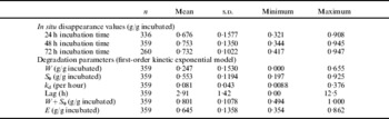
The data set used in the current study covers a large variety of forages with different botanical composition (grasses and legumes), types of forage (herbage, hay and silage) and maturity stage (cut after primary growth or after regrowth). This diversity resulted in wide ranges of values of parameters (Table 1) such as fractional degradation rate (ranging from 0·01 to 0·38), lag times (ranging from 0 to 12.5 h) and effective degradability (ranging from 0·35 to 0·86).

Degradable insoluble fraction S ₀

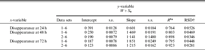
Asymptotic or potential degradability (W+S ₀) estimates obtained by fitting the exponential model were regressed against disappearance values at 24, 48 and 72 h (Table 2). The asymptotic value was strongly correlated (coefficient of correlation always higher than 0·87, P<0·001) with disappearance values at 24, 48 and 72 h. The prediction of (W+S ₀) from disappearance values was improved as the incubation time became longer, but in all cases there was underestimation of W+S ₀, based on the values of the intercept of the regression equations (Table 2). In the data sets used in the current study there were no disappearance data from long incubation times that could be assumed to closely approximate asymptotic potential disappearance, so it was decided to use disappearance at each incubation time as the end point to calculate slope (D at 24, 48, 72 or 96 h) for the estimation of S ₀ (S ₀=D−W).

Table 1.

Statistics (total number of observations (n), mean, standard deviation (s.d.) and range) for the in situ disappearance values and degradation parameters across the six data sets used in the study

W=soluble fraction; S ₀=potentially degradable fraction; k _d=fractional degradation rate; Lag=lag time; W+S ₀=potential (asymptotic) degradability); E=effective degradability.

Table 2.

Relationship between asymptotic or potential degradability (W+S₀) estimated from the exponential model and disappearance values at 24, 48 and 72 h of incubation. Results were obtained using ordinary least squares

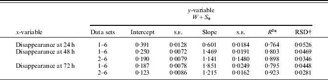
* R ²=variance accounted for (adjusted r ²).

† RSD=residual standard deviation.

Zero-order slope and lag

Slopes can be easily calculated using any incubation end point when lag time is assumed to be zero. Thus, initial points for the slope would be either (0, 0) or (0, W) (in the first case, it is assumed that W=0) and the end point can be any point with co-ordinates (t, D), where D is substrate disappearance at incubation time t. If L is known, slope can be calculated from (L, W) as the starting point. From the co-ordinates defined herein, the slopes of lines from (0, W) (no-lag-slope) and from (L, W) (lag-slope) are:

(10)

${\rm no {\hbox {-}} lag {\hbox {-}} slope} \equals {{D \minus W} \over t}$

(11)

${\rm lag {\hbox {-}} slope} \equals {{D \minus W} \over {t \minus L}}$

When only a few incubation points are used (as in the simplified procedure), lag (L) cannot be estimated or measured experimentally. Thus, slope from point (L, W) cannot be calculated as explained above. However, from Fig. 3, it can be seen that the slope from point (0, W) is geometrically related to the slope from (L, W):

${1 \over {{\rm lag {\hbox {-}} slope}}} \equals {1 \over {{\rm no {\hbox {-}} lag {\hbox {-}} slope}}} \minus {L \over {D \minus W}}$

and from Eqns (10) and (11), slope_ratio can be calculated as

(12)

${\rm slope}_{{\rm ratio}} \equals {\rm lag {\hbox {-}} slope \sol no {\hbox {-}} lag {\hbox {-}} slope} \equals {t \over {t \minus L}}$

Fig. 3.

Geometrical relationship between slopes from washout (0, W) and lag (L, W) points, where Z is the end point.

On the grounds of this geometrical relationship, it could be expected that both slopes (to the same end point) would be highly correlated and regression equations linking both variables can be derived:

${\rm lag {\hbox {-}} slope} \equals \alpha _{\rm L} \plus \beta _{\rm L} {\rm no {\hbox {-}} lag {\hbox {-}} slope}$

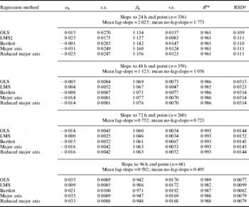
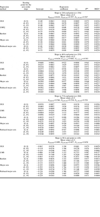
where α_L and β_L are the intercept and regression coefficient of the linear equation, respectively. As data sets used in the current work contained disappearance data at several incubation times for each feed studied, the exponential model was fitted and estimates of lag were obtained. These estimates were used to calculate lag-slopes and then, using all available pairs of no-lag- and lag-slopes, prediction equations of lag-slope from no-lag-slope were derived (Table 3). Lag-slope can be accurately predicted from no-lag-slope given the high coefficients of determination (R ²>0·96, P<0·001) and the low standard error of estimate (residual standard deviation). Standard errors of the parameter estimates are also small, with intercept values close to zero, and slopes close to unity.

Table 3.

Relationships between the zero-order slope from the lag point (L, W) (see Fig. 2) and the corresponding zero-order no-lag-slope from the point (0, W), both to the same incubation end point (24, 48, 72 or 96 h), after fitting the linear equation: lag-slope=α_L+β_L no-lag-slope. Results were obtained using OLS, robust regression or some Type II regression models to account for measurement errors in the predictor variables

* R ²=variance accounted for (adjusted r ²).

† RSD=residual standard deviation.

‡ LMS: this method removes outliers; hence R ² and RSD are based on the reduced data set.

Once estimates of α_L and β_L are obtained by linear regression, slope_ratio can be calculated:

${\rm slope}_{{\rm ratio}} \equals \beta _{\rm L} \plus {{\alpha _{\rm L} } \over {{\rm no {\hbox {-}} lag {\hbox {-}} slope}}}$

Using predicted lag-slopes and slope_ratio, lag time (L) can be calculated. Thus, from Eqn (12):

$L \equals {{t\lpar {\rm slope}_{{\rm ratio}} \minus 1\rpar } \over {{\rm slope}_{{\rm ratio}} }}$

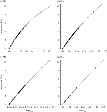
Using actual slope_ratio from the six data sets showed that the above algebra reproduced the estimated lag values accurately. Clearly, lag predictions depend on the quality of the relationship between lag-slope and no-lag-slope. However, the relationship between lag L and slope_ratio is curvilinear (Fig. 4), and can be modelled according to a simple exponential equation of the form $L \equals \alpha ^\prime \minus \beta ^\prime {\rm e}^{ \minus \kappa {\rm slope}_{{{\rm ratio}}} }$ , where α′, β′ and κ are constants. The upper asymptote of this relationship will be well outside the data range (Fig. 4), but this does not matter as only predictions from the overall equation in the range 0⩽L<10 are of interest. Fitted equations (using bootstrapping) for prediction of L from slope_ratio (calculated at end points 24, 48, 72 and 96 h) were as follows:

$\eqalign{\tab \hskip-48pt{\rm End\ point\ 24\ h\colon } \hfill\cr L \equals\tab 14{\cdot} 34\lpar 0{\cdot} 214\rpar \minus 73{\cdot} 53\lpar 1{\cdot} 118\rpar\hfill\cr\tab\times\exp \lsqb \minus 1{\cdot} 6351\lpar 0{\cdot} 0300\rpar {\rm slope}_{{\rm ratio}} \rsqb. }$

$\openup1\eqalign{\tab \hskip-46pt\hfill{\rm End\ point\ 48\ h\colon }\hfill \cr\hfill L \equals\tab 26{\cdot} 25\lpar 0{\cdot} 219\rpar \minus 161{\cdot} 63\lpar 1{\cdot} 421\rpar\hfill \cr\tab\hfill\times\exp \lsqb \minus 1{\cdot} 8176\lpar 0{\cdot} 01709\rpar {\rm slope}_{{\rm ratio}} \rsqb.\hfill}$

$\openup1\eqalign{\hfill\tab \hskip-30pt{\rm End\ point\ 72\ h\colon }\hfill \cr \tab\hfill L \equals 38{\cdot} 39\lpar 0{\cdot} 167\rpar \minus 249{\cdot} 17\lpar 1{\cdot} 120\rpar\hfill \cr\tab\hfill\quad\ \ \times\exp \lsqb \minus 1{\cdot} 8703\lpar 0{\cdot} 00882\rpar {\rm slope}_{{\rm ratio}} \rsqb .\hfill}$

$\openup1\eqalign{\hfill\tab\hskip-30pt {\rm End\ point\ 96\ h\colon }\hfill \cr \tab\hfill L \equals 50{\cdot} 43\lpar 0{\cdot} 826\rpar \minus 337{\cdot} 96\lpar 6{\cdot} 331\rpar\hfill \cr\tab\hfill\quad\ \ \times\exp \lsqb \minus 1{\cdot} 9023\lpar 0{\cdot} 03479\rpar {\rm slope}_{{\rm ratio}} \rsqb .\hfill }$

Fig. 4.

Relationship between lag time and slope_ratio (ratio between slope (lag-slope) from the lag point (L, W) and the corresponding slope (no-lag-slope) from the point (0, W), both to the same incubation end point (24, 48, 72 or 96 h); i.e. slope_ratio=lag-slope/no-lag-slope) at several incubation times (see text and Fig. 3 for details).

With this approach, it is possible to predict both zero-order lag-slope and L, which can be used subsequently for calculation of E.

Ruminal effective degradability

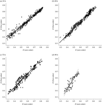
The reference data for effective degradability (E _exp) were calculated from the first-order exponential model as described by Dhanoa et al. (Reference Dhanoa, France, Siddons, López and Buchanan-Smith1995). Then E values were estimated using the simplified procedure developed herein by assuming zero-order kinetics. Slopes calculated from three different starting points ((0, 0); (0, W) and (L, W)) and to different incubation end points (24, 48, 72 and 96 h) were used for the calculation of E, giving 12 different estimates of effective degradability (E _(0,0)-24, E _(0,W)-24, E _(L,W)-24; E _(0,0)-48, E _(0,W)-48, E _(L,W)-48; E _(0,0)-72, E _(0,W)-72, E _(L,W)-72; E _(0,0)-96, E _(0,W)-96, E _(L,W)-96). In each case, corresponding values of W, L and S ₀ were used for the calculation of E according to Eqn (9). The calibration equations of E _exp (reference values) v. the 12 different estimates of effective degradability E (estimated values using zero-order kinetics) from the above regression methods are given in Table 4. All these equations were verified using the bootstrap method (1000 re-samples; Efron & Tibshirani Reference Efron and Tibshirani1993), as in some cases standard errors, R ² or residual standard deviation could not be calculated with the standard algorithm. All the equations for end points 24, 48 and 72 h accounted for over 0·91 of the variability in E _exp and it seems they are viable alternatives. With slopes up to incubation times of 24 h, slopes of the linear equations ranged between 0·81 and 0·89, and the intercept was between 0·123 and 0·149, whereas when slopes up to incubation times of 48 or 72 h were used, the regression coefficients of the calibration equations were close to unity and intercepts were in general smaller. The close relationship between estimated values (using different zero-order slopes from (0, W) to 24, 48, 72 and 96 h) and reference values (E _exp) is shown in Fig. 5. The small distances between the data points and the fitted line are noticeable, as well as the narrow confidence interval through the range of the values of E used in the study.

Fig. 5.

Relationship between values of effective degradability calculated with the reference method (E (first order)) and those calculated with the simplified procedure (E (zero order)) using slopes from washout point (0, W) to different incubation time end points. (The solid line is the geometric mean, the broken lines are the upper and lower limits, and the number in each point represents the data set from which the point is originated.)

Table 4.

Relationship between values of effective degradability (E) in the rumen (for a fractional rate of passage=0·02/h) calculated either by fitting the exponential model (first-order kinetics) to serial in situ disappearance data (considered as reference values (dependent or predicted variable) with mean across all data sets=0·645 ranging between 0·354 and 0·862, s.d.=0·136, n=360) or by assuming zero-order kinetics and using the simplified procedure (with slopes from origin (0, 0), washout point (0, W) or lag point (L, W) and to different end points (24, 48, 72 or 96 h of incubation), resulting in the different explanatory variables (three for each end point)). Results were obtained using OLS, robust regression or some Type II regression models to account for measurement errors in the predictor variables. All regressions were performed using bootstrapping

* R ²=variance accounted for (adjusted r ²).

† RSD=residual standard deviation.

‡ LMS: this method removes outliers; hence R ² and RSD are based on the reduced data set.

All regression methods yielded similar results, with some particularities in their behaviour. The LMS method, which enhanced R ² and reduced RSD but increased standard errors of the parameters (as fewer points are used in the regression), was found to be computationally demanding and it also appears to eliminate some data that are difficult to consider as true outliers. Bartlett's 3-Group Method is clearly unsuitable if the sample size is small, although it shows acceptable performance for larger samples. The reduced major axis method (the familiar Y on X and X on Y procedure when both X and Y are subject to measurement error) and the major axis method performed equally well. Due to high correlations, OLS results are very similar to corresponding results from Type II regression methods. This will not be the case if the correlation is relatively poor. For example, the slope from the reduced major axis method will be higher by a factor of 1/r (where r is the Pearson correlation coefficient) when compared with the slope from OLS.

Results for the 96 h end point are given for completeness only, because its choice is contrary to the objective of the current study. Due to lack of data and perhaps structural matrix collapse, 96 h end point does not appear to be an option.

Validation

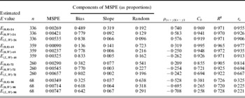
Mean square prediction error (MSPE) (Bibby & Toutenburg Reference Bibby and Toutenberg1977; Dhanoa et al. Reference Dhanoa, Lister, France and Barnes1999b) analyses were performed on the differences between values of effective degradability in the rumen (E; k _p=0·02/h) calculated from the first-order exponential model (considered as reference values) and corresponding zero-order estimates using slopes from three different starting points ((0, 0), (0, W) and (L, W)) and to different incubation end points (24, 48, 72 and 96 h). Concordance correlation coefficient (r _c) was used to evaluate reproducibility of the reference E values from the predicted E values (r _c; Lin Reference Lin1989; Dhanoa et al. Reference Dhanoa, Lister, France and Barnes1999b). This is an index of how far the observations deviate from the concordance line (departure from standard), by multiplying a measure of precision (deviation from the best-fit line measured by the Pearson correlation coefficient r) by a measure of accuracy (deviation, i.e. displacement and rotation, of the best-fit line from the 1:1 concordance or equality line). This index of accuracy is termed C _b (C _b=r _c/r). To test the equality of variance of actual and corresponding predicted values, ‘sum and product’ correlation (ρ_(x+y)(x₋_y ₎; Morgan Reference Morgan1939; Pitman Reference Pitman1939; Dhanoa et al. Reference Dhanoa, Lister, France and Barnes1999b) was calculated. These results from the above analyses are summarized in Table 5. Mean bias and slope bias are for the calibration equations given in Table 4.

Table 5.

Mean square prediction error (MSPE) breakdown of differences between estimates of effective degradability in the rumen (E) from the first-order kinetic exponential model (considered as reference values) and corresponding zero-order kinetic estimates E _(x,y)-t, where (x, y) are the coordinates of the starting point and t is the end-incubation time for the calculation of the zero-order slope

ρ_(x+y)(x_−y)=product moment correlation between x+y and x–y (all values of this statistic were significant, P<0·001).

C _b=index of accuracy for relationship drift away from the 1:1 line.

r _c=Lin's concordance correlation.

Further, to test the performance of relationships in Table 4, each of the six sets was in turn considered as the validation set. The equations in Table 4 were recalculated for the remaining five sets and predictions for the chosen validation set were made. MPSE analyses were performed on the actual v. corresponding predicted values for the relevant set and also overall (results not shown). The ‘sum and product’ correlation ρ_(x+y)(x₋_y ₎ was shown not to be significant overall (except 96 h end point) although for individual sets some significant results were observed. It would appear that a good calibration data set can provide equations capable of giving acceptable predictions, thus avoiding the laborious full in situ procedure and sparing donor animals much of the impact.

DISCUSSION

Calibration equations have been developed to predict effective degradability of feeds, in particular forages, in the rumen (reference values estimated from the simple exponential model based on first-order kinetics) using the simplified procedure developed herein assuming zero-order kinetics. Statistics used to assess goodness-of-fit and to examine prediction errors of these equations have shown that the simplified procedure is a viable alternative to the standard in situ one.

The simplified procedure proposed involved a two-stage mathematical process, with statistical prediction of some parameters (such as lag time or S ₀ fraction) and then application of a kinetic model (derived by assuming degradation follows zero-order kinetics) to determine E from the predicted parameters. The main advantage of the proposed procedure is that it can be applied with just one incubation time (end points 24, 48 or 72 h). The wash fraction (determined by washing bags containing the sample without previous incubation in the rumen) can be incorporated in the modelling, although it may be assumed to be zero. The lag time can be estimated and slopes from the point (L, W) predicted if slopes from the point (0, W) are known, as regression equations have been derived from the geometrical relationship between both slopes. Fraction S ₀ (insoluble but potentially degradable) can be determined, but it has also been demonstrated that it may be calculated from disappearance values at the incubation end point used in each case. Although values of S ₀ calculated are highly variable depending on the incubation end point (greater disappearance and S ₀ values as the incubation time becomes longer), this did not result in higher estimates of effective degradability when longer end-incubation times were used for the calculation of the zero-order slope and S ₀ (Table 4). Zero-order slope would be higher if shorter incubation times are used as end points, thus compensating for the smaller S ₀ values. Therefore, the approach using just one incubation time for the calculation of both the zero-order slope and S ₀ seems to be valid to obtain approximate estimates of effective degradability. Finally, a linear slope from any initial point (0, 0) (0, W) or (L, W) and to a given end point (disappearance at 24, 48 or 72 h) can easily be calculated and used to determine E by applying the equation derived for zero-order kinetics. The current results have shown that with any starting point and end points of 24, 48 or 72 h it is possible to obtain accurate estimates of E values that can be used in feed formulation for ruminants. E values from the simplified method rank feedstuffs in a similar order to the values obtained from the exponential model and average values from both approaches are similar to each other. For further refinement, prediction equations for effective degradability have been developed by regressing E _exp on E calculated from the simplified method, allowing for mathematical adjustments.

Predictive equations were derived from six different data sets and using diverse forages. The possible influence of a particular data set or type of forage on the estimates of the equation parameters (intercept and slope) was examined using generalized linear models in which the significance of effects attributed to blocking factors (such as data set or type of forage) was tested, confirming that the contribution of these blocking factors to the variance accounted for in the predictive models was of rather little significance. With the experimental design used herein, such effects were not expected because predicted (reference E value) and explanatory (zero kinetic E values) were obtained from paired and matching calculations using the same data for each in situ disappearance curve within all the structural factors in the database used.

In general, fitting the well-known exponential model (based on first-order kinetics) to serial disappearance data using non-linear regression has been considered as the standard method for estimating E. The main inconvenience of this method is that several data points (at different incubation times) are required; hence some simplified procedures have been described in which reduced ruminal incubation times are used. Broderick (Reference Broderick and Fahey1994) proposed a procedure to calculate fractional degradation rate by log transformation of substrate disappearance percentages at only two incubation times (0 and 16 h). Then, with this degradation rate effective degradability could be determined, resulting in estimates of protein degradability similar to those calculated with time-course data. Vanzant et al. (Reference Vanzant, Cochran, Titgemeyer, Stafford, Olson, Johnson and St Jean1996) confirmed the validity of this procedure to estimate degradability of forages. Calsamiglia et al. (Reference Calsamiglia, Yoon and Stern1994) used a similar double-point approach (changing the incubation times) to estimate protein degradability and obtained values close to those observed with the standard procedure. Wilkerson et al. (Reference Wilkerson, Klopfenstein and Stroup1995) assumed that disappearance at 16 h was an acceptable approximation to protein degradability of roughages. More recently, Olaisen et al. (Reference Olaisen, Mejdell, Volden and Nesse2003) developed multiple regression equations to estimate degradability from in situ disappearance values using only two or three incubation times. This approach is rather empirical, based on the statistical relationship between the variables, but Olaisen et al. (Reference Olaisen, Mejdell, Volden and Nesse2003) claimed that the procedure was more robust and less vulnerable than previous approaches, because estimation of degradation rates was highly dependent on errors in the disappearance values.

A feature of the simplified procedure derived herein is the combination of statistical and kinetic models. Some parameters are estimated from prediction equations and then a kinetic model is used to calculate effective degradability. The kinetic model assumes that degradation obeys zero-kinetics, i.e. the degradation rate is constant. In the case of degradation obeying zero-kinetics, the plot of disappearance v. incubation time is represented by a straight line, whose slope can be estimated from just two data-points. It was shown that values calculated from this approach were similar to those obtained with the reference method, even though a wide range of initial and end points of incubation were used to test the procedure. Changing incubation points resulted in major differences in the zero-order slopes (degradation rate) calculated, but in all cases estimates of E were similar and approximated the reference values. A piecewise segmented model with three straight lines representing zero-order kinetics has been fitted to in situ disappearance profiles to estimate degradation parameters and effective degradability in the rumen. E values with this segmented model slightly overestimated the values determined with the exponential model, although differences can be considered to be of little significance (López et al. Reference López, France, Dhanoa, Mould and Dijkstra1999; Fathi Nasri et al. Reference Fathi Nasri, Danesh Mesgaran, France, Cant and Kebreab2006; Nivyobizi et al. Reference Nivyobizi, Deswysen, Moreau, Dehareng, Larondelle and Peeters2007).

Along with the high degree of precision and accuracy attained in the prediction of E, the simplified procedure involves a number of important methodological benefits. As both the number of incubation times and the total incubation time required are reduced, the impact of incubation of artificial fibre bags in the rumen will be significantly decreased. Increase in capacity will be considerable, allowing a sizable reduction in the time required to process a large number of test substrates. Also, shorter incubation periods should minimize day-to-day variability. In order to address quality assurance and standardization issues, it may be prudent to include some standard or reference samples for which E will be determined by both the simplified and the standard (full in situ degradation curve) procedures. The validation of equations in Table 4, over the six data sets in the current study, has been satisfactory but further validation outside of these data sets should confirm and corroborate findings from the current study.

CONCLUSIONS

Effective degradability of feeds in the rumen can be accurately estimated using the simplified approach developed herein. Only disappearance values at one incubation time (24, 48 or 72 h) are required. In a first stage, certain parameters (e.g. lag time) are determined using prediction equations. Then a kinetic model, which assumes that degradation in the rumen is a zero-order kinetic process, is used to calculate degradability. There is a high degree of reproducibility of the reference values, indicating that loss of accuracy using the simplified procedure is of little nutritional significance. On the contrary, fewer incubation times entail reduced human labour and impact of the in situ procedure on the host animals. Increased capacity, operational advantages and animal welfare issues point to the use and adoption of this alternative way of conducting in situ studies.

This research was funded, in part, by the Canada Research Chairs Programme.

Footnotes

†

Merged into The Institute of Biological, Environmental and Rural Sciences (IBERS), Aberystwyth University.

References

REFERENCES

Bartlett, M. S. (1949). Fitting a straight line when both variables are subject to error. Biometrics 5, 207–212.CrossRef Google Scholar

Beever, D. E., Dhanoa, M. S., Losada, H. R., Evans, R. T., Cammell, S. B. & France, J. (1986). The effect of forage species and stage of harvest on the processes of digestion occurring in the rumen of cattle. British Journal of Nutrition 56, 439–454.CrossRef Google Scholar PubMed

Bibby, J. & Toutenberg, H. (1977). Prediction and Improved Estimation in Linear Models. London: John Wiley and Sons.Google Scholar

Broderick, G. A. (1994). Quantifying forage protein quality. In Forage Quality, Evaluation, and Utilization (Ed. Fahey, G. C. Jr), pp. 200–228. Madison, WI: American Society of Agronomy, Crop Science Society of America and Soil Science Society of America.Google Scholar

Calsamiglia, S., Yoon, I. K. & Stern, M. D. (1994). Effect of various incubation times on in situ estimation of ruminal crude protein degradation. Journal of Animal Science 72 (Suppl. 1), 171.Google Scholar

Dhanoa, M. S. (1988). On the analysis of dacron bag data for low degradability feeds. Grass and Forage Science 43, 441–444.Google Scholar

Dhanoa, M. S., France, J., Siddons, R. C., López, S. & Buchanan-Smith, J. G. (1995). A nonlinear compartmental model to describe forage degradation kinetics during incubation in polyester bags in the rumen. British Journal of Nutrition 73, 3–15.Google Scholar

Dhanoa, M. S., France, J., López, S., Dijkstra, J., Lister, S. J., Davies, D. R. & Bannik, A. (1999 a). Correcting the calculation of extent of degradation to account for particulate matter loss at zero time when applying the polyester bag method. Journal of Animal Science 77, 3385–3391.CrossRef Google Scholar PubMed

Dhanoa, M. S., Lister, S. J., France, J. & Barnes, R. J. (1999 b). Use of mean square prediction error analysis and reproducibility measures to study near infrared calibration equation performance. Journal of Near Infrared Spectroscopy 7, 133–143.Google Scholar

Efron, B. & Tibshirani, R. J. (1993). An Introduction to the Bootstrap. London: Chapman and Hall.CrossRef Google Scholar

Fathi Nasri, M. H., Danesh Mesgaran, M., France, J., Cant, J. P. & Kebreab, E. (2006). Evaluation of models to describe ruminal degradation kinetics from in situ ruminal incubation of whole soybeans. Journal of Dairy Science 89, 3087–3095.CrossRef Google Scholar

France, J., Thornley, J. H. M., López, S., Siddons, R. C., Dhanoa, M. S., Van Soest, P. J. & Gill, M. (1990). On the two compartment model for estimating the rate and extent of feed degradation in the rumen. Journal of Theoretical Biology 146, 269–287.CrossRef Google Scholar PubMed

France, J., Dijkstra, J., Dhanoa, M. S., López, S. & Bannink, A. (2000). Estimating the extent of degradation of ruminant feeds from a description of their gas production profiles observed in vitro: derivation of models and other mathematical considerations. British Journal of Nutrition 83, 143–150.Google Scholar

Leroy, A. & Rousseeuw, P. (1984). PROGRESS: A Program for Robust Regression. Technical Report 201. Brussels, Belgium: Center for Statistics and Operations Research, University of Brussels.Google Scholar

Lin, L. I. K. (1989). A concordance correlation coefficient to evaluate reproducibility. Biometrics 45, 255–268.Google Scholar

López, S. (2005). In vitro and in situ techniques for estimating digestibility. In Quantitative Aspects of Ruminant Digestion and Metabolism, 2nd edn (Eds Dijkstra, J., Forbes, J. M. & France, J.), pp. 87–121. Wallingford, UK: CAB International.CrossRef Google Scholar

López, S., Carro, M. D., González, J. S. & Ovejero, F. J. (1991 a). Rumen degradation of the main forage species harvested from permanent mountain meadows in North-western Spain. Journal of Agricultural Science, Cambridge 117, 363–369.CrossRef Google Scholar

López, S., Carro, M. D., González, J. S. & Ovejero, F. J. (1991 b). The effect of method of forage conservation and harvest season on the degradation of forages harvested from permanent mountain meadows. Animal Production 53, 177–182.Google Scholar

López, S., France, J., Dhanoa, M. S., Mould, F. & Dijkstra, J. (1999). Comparison of mathematical models to describe disappearance curves obtained using the polyester bag technique for incubating feeds in the rumen. Journal of Animal Science 77, 1875–1888.Google Scholar

McDonald, I. (1981). A revised model for the estimation of protein degradability in the rumen. Journal of Agricultural Science, Cambridge 96, 251–252.CrossRef Google Scholar

Mertens, D. R. (2005). Rate and extent of digestion. In Quantitative Aspects of Ruminant Digestion and Metabolism, 2nd edn (Eds Dijkstra, J., Forbes, J. M. & France, J.), pp. 13–47. Wallingford, UK: CAB International.CrossRef Google Scholar

Morgan, W. A. (1939). A test for the significance of the difference between the two variances in a sample from a normal bivariate population. Biometrika 31, 13–19.Google Scholar

Nivyobizi, A., Deswysen, G., Moreau, B., Dehareng, D., Larondelle, Y. & Peeters, A. (2007). The choice of a fitting model for in sacco degradation curves of some temperate and tropical grasses. Grass and Forage Science 62, 198–207.CrossRef Google Scholar

Olaisen, V., Mejdell, T., Volden, H. & Nesse, N. (2003). Simplified in situ method for estimating ruminal dry matter and protein degradability of concentrates. Journal of Animal Science 81, 520–528.Google Scholar

Ørskov, E. R. & McDonald, I. (1979). The estimation of protein degradability in the rumen from incubation measurements weighted according to rates of passage. Journal of Agricultural Science, Cambridge 92, 449–503.CrossRef Google Scholar

Pitman, E. J. G. (1939). A note on normal correlation. Biometrika 31, 9–12.Google Scholar

Rousseeuw, P. J. (1984). Least median squares regression. Journal of the American Statistical Association 79, 871–880.Google Scholar

Rousseeuw, P. J. & Leroy, A. M. (1987). Robust Regression and Outlier Detection. New York: Wiley.CrossRef Google Scholar

Sokal, R. R. & Rohlf, F. J. (1995). Biometry, 3rd edn. New York: W.H. Freeman.Google Scholar

Vanzant, E. S., Cochran, R. S., Titgemeyer, E. C., Stafford, S. D., Olson, K. C., Johnson, D. E. & St Jean, G. (1996). In vivo and in situ measurements of forage protein degradation in beef cattle. Journal of Animal Science 74, 2773–2784.CrossRef Google Scholar PubMed

Wilkerson, V. A., Klopfenstein, T. J. & Stroup, W. W. (1995). A collaborative study of in situ forage protein degradation. Journal of Animal Science 73, 583–588.CrossRef Google Scholar PubMed

Fig. 1.Feed fractions showing their degradation and passage kinetics in the rumen.

Fig. 2.Geometry of zero-order slopes from origin (0, 0), washout (0, W) and lag (L, W) points (Z is the chosen end point) in relation to the conceptualized first-order kinetics.

Table 1.Statistics (total number of observations (n), mean, standard deviation (s.d.) and range) for the in situ disappearance values and degradation parameters across the six data sets used in the study

Table 2.Relationship between asymptotic or potential degradability (W+S0) estimated from the exponential model and disappearance values at 24, 48 and 72 h of incubation. Results were obtained using ordinary least squares

Fig. 3.Geometrical relationship between slopes from washout (0, W) and lag (L, W) points, where Z is the end point.

Table 3.Relationships between the zero-order slope from the lag point (L, W) (see Fig. 2) and the corresponding zero-order no-lag-slope from the point (0, W), both to the same incubation end point (24, 48, 72 or 96 h), after fitting the linear equation: lag-slope=αL+βL no-lag-slope. Results were obtained using OLS, robust regression or some Type II regression models to account for measurement errors in the predictor variables

Fig. 4.Relationship between lag time and sloperatio (ratio between slope (lag-slope) from the lag point (L, W) and the corresponding slope (no-lag-slope) from the point (0, W), both to the same incubation end point (24, 48, 72 or 96 h); i.e. sloperatio=lag-slope/no-lag-slope) at several incubation times (see text and Fig. 3 for details).

Fig. 5.Relationship between values of effective degradability calculated with the reference method (E (first order)) and those calculated with the simplified procedure (E (zero order)) using slopes from washout point (0, W) to different incubation time end points. (The solid line is the geometric mean, the broken lines are the upper and lower limits, and the number in each point represents the data set from which the point is originated.)

Table 4.Relationship between values of effective degradability (E) in the rumen (for a fractional rate of passage=0·02/h) calculated either by fitting the exponential model (first-order kinetics) to serial in situ disappearance data (considered as reference values (dependent or predicted variable) with mean across all data sets=0·645 ranging between 0·354 and 0·862, s.d.=0·136, n=360) or by assuming zero-order kinetics and using the simplified procedure (with slopes from origin (0, 0), washout point (0, W) or lag point (L, W) and to different end points (24, 48, 72 or 96 h of incubation), resulting in the different explanatory variables (three for each end point)). Results were obtained using OLS, robust regression or some Type II regression models to account for measurement errors in the predictor variables. All regressions were performed using bootstrapping

Table 5.Mean square prediction error (MSPE) breakdown of differences between estimates of effective degradability in the rumen (E) from the first-order kinetic exponential model (considered as reference values) and corresponding zero-order kinetic estimates E(x,y)-t, where (x, y) are the coordinates of the starting point and t is the end-incubation time for the calculation of the zero-order slope

Article contents

Simplified estimation of forage degradability in the rumen assuming zero-order degradation kinetics

Summary

Information

INTRODUCTION

MATERIALS AND METHODS

General scheme

Mathematical formulation

Zero-order degradation

Simplified procedure

Data sets

Regression methods

RESULTS

Data set

Degradable insoluble fraction S 0

Zero-order slope and lag

Ruminal effective degradability

Validation

DISCUSSION

CONCLUSIONS

Footnotes

References

REFERENCES

Save article to Kindle

Save article to Dropbox

Save article to Google Drive

Reply to: Submit a response

Your details

You have entered the maximum number of contributors

Conflicting interests

Degradable insoluble fraction S ₀