1. Introduction
Turbulence, jets, waves and vortices characterise planetary circulation. An essential member of this group is the zonal flow (jets), especially in Jovian atmospheres such as those of Jupiter and Saturn. Moving along the east–west direction, the strength of zonal flows varies with latitude, but the strongest ones are located near the equatorial region. The strength of zonal flow depends on the underlying turbulence that generates it. In many turbulent flow cases, the energy is transferred from large to small scales; however, in the geophysical context, large-scale circulations emerge as a consequence of an upscale transfer/inverse cascade in certain two-dimensional quasi-geostrophic limits. Early studies have shown that in the presence of the geophysical
 $\beta$
-effect, closely packed eddies transform to zonally elongated structures (Rhines Reference Rhines1975). This hypothesis was extended to account for flows on Jovian planets under barotropic and baroclinic set-ups (Williams Reference Williams1978, Reference Williams1979). The barotropic representation used implicit forcing to consider the baroclinic effects (Williams Reference Williams1978). Under conditions of extreme barotropisation, the flow transitions to zonostrophic turbulence characterised by alternating jets similar to those of Jupiter and Saturn (Galperin et al. Reference Galperin, Sukoriansky, Dikovskaya, Read, Yamazaki and Wordsworth2006; Sukoriansky et al. Reference Sukoriansky, Dikovskaya and Galperin2007, Reference Sukoriansky, Dikovskaya and Galperin2008). In contrast, the baroclinic set-up revealed that the jets always coexist with ambient eddies (Williams Reference Williams1979; Panetta Reference Panetta1993), a phenomenon common in Jovian atmospheres, especially on Jupiter. Further studies have also explored the effect of topography and large-scale circulations under the baroclinic set-up (Thompson Reference Thompson2010; Berloff et al. Reference Berloff, Karabasov, Farrar and Kamenkovich2011; Boland et al. Reference Boland, Thompson, Shuckburgh and Haynes2012; Chen & Kamenkovich Reference Chen and Kamenkovich2013). Barotropic and baroclinic models emphasised that zonal winds are manifestations of shallow layers forced by baroclinic instabilities and relied significantly on the two-dimensional quasi-geostrophic approximation.
Simultaneously, the deep convection model also became popular (Busse Reference Busse1976, Reference Busse1994). According to this model, a barotropic interior, caused by the homogenisation of entropy gradients due to interior convection, allows the formation of Taylor columns. The nonlinear interaction of these columns then generates equatorial and high-latitude zonal winds (Galperin & Read Reference Galperin and Read2019). Mathematically, this involves solving the three-dimensional governing differential equations with either the anelastic approximation (Jones, Kuzanyan & Mitchell Reference Jones, Kuzanyan and Mitchell2009; Gastine & Wicht Reference Gastine and Wicht2012; Heimpel, Gastine & Wicht Reference Heimpel, Gastine and Wicht2016) or the Boussinesq assumption (Aurnou & Olson Reference Aurnou and Olson2001; Christensen Reference Christensen2001, Reference Christensen2002; Heimpel, Aurnou & Wicht Reference Heimpel, Aurnou and Wicht2005; Nicoski, O’Connor & Calkins Reference Nicoski, O’Connor and Calkins2024) and rotation. The key governing parameters in such a system include Rayleigh number (
 ${\textit{Ra}}$
), Ekman number (
 ${\textit{Ek}}$
) and Prandtl number (
 ${\textit{Pr}}$
);
 ${\textit{Ra}}$
is the ratio of buoyancy force to viscous force,
 ${\textit{Ek}}$
measures the strength of viscous force over Coriolis force and
 ${\textit{Pr}}$
is the measure of momentum to thermal diffusivity. Additionally, the convective Rossby number (
 $Ro_c$
) measures buoyancy force compared with the Coriolis force. The spherical domain resembles the actual shape of a geophysical and planetary system; however, the formation of zonal flow in this domain is subject to the radius ratio and curvature affecting the accommodation of multiple jets at higher latitudes (Heimpel et al. Reference Heimpel, Aurnou and Wicht2005). This complexity can be overcome by employing the local plane layer model or the
 $f$
-plane model. This enables the study of such flows in the Cartesian domain (Pedlosky Reference Pedlosky2013), thus representing the flow at a specific latitude. Three-dimensional Rayleigh–Bénard convection (RBC; Ahlers, Grossmann & Lohse Reference Ahlers, Grossmann and Lohse2009) and its rotating counterpart (RRBC; Ecke & Shishkina Reference Ecke and Shishkina2023) in a Cartesian coordinate system have been studied extensively. We also employ this set-up and perform large-eddy simulations (LES) to understand the mechanism associated with zonal flows.
Busse (Reference Busse1994) performed numerical computations to show that in zonal flow, the mean component of the stream function is more significant than the fluctuating one; hence, the key to understanding the nature of zonal flow lies in finding how the mean flow originates in such systems. The experiments of Krishnamurti & Howard (Reference Krishnamurti and Howard1981) indicated that mean flow is driven by Reynolds stresses owing to the tilting of the thermal plumes and, hence, the mean flows are not externally but internally generated. The authors then supplemented their experimental findings with a truncated mathematical model of Howard & Krishnamurti (Reference Howard and Krishnamurti1986) (often referred to as the H-K model). These studies built the foundation for an in-depth investigation of shear-flow instability in RBC, resulting in numerous numerical and theoretical investigations on shear-flow instability in convective systems (Drake et al. Reference Drake, Finn, Guzdar, Shapiro, Shevchenko, Waelbroeck, Hassam, Liu and Sagdeev1992; Hermiz, Guzdar & Finn Reference Hermiz, Guzdar and Finn1995; Paparella & Spiegel Reference Paparella and Spiegel1999). More recently, it has been demonstrated that in low-order models, instability is suppressed in a large aspect ratio due to eddy–eddy nonlinear interactions (Fitzgerald & Farrell Reference Fitzgerald and Farrell2014). The studies used the flexibility of the low-order model rather than solving the full governing differential equation.
Goluskin et al. (Reference Goluskin, Johnston, Flierl and Spiegel2014), in a two-dimensional RBC set-up, studied zonal flow formation in the Cartesian domain by solving the full governing equations numerically. They reported that convection drives vertically sheared large-scale horizontal flow, the mean horizontal component of which was termed zonal flow. The associated shear of zonal flow disperses the convective structures to reduce heat transport. Simulations of zonal flow in such two-dimensional RBC are the limiting case of
 $Ek \rightarrow 0$
and neglect the effect of finite rotation.
The study of thermal convection in three-dimensional horizontally RRBC has attracted significant attention recently (Von Hardenberg et al. Reference Von Hardenberg, Goluskin, Provenzale and Spiegel2015; Wang et al. Reference Wang, Chong, Stevens, Verzicco and Lohse2020; Wang et al. Reference Wang, Wang, Wan and Sun2021; Lüdemann & Tilgner Reference Lüdemann and Tilgner2022). Similar to the two-dimensional studies (Goluskin Reference Goluskin2013; Goluskin et al. Reference Goluskin, Johnston, Flierl and Spiegel2014), zonal flow in three dimensions forms after convective rolls annihilate. Von Hardenberg et al. (Reference Von Hardenberg, Goluskin, Provenzale and Spiegel2015) showed that comparably strong winds can also develop in three-dimensional RBC at
 $Ra = 10^7$
with finite background rotation about a horizontal axis. With horizontal rotation, the flow resembles that near the equator in a typical
 $f$
-plane set-up (Pedlosky Reference Pedlosky2013), and latitudinal variation of the Coriolis force is excluded. Lüdemann & Tilgner (Reference Lüdemann and Tilgner2022) performed numerical simulations to infer that two-dimensional convection rolls aligned parallel to the rotation axis become unstable to three-dimensional disturbances owing to elliptical instability. Direct numerical simulations (DNS) of three-dimensional horizontally RRBC at
 $Ra = 10^7$
were performed by Wang et al. (Reference Wang, Chong, Stevens, Verzicco and Lohse2020) to study the transition of zonal flow to convection rolls for different aspect ratios at
 $Ra = 10^7$
. However, unlike Von Hardenberg et al. (Reference Von Hardenberg, Goluskin, Provenzale and Spiegel2015), Wang et al. (Reference Wang, Chong, Stevens, Verzicco and Lohse2020) used a linear shear-flow profile as an initial condition for triggering the zonal flows. Similarly, Wang et al. (Reference Wang, Wang, Wan and Sun2021) used two different shear-flow profiles in their DNS to study the influence of aspect ratio on the flow states in RBC without rotation at
 $Ra=10^{8}$
. They found a shear-flow state with a primary balance between the buoyancy flux and the viscous dissipation, and a convective roll state with a balance between production and dissipation.
From the above discussion, it is apparent that the literature on three-dimensional zonal flows in horizontally RRBC is limited to moderate Ra of
 $10^7$
. Therefore, in this investigation, we (i) explore the existence and nature of zonal flows in previously unreported
 $Ra{-}Ek$
parameter space relevant to geophysically interesting regimes, (ii) ascertain the parameters over which zonal flows could be obtained in horizontal RRBC and (iii) quantitatively prove the presence of an upscale energy transfer in horizontal RRBC (Von Hardenberg et al. Reference Von Hardenberg, Goluskin, Provenzale and Spiegel2015). To achieve these objectives, we performed LES of horizontal RRBC over a range of
 ${\textit{Ra}}$
(
 $10^{7}$
to
 $10^{12}$
) and
 $1/Ro_c = 0.16852$
,
 $1.6852$
,
 $16.852$
and
 $168.52$
(signifying faster rotation rate in terms of
 ${\textit{Ek}}$
(
 $10^{-3}$
to
 $10^{-8}$
)). Here LES provides a suitable alternative to DNS (Von Hardenberg et al. Reference Von Hardenberg, Goluskin, Provenzale and Spiegel2015; Wang et al. Reference Wang, Chong, Stevens, Verzicco and Lohse2020, Reference Wang, Wang, Wan and Sun2021) to reach a very high
 ${\textit{Ra}}$
while using a relatively coarse grid. Some existing work has utilised LES for simulating RBC without rotation (Kimmel & Domaradzki Reference Kimmel and Domaradzki2000; Peng, Hanjalic & Davidson Reference Peng, Hanjalic and Davidson2006), but the utilisation of LES for RRBC remains unreported. We study the transition of convective rolls to zonal flow without imposing any shear profile as an initial condition (Wang et al. Reference Wang, Chong, Stevens, Verzicco and Lohse2020). The evolution of the Reynolds number based on the mean kinetic energy and the turbulent kinetic energy demonstrates the advent of a zonal flow, further implying a gain of energy in the mean scales at the expense of turbulence. We calculate the total kinetic energy spectra and the vertically integrated energy flux to conclude that buoyancy deposits energy at small scales on the horizontal planes, from where it is transferred upscale. Many researchers have also investigated the energy and its flux in spectral space for RBC to study the upscale transfer and the inverse cascade mechanism. However, these studies created barotropic and baroclinic modes by taking averages along the vertical (Rubio et al. Reference Rubio, Julien, Knobloch and Weiss2014; Favier, Silvers & Proctor Reference Favier, Silvers and Proctor2014; Guervilly, Hughes & Jones Reference Guervilly, Hughes and Jones2014). We complete our understanding by analysing the force balance, fluctuating velocities and Reynolds stress, and present a comprehensive investigation of the evolution and dynamics of zonal flow.
We present the problem formulation, the governing equations, the geometrical set-up of the horizontal RRBC, the details of LES, the subgrid model, simulation cases and the averaging technique, followed by the solver validation in § 2. The results of our simulations are described in § 3, beginning with qualitative visualisation of the convective and zonal flow states, followed by turbulent statistics such as Reynolds number, energy spectra, turbulent kinetic energy (TKE) budgets and force balance. We conclude our findings in § 4.
Schematic of the horizontal RBC set-up. The bottom plate is at temperature
 $T_{h}$
and the top plate is at
 $T_{c}$
. The rotation vector is parallel to
 $x_{2}$
and gravity anti-parallel to
 $x_{3}$
, with dimensions
 $L_1=L_2$
 $=2\pi$
and
 $L_3=$
 $1$
.

2. Problem formulation
2.1. Governing equations
We consider the buoyant convection of an incompressible Boussinesq fluid between a hot (bottom) and cold (top) plate as shown in figure 1. With the temperature difference constantly maintained at
 $\Delta T$
, the system is subjected to background rotation
 $\varOmega$
=
 $\varOmega$
 $\hat {e_{2}}$
about the horizontal axis, perpendicular to gravity given by
g
=
 $-g$
 $\hat {e_{3}}$
. The fluid is Newtonian with density
 $\rho$
, kinematic viscosity
 $\nu$
, thermal diffusivity
 $\kappa$
and adiabatic volume expansion coefficient
 $\alpha$
. We select the vertical height
 $H$
, temperature difference
 $\Delta T$
and free-fall velocity
 $u_{f}=\sqrt {g\alpha \Delta T H}$
as the scales for length, temperature and velocity to non-dimensionalise the governing equations (Pandey, Scheel & Schumacher Reference Pandey, Scheel and Schumacher2018; Naskar & Pal Reference Naskar and Pal2022a
,
Reference Naskar and Palb
). The filtered non-dimensional governing equation (Pham & Sarkar Reference Pham and Sarkar2014b
) for LES takes the following form:
 \begin{align} &\qquad \qquad \qquad \frac {\partial \overline {u}_{\!j}}{\partial x_{\!j}} = 0, \end{align}
 \begin{align} \frac {\partial \overline {u}_{i}}{\partial t} + \frac {\partial \overline {u}_{\!j}\overline {u}_{i}}{\partial x_{\!j}}=& -\frac {\partial \overline {P}}{\partial x_{i}}+ \frac {2}{Ek}\sqrt {\frac {\textit{Pr}}{Ra}}\epsilon _{ij2}\overline {u}_{\!j} +\overline {\theta }\delta _{i3}+ \sqrt {\frac {\textit{Pr}}{Ra}}\frac {\partial ^2 \overline {u}_{i}}{\partial x_{\!j} \partial x_{\!j}} - \frac {\partial \tau _{ij}}{\partial x_{\!j}}, \end{align}
 \begin{align} &\frac {\partial \overline {\theta }}{\partial t} + \frac {\partial \overline {u}_{\!j}\overline {\theta }}{\partial x_{\!j}} = \frac {1}{\sqrt {\textit{RaPr}}}\frac {\partial ^2 \overline {\theta }}{\partial x_{\!j} \partial x_{\!j}} - \frac {\partial Q_{\!j}}{\partial x_{\!j}}, \end{align}
where the overbar denotes the filtered quantities. The non-dimensional parameters, namely the Rayleigh number (
 ${\textit{Ra}}$
), the Prandtl number (
 ${\textit{Pr}}$
) and the Ekman number (
 ${\textit{Ek}}$
), appearing in (2.1)–(2.3) are defined as follows:
 \begin{align} Ra=\frac {g\alpha \Delta T H^{3}}{\kappa \nu },\quad \textit{Pr}=\frac {\nu }{\kappa },\quad Ek=\frac {\nu }{\varOmega H^{2}}. \end{align}
The Rayleigh number (
 ${\textit{Ra}}$
) is the buoyancy and viscous force ratio, determining the turbulence intensity, which increases when
 ${\textit{Ra}}$
is increased. The Ekman number (
 ${\textit{Ek}}$
) measures the viscous force compared with the Coriolis force. Decreasing
 ${\textit{Ek}}$
implies increasing rotation rate. The Prandtl number (
 ${\textit{Pr}}$
) measures the momentum to thermal diffusivity ratio. In RRBC, the convective Rossby number (
 $Ro_c$
) measures the ratio of buoyancy force to Coriolis force. Here
 $Ro_c$
relates to the above-mentioned parameters as
 \begin{equation} \frac {1}{Ro_c} = \frac {2}{Ek}\sqrt {\frac {\textit{Pr}}{Ra}}=\frac {2\varOmega H}{u_f}. \end{equation}
We keep
 $\textit{Pr} =\,$
0.71 and select
 ${\textit{Ra}}$
and
 ${\textit{Ek}}$
to get a set of
 $1/Ro_c = 0.16852$
,
 $1.6852$
,
 $16.852$
and
 $168.52$
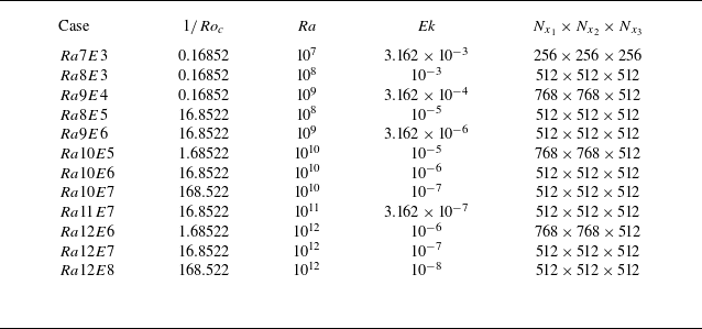
(see table 1). We use periodic boundary conditions in the horizontal directions (x
 $_{1}$
, x
 $_{2}$
), whereas to facilitate zonal flows we impose stress-free boundary conditions in the vertical direction similar to Von Hardenberg et al. (Reference Von Hardenberg, Goluskin, Provenzale and Spiegel2015) and Wang et al. (Reference Wang, Chong, Stevens, Verzicco and Lohse2020) as follows:
 \begin{align} \frac {\partial u_{1}}{\partial x_{3}}=\frac {\partial u_{2}}{\partial x_{3}}=u_{3}=0 \quad \mbox{at}\quad x_3=\pm \frac {1}{2}. \end{align}
For the temperature field, isothermal boundary conditions are applied on both the top and bottom plates to maintain an unstable temperature gradient as follows:
 \begin{align} \theta =0.5\quad \mbox{at}\quad x_{3}=-\frac {1}{2},\quad \theta =-0.5 \quad \mbox{at}\quad x_3=\frac {1}{2}. \end{align}
2.2. Large-eddy simulations and subgrid model
In LES, large scales are computed, whereas small scales are modelled. Any quantity in this context can be expressed as the sum of the resolved (filtered) and subgrid terms. In (2.1)–(2.3),
 $\tau _{ij}$
and
 $Q_{\!j}$
denote the subgrid stress and subgrid buoyancy flux, respectively, which arise owing to the filtering of the governing equations (Pham & Sarkar Reference Pham and Sarkar2014b
). We use the dynamic Smagorinsky model of Germano et al. (Reference Germano, Piomelli, Moin and Cabot1991) to perform the simulations in this investigation. The dynamic model has been successfully used to simulate different problems (Taylor & Sarkar Reference Taylor and Sarkar2007; Tejada-Martinez & Grosch Reference Tejada-Martinez and Grosch2007; Armenio & Sarkar Reference Armenio and Sarkar2002; Pham & Sarkar Reference Pham and Sarkar2014b
) relevant to geophysical flows. The subgrid stress and buoyancy flux are given by
 \begin{align} \tau _{ij} &=-2C_{d}\overline {\Delta }^{2}\lvert \overline {S}\rvert \overline {S}_{ij}, \end{align}
 \begin{align} Q_{\!j} &=-C_{T}\overline {\Delta }^{2}\lvert \overline {S}\rvert \frac {\partial \overline {\theta }}{\partial x_{\!j}}, \end{align}
where
 $\overline {\Delta }$
is the filter width,
 $\overline {S}$
 $_{ij}$
= 1/2(
 $\partial \overline {u}$
 $_{i}$
/
 $\partial {x_{\!j}}$
+
 $\partial \overline {u}$
 $_{\!j}$
/
 $\partial {x_{i}}$
) is the resolved strain rate tensor and
 $\lvert \overline {S}\rvert$
is defined as
 $\sqrt {2 \overline {S}_{ij}\overline {S}_{ij}}$
. The subgrid diffusivity is given by
 \begin{align} \nu _{\textit{sgs}} &=C_{d}\overline {\Delta }^{2}\lvert \overline {S} \rvert , \end{align}
 \begin{align} \kappa _{\textit{sgs}} &=C_{T}\overline {\Delta }^{2}\lvert \overline {S} \rvert. \end{align}
Following Germano et al. (Reference Germano, Piomelli, Moin and Cabot1991) and Lilly (Reference Lilly1992), the model coefficients are dynamically determined as follows:
 \begin{equation} C_{d}=-\frac {1}{2}\frac {\langle L_{ij}M_{ij} \rangle }{\langle M_{ij}M_{ij} \rangle }, \end{equation}
where
 \begin{align} L_{ij} &=\widetilde {\overline {u}_{i} \overline {u}_{\!j}}-\widetilde {\overline {u}_{i}}\widetilde {\overline {u}_{\!j}}, \end{align}
 \begin{align} M_{ij} &=\widetilde {\overline {\Delta }}^{2}\widetilde {\lvert \overline {S} \rvert }\widetilde {\overline {S}_{ij}} - \widetilde {\overline {\Delta }^{2}\lvert \overline {S} \rvert \overline {S}_{ij}}, \end{align}
and the dynamic coefficient for the subgrid buoyancy is given as
 \begin{equation} C_{T}=-\frac {1}{2}\frac {\langle L_{ij}^{T}M_{ij}^{T} \rangle }{\langle M_{ij}^{T}M_{ij}^{T} \rangle }, \end{equation}
where
 \begin{align} L_{i}^{T} &= \widetilde {\overline {\theta }\overline {u}_{i}}-\widetilde {\overline {\theta }}\widetilde {\overline {u}_{i}}, \end{align}
 \begin{align} M_{i}^{T} &= \widetilde {\overline {\Delta }}^{2}\widetilde {\lvert \overline {S} \rvert }\widetilde {\frac {\partial \overline {\theta }}{\partial x_{i}}} - \widetilde {\overline {\Delta }^{2}\lvert \overline {S} \rvert \frac {\partial \overline {\theta }}{\partial x_{i}}}. \end{align}
The test filter is applied using an explicit three-point trapezoidal rule. The value of
 $\widehat {\overline {\Delta }}$
/
 $\overline {\Delta }$
is generally taken as
 $\sqrt {6}$
(Pham & Sarkar Reference Pham and Sarkar2014b
) and
 $\langle \cdots\rangle$
denotes averaging in the homogeneous direction (horizontal
 $x_1{-}x_2$
direction in our case). The
 $\widetilde {\overline {\phi }}$
implies double filtering of any quantity
 $\phi$
, first with the grid/LES filter, followed by the test filter. This is done to smooth out the large pointwise variations in the coefficients. Positive coefficients imply the model is purely dissipative, and energy is transferred from resolved to subgrid scales. In cases where
 $C_{d}$
and
 $C_{\theta }$
become negative, they are clipped to zero to prevent numerical instability (Pham & Sarkar Reference Pham and Sarkar2014b
).
2.3. Numerical details and validation
For any quantity
 $\phi$
, the Reynolds decomposition is given by
 \begin{equation} \phi (x_{1},x_{2},x_{3},t) = \langle \phi \rangle (x_{3},t) + \phi ^{\prime }(x_{1},x_{2},x_{3},t), \end{equation}
where the horizontal average (denoted by
 $\langle \cdots \rangle$
) is defined as
 \begin{equation} \langle \phi \rangle (x_{3},t) = \frac {1}{L_{1}}\frac {1}{L_{2}} \int _{-L_{1}/2}^{L_{1}/2} \int _{-L_{2}/2}^{L_{2}/2} \phi \, {\rm d}x_{1}{\rm d}x_{2}. \end{equation}
All the flow variables
 $\overline {u}_{1}$
,
 $\overline {u}_{2}$
,
 $\overline {u}_{3}$
,
 $\overline {\theta }$
and other turbulent quantities (§ 3) are decomposed according to (2.18)–(2.19) to study their statistics. The governing equations are solved using the finite difference method (Bakhuis et al. Reference Bakhuis, Ostilla-Mónico, Van Der Poel, Erwin, Verzicco and Lohse2018) in a staggered grid arrangement. The scalar quantities (pressure and temperature) are stored at the cell centres, whereas the velocity components are stored at the cell faces. We use a second-order central difference scheme for spatial discretisation and the projection method to calculate the divergence-free velocity field, where the pressure Poisson equation is solved using a parallel multigrid algorithm. An explicit third-order Runge–Kutta method is used for time advancement, except for the diffusion terms, which are solved implicitly using the Crank–Nicolson method (Pham, Sarkar & Brucker Reference Pham, Sarkar and Brucker2009; Brucker & Sarkar Reference Brucker and Sarkar2010). The solver has been extensively used for studies on rotating stratified flow and various transitional and turbulent shear flows (Pal, de Stadler & Sarkar Reference Pal, de Stadler and Sarkar2013; Pal & Sarkar Reference Pal and Sarkar2015; Pal & Chalamalla Reference Pal and Chalamalla2020; Pal Reference Pal2020; Singh & Pal Reference Singh and Pal2023, Reference Singh and Pal2024, Reference Singh and Pal2025).
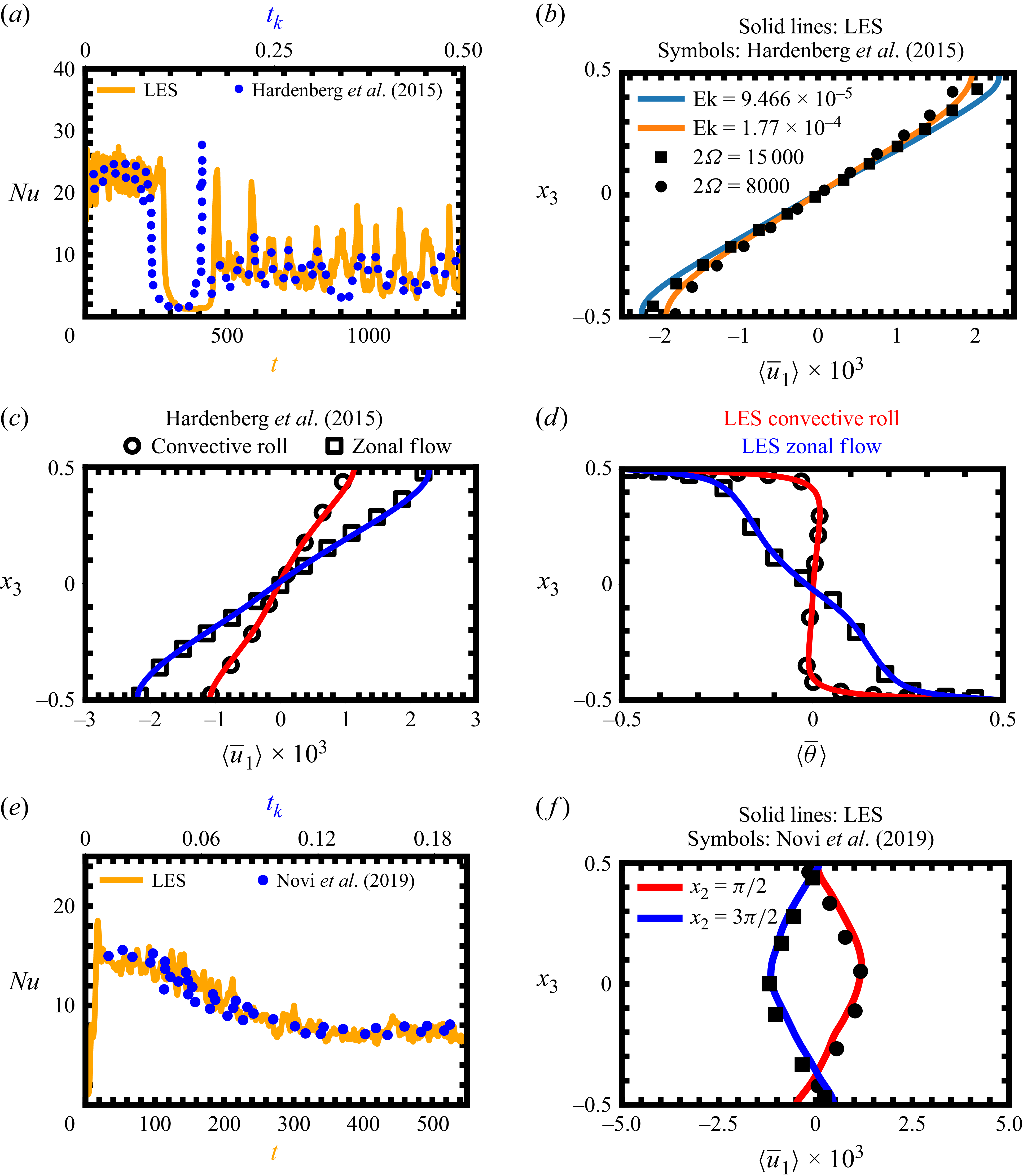
We validate our LES solver against the DNS of Von Hardenberg et al. (Reference Von Hardenberg, Goluskin, Provenzale and Spiegel2015) for horizontal rotation and with the DNS of Novi et al. (Reference Novi, von, Jost, David, Provenzale and Spiegel2019) where the axis of rotation is tilted at an angle of
 $15^{\circ }$
from the horizontal. We perform validation for parameters
 $Ra=$
 $10^7$
,
 $\textit{Pr}= 0.71$
and
 $Ek= 1.77 \times 10^{-4},\ 1.42 \times 10^{-4},\ 9.466 \times 10^{-5}$
. These cases correspond to the dimensionless rotation rates 8000, 10 000, 15 000 cases of Von Hardenberg et al. (Reference Von Hardenberg, Goluskin, Provenzale and Spiegel2015). Time
 $t_{\kappa }$
is the non-dimensional time as per Von Hardenberg et al. (Reference Von Hardenberg, Goluskin, Provenzale and Spiegel2015) and
 $t$
is the non-dimensional time of the present study. The flow transitions from convective roll to zonal flow near
 $t_{\kappa } = 0.08$
. Von Hardenberg et al. (Reference Von Hardenberg, Goluskin, Provenzale and Spiegel2015) report
 $\textit{Nu} = 22.6$
for the convective roll and
 $\textit{Nu} = 7.1$
for the zonal flow. We obtain
 $\textit{Nu} = 22.556$
for the convective roll and
 $\textit{Nu} = 7.529$
for the zonal flow. We plot the time-averaged
 $\langle \overline {u}_1 \rangle$
profiles for different rotation rates in figure 2(b). The change in the time-averaged horizontal velocity
 $\langle \overline {u}_1 \rangle$
and
 $\langle \overline {\theta } \rangle$
as flow transitions from convective roll to zonal flow is depicted in figures 2(c) and 2(d), respectively. We compare the time evolution of
 $\textit{Nu}$
(figure 2
e) and the time-averaged vertical profile of
 $\langle \overline {u}_{1} \rangle$
(figure 2
f) for the tilted axis (
 $15^{\circ }$
) of rotation obtained from our LES with the results of Novi et al. (Reference Novi, von, Jost, David, Provenzale and Spiegel2019). Our LES results are in very good agreement with the results of Von Hardenberg et al. (Reference Von Hardenberg, Goluskin, Provenzale and Spiegel2015) and Novi et al. (Reference Novi, von, Jost, David, Provenzale and Spiegel2019). Further validation of the present LES solver in comparison with DNS of Guervilly & Hughes (Reference Guervilly and Hughes2017) for vertically RRBC is presented in Appendix B.
Validation of LES solver with (a–d) Von Hardenberg et al. (Reference Von Hardenberg, Goluskin, Provenzale and Spiegel2015) (
 $2\varOmega (Ek) = 8000 (1.77\times 10^{-4})$
,
 $10\,000 (1.42\times 10^{-4})$
,
 $15\,000 (9.468 \times 10^{-5})$
) and (e, f) Novi et al. (Reference Novi, von, Jost, David, Provenzale and Spiegel2019), where
 $Ra = 10^7$
for all the plots. (a) The
 $\textit{Nu}$
time series, (b) time-averaged horizontal velocity
 $\langle \overline {u}_1 \rangle$
along the vertical for different rotation rates, transition in time-averaged vertical profiles of (c)
 $\langle \overline {u}_1 \rangle$
and (d)
 $\langle \overline {\theta } \rangle$
, (e)
 $\textit{Nu}$
time series and ( f) time-averaged
 $\langle \overline {u}_1 \rangle$
for the rotational axis tilted at an angle of
 $15^\circ$
.

Table 1 lists all the simulation cases, the parameter regime and the corresponding grid size in the respective directions. The size of the domain is
 $2\pi \times 2\pi \times 1$
with the boundary conditions (2.6) for velocity and (2.7) for temperature.
3. Results
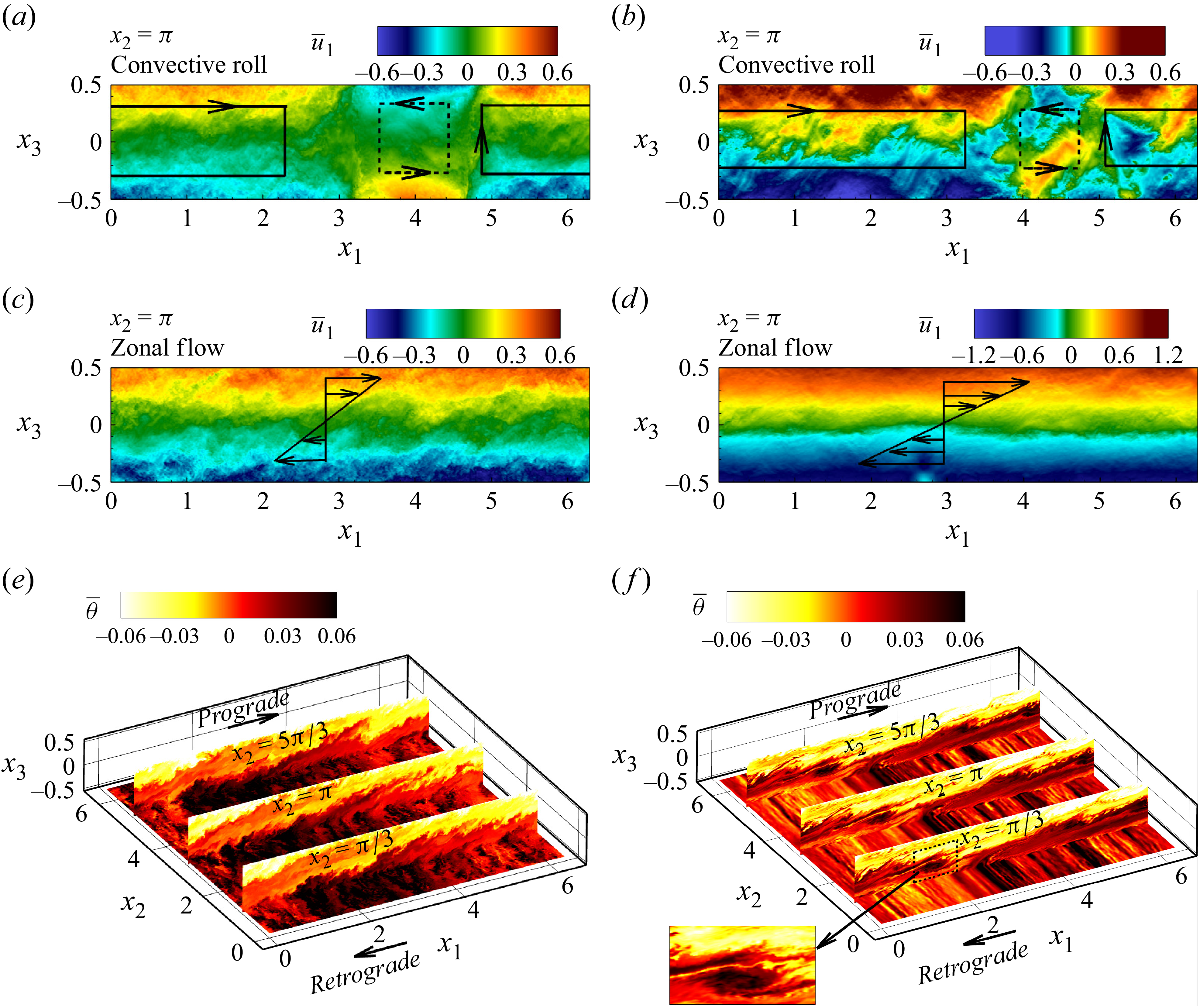
We demonstrate the convective roll phase for
 $Ra=$
 $10^{12}$
with
 $Ek=$
 $10^{-6}$
(figure 3
a) and
 $Ek=$
 $10^{-7}$
(figure 3
b). These convective rolls are characterised by a widening cyclonic roll and a narrowing anti-cyclonic roll (Von Hardenberg et al. Reference Von Hardenberg, Goluskin, Provenzale and Spiegel2015). The zonal flow state is initiated when the anti-cyclonic roll completely disappears. Figures 3(c) for Ra12E6 and 3(d) for Ra12E7 show the zonal flow has
 $\overline {u}_{1} \gt 0$
near the top plate and
 $\overline {u}_{1} \lt 0$
near the bottom plate and is vertically sheared. The impact of this shear is visible on the thermal plumes as shown using the
 $\overline {\theta }$
contours at the vertical planes
 $x_{2}$
=
 $\pi$
/3,
 $\pi$
and 5
 $\pi$
/3 in figure 3(e) for
 $Ra12E6$
and figure 3( f) for
 $Ra12E7$
. The hot plumes near the bottom plate are sheared by the retrograde (
 $-x_{1}$
)-moving wind and the prograde (
 $+$
 $x_{1}$
)-moving wind shears the cold plumes near the top plate thus establishing a large-scale vertically sheared flow with significant mean in the horizontal direction (see supplementary movies S1, S2, S3 and S4 available at https://doi.org/10.1017/jfm.2026.11479). We observe similar flow evolution for
 $Ra = 10^{12},\ Ek = 10^{-8}$
(see supplementary movies S5 and S6).
The cases corresponding to different
 ${\textit{Ra}}$
and
 ${\textit{Ek}}$
. The domain lengths in
 $x_{1}$
,
 $x_{2}$
and
 $x_{3}$
are
 $2\pi$
,
 $2\pi$
and 1, respectively.

Instantaneous flow visualisation for the cases
 $Ra=$
 $10^{12}$
and
 $Ek=$
 $10^{-6}$
(a,c) and
 $Ra=$
 $10^{12}$
and
 $Ek=$
 $10^{-7}$
(b,d) for convective roll (a,b) and zonal flow (c,d) state. (e, f) The temperature contours in the zonal flow state.

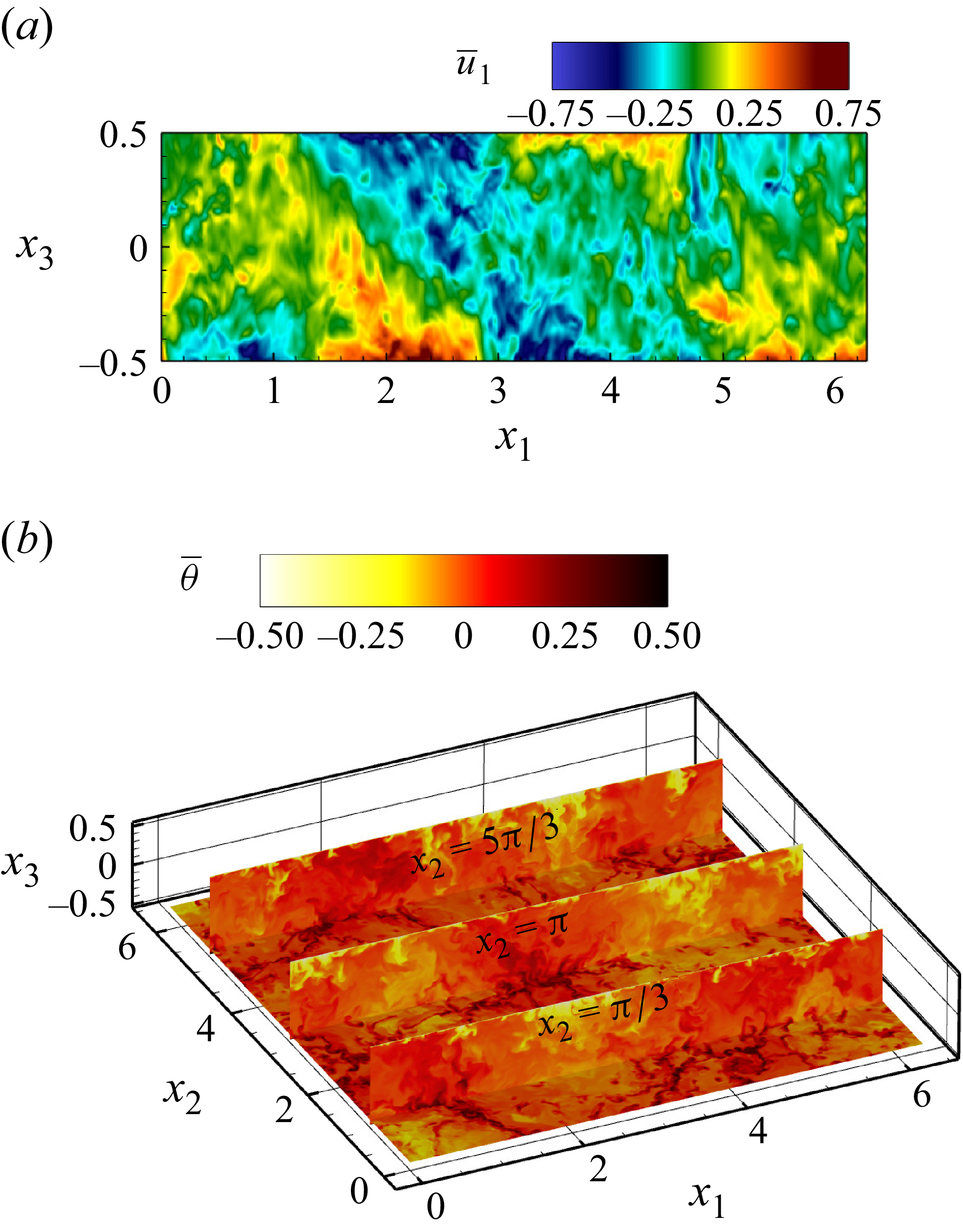
Instantaneous visualisation of
 $Ra8E3$
. (a) The velocity field
 $\overline {u}_1$
and (b) temperature contour
 $\overline {\theta }$
.

We also show the flow field for the
 $Ra8E3$
case in figure 4. The
 $\overline {u_1}$
contours in figure 4(a) demonstrate the disintegration of the weak convective rolls. Similarly, the thermal plumes (figure 4
b) emanate from the respective boundaries but remain unsheared owing to the weak and disintegrated convective rolls.
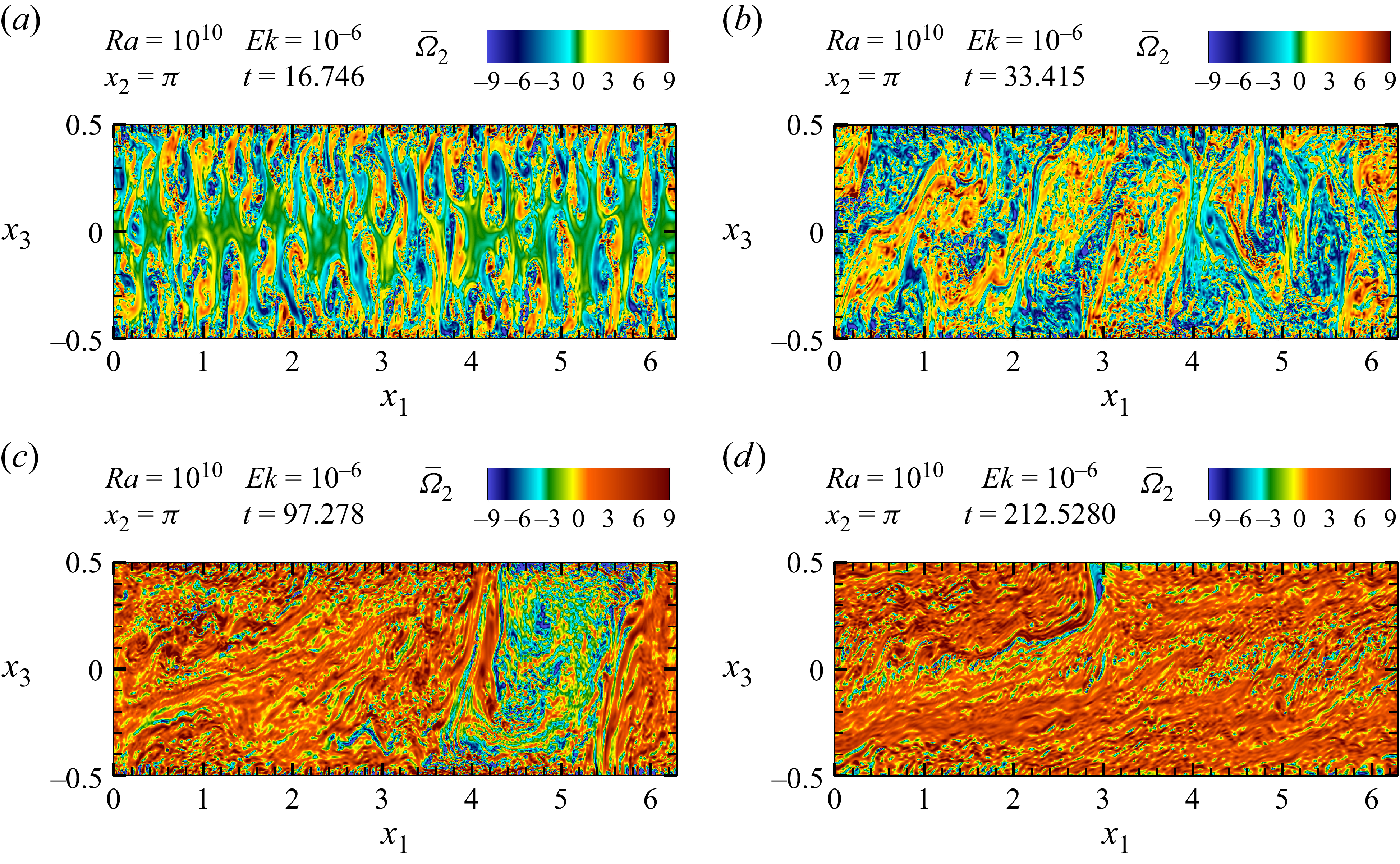
The vorticity plots for
 $Ra10E6$
at
 $t=$
(a) 16.746, (b) 33.415, (c) 97.278 and (d) 212.528.

Under the influence of rapid rotation, RBC demonstrates vortex-merging events where small vortices merge to form large vortices at a size comparable to the size of the domain (Rubio et al. Reference Rubio, Julien, Knobloch and Weiss2014; Favier et al. Reference Favier, Silvers and Proctor2014). We demonstrate the same process for the case
 $Ra10E6$
in figure 5. On the onset at
 $t = 16.746$
, as shown in figure 5(a), both cyclonic and anti-cyclonic vortices emerge. The vortex merging begins, and vortices grow in size (
 $t = 33.415$
; figure 5
b). As the mean flow strengthens, the cyclonic vortex strengthens, as shown in figure 5(c) at
 $t = 97.278$
. This process continues until the entire domain consists of a cyclonic vortex in the zonal flow phase as indicated in figure 5(d) at
 $t = 212.5280$
. Such large-scale shear with horizontal mean component has been studied in a two-dimensional RBC set-up by Goluskin (Reference Goluskin2013), Goluskin et al. (Reference Goluskin, Johnston, Flierl and Spiegel2014), Fitzgerald & Farrell (Reference Fitzgerald and Farrell2014) and Liu et al. (Reference Liu, Sharma, Julien and Knobloch2024). However, the strength and cause of this mean flow in three-dimensional horizontally RRBC in the
 $Ra{-}Ek$
parameter space remain unexplored (Von Hardenberg et al. Reference Von Hardenberg, Goluskin, Provenzale and Spiegel2015; Wang et al. Reference Wang, Chong, Stevens, Verzicco and Lohse2020).
Time-averaged mean profiles of (a)
 $\langle \overline {u}_{1} \rangle$
and (b)
 $\langle \overline {\theta } \rangle$
for the cases corresponding to
 $ {1}/{Ro_c}=$
 $16.852$
.

3.1. Mean profiles
To understand the mean flow characteristics, we plot the time-averaged streamwise mean velocity
 $\langle \overline {u}_{1} \rangle$
and the time-averaged mean non-dimensional temperature
 $\langle \overline {\theta } \rangle$
in figures 6(a) and 6(b), respectively, after zonal flow forms for cases at
 $1/Ro_c = 16.852$
. The velocity profile (figure 6
a) becomes increasingly linear as
 ${\textit{Ra}}$
is increased at
 $1/Ro_c =$
 $16.852$
. However, the shear stress at the plates vanishes due to the imposed stress-free boundary condition. The linearity spreads further towards the plates as
 ${\textit{Ra}}$
increases to
 $10^{12}$
. This is indicative of the development of a strong mean velocity field with an increase in
 ${\textit{Ra}}$
.
The mean temperature profile in figure 6(b) also changes significantly with increasing
 ${\textit{Ra}}$
. The
 $Ra8E5$
temperature profile is linear, implying that heat is transported solely due to diffusion. This linear mean temperature profile is altered when
 ${\textit{Ra}}$
increases for
 $Ra9E6$
,
 $Ra10E6$
,
 $Ra11E7$
and
 $Ra12E7$
. The departure from the linear mean temperature profile signifies heat transfer owing to convection instead of diffusion. Near the plates, steep thermal boundary layers begin to develop, followed by a near-wall region with significant convection; however, the interior remains linear. When
 ${\textit{Ra}}$
is further increased for
 $Ra12E7$
, convection becomes even more significant, and the thermal boundary layer becomes steeper compared with the other cases.The unstable linear stratification in the interior is altered significantly for
 $Ra12E7$
, where the temperature profile approaches isothermal behaviour.
Time evolution of
 $\textit{Re}_{\mathcal{M}}$
and
 $\textit{Re}_{\mathcal{K}}$
(semilog y axis) for cases (a)
 $Ra8E5$
, (b)
 $Ra10E5$
, (c)
 $Ra10E6$
, (d)
 $Ra10E7$
, (e)
 $Ra12E7$
and ( f)
 $Ra12E8$
.

3.2. Reynolds number and energy transfer between mean and turbulence
To quantify the strength of mean shear, we define the mean kinetic energy in terms of the Reynolds number
 $\textit{Re}_{\mathcal{M}}$
(3.1a
). As we demonstrate that this mean emerges at the expense of TKE, we also define
 $\textit{Re}_{\mathcal{K}}$
(3.1b
). Mathematically,
 $\textit{Re}_{\mathcal{M}}$
and
 $\textit{Re}_{\mathcal{K}}$
are calculated as follows:
 \begin{align} \textit{Re}_{\mathcal{M}}= \sqrt {\frac {Ra}{\textit{Pr}}\langle \overline {u_{i}}\rangle \hspace {0.1cm} \langle \overline {u_{i}}\rangle } , \quad \textit{Re}_{\mathcal{K}}= \sqrt {\frac {Ra}{\textit{Pr}}\langle \overline {u_{i}}^{\prime }\hspace {0.1cm} \overline {u_{i}}^{\prime }}\rangle . \end{align}
Figure 7 shows the time evolution of
 $\textit{Re}_{\mathcal{M}}$
and
 $\textit{Re}_{\mathcal{K}}$
(semilog y axis) for different
 ${\textit{Ra}}$
and
 ${\textit{Ek}}$
combinations. In figure 7(a) for the case
 $Ra8E5$
(
 $Ra = 10^{8}$
and
 $Ek = 10^{-5}$
), we can observe that
 $\textit{Re}_{\mathcal{M}} \lt \textit{Re}_{\mathcal{K}}$
for a certain period indicating that the turbulent field is stronger than the mean field. This duration when
 $\textit{Re}_{\mathcal{M}} \lt$
 $\textit{Re}_{\mathcal{K}}$
is the convective roll phase. When
 $\textit{Re}_{\mathcal{M}}$
overtakes
 $\textit{Re}_{\mathcal{K}}$
, the convective rolls merge to form zonal flow, and the mean field becomes stronger than the turbulent field. We can also observe a decrease in
 $\textit{Re}_{\mathcal{K}}$
signifying energy transfer to the mean flow. We observe a similar evolution of
 $\textit{Re}_{\mathcal{M}}$
and
 $\textit{Re}_{\mathcal{K}}$
for
 $Ra = 10^{10}, Ek = 10^{-5}$
,
 $Ra = 10^{10}, Ek = 10^{-6}$
,
 $Ra = 10^{10}, Ek = 10^{-7}$
,
 $Ra = 10^{12}, Ek = 10^{-7}$
and
 $Ra = 10^{12}, Ek = 10^{-8}$
in figures 7(b)–7( f), respectively. The insets of figure 7 show the continuous accumulation of kinetic energy in the mean field.
To further enhance our understanding of how this exchange between mean and turbulence is facilitated, we analyse the TKE budget terms given as follows:
 \begin{equation} \frac {{\rm d} \mathcal{K}}{{\rm d}t} = \mathcal{P} + \mathcal{B} - \varepsilon - \varepsilon _{\textit{sgs}} - \frac {\partial \Im _{i}}{\partial x_{i}} -\frac {\partial \Im _{i,sgs}}{\partial x_{i}}, \end{equation}
where
 \begin{equation} \mathcal{K}=\frac {1}{2} \big \langle \overline {u_{i}}^{\prime }\overline {u_{i}}^{\prime } \big \rangle \end{equation}
is the TKE and
 \begin{align} \mathcal{P} = - \big \langle \overline {u}_{i}^{\prime }\hspace {0.1cm}\overline {u}^{\prime}_{\!j} \big \rangle \frac {{\rm d}\langle \overline {u}_{i} \rangle }{{\rm d}x_{\!j}}, \quad \mathcal{B} = \big \langle \overline {u}_{3}^{\prime } \hspace {0.1cm} \overline {\theta }^{\prime } \big \rangle \end{align}
represent the turbulent production and buoyancy flux, respectively, and
 \begin{equation} \varepsilon =2\sqrt {\frac {\textit{Pr}}{Ra}} \big \langle \overline {s}_{ij}^{\prime } \hspace {0.1cm} \overline {s}_{ij}^{\prime } \big \rangle , \end{equation}
where
 $s_{ij}^{\prime } = ({1}/{2}) ( {\partial u_i^{\prime }}/{\partial x_j} + {\partial u^{\prime}_j}/{\partial x_i} )$
is the turbulent dissipation rate. The transport term
 $ {\partial \Im _{i}}/{\partial x_{i}}$
is defined with
 \begin{equation} \Im _{i} = \frac {1}{2} \big \langle \overline {u}_{i}^{\prime } \hspace {0.1cm} \overline {u}_{\!j}^{\prime } \hspace {0.1cm}\overline {u_{\!j}^{\prime }} \big \rangle +\langle \overline {u}_{i}^{\prime } \hspace {0.1cm} \overline {p}^{\prime } \rangle - 2\sqrt {\frac {\textit{Pr}}{Ra}} \big \langle \overline {u}_{\!j}^{\prime } \hspace {0.1cm} \overline {S}_{ij}^{\prime } \big \rangle . \end{equation}
The subgrid dissipation
 $\varepsilon _{\textit{sgs}}$
is defined as
 \begin{equation} \varepsilon _{\textit{sgs}} = - \Bigg \langle \tau _{ij}^{\prime } \frac {\partial \overline {u_{i}}^{\prime }}{\partial x_{\!j}} \Bigg \rangle , \end{equation}
whereas the subgrid transport
 $ {\partial \Im _{i,sgs}}/{\partial x_{i}}$
is defined with
 \begin{equation} \Im _{i,sgs} = \big \langle \tau _{ij}^{\prime }\overline {u_{i}}^{\prime } \big \rangle . \end{equation}
Time evolution (a,c,e,g) and time-averaged vertical variation (b,d, f,h) of TKE budgets for
 $Ra8E3$
(a,b),
 $Ra10E5$
(c,d),
 $Ra12E7$
(e, f) and
 $Ra12E8$
(g,h).

The TKE budget equation signifies energy conservation. Zonal flow does not form for
 $Ra7E3$
,
 $Ra8E3$
and
 $Ra9E4$
(
 $1/Ro_c=$
 $0.16852$
) and the main balance remains between
 $\mathcal{B}$
and
 $\varepsilon$
,
 $\varepsilon _{\textit{sgs}}$
as shown in figure 8(a) for
 $Ra8E3$
. Similar plots for
 $Ra7E3$
and
 $Ra9E4$
are shown in figures 16(a) and 16(c), respectively, in Appendix C. We see that for the case
 $Ra10E5$
(
 $Ra=$
 $10^{10}$
and
 $Ek=$
 $10^{-5}$
) in figure 8(c), during the convective roll phase the buoyancy flux (
 $\mathcal{B}$
) converts the potential energy to TKE. At this instant, a portion of this TKE is transferred to the mean field as shown by the negative production term while the remaining TKE dissipates owing to
 $\varepsilon _{\textit{sgs}}$
and
 $\varepsilon$
. Here
 $\mathcal{P} \gt 0$
represents extraction and energy transfer from the mean to turbulence. In contrast,
 $\mathcal{P} \lt 0$
indicates energy transfer from small-scale turbulence to the mean fields (Kundu, Cohen & Dowling Reference Kundu, Cohen and Dowling2015). When
 $\textit{Re}_{\mathcal{M}}$
overtakes
 $\textit{Re}_{\mathcal{K}}$
in figure 7(b), we find a sudden drop in
 $\mathcal{P}$
to negative values, implying energy draining from turbulence to the mean. The flow transitions at this instant from the convective roll phase to zonal flow (see supplementary movies S7 and S8). The transfer to the mean becomes significant in the cases
 $Ra12E7$
(figure 8
e) and
 $Ra12E8$
(figure 8
g). Note that we only plot the TKE budget after the zonal flow forms for the cases
 $Ra12E7$
and
 $Ra12E8$
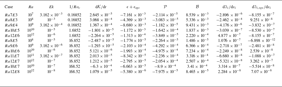
. The balance is defined as the sum of the terms on the right-hand side of (3.2). The transport and the subgrid transport terms remain significantly smaller than the rest of the terms (table 2), and therefore are not shown in the line plots. We achieve close agreement between the unsteady term and balance for all our cases. Thus, our grid spacing is sufficient to resolve the relevant scales of motion (Pal & Chalamalla Reference Pal and Chalamalla2020).
The cases corresponding to different
 ${\textit{Ra}}$
and
 ${\textit{Ek}}$
. The domain lengths in
 $x_1$
,
 $x_2$
and
 $x_3$
are
 $2\pi$
,
 $2\pi$
and 1, respectively.

We plot the time-averaged TKE budget terms along the vertical for
 $Ra8E3$
as shown in figure 8(b) (see figures 16
b and 16
d for
 $Ra7E3$
and
 $Ra9E4$
, respectively, in Appendix C), and find that the primary balance is among
 $\mathcal{B}$
,
 $\varepsilon$
and
 $\varepsilon _{\textit{sgs}}$
, with
 $\mathcal{P}$
 $\sim 0$
. Figures 8(d), 8( f) and 8(h) show the time-averaged vertical variation of the TKE budget terms in the zonal flow phase for different cases. For
 $Ra10E5$
we can notice a lower
 $\mathcal{P}$
compared with
 $\varepsilon _{\textit{sgs}}$
and
 $\varepsilon$
. The energy released by
 $\mathcal{B}$
in the domain is mostly dissipated, and the remaining fraction transfers to the mean. However,
 $\mathcal{P}$
becomes significantly negative for the cases
 $Ra12E7$
(figure 8
f) and
 $Ra12E8$
(figure 8
h), indicating energy transfer from turbulence to the mean field, with a relatively smaller portion being dissipated.
We present the time-averaged vertically integrated TKE budget terms for all the simulations in table 2. In the non-zonal flow cases
 $Ra7E3$
,
 $Ra8E3$
and
 $Ra9E4$
we observe the main balance between
 $\mathcal{B}$
and
 $\varepsilon +\varepsilon _{\textit{sgs}}$
. However, for the rest of the cases where zonal flow forms (time-averaging performed in the zonal flow phase only), the primary balance is among
 $\mathcal{B}$
,
 $\mathcal{P}$
and
 $\varepsilon +\varepsilon _{\textit{sgs}}$
. In the zonal flow cases, for
 $1/Ro_c=$
 $1.6852$
we observe leading-order balance between
 $\mathcal{B}$
and
 $\varepsilon +\varepsilon _{\textit{sgs}}$
with
 $\mathcal{P}$
in the subleading order. The effect of rotation in comparison with thermal forcing increases for the cases with
 $1/Ro_c=$
 $16.852$
wherein we observe
 $\varepsilon +\epsilon _{\textit{sgs}}$
decreases in magnitude and balance between
 $\mathcal{B}$
and
 $\mathcal{P}$
takes the leading order as we move from
 $Ra8E5$
towards
 $Ra12E7$
. Similar decrease in
 $\varepsilon +\varepsilon _{\textit{sgs}}$
can be observed for
 $Ra10E7$
and
 $Ra12E8$
, where the effect of rotation dominates thermal forcing for the cases with
 $1/Ro_c=$
 $168.52$
. The time-averaged vertically integrated TKE budgets hence distinguish the flow in horizontally RRBC based on the relative impact of rotation and thermal forcing.
In many turbulent flows, an imposed anisotropic mean field facilitates turbulent production (Pham & Sarkar Reference Pham and Sarkar2014a
,
Reference Pham and Sarkarb
; Olsthoorn, Kaminski & Robb Reference Olsthoorn, Kaminski and Robb2023). However, in the present scenario, the mean anisotropy naturally develops from the underlying buoyant small-scale turbulence due to horizontal rotation. Recently Wang et al. (Reference Wang, Wang, Wan and Sun2021) studied the TKE budget for convective rolls and zonal flow phase in a three-dimensional RBC set-up without rotation. Initialising the simulations with linear shear-flow velocity initial conditions, they reported a balance between
 $\mathcal{B}$
and
 $\varepsilon$
for the zonal flow phase and between
 $\mathcal{P}$
and
 $\varepsilon$
for the convective roll phase. The simulations reported in this work were initialised from rest. We found that
 $\mathcal{B}$
is the source of turbulence during both convective roll and zonal flow in contrast to the findings of Wang et al. (Reference Wang, Wang, Wan and Sun2021). Further, with the increase in
 $1/Ro$
,
 $\mathcal{P}$
becomes prominent in the TKE budget balance and is the primary agency transferring energy to the mean flow.
The total kinetic energy spectra plots for
 $Ra=$
 $10^{12}$
,
 $Ek=$
 $10^{-6}$
(a,d,g),
 $Ra=$
 $10^{12}$
,
 $Ek=$
 $10^{-7}$
(b,e,h) and
 $Ra=$
 $10^{12}$
,
 $Ek=$
 $10^{-8}$
(c, f,i). (a–f) Spectra at instances when zonal flow has already been established. (g–i) Comparison of the spectra at the convective roll phase and the zonal flow state.

3.3. Energy spectra and inverse energy cascade
We plot the total kinetic energy spectra in figure 9 to further corroborate the energy transfer from small scales to the mean field. The kinetic energy distribution across scales is due to nonlinear interactions. The energy amongst the scales is quantified by the Fourier transform of the velocity field, denoted as
 $\widehat {u_{i}}(\boldsymbol {k})$
. Here,
 $\boldsymbol {k} = (k_{x_1}$
,
 $k_{x_2}$
) is the wave vector in Fourier space and
 $\lvert \boldsymbol {k} \rvert ^{-1}$
is proportional to the scale of motion. For a thin ring of radius
 $k = \lvert \boldsymbol {k} \rvert$
on the horizontal plane, the total kinetic energy spectrum function is defined as
 \begin{equation} E_{t}(k) = \oint \frac {1}{2}\varPhi _{ii}(\boldsymbol {k}) \, {\rm d}\mathcal{C}(k) = E_{11} + E_{22} + E_{33}, \end{equation}
where
 $\varPhi _{ii}(\boldsymbol {k})$
represents the trace of the velocity spectrum given in general tensor form as
 $\varPhi _{ij}(k)=$
 $\widehat {u}_{i}^{*}(k)$
 $\widehat {u}_{\!j}(k)$
. The term
 $\oint () \, {\rm d}\mathcal{C}(k)$
denotes integration over the circumference of the ring of radius
 $k$
, while
 $E_{11},$
 $E_{22}$
and
 $E_{33}$
are the directional components of
 $E_{t}$
. Numerically, we obtain the normalised Fourier-transformed velocity fields
 $\widehat {u_{1}},$
 $\widehat {u_{2}}$
and
 $\widehat {u_{3}}$
in the wave vector domain
 $(k_{x_1},k_{x_2})$
on different horizontal planes. The diagonal components
 $\varPhi _{11}$
,
 $\varPhi _{22}$
and
 $\varPhi _{33}$
of the velocity spectrum tensor are calculated, and the zero frequency component is shifted to the centre of the domain. The total energy stored in each integral radial bin (
 $k=$
 $\sqrt {k_{x_1}^2 + k_{x_2}^2}$
rounded to the nearest integer) is then calculated to obtain the energy spectra.
In figure 9 the left-hand column shows spectra plots for
 $Ra = 10^{12}$
,
 $Ek = 10^{-6}$
, the middle column for
 $Ra = 10^{12}$
,
 $Ek = 10^{-7}$
and the right-hand column for
 $Ra = 10^{12}$
,
 $Ek = 10^{-8}$
. These plots provide an estimate of energy distribution across different scales of motion. For different parameters (figure 9
a–c), we find a sudden jump in the energy spectra at large wavenumbers. The magnitude of this sudden jump decreases as we move up vertically from
 $x_{3}=$
 $-0.435$
(near the wall) towards
 $x_{3}=$
 $-0.0029$
(middle of the domain). Several studies have investigated the effect of forcing and subsequent cascade of energy in two-dimensional turbulence (Yakhot Reference Yakhot1999; Boffetta & Ecke Reference Boffetta and Ecke2012; Poujol et al. Reference Poujol, van Kan and Alexakis2020; Sofiadis, Sarris & Alexakis Reference Sofiadis, Sarris and Alexakis2023) and, more recently, in three-dimensional turbulence (Alexakis et al. Reference Alexakis, Marino, Mininni, van Kan, Foldes and Feraco2024; de Wit et al. Reference de Wit, Fruchart, Khain, Toschi and Vitelli2024). Unlike the literature, the forcing is natural in our cases due to the momentum equation’s buoyancy term. For
 $1/Ro_c = 1.68522$
,
 $16.852$
and
 $168.52$
, the energy deposited at small scales owing to the work done by buoyancy transfers to large scales via nonlinear interactions and forms zonal flow Goluskin (Reference Goluskin2013). The source of the thermal forcing is the thermal plumes that lose coherence while proceeding from
 $x_{3}=-0.435$
to
 $x_{3}=-0.0029$
, owing to dispersion caused by the sheared velocity field. Figure 9(d–f) shows the contribution to
 $E_{t}(k)$
from the components
 $E_{11}$
,
 $E_{22}$
and
 $E_{33}$
. The forcing is predominantly in the
 $E_{33}$
spectra rather than
 $E_{11}$
. Note that
 $E_{11}$
stays at least two orders of magnitude above
 $E_{33}$
or
 $E_{22}$
at large scales. The buoyancy forces the components along gravity, from where the anisotropic effect of rotation causes it to transfer to the zonally extended component
 $E_{11}$
via nonlinear interactions (Goluskin Reference Goluskin2013; Von Hardenberg et al. Reference Von Hardenberg, Goluskin, Provenzale and Spiegel2015). Further, figure 9(g–i) shows that energy in the zonal flow state is greater than in the convective roll phase at large scales. It can also be observed from the right-hand column in figure 9 that the extent of forcing at small scales increases with an increase in rotation. Therefore, we conclude that rotation significantly influences the transfer of energy to
 $E_{11}$
.
The energy flux versus
 $k_{x_1}$
for
 $ {1}/{Ro_C}=$
(a) 0.16852, (b) 1.6852, (c) 16.852 and (d) 168.52. Horizontal dashed lines,
 $\varPi = 0$
; vertical dashed lines,
 $k_{x_1} = 10$
.

The advection term in the momentum equation is responsible for the energy transfer across different scales of motion. The upscale energy transfer in zonal flows has been suggested earlier (Heimpel et al. Reference Heimpel, Aurnou and Wicht2005; Goluskin Reference Goluskin2013) but has never been proved for zonal flows. Therefore, we compute the energy flux
 $\varPi (k_{x_1})$
in figure 10 to demonstrate the upscale energy transfer. Following Frisch (Reference Frisch1995) and Alexakis & Biferale (Reference Alexakis and Biferale2018), we define the spectral energy flux along the horizontal wave modes
 $k_{x_1}$
as
 \begin{equation} \varPi (k_{x_1},x_3) = \left \langle \overline {u_i}^{\lt k_{x_1}} \overline {u_j}\frac {\partial \overline {u_i}}{\partial x_j} \right \rangle , \end{equation}
where
 $\overline {u_i}^{\lt k_{x_1}}$
is given as
 \begin{equation} \overline {u}_{i}^{\lt k_{x_1}}(\boldsymbol{x})= \sum _{\lvert K_{x_1} \rvert \lt k_{x_1}} \hat {u_{i}}(\boldsymbol{K}) e^{\iota {\boldsymbol{K} \boldsymbol{\cdot }\boldsymbol{x}}}, \end{equation}
with
 $\boldsymbol{K}=$
 $(K_{x_1},K_{x_2})$
being the wave vector in spectral space. This is termed spectral filtering (Frisch Reference Frisch1995; Alexakis & Biferale Reference Alexakis and Biferale2018) where Fourier modes that satisfy the condition
 $\lvert K_{x_1} \rvert \lt k_{x_1}$
are kept and all other modes are set to zero. Further, the spatial average
 $\langle \cdots\rangle$
in two dimensions is mathematically the same as (2.19). Flux
 $\varPi (k_{x_1},x_3)$
is the flux evaluated on different horizontal planes. The velocity
 $\overline {u}_{i}$
and the advection term
 $\overline {u}_{\!j}$
 $\partial \overline {u}_{i}$
/
 $\partial x_{\!j}$
are calculated at the cell centre. Due to periodic boundary conditions in the horizontal plane, we restrict ourselves to calculating only the terms
 $\overline {u}_{1}\overline {u}_{3}$
 $\partial \overline {u}_{1}$
/
 $\partial x_{3}$
and
 $\overline {u}_{2}\overline {u}_{3}$
 $\partial \overline {u}_{2}$
/
 $\partial x_{3}$
. These terms physically represent vertical advection of horizontal kinetic energy. Turbulence in the presence of zonal flow is anisotropic with strong vertically sheared mean flow in the horizontal direction (
 $+x_{1}$
). Hence, we use the total velocity fields (including mean and fluctuations) to perform mode-by-mode analysis by employing the filter defined in (3.11) that filters modes in the horizontal direction or the direction of zonal flow and expresses
 $\varPi$
in terms of
 $k_{x_1}$
. We further define integrated energy flux as
 \begin{equation} \varPi (k_{x_1}) = \frac {1}{L_{x_3}} \int _{-L_{x_3 /2}}^{+L_{x_3 /2}} \varPi (k_{x_1},x_3) {\rm d}x_3. \end{equation}
Intuitively,
 $\varPi (k_{x_1})$
could be understood as the counterpart of
 $\mathcal{P}$
in the wavenumber domain. Here
 $\varPi (k_{x_1}) \gt 0$
implies the transfer of energy to small scales (forward cascade), and the energy moves towards large scales when
 $\varPi (k_{x_1}) \lt 0$
(inverse cascade) (Alexakis & Biferale Reference Alexakis and Biferale2018). We plot
 $\varPi (k_{x_1})$
for different cases in figure 10. The non-zonal flow cases
 $Ra7E3$
,
 $Ra8E3$
and
 $Ra9E4$
(
 $1/Ro_c = 0.16852$
) remain invariably positive for the entire range of
 $k_{x_1}$
, implying energy transfer to small scales. For the zonal flow cases
 $1/Ro_c = 1.6852$
,
 $16.852$
and
 $168.52$
(figures 10
b–10
d, respectively)
 $\varPi (k_{x_1})$
decreases continuously and becomes invariably negative for large scales (
 $k_{x_1} \lt 10$
). This is more pronounced for cases with
 $1/Ro_c = 16.852$
(figure 10
c) and
 $168.52$
(figure 10
d), where stronger rotation is capable of energising the large scale to a greater extent. Further,
 $\varPi (k_{x_1}) \lt 0$
at large scales leads to an increase in the mean kinetic energy, which is also supported by the plots in the insets of figure 7.
Inverse cascade is generally associated with two-dimensional flow (Frisch Reference Frisch1995). Three-dimensional flow, like that for case
 $Ra8E3$
(
 $1/Ro_c=$
 $0.16852$
; figure 10
a), typically shows a forward cascade in which energy is transferred from large to small scales, where it is eventually dissipated. As
 $1/Ro$
increases, the flow becomes increasingly two-dimensional (Favier et al. Reference Favier, Silvers and Proctor2014), and the inverse cascade begins to operate at a large scale. The importance of rapid rotation and the impact on the upscale energy transfer under the RBC set-up have been explored by Rubio et al. (Reference Rubio, Julien, Knobloch and Weiss2014), Favier et al. (Reference Favier, Silvers and Proctor2014) and Guervilly et al. (Reference Guervilly, Hughes and Jones2014). Several studies have also discovered the transition from three- to two-dimensional flow using external forcing and excluding the effects of thermal forcing (Smith, Chasnov & Waleffe Reference Smith, Chasnov and Waleffe1996; Celani, Musacchio & Vincenzi Reference Celani, Musacchio and Vincenzi2010). However, in our case, the transition from three- to two-dimensional dynamics in horizontally RRBC results from the combined action of buoyancy, rotation and stress-free horizontal boundaries (Favier et al. Reference Favier, Silvers and Proctor2014). Zonal flow in our simulations results from vortex-merging events (see figure 5), similar to the formation of large-scale structures reported for vertically RRBC (Rubio et al. Reference Rubio, Julien, Knobloch and Weiss2014; Favier et al. Reference Favier, Silvers and Proctor2014; Guervilly et al. Reference Guervilly, Hughes and Jones2014). Our analysis differs from the investigations of Rubio et al. (Reference Rubio, Julien, Knobloch and Weiss2014), Favier et al. (Reference Favier, Silvers and Proctor2014) and Guervilly et al. (Reference Guervilly, Hughes and Jones2014) as we present a comprehensive scale-to-scale analysis in the direction of zonal flow including the mean flow. Retaining only the vertical advection term isolates the vertical advection responsible for the transfer of horizontal kinetic energy across scales. The vertically integrated flux (see (3.12)) presents the nature of energy transfer in the entire domain rather than decomposing the flow in barotropic (depth-independent) and baroclinic (depth-dependent) modes (Rubio et al. Reference Rubio, Julien, Knobloch and Weiss2014; Favier et al. Reference Favier, Silvers and Proctor2014)
3.4. Forces, fluctuating velocities and Reynolds stresses
For motion subject to quasi-geostrophic dynamics, the transformation of energy to smaller scales (high wavenumber) is most unlikely (Pedlosky Reference Pedlosky2013). Hence, it becomes important to assess the geostrophic nature of our simulations. The geophysical flows are primarily geostrophic, where a primary force balance between the Coriolis force and the pressure gradient force exists (Pedlosky Reference Pedlosky2013). In the context of the zonal flows, Heimpel et al. (Reference Heimpel, Aurnou and Wicht2005) have shown that in the spherical domain, the nature of the zonal flows is geostrophic. This geostrophic balance can be achieved easily with stress-free boundary conditions, which tend to reduce the viscous dissipation and limit it within a thin layer near the boundaries. Moreover, the stress-free boundary conditions assist in modelling the outer layers of the atmosphere where zonal flow is present. Such a geostrophic balance is inherent in the RRBC set-up (King, Stellmach & Aurnou Reference King, Stellmach and Aurnou2012). Other forces may interfere with this balance, rendering a departure from geostrophy. Guzmán et al. (Reference Guzmán, Madonia, Cheng, Ostilla-Mónico, Clercx and Kunnen2021), Yan, Tobias & Calkins (Reference Yan, Tobias and Calkins2021) and Naskar & Pal (Reference Naskar and Pal2022b ) analysed the force balance in a vertically RRBC set-up. However, the nature of different forces during the zonal flow phase in a horizontally RRBC set-up is unexplored. In the earlier discussions, we demonstrated the upscale transfer of energy from small scales to mean scales. We further want to corroborate this finding by analysing the force balance, velocity fluctuations and Reynolds stresses. Following Yan et al. (Reference Yan, Tobias and Calkins2021) and dropping the terms with a magnetic field or Lorentz force, the different forces involved in this problem set-up can be expressed as
 \begin{equation} \underbrace {\frac {\partial \overline {u}_{i}^{\prime }}{\partial t}}_{F_{I}} + \underbrace {\overline {u}_{\!j}^{\prime }\frac {\partial \overline {u}_{i}^{\prime }}{\partial x_{\!j}}}_{F_{A}} = -\underbrace {\frac {\partial \overline {p}^{\prime }}{\partial x_{i}}}_{F_{P}} + \underbrace {\frac {2}{Ek}\sqrt {\frac {\textit{Pr}}{Ra}}\epsilon _{ij2}\overline {u}_{\!j}^{\prime }}_{F_{C}} + \underbrace {\overline {\theta }^{\prime }\delta _{i3}}_{F_{B}} + \underbrace {\sqrt {\frac {\textit{Pr}}{Ra}}\frac {\partial \overline {u}_{i}^{\prime }}{\partial x_{\!j}\partial x_{\!j}}}_{F_{V}}. \end{equation}
Here
 $F_{I}$
,
 $F_{A}$
,
 $F_{P}$
,
 $F_{C}$
,
 $F_{B}$
and
 $F_{V}$
are the inertial, advective, pressure gradient, Coriolis, buoyancy and viscous forces, respectively. We plot the time-averaged vertical variation of the forces in figure 11. Forces
 $F_{I}$
and
 $F_{A}$
clearly take the leading order for
 $Ra8E3$
as shown in figure 11(a) with
 $F_{C}$
being the lowest among all the forces. Force
 $F_{C}$
exceeds
 $F_{V}$
and
 $F_{B}$
when
 $1/Ro_c = 1.6852$
as demonstrated in figure 11(b) for
 $Ra10E5$
. Geostrophy, i.e.
 $F_{C}$
 $\sim$
 $F_{P}$
, comes in the leading-order balance in the interior of the domain when the rotation rate is increased to
 $1/Ro_c =$
 $16.852$
(case
 $Ra12E7$
in figure 11
c). When the rotation is further increased to
 $1/Ro_c =$
 $168.52$
(case
 $Ra12E8$
in figure 11
d), the geostrophic balance dominates the entire domain.
Vertical variation of time-averaged forces for cases (a)
 $Ra8E3$
, (b)
 $Ra10E5$
, (c)
 $Ra12E7$
and (d)
 $Ra12E8$
.

Vertical variation of time-averaged fluctuating velocities for cases (a)
 $Ra8E3$
, (b)
 $Ra10E5$
, (c)
 $Ra12E7$
and (d)
 $Ra12E8$
.

In RBC, rotation inhibits the instabilities or fluctuations perpendicular to the plates due to the Taylor–Proudman constraint (Proudman Reference Proudman1916; Taylor Reference Taylor1923). In our simulations, horizontal rotation leads to convective rolls and zonal flow, with strong mean flow suppressing the fluctuations. The rotation for
 $Ra8E3$
is not strong enough to form a mean flow. Therefore, the velocity fluctuations dominate the flow, especially in the interior, and
 $\overline {u}_{3}$
 $^{\prime }$
contributes significantly to vertical heat transport as shown in figure 12(a). The vertical fluctuation
 $\overline {u}_{3}$
 $^{\prime }$
is reduced when
 $1/Ro_c = 1.6852$
(figure 12
b). Further,
 $\overline {u}_{1}$
 $^{\prime }$
,
 $\overline {u}_{2}$
 $^{\prime }$
and
 $\overline {u}_{3}$
 $^{\prime }$
decrease significantly when
 $1/Ro_c = 16.852$
and
 $168.52$
as manifested in figures 12(c) and 12(d), respectively.
Reynolds stresses stem from momentum transfer due to the fluctuating velocity fields (Pope Reference Pope2000). Several researchers have previously studied Reynolds stresses in a RBC set-up (Krishnamurti & Howard Reference Krishnamurti and Howard1981) and also in the context of zonal flow in spherical shells (Aurnou & Olson Reference Aurnou and Olson2001; Christensen Reference Christensen2001, Reference Christensen2002). The plumes observed in the experiments of Krishnamurti & Howard (Reference Krishnamurti and Howard1981) drifted in the horizontal direction, whereas in the spherical simulations of Aurnou & Olson (Reference Aurnou and Olson2001) and Christensen (Reference Christensen2001, Reference Christensen2002), the plumes develop a prograde tilt, thus transferring linear/angular momentum to the mean flow. We have previously established that mean flow gains strength at the expense of turbulence, and negative
 $\mathcal{P}$
transfers energy from turbulence to mean flow. Similarly, Reynolds stress contributes to momentum transfer to the mean flow. We plot the time-averaged Reynolds stress
 $\langle \overline {u}^{\prime}_{1}$
 $\overline {u}^{\prime}_{3}$
 $\rangle$
in figure 13 for
 $Ra8E3$
,
 $Ra10E5$
,
 $Ra12E7$
and
 $Ra12E8$
. We observe negative
 $\langle \overline {u}^{\prime}_{1}$
 $\overline {u}^{\prime}_{3}$
 $\rangle$
for
 $Ra8E3$
, implying momentum transfer from the walls to the velocity fluctuations via buoyancy. Therefore, the energy from thermal forcing is transferred to turbulence and eventually dissipates. The weak rotation in
 $Ra8E3$
(
 $1/Ro_c = 0.16852$
) cannot alter this momentum and energy transfer, thus preventing the development of a mean shear in the vertical direction, rendering the system inertia-dominated. In contrast, for the zonal flow cases (
 $Ra10E5$
,
 $Ra12E7$
and
 $Ra12E8$
) we observe
 $\langle \overline {u}^{\prime}_{1}$
 $\overline {u}^{\prime}_{3}$
 $\rangle \gt 0$
signifying momentum transfer from the walls to the fluctuating velocities and eventually to the mean flow. For all the cases we observe
 $\langle \overline {u}^{\prime}_{1}$
 $\overline {u}^{\prime}_{3}$
 $\rangle$
increases from the boundaries, owing to zero vertical fluctuations (
 $\overline {u}_{3}$
 $^{\prime }$
) at the walls, and reaches a maximum value near the vertical centre. Further, it is important to highlight that Reynolds stress at the centre is higher for
 $Ra10E5$
as the zonal flow has to be sustained against relatively significant viscous dissipation as compared with
 $Ra12E7$
and
 $Ra12E8$
(see figure 8
b–d).
Vertical variation of time-averaged Reynolds stress
 $\langle \overline {u}^{\prime}_{1}$
 $\overline {u}^{\prime}_{3}$
 $\rangle$
.

4. Conclusion
Large-eddy simulations are performed in three-dimensional horizontally RRBC to elucidate the origin and evolution of zonal flows. Specifically, we explore the previously unreported
 $Ra{-}Ek$
parameter space for horizontal RRBC relevant to the geophysically interesting regime. We found that LES with the dynamic Smagorinsky model captures the qualitative and quantitative features of the convective and zonal flow phases accurately when compared with the DNS results of Von Hardenberg et al. (Reference Von Hardenberg, Goluskin, Provenzale and Spiegel2015) and Novi et al. (Reference Novi, von, Jost, David, Provenzale and Spiegel2019).
Our simulations further reveal that the formation of zonal flow involves a subtle interplay between thermal forcing (
 ${\textit{Ra}}$
) and Ekman number (
 ${\textit{Ek}}$
). We obtain zonal flow when the rotational effect is comparable to or exceeds the influence of thermal forcing. We ascertain that flow remains inertia-dominated for
 $1/Ro_c = 0.16852$
and zonal flow forms for cases
 $1/Ro_c = 1.6852$
,
 $16.852$
and
 $168.52$
.
The two-dimensional simulations of Goluskin et al. (Reference Goluskin, Johnston, Flierl and Spiegel2014) report the upscale energy transfer via nonlinear interaction in zonal flows and offer several insights into the evolution of zonal flows, but their set-up lacks the influence of rotation owing to the Coriolis force. Von Hardenberg et al. (Reference Von Hardenberg, Goluskin, Provenzale and Spiegel2015) incorporated rotation in a three-dimensional set-up and observed strong zonal winds. They (Goluskin et al. Reference Goluskin, Johnston, Flierl and Spiegel2014; Von Hardenberg et al. Reference Von Hardenberg, Goluskin, Provenzale and Spiegel2015) conclude the existence of upscale energy transfer in zonal flows; however, the intricate quantitative nature remained uncertain. We provide quantitative evidence of upscale energy transfer using different parameters. The zonal flow marks the onset of large-scale shear in the streamwise velocity field
 $\overline {u}_{1}$
, dispersing the thermal plumes emanating from the respective plates. The time evolution of
 $Re$
based on the mean kinetic energy (
 $\textit{Re}_{\mathcal{M}}$
) and
 $Re$
based on the TKE (
 $\textit{Re}_{\mathcal{K}}$
) reveals that large-scale shear has a strong mean component that develops at the expense of the underlying turbulence.
To corroborate this exchange of energy, we analyse the TKE budgets. For the inertia-dominated case (
 $1/Ro_c = 0.16852$
), the work done by buoyancy (
 $\mathcal{B}$
) feeds energy to turbulence, which eventually dissipates, thus establishing a balance between buoyancy flux and dissipation
 $(\varepsilon + \varepsilon _{\textit{sgs}})$
. At
 $1/Ro_c = 1.6852$
, however, the effect of rotation becomes comparable to thermal forcing. The convective roll phase is established, which grows in size and finally merges to form zonal flows. At this point, the production (
 $\mathcal{P}$
) becomes negative, signifying energy transfer from the small-scale turbulent field to the mean flow. The dominant balance remains between
 $\mathcal{B}$
and
 $\varepsilon +\varepsilon _{\textit{sgs}}$
with
 $\mathcal{P}$
being subdominant. With an increase in rotation (
 $1/Ro_c=$
 $16.852,$
 $168.52$
), the dominant balance shifts between
 $\mathcal{B}$
and
 $\mathcal{P}$
.
We further analyse the total kinetic energy spectra and energy flux to demonstrate upscale transfer of energy in zonal flows. The total kinetic energy spectra manifest a sudden jump at large wavenumbers, signifying the work done by buoyancy. Similarly, the vertically integrated energy flux remains negative at lower wavenumbers for the zonal flow cases, indicating upscale energy transfer. Inverse cascade has previously been investigated in vertically RRBC (Rubio et al. Reference Rubio, Julien, Knobloch and Weiss2014; Favier et al. Reference Favier, Silvers and Proctor2014) by decomposing the flow into baroclinic (depth-dependent) and barotropic (depth-independent) modes. The energy supplied by the baroclinic modes transfers to the large scales in the barotropic mode. The process results in a feedback loop where large baroclinic scales take energy out of the barotropic mode, and smaller ones deposit energy back into the barotropic mode. Our methodology for reporting upscale energy transfer in terms of total kinetic energy spectra and vertically integrated energy flux is selective for systems with strong vertically sheared mean flow in the horizontal direction. The resulting flux, therefore, isolates the contribution of buoyancy-driven vertical motion to kinetic energy redistribution. External forcing in barotropic set-ups to mimic the baroclinic effects is a common practice; thus, the spectra reported in our investigation (figure 9) resemble those reported in barotropic set-ups (Sukoriansky et al. Reference Sukoriansky, Dikovskaya and Galperin2007, Reference Sukoriansky, Dikovskaya and Galperin2008). We also find that large-scale vertically sheared zonal flow forms as a result of the merging of cyclonic vortices similar to that reported by Rubio et al. (Reference Rubio, Julien, Knobloch and Weiss2014), Favier et al. (Reference Favier, Silvers and Proctor2014) and Guervilly et al. (Reference Guervilly, Hughes and Jones2014) for vertically RRBC. However, in our set-up, strong zonal flows develop without two-dimensional approximations.
Although we have proved that the kinetic energy deposited at small scales by buoyancy work is carried upscale via nonlinear interactions, the intricate nature of these interactions among the individual scales will be assessed in future work. Recently, Böning et al. (Reference Böning, Wulff, Dietrich, Wicht and Christensen2023) reported that upscale energy transfer is directly driven by Reynolds stress in spherical (bounded) geometry. However, Böning et al. (Reference Böning, Wulff, Dietrich, Wicht and Christensen2023) utilised anelastic approximation for a less diverse physical parameter space (
 $Ra=$
 $2 \times 10^{8}$
,
 $Ek=$
 $3 \times 10^{-5}$
,
 $\textit{Pr}=$
 $0.5$
), which leads to several structures other than zonal jets, and hence a different mechanism based on Reynolds stress is highly possible. Our simulations with a relatively wider range of
 $Ra{-}Ek$
in the
 $f$
-plane set-up only model the flow near equatorial regions and contain only a single zonal flow rather than jets and other structures. In the absence of curvature or
 $\beta$
-effect, vortex merging is a more suitable reason for upscale transfer, leading to a non-local inverse cascade. Hence, a possible extension of the current study could be to perform LES in spherical geometry and investigate the energy transfer mechanism at extreme parameters. The results from the current investigation provide a starting point for exploring more realistic models that include the influence of curvature and depth dependence. It would also be interesting to find out if zonal flows can form and anti-cyclones can persist for higher-aspect-ratio domains relevant to the equatorial flows on Saturn and Jupiter (Kaspi et al. Reference Kaspi, Galanti, Showman, Stevenson, Guillot, Iess and Bolton2020) with aspect ratios of
 ${\sim} 40$
and
 ${\sim} 130$
, respectively.
Supplementary movies
Supplementary movies are available at https://doi.org/10.1017/jfm.2026.11479.
Acknowledgements
S.M. acknowledges the support from the Prime Minister’s Research Fellowship (PMRF), Government of India.
Declaration of interests
The authors report no conflict of interest.
Author contributions
The authors contributed equally to analysing data and reaching conclusions and in writing the paper.
Appendix A. Flow structure for
 $\boldsymbol{Ra} \boldsymbol{=} \boldsymbol{10}^{\boldsymbol{12}}$
and
$\boldsymbol{Ek} \boldsymbol{=} \boldsymbol{10}^{\boldsymbol{-8}}$
,
$\boldsymbol{Re}$
and TKE budgets for RBC with tilted axis of rotation


We present the flow structures for case
 $Ra12E8$
in figure 14. The convective roll (figure 14
a) and zonal flow (figure 14
b) phases are similar to those of
 $Ra12E6$
(figures 3
a and 3
c) and
 $Ra12E7$
(figures 3
b and 3
d). However, we observe a strong shear of the thermal plumes (figure 14
c) due to zonal winds as compared with
 $Ra12E6$
(figure 3
e) and
 $Ra12E7$
(figure 3
f).
Novi et al. (Reference Novi, von, Jost, David, Provenzale and Spiegel2019) extended the study of Von Hardenberg et al. (Reference Von Hardenberg, Goluskin, Provenzale and Spiegel2015) to include a tilted axis of rotation in RBC. We present the
 $\textit{Re}_{\mathcal{M}}$
–
 $\textit{Re}_{\mathcal{K}}$
and the TKE budget terms corresponding to the tilted (
 $15^{\circ }$
) rotational axis in LES. The
 $\textit{Nu}$
time series and
 $\overline {u}_1$
obtained from this simulation are shown in figures 2(e) and 2( f). We find that
 $\textit{Re}_{\mathcal{K}}$
remains greater than
 $\textit{Re}_{\mathcal{M}}$
(figure 15), signifying that the mean kinetic energy never exceeds the TKE. The energy released by
 $\mathcal{B}$
is depleted by
 $\varepsilon$
,
 $\varepsilon _{\textit{sgs}}$
(figure 15
b) and it never reaches the mean (
 $\mathcal{P} \sim 0$
).
Appendix B. LES validation of vertically RRBC
We have performed simulation for the case
 $Ra=$
 $3 \times 10^8$
,
 $Ek=10^{-5}$
,
 $\textit{Pr}=$
 $1$
and domain
 $L_x=1$
,
 $L_y=1$
and
 $L_z=1$
similar to the case of Guervilly & Hughes (Reference Guervilly and Hughes2017). The horizontal boundaries are periodic, whereas the top and bottom boundaries are stress-free. We compare the quantitative results of our simulation with those of Guervilly & Hughes (Reference Guervilly and Hughes2017) in table 3. Although the LES is performed on a relatively coarser grid (
 $192$
 $\times$
 $192$
 $\times$
 $128$
), the results are in very good agreement with the DNS results of Guervilly & Hughes (Reference Guervilly and Hughes2017).
Comparison of flow output with that of Guervilly & Hughes (Reference Guervilly and Hughes2017).

Instantaneous visualisation of the convective roll (a) and zonal flow (b) state for
 $Ra=$
 $10^{12}$
and
 $Ek=$
 $10^{-8}$
. In (a,b), solid arrows denote cyclonic roll and dashed arrows represent anti-cyclonic roll. (c) The temperature contours in the zonal flow state.

Time evolution of (a)
 $\textit{Re}_{\mathcal{M}}{-}\textit{Re}_{\mathcal{K}}$
and (b) the TKE budget terms for the tilted (
 $15^{\circ }$
) rotational axis case of Novi et al. (Reference Novi, von, Jost, David, Provenzale and Spiegel2019).

The present LES solver has previously been utilised to study geophysical flows, such as stratified shear layers (Schmitt et al. Reference Schmitt, Pham, Sarkar, Klingbeil and Umlauf2024; Pham et al. Reference Pham, Sarkar, Smyth, Moum and Warner2024) and deep-ocean convection (Pal & Chalamalla Reference Pal and Chalamalla2020). Since the results from our LES match the DNS results of Von Hardenberg et al. (Reference Von Hardenberg, Goluskin, Provenzale and Spiegel2015), Guervilly & Hughes (Reference Guervilly and Hughes2017) and Novi et al. (Reference Novi, von, Jost, David, Provenzale and Spiegel2019), it can be concluded that LES is suitable for the simulations of convective flows.
Time series and vertically averaged TKE budgets for non-zonal flow cases (
 $1/Ro_c=$
 $0.16852$
)
 $Ra7E3$
(a,b) and
 $Ra9E4$
(c,d).

Appendix C. TKE budgets for
$\boldsymbol{Ra} \boldsymbol{= 10}^{\boldsymbol{7}}$
and
$\boldsymbol{Ek} \boldsymbol{= 10}^{\boldsymbol{-3}}$
and
$\boldsymbol{Ra} \boldsymbol{= 10}^{\boldsymbol{9}}$
and
$\boldsymbol{Ek} \boldsymbol{= 10}^{\boldsymbol{-4}}$


We perform additional simulations for
 $Ra=10^7$
,
 $Ek=$
 $3.162\times$
 $10^{-3}$
(
 $Ra7E3$
) and
 $Ra=10^9$
,
 $Ek=$
 $3.162\times$
 $10^{-4}$
(
 $Ra9E4$
) with
 $1/Ro_c=$
 $0.16852$
. The time-averaged vertically integrated values of TKE budget terms are presented in table 2. The time series of the volume-averaged and the time-averaged vertical profiles of the TKE budget terms for the same are presented in figure 16. Consistent with the TKE budget plots of
 $Ra8E3$
, we observe that balance remains between
 $\mathcal{B}$
and
 $\epsilon +\epsilon _{\textit{sgs}}$
. Therefore,
 $1/Ro_c=$
 $0.16852$
cases remain inertia-dominated with negligible
 $\mathcal{P}$
.