1. Introduction
The addition of minute amounts of long-chain flexible polymers to fluid flow can drastically change the flow behaviours, such as reducing the drag in pipe/channel flow (Bailey & Koleske Reference Bailey and Koleske1976; White & Mungal Reference White and Mungal2008; Xi Reference Xi2019), attenuating flow-induced noise in underwater vehicles (Polmar & Moore Reference Polmar and Moore2004), reducing the risk of explosion when the oil tank is impacted during an air crash event (Wei et al. Reference Wei, Li, David, Jones, Sarohia, Schmitigal and Kornfield2015) and inhibiting the energy transfer from the large to small scales (Ouellette et al. Reference Ouellette, Xu and Bodenschatz2009; Xi et al. Reference Xi, Bodenschatz and Xu2013; Zhang et al. Reference Zhang, Bodenschatz, Xu and Xi2021). However, compared with polymer drag reduction, the effects of polymers on turbulent transport and mixing have received less attention (Gupta et al. Reference Gupta, Sureshkumar and Khomami2005; Vaithianathan et al. Reference Vaithianathan, Robert, Brasseur and Collins2007; Liberzon et al. Reference Liberzon, Holzner, Lüthi, Guala and Kinzelbach2009; Cocconi et al. Reference Cocconi, De Angelis, Frohnapfel, Baevsky and Liberzon2017; Boffetta et al. Reference Boffetta, Mazzino, Musacchio and Vozella2010). Recently, there has been growing interest in investigating the impact of polymers on jet flows (Guimarães et al. Reference Guimarães, Pimentel, Pinho and da Silva2020, Reference Guimarães, Pinho and da Silva2022, Reference Guimarães, Pinho and da Silva2023; Peng et al. Reference Peng, Zhang and Xi2023; Soligo & Rosti Reference Soligo and Rosti2023; Yamani et al. Reference Yamani, Raj, Zaki, McKinley and Bischofberger2023; Guimarães et al. Reference Guimarães, Pinho and da Silva2024), which is a canonical configuration for studying turbulent transport and mixing.
In Newtonian jets, the turbulent core is surrounded by the non-turbulent fluid, separated by a sharp and highly convoluted boundary called the turbulent/non-turbulent interface (TNTI) (da Silva et al. Reference da Silva, Hunt, Eames and Westerweel2014a ). The non-turbulent fluid is transported across the TNTI and becomes part of the turbulent region, resulting in an increase of mass flux with downstream distance. There was a debate on whether this entrainment process is dominated by large-scale engulfment or small-scale viscous nibbling along the TNTI (Roshko Reference Roshko1976; Mathew & Basu Reference Mathew and Basu2002; Holzner et al. Reference Holzner, Liberzon, Nikitin, Lüthi, Kinzelbach and Tsinober2008; Jahanbakhshi & Madnia Reference Jahanbakhshi and Madnia2016). However, it has been realised that entrainment is a multi-scale process with a scale-independent mean mass flux across the TNTI (Meneveau & Sreenivasan Reference Meneveau and Sreenivasan1990; de Silva et al. Reference de Silva, Philip, Chauhan, Meneveau and Marusic2013; Mistry et al. Reference Mistry, Philip, Dawson and Marusic2016). The entrainment velocity at small scales is small but is balanced by a large surface area, while the entrainment velocity at large scales is large but is balanced by a smoother surface area (Philip et al. Reference Philip, Meneveau, de Silva and Marusic2014; Mistry et al. Reference Mistry, Philip, Dawson and Marusic2016). Therefore, the local entrainment velocity along the TNTI and the interface area are combined to determine the entrainment rate.
In polymer-laden jets, most of the previous literatures studied the instability of viscoelastic jet (Ray & Zaki Reference Ray and Zaki2014Reference Ray and Zaki2015; Yamani et al. Reference Yamani, Keshavarz, Raj, Zaki, McKinley and Bischofberger2021; Soligo & Rosti Reference Soligo and Rosti2023; Yamani et al. Reference Yamani, Raj, Zaki, McKinley and Bischofberger2023), or the entrainment from a global view, i.e. the jet half-width and mean centreline velocity (see Guimarães et al. Reference Guimarães, Pimentel, Pinho and da Silva2020, Peng et al. Reference Peng, Zhang and Xi2023 and references therein). Only in recent years, with the advancement of numerical simulation and experimental measurement technique, has it become possible to study the local entrainment process by tracking the TNTI. Guimarães et al. (Reference Guimarães, Pimentel, Pinho and da Silva2020, Reference Guimarães, Pinho and da Silva2022) simulated the momentum equation coupled with finitely extensible nonlinear elastic with Peterlin closure model in planar jet and wake flows. They found that the entrainment rate is suppressed in the very near field and developed a new scaling theory in this entrainment reduction regime. Further downstream, the spreading rate is enhanced compared with the Newtonian case (Guimarães et al. Reference Guimarães, Pinho and da Silva2022), which was later observed in our experiment (Peng et al. Reference Peng, Zhang and Xi2023). Abreu et al. (Reference Abreu, Pinho and da Silva2022) numerically studied the entrainment in a shear-free turbulence. They found that polymer elastic stress accelerates the propagation of TNTI, resulting in an increase the mean entrainment velocity. However, the interface area in the viscoelastic case is much smaller than that in the Newtonian case due to the suppression of small-scale structures. The combined effect is that the entrainment rate is reduced in the viscoelastic fluid. Guimarães et al. (Reference Guimarães, Pinho and da Silva2023) studied the influence of viscoelasticity on the evolution of the perturbations at the linear and nonlinear regimes of perturbation growth of a submerged jet. Guimarães et al. (Reference Guimarães, Pinho and da Silva2024) reported that the polymer conformation can be divided into highly stretched and nearly coiled regimes with distinct turbulence characteristics.
From the above discussion, it is clear that experimental study of the local entrainment process in a viscoelastic jet is still lacking. With the development of the ‘graphical’ approach to track the TNTI (Wolf et al. Reference Wolf, Lüthi, Holzner, Krug, Kinzelbach and Tsinober2012), investigation of local entrainment in experiments is possible (Mistry et al. Reference Mistry, Philip, Dawson and Marusic2016; Long et al. Reference Long, Wang and Pan2022). This paper aims to experimentally elucidate the entrainment mechanism of the polymer-laden jet from the perspective of TNTI. The paper is divided into four sections. Section 2 presents the experimental apparatus, measurement methodology, and the method for detecting TNTI and determining the entrainment velocity. Section 3 discusses the effects of polymers on the turbulence characteristics. Section 4 analyses the engulfment and local entrainment process of the polymer-laden jet. Finally, our results are summarised in § 5.
Schematic of the experimental set-up for jet flow and optical configuration for combined PIV and LIF measurements.

2. Experimental set-up and methods
2.1. Apparatus
The jet facility used in the current study has been described in detail by Peng et al. (Reference Peng, Zhang and Xi2023), here we only show the key features of the set-up. Figure 1 presents a schematic of the experimental set-up. The jet was generated in a 1.7 m long plexiglass rectangular tank with a cross-section of 0.3 m
 $\times$
0.4 m, filled with 178 litres of deionised water or premixed aqueous polymer solution to a depth of 0.35 m. The jet fluid was introduced into the tank via a small circular pipe (nozzle) with an inner diameter (
 $ D$
) of 3 mm and a length of 200 mm. A separate reservoir, containing dyed deionised water/polymer solution, was utilised to supply the jet, hereafter referred to as pure water jet and polymer-laden jet, respectively. For the experiments using polymer solution, both the jet and the fluid in the tank are premixed aqueous polymer solutions with the same concentration. We employed two peristaltic pumps (Cole-Parmer, MasterFlex) to pump the fluid in the reservoir to the nozzle, thereby avoiding polymer degradation due to strong shear force if a mechanical pump is used. Pulsation dampeners (not shown in figure 1) were connected between the jet pipe and pumps to minimise pulsations induced by idler wheels of peristaltic pump. The mean velocity at the nozzle exit
 $U_{e}$
(volume flow rate divided by the cross-sectional area of the nozzle) is 2.36 ms−1 and the corresponding Reynolds number is
 $Re = U_e D/\nu = 7075$
, where
 $\nu$
is the kinematic viscosity of the fluid. We note that at this
 $Re$
, the pipe flow is turbulent. The flow rate was carefully calibrated for each experiment, with a maximum deviation of less than
 $ 1\,\%$
. The pipe was positioned 500
 $D$
away from the tank’s end wall, and no backflow was observed during the simultaneous PIV (particle image velocimetry) and LIF (laser-induced fluorescence) measurements, which lasted approximately eight seconds. Prior to measurement, the fluid temperature in the tank was regulated to 22
 $^{\circ }$
C by an immersed copper tube coil with circulating water from a refrigerated circulator (Polyscience 9702). The fluid temperature inside the tank was monitored with a PT100 temperature sensor and was found to vary by less than
 $\pm 0.1\, ^{\circ }$
C during the measurement, thus the temperature variation that could affect the physical properties of the polymer solution is minimised.
For polymeric fluid flows, two additional control parameters are relevant: polymer concentration
 $\phi$
and Weissenberg number
 $Wi$
. The polymer solution was prepared to a given concentration following the same protocol as of Zhang et al. (Reference Zhang, Bodenschatz, Xu and Xi2021) and Peng et al. (Reference Peng, Zhang and Xi2023). In a polymer-laden jet, the exit Weissenberg number is defined as
 $Wi = 2U_{e} \tau _{p} / D$
, which is the ratio of the polymer’s longest relaxation time
 $ \tau _{p}$
to the characteristic time of the jet at the exit
 $D/2U_{e}$
. The polymer relaxation time
 $\tau _{p}$
is estimated from the Zimm model
 $ \tau _{p} = R_{g}^{3} \mu /(k_{B} T)$
, where
 $R_g = N^{3/5}l$
is the equilibrium radius of gyration of the polymer,
 $ N$
is the number of monomers,
 $ l$
is the length of a monomer,
 $ \mu$
is the dynamic viscosity of the solvent,
 $ K_{B}$
is the Boltzmann constant and
 $ T$
is the temperature. The polymer used in this study is polyethylene oxide (PEO, Sigma–Aldrich) with different molecular weights
 $M_w$
. The monomer of PEO is CH
 $_{2}$
CH
 $_{2}$
O, and its molecular weight and length
 $l$
are 44 and 0.44 nm, respectively. We here take PEO with
 $M_w=5 \times 10^{6}$
as an example, it consists of
 $N \approx 1.1\times 10^{6}$
monomers, with a radius of gyration
 $R_{g}= N^{3/5}a=475$
nm. When subjected to low-shear flow, the polymer molecule remains coiled and does not affect the flow. However, when the shear is strong enough, i.e.
 $Wi$
is larger than a critical value, the polymer molecule will be unravelled along the major stretching direction and in turn affects the flow. In the fully stretched state, the maximum length of the macromolecular is
 $R_{max}= Na \approx 50\,000$
nm, which is 100 times larger than that in the coiled state.
2.2. Time-resolved simultaneous PIV and LIF measurements
The measurement of local entrainment velocity along the TNTI requires the knowledge of velocity and scalar concentration fields at the same time, both of which need to be time-resolved. We employed two-dimensional PIV (LaVision) and LIF to measure the velocity and scalar concentration in the streamwise-radial plane (
 $x {-} r$
) (see figure 1). A twin Nd:YLF high-speed laser, with wavelength 527 nm, maximum frequency 10 kHz and maximum energy 30 mJ per pulse, was used to illuminate both the seeding particles and the fluorescent dye. The laser beam, after passing through a series of cylindrical lenses, formed a laser sheet of approximately 0.5 mm in thickness. The tracer particles used were hollow spherical glass particles with a density of
 $ 1.1\times 10^{3}$
kgm−3 and an average diameter of 10
 $\unicode{x03BC}$
m. Rhodamine 6G (Maikun) was used as the fluorescent dye for LIF measurement, with maximum light absorption at 525 nm and fluorescence emission peaked at 555 nm (Crimaldi Reference Crimaldi2008). The molecular diffusivity of rhodamine 6G in water is
 $\kappa = 2.8\times 10^{-10}$
m
 $^2$
s−1 (Nie et al. Reference Nie, Chiu and Zare1994), yielding a Schmidt number
 $Sc = \nu /\kappa \approx 3400$
. When the concentration of rhodamine 6G is smaller than
 $100$
ppb (parts per billion by weight), the excited fluorescent light intensity is proportional to the concentration. The preparation of a rhodamine 6G solution to a given concentration is similar to the preparation of a polymer solution. We first prepared a high-concentration stock solution and then diluted it to a very low desired concentration. In all experiments, the rhodamine 6G concentration in the reservoir was set to 80 ppb.
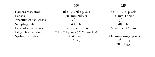
Parameters for the PIV and LIF measurements.
 $\eta$
and
 $\eta _B$
denote the Kolmogorov and Batchelor length scales, respectively. These scales are estimated at the centreline for all the streamwise locations measured in the present study.

A 540 nm short-pass optical filter was placed in front of the PIV camera (Phantom VEO340L), allowing the Mie scattering light to pass and rejecting the fluorescent light. For the LIF camera (Phantom V711), a 540 nm long-pass optical filter was used to capture only the fluorescent light. The two cameras were arranged along the same side of the laser sheet and a semi-transparent-semi-reflective mirror was used to split the light into two parts (figure 1
a). Calibration was performed using the same calibration target (LaVision) for both the PIV and LIF measurements. In figure 1(b,c), we show the image of the fluorescence field and the image of seeding particles. The field of view (FOV) of the LIF camera is 66 mm
 $\times$
105 mm in the streamwise and radial directions respectively, and is centred around the jet axis. The PIV only measures the upper half of the jet thanks to the fact that the jet is axisymmetric, the FOV of the PIV camera is 38 mm
 $\times$
61 mm, and its size and position relative to the FOV of the LIF is shown by a rectangle in figure 1(c). The two cameras and the laser were synchronised such that the velocity and scalar fields could be simultaneously measured. The specific parameters of PIV and LIF are listed in table 1. The velocity and scalar concentration fields were recorded at a sampling rate of 400 Hz, with a time interval of 2.5 ms between adjacent velocity/scalar concentration fields, which is smaller than the Kolmogorov time scale in all our measurements, indicating that our PIV/LIF measurement is time-resolved. Both cameras are operated in double-frame mode and we used the first frame of the LIF image to calculate the scalar concentration. Each PIV/LIF measurement comprised 3000 image pairs, resulting in 3000 time-resolved instantaneous velocity and concentration fields. Six independent measurements were performed under the same experimental condition, yielding a total of 18 000 velocity and concentration fields, which are sufficient for the subsequent analysis. The acquired tracer particle image pairs were processed by a recursive iterative interrogation scheme (LaVision, DaVis 8.4.0). The initial correlations were performed with a
 $48 \times 48$
pixel interrogation window, followed by a
 $24 \times 24$
pixel window, and with a 75
 $\%$
overlap in each interrogation step. The instantaneous velocity map contains
 $ 264 \times 423$
(
 $ x{-}r$
) vectors, with a vector spacing of 0.143 mm. The spurious velocity vectors was less than 1
 $\%$
, which was detected by a
 $5 \times 5$
median test and then replaced by linear interpolation around neighbour vectors. The accuracy of the particle displacement was estimated to be around 0.1 pixel.
To relate the light intensity with the actual concentration of the scalar, a pixel-by-pixel calibration was performed. First, the background intensity
 $\overline {I_{ {bg}}}(x,r)$
was obtained by averaging 1000 snapshots taken when no dye is added to the tank, where the bar denotes the time average. Then, the tank was filled with a well-mixed and known concentration (smaller than 80 ppb) rhodamine 6G solution. We captured 1000 snapshots to calculate the average intensity of the fluorescence,
 $ \overline {I_{ {cal}}}(x,r)$
. This process was repeated six times using six different concentrations of rhodamine 6G solutions. The background subtracted average light intensity
 $\overline {I_{ {cal}}}(x,r) - \overline {I_{ {bg}}}(x,r)$
should depend linearly on the scalar concentration. Finally, the instantaneous scalar concentration
 $ \phi _{R}(x,r)$
(the subscript
 $_{R}$
denotes rhodamine 6G) can be obtained using the following relation:
 \begin{equation} \frac {\phi _{R}(x,r)}{\phi _{R, {cal}}(x,r)} = \frac {\overline {I_{ {samp}}}(x,r) - \overline {I_{ {bg}}}(x,r)}{\overline {I_{ {cal}}}(x,r) - \overline {I_{ {bg}}}(x,r)}. \end{equation}
For accurate scalar concentration measurement, the laser intensity was kept the same during calibration and experiments.
Several factors, including light attenuation, secondary fluorescence effects and luminous efficiency, can affect the accuracy of the LIF (Baj et al. Reference Baj, Bruce and Buxton2016). However, in our experiment, we employed fluorescent dye at extremely low concentrations (linear region) and the above-mentioned effects are negligible (Parker et al. Reference Parker, Burridge, Partridge and Linden2020). Nevertheless, noise introduced by issues like laser intensity variation during the measurement can affect the final concentration field. To mitigate this noise, we applied a
 $3\times 3$
pixel median filter to smooth the measured concentration field. The scalar concentration has a single-pixel resolution (around
 $0.6{-}1.4\eta$
), and the spatial resolution of the velocity measurement is around
 $3{-}7 \eta$
. In the above,
 $\eta$
is estimated at the jet centreline for all the streamwise locations we measured in this study. The spatial resolution of our LIF measurement is sufficient to resolve the TNTI (Westerweel et al. Reference Westerweel, Fukushima, Pedersen and Hunt2009; Mistry et al. Reference Mistry, Philip, Dawson and Marusic2016; Kohan & Gaskin Reference Kohan and Gaskin2020).
(a) Instantaneous concentration field, normalised by the averaged centreline scalar concentration
 $\overline {\phi _{R,c}}$
and shown in logarithmic scale, in the pure water jet at
 $Re=7075$
. (b) Velocity field is superimposed on the concentration field and the arrow length represents the magnitude of velocity. (c,d) and (e,f) Same as panels (a) and (b) but for
 $Wi = 36.7$
and 85.6, respectively.

Figure 2 shows typical examples of the instantaneous scalar concentration and velocity vector fields measured in the far field (
 $45\lt x/D\lt 67$
) of a pure water jet and two polymer-laden jets. The scalar concentration field provides a clear visualisation of the vortices generated by the flow. It is evident that turbulent mixing is significantly suppressed with polymer additives, resulting in more unmixed low-concentration and high-concentration fluid clumps concentrated near the centreline in the polymer-laden jet. Compared with the pure water case, high-concentration passive scalar can even be observed near the turbulent/non-turbulent boundary in the polymer-laden jet. It is also observed that the scalar field and vortices are elongated along the streamwise direction (Guimarães et al. Reference Guimarães, Pimentel, Pinho and da Silva2020; Peng et al. Reference Peng, Zhang and Xi2023). The velocity field appears smoother with polymer additives, in line with previous observation that polymers suppress small-scale fluctuations (Zhang & Xi Reference Zhang and Xi2022).
To reveal the effects of polymers on the multi-scale nature of turbulence, we also measured the turbulent kinetic energy spectra. The resolution of the PIV camera (Phantom, VEO340L) was deliberately reduced to
 $144\times 800$
pixels, thereby enabling a much higher sample rate of
 $2000$
Hz, approximately
 $10$
times faster than the smallest time scale at
 $x/D=56$
. The captured image pairs were processed using the same method outlined before, yielding a thin slab of velocity field in the radial direction. Each measurement, lasting
 $80$
seconds, was repeated
 $7$
times. For each measurement, a time series was constructed from the measured velocity field at a fixed location and a direct Fourier transformation was subsequently applied. As we have seven segments of velocity measurements, the final velocity power spectrum is obtained by averaging the seven power spectra from those seven velocity segments. The high-frequency noise plateau of the power spectra from the PIV measurement was corrected using the method proposed by Oxlade et al. (Reference Oxlade, Valente, Ganapathisubramani and Morrison2012).
2.3. Experimental parameters
In our previous study (Peng et al. Reference Peng, Zhang and Xi2023), we used full-field PIV measurements to clearly demonstrate that polymer-laden jet evolves from the entrainment reduction regime near the jet exit to the entrainment enhancement regime further downstream, compared with the pure water case. We also found that the properties of the polymer-laden jet has very strong dependence on the Weissenberg number
 $Wi$
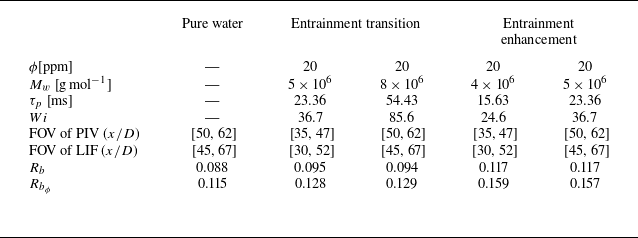
(Peng et al. Reference Peng, Zhang and Xi2023). Therefore, in this study, we performed four sets of PIV and LIF measurements with different
 $Wi$
and downstream locations, but at a fixed Reynolds number
 $Re = 7075$
and concentration
 $\phi =20$
ppm (parts per million by weight) (see table 2). The
 $Wi$
was varied by using different molecular weights
 $M_w$
of PEO, and these ranged from
 $24.6$
to
 $85.6$
. For the polymer solutions used here, the viscosity is practically the same as that of the solvent and the shear thinning effect is negligible (see Appendix A).
PIV and LIF measurement details.
 $\phi$
,
 $ M_{w}$
,
 $\tau _p$
and
 $Wi$
denote the polymer concentration, molecular weight of the PEO, relaxation time of the PEO and Weissenberg number, respectively. The positions for the PIV and LIF measurements are also specified. Here
 $R_{b}$
and
 $R_{b_{\phi }}$
are the spreading rates of the velocity and scalar fields, respectively.

The instantaneous velocity
 $U_i(x, r)$
(
 $ i = x, r$
) can be decomposed into time-averaged
 $\overline {U_i}(x, r)$
and fluctuation
 $u_i(x, r)$
components, i.e.
 $U_x(x, r) = \overline {U_x}(x, r) + u_x(x, r)$
. Similarly, the scalar concentration
 $\phi _{R}$
is decomposed into the time-averaged part
 $\overline {\phi _{R}}$
and the fluctuating part
 $\phi _{R}^{\prime }$
. The effects of polymer additives at different
 $Wi$
on the mean and fluctuation velocity and scalar fields are discussed in Appendix B. The spreading rate is the slope of the jet half-width. It is necessary to mention that the
 $Wi=24.6$
case at
 $x/D=[35,47]$
and the
 $Wi=36.7$
case at
 $x/D=[50,62]$
are in the entrainment enhancement regime, where the spreading rate is approximately
 $33\,\%$
larger than that of the pure water case; while the
 $Wi=36.7$
case at
 $x/D=[35,47]$
and the
 $Wi=85.6$
case at
 $x/D=[50,62]$
are in a transition regime, where the spreading rate is slightly larger than that of the pure water case; see table 2. The entrainment reduction regime is not investigated here since the measured TNTI through LIF measurement is discontinuous in the central plane due to the out-of-plane motion of the jet most of the time. This regime has been investigated in great detail by direct numerical simulation (DNS) by Abreu et al. (Reference Abreu, Pinho and da Silva2022).
The average kinetic energy dissipation rate
 $\varepsilon _{d}$
is calculated from the velocity gradient tensor under the axisymmetric hypothesis (Xu & Chen Reference Xu and Chen2013), which is expressed as
 \begin{equation} \varepsilon _{d, {axi}} = \nu \overline {8g_{rr}^2 -g_{xx}^2 + 2g_{xr}^2 + 2g_{rx}^2}, \end{equation}
where
 $\boldsymbol {g}_{ij}$
is the velocity gradient tensor. Due to the filtering effect of PIV algorithm, the measured
 $\varepsilon _{d}$
would be smaller than the ‘true’ dissipation rate (Lavoie et al. Reference Lavoie, Avallone, De Gregorio, Romano and Antonia2007). Since the filtering effect produces systematic error in both the Newtonian and the polymer-laden cases, we do not need to consider the filtering effect in our comparative study of the Newtonian and the polymer-laden jets. In addition, the measured
 $\varepsilon _{d}$
is non-zero in the non-turbulent region due to the measurement noise. This noise is Gaussian in nature and can be subtracted from the measured
 $\varepsilon _{d}$
(Westerweel et al. Reference Westerweel, Fukushima, Pedersen and Hunt2009). The
 $\varepsilon _{d}$
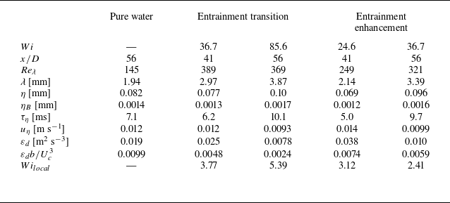
for all cases are listed in table 3.
Experimental parameters.
 $\phi$
,
 $ M_{w}$
,
 $\tau _p$
and
 $Wi$
denote the polymer concentration, molecular weight of the PEO, relaxation time of the PEO and Weissenberg number, respectively. The positions for the PIV and LIF measurements are also specified. Here
 $R_{b}$
and
 $R_{b_{\phi }}$
are the spreading rates of the velocity and scalar fields, respectively.

The basic flow parameters, including the Kolmogorov length scale
 $\eta = (\nu ^3/\varepsilon _{d})^{1/4}$
, Batchelor scale
 $\eta _B = \eta / \sqrt {Sc}$
, Kolmogorov time scale
 $\tau _\eta = (\nu /\varepsilon _{d})^{1/2}$
, Kolmogorov velocity scale
 $u_\eta = (\nu \varepsilon _{d})^{1/4}$
, Taylor micro length scale and Taylor-scale-based Reynolds number
 $Re_{\lambda } = u_{rms} \lambda / \nu$
, are listed in table 3, where
 $u_{rms}=\sqrt {(u_{x,rms}^2+2u_{r,rms}^2)/3}$
is the turbulent velocity fluctuation. Comparing the pure water case with the
 $Wi = 36.7$
and
 $ 85.6$
cases at
 $x/D=56$
(see table 3), it is clear that the kinetic energy dissipated by the fluid is suppressed, while the length scales (
 $\eta$
and
 $\lambda$
) and Reynolds number are larger. The above observations are consistent with the results reported in planar jet (Guimarães et al. Reference Guimarães, Pimentel, Pinho and da Silva2020) and isotropic turbulence (Rosti et al. Reference Rosti, Perlekar and Mitra2023).
2.4. Detection of the TNTI and determination of the entrainment velocity
The isosurface of passive scalar is extensively employed in detecting TNTI in Newtonian jets (Westerweel et al. Reference Westerweel, Fukushima, Pedersen and Hunt2009; Mistry et al. Reference Mistry, Philip, Dawson and Marusic2016; Kohan & Gaskin Reference Kohan and Gaskin2020). The same method is employed here. We first determine the concentration threshold to discriminate the turbulent/non-turbulent regions. The details can be found in Appendix C.1. In this study, the concentration threshold
 $\phi _R/\phi _{R,c}=0.18$
, where
 $\phi _{R,c}$
is the concentration at the centreline. Once the TNTI is determined, a local coordinate system along the TNTI can be established (see the inset of figure 3
a). Please note that
 $s_n \lt 0$
and
 $s_n \gt 0$
correspond to the non-turbulent and turbulent regions, respectively. Here,
 $\phi _R$
and out-of-plane vorticity
 $\omega$
can be further averaged condition on this local coordinate, which are denoted as
 $\langle \phi _R \rangle _{I}$
and
 $\langle \omega \rangle _{I}$
. Interestingly,
 $\langle \phi _{R}\rangle _{I}/\phi _{R, c}$
and
 $\left \langle \left | \omega \right |\right \rangle _I /(U_c/b)$
exhibit a sharp increase across the TNTI as shown in figure 3, demonstrating that the scalar can be used to detect the TNTI in the presence of polymers.
Conditionally averaged profiles of (a) scalar concentration,
 $\langle \phi _{R} \rangle _{I}/\phi _{R, c}$
, and (b) out-of-plane vorticity magnitude,
 $\langle | \omega |\rangle _I /(U_c/b)$
, along the local coordinate system, depicted as yellow arrows in the inset of panel (a). The rectangles, centred around
 $s_n=0$
, span a width of one Taylor length scale
 $\lambda$
.

The local entrainment velocity along the TNTI is measured by the interface tracking method proposed by Wolf et al. (Reference Wolf, Lüthi, Holzner, Krug, Kinzelbach and Tsinober2012). The displacement velocity of TNTI,
 $\boldsymbol {u_s}$
, has two contributions: the local fluid flow advection,
 $\boldsymbol {u_I}$
, and local entrainment across the TNTI,
 $v_n$
. Consequently,
 $v_{n} \boldsymbol {s_{n}} = \boldsymbol {u_{s}} - \boldsymbol {u_{I}}$
. The same method can be applied to a filtered scalar and velocity fields to calculate the local entrainment velocity at scale
 $\Delta$
. More details on the determination of
 $v_n$
can be found in Appendix C.2.
3. Turbulence characteristics in polymer-laden jet
Turbulent flow and entrainment process are multi-scale in nature. It is found that polymers redistribute energy among different scales (Valente et al. Reference Valente, da Silva and Pinho2014; Zhang et al. Reference Zhang, Bodenschatz, Xu and Xi2021). The degree of polymer extension and, in turn, its back-reaction on the flow depend on the local Weissenberg number (Guimarães et al. Reference Guimarães, Pimentel, Pinho and da Silva2020, Reference Guimarães, Pinho and da Silva2022). Figure 4(a) shows the radial profiles of
 $Wi_{local}=\tau _p/\tau _\eta$
at
 $x/D=56$
. Here,
 $Wi_{local}$
gradually decays along the radial direction as can be expected. At a fixed
 $x$
, the interface is not immobile but fluctuates in the radial direction, so it will probe a different region of the flow. Thus, it is more instructive to calculate
 $Wi_{local}$
conditioned on the local coordinate system along the TNTI,
 $ \langle Wi_{local} \rangle _{I}$
, and this is shown in figure 4(b). The
 $ \langle Wi_{local} \rangle _{I}$
is nearly
 $0$
in the non-turbulent region (
 $s_n\lt 0$
), experiences a sharp increase within the interface and then mildly increases in the turbulent region (
 $s_n\gt 0$
). The
 $ \langle Wi_{local} \rangle _{I}$
for the
 $Wi=36.7$
and
 $85.6$
cases is larger than
 $1$
within the interface and in the turbulent region, where the local flow would be modified by polymers.
(a) Radial profiles of the local Weissenberg number,
 $Wi_{local}$
, as a function of
 $r/b$
at streamwise position
 $x/D=56$
. (b) Conditionally averaged local Weissenberg number on the TNTI,
 $ \langle Wi_{local} \rangle _{I}$
, as a function of the distance
 $s_n$
from the TNTI. The vertical bar in panel (b) has a width of
 $\lambda$
.

We compare the power spectra of turbulent velocity for pure water and polymer-laden jets at the same downstream location, as depicted in figure 5. At the centreline of a pure water jet, an inertial range with
 $-5/3$
scaling in the range of
 $10\lt f\lt 10^2$
Hz is observed (figure 5
a). In the dissipation range (
 $f\gt 10^2$
Hz), there is a rapid decay in energy content. With the addition of polymers, the
 $E(f)$
of
 $Wi=36.7$
pivots at a frequency
 $f_p\approx 35$
Hz. Above this frequency, the energy content of the small-scales (high frequency) motion is suppressed; while below
 $f_p$
, the energy content is augmented. The enhancement of large scales (low frequency) and suppression of small-scales motion aligns with previous findings in Rayleigh–Taylor turbulence (Boffetta et al. Reference Boffetta, Mazzino and Musacchio2011).
Power spectra of turbulent velocity at (a)
 $(x/D,r/b)=(56,0)$
, (b)
 $(x/D,r/b)=(56,0.5)$
and (c)
 $(x/D,r/b)=(56,1)$
for the pure water and
 $Wi=36.7$
cases.
 $-5/3$
denotes the inertial range scaling in Newtonian turbulence.
 $-2.38$
and
 $-3$
are scaling exponents reported in inertio-elastic turbulence.

In figure 5(a), we also show two reference slopes frequently reported in the literature:
 $-2.38$
and
 $-3$
. Zhang et al. (Reference Zhang, Bodenschatz, Xu and Xi2021) reported an exponent of
 $-2.38$
in von Kármán flow, which was later confirmed in numerical simulation (Rosti et al. Reference Rosti, Perlekar and Mitra2023). In viscoelastic Taylor–Couette flow, Moazzen et al. (Reference Moazzen, Lacassagne, Thomy and Bahrani2023) reported a decay exponent of
 $-2.3$
extracted from the spatiotemporal maps obtained by flow visualisation; Boulafentis et al. (Reference Boulafentis, Lacassagne, Cagney and Balabani2024) found that the scaling exponent is close to
 $-2.5$
. Valente et al. (Reference Valente, da Silva and Pinho2016) investigated a wide range of
 $Wi$
and found that the exponent first decreases from
 $-5/3$
to
 $-3$
and then increases back to
 $-5/3$
as
 $Wi$
grows. Other studies also pointed towards an exponent of
 $-3$
(Vonlanthen & Monkewitz Reference Vonlanthen and Monkewitz2013; Yamani et al. Reference Yamani, Keshavarz, Raj, Zaki, McKinley and Bischofberger2021; Guimarães et al. Reference Guimarães, Pinho and da Silva2022; Soligo & Rosti Reference Soligo and Rosti2023). It seems that the scaling exponent depends on
 $Re$
and
 $Wi$
, and even the flow investigated. Due to the relatively low
 $Re$
here, the scaling range spans less than one frequency decade, it is hard to determine the scaling exponent. However, faster decay of the spectra in the inertial range is consistently observed, implying that the nonlinear energy transfer of the fluid is depressed.
Moving from
 $r/b=0$
to
 $r/b=0.5$
(figure 5
b), a similar effect on small scales is observed. The energy content of large scales only slightly increases, not as dramatically as that at
 $r/b=0$
. Further away from the centreline (
 $r/b=1$
, figure 5
c), the velocity becomes more intermittent due to the presence of non-turbulent regions, as will be discussed in figure 7. A slight deviation from the
 $-5/3$
scaling in the Newtonian case is observed in figure 5(c), which may result from the small
 $Re_\lambda$
in this radial position. It can be concluded that while the dissipative scale motions are consistently depressed in the radial direction, the effect of polymers on the inertial and energy-containing ranges of the kinetic energy spectrum strongly depend on the local Weissenberg number
 $Wi_{local}$
. At the energy containing range of the spectrum, the turbulent energy is increased by the polymers.
4. Local entrainment along the turbulent/non-turbulent interface
As reported in our previous study (Peng et al. Reference Peng, Zhang and Xi2023), the polymer additives suppress entrainment in the near field of the jet. The entrainment reduction phenomenon was thoroughly investigated by Abreu et al. (Reference Abreu, Pinho and da Silva2022) and attributed to a smoother TNTI in the viscoelastic case. However, in the far field of a viscoelastic jet, the entrainment rate significantly increases. This section delves into the underlying mechanism in the entrainment transition and enhancement regimes.
4.1. Engulfment flux
Engulfment is the process that the non-turbulent ambient fluid is transported into the turbulent core region by the large-scale inviscid motion (Roshko Reference Roshko1976; Westerweel et al. Reference Westerweel, Fukushima, Pedersen and Hunt2009; Jahanbakhshi & Madnia Reference Jahanbakhshi and Madnia2016; Long et al. Reference Long, Wang and Pan2022). Figure 6 shows the binarised images of instantaneous scalar concentration snapshots at the threshold of
 $\phi _{R}/\phi _{R, c} = 0.18$
. The red lines depict the TNTI on both sides of the jet. The white clumps within the interfaces are unmixed fluids that are drawn from the non-turbulent region by the engulfment process and are named as bubbles (Westerweel et al. Reference Westerweel, Fukushima, Pedersen and Hunt2009; Long et al. Reference Long, Wang and Pan2022; Xu et al. Reference Xu, Long and Wang2023). As
 $Wi$
increases, more bubbles are engulfed into the turbulent region and the TNTI exhibits significant fluctuation in the radial direction.
TNTI at multi-scales. The binarised images of the filtered scalar field, with filter sizes of (a,c,e)
 $\Delta /\eta \approx$
3 and (b,d,f)
 $\Delta /\eta \approx$
80, correspond to the cases of (a,b) pure water, (c,d)
 $Wi=36.7$
and (e,f)
 $Wi=85.6$
. The red lines represent the TNTI and the black lines are the interface envelope. The interface envelope is shifted by 0.3 mm in the radial direction to distinguish it from the TNTI. The dotted lines are the jet centreline.

P.d.f.s of the radial position
 $r_{I}$
(normalised by the half-width
 $b$
) of the TNTI with different filter size: (a)
 $\Delta /\eta \approx$
3 and (b)
 $\Delta /\eta \approx$
80. The solid lines represent Gaussian distribution.

The radial position of TNTI relative to the centreline is defined as
 $r_I$
, as shown in figure 6(a). Figure 7 shows the probability density functions (p.d.f.s) of
 $r_I$
at
 $x/D=56$
, but with two filter sizes
 $\Delta /\eta \approx 3$
and 80. In our measurement, we will get two interfaces as depicted in figure 6: a top and bottom one with respect to the jet centreline. The p.d.f.s shown in figure 7 use
 $r_I$
of the top interface, and a similar result will be obtained when using the bottom one since the jet is axisymmetric. The p.d.f. of
 $r_{I}$
for the pure water jet approximately follows a Gaussian distribution as observed by Kohan & Gaskin (Reference Kohan and Gaskin2020), Westerweel et al. (Reference Westerweel, Fukushima, Pedersen and Hunt2009) and Mistry et al. (2019). In addition, the p.d.f. is negatively skewed, which is associated with the engulfment process (Long et al. Reference Long, Wang and Pan2022). Figure 7(a) also shows that the p.d.f. of
 $r_{I}$
is still approximately Gaussian in a polymer-laden jet, with the maximum probability happening at the same radial position as the Newtonian case when
 $r_I$
is normalised by the jet half-width
 $b$
. Please note that the p.d.f.s of
 $r_I$
at different
 $x$
collapse onto a master curve when
 $r_I$
is normalised by
 $b$
in the Newtonian case (Mistry et al. Reference Mistry, Philip, Dawson and Marusic2016). For the polymer-laden jet, the p.d.f. of
 $r_I$
is wider on the both sides of the tail, signalling stronger large-scale fluctuation of TNTI in the polymer-laden jet. There are even some events with
 $r_I\lt 0$
at high
 $Wi$
in figure 7, meaning that both interfaces are located on the same side relative to the jet centreline, i.e.
 $r_I\lt 0$
for both interfaces. This phenomenon, however, is rarely observed in a Newtonian jet. At a larger filter size (figure 7
b), observations similar to those in figure 7(a) are noted. The above result indicates that large scale motions play an important role on increasing the motion of TNTI.
The centroid and area
 $S$
of the bubbles within TNTI can be readily estimated from figure 6(a,c,e), with
 $\sqrt {S}$
being taken as the characteristic size of the bubble. The p.d.f.s of bubble centroid radial position
 $r_{bub}$
and bubble size
 $\sqrt {S}$
are shown in figure 8. As
 $Wi$
increases, more bubbles appear near the jet centreline, corroborating the direct observations in figure 6(a,c,e). In the Newtonian case, bubbles are predominantly near the TNTI, with rare occurrences of bubbles at the centre (Xu et al. Reference Xu, Long and Wang2023). However, in the
 $Wi=85.6$
case, we can frequently observe bubbles in the centre. This phenomenon can be attributed to two processes. On one hand, polymers enhance the large scale motion, which results in higher radial position fluctuation of TNTI as shown in figure 7. When the TNTI is close to the centreline, the ambient non-turbulent fluid is more likely to be engulfed into the centre. On the other hand, polymers suppress the small scales, which reduces small-scale mixing. In that way, a bubble can persist for a longer time and be advected to the centre before being digested by the turbulent motion in the core region. Similarly, in figure 9, we also present the p.d.f.s of scalar concentration
 $\phi _{R}/\phi _{R, c}$
sampled on the turbulent core region. The probabilities of both low and high concentrations increase with
 $Wi$
, as indicated by the larger standard deviation (std) of
 $\phi _{R}/\phi _{R, c}$
. The coexistence of low and high scalar concentrations within the turbulent core region suggests that the small-scale mixing is hindered by polymers, aligning with the measured power spectra of turbulent velocity. It should be noted that scalars with
 $\phi _{R}/\phi _{R, c}\lt 0.18$
are located inside the bubbles. The larger probability of
 $\phi _{R}/\phi _{R, c}\lt 0.18$
also signifies more bubbles in the turbulent core region. The p.d.f.s of the bubble size are depicted in figure 8(b), where the p.d.f.s nearly overlap. The bubble size follows a power-law distribution with an exponent of
 $-3$
, a scaling close to that reported in the distribution of the size of the irrotational fluid region within the turbulent core (da Silva et al. Reference da Silva, Taveira and Borrell2014b
).
(a) P.d.f.s of the radial position of the bubble centroid. (b) P.d.f.s of the bubble size within the turbulent region.

P.d.f.s of the scalar concentration
 $\phi _{R}/\phi _{R, c}$
, sampled within the TNTI. The standard deviations of
 $\phi _{R}/\phi _{R, c}$
are also indicated in the legend. The vertical red line represents the scalar concentration threshold
 $\phi _{R}/\phi _{R, c}=0.18$
used in this study.

In the viscoelastic jet, more bubbles are engulfed into the turbulent region. One may wonder whether polymers have some effects on these bubbles or not. Figure 10 presents the mean streamwise velocity and out-of-plane vorticity within the bubbles, normalised by
 $U_c$
and
 $U_c/b$
, respectively, i.e.
 $ \overline {U_{x, bub}}/U_c$
and
 $\overline {\left | \omega \right |_{bub}}/(U_c/b)$
. For the mean streamwise velocity, we find that
 $ \overline {U_{x, bub}}/U_c$
exhibits a similar trend and magnitude with the mean streamwise velocity
 $ \overline {U_{x}}/U_c$
. However, the out-of-plane vorticity,
 $\overline {\left | \omega \right |_{bub}}/(U_c/b)$
, remains nearly constant within error bars in the radial direction. These observations suggest that while bubbles have gained momentum from the background turbulence, they have not mixed with the surrounding fluid to acquire more vorticity, indicating that engulfment is an inviscid process. Polymers augment the large-scale inviscid motion of turbulence, resulting in more bubbles being engulfed into the turbulent region. It is also interesting to note that
 $\overline {\left | \omega \right |_{bub}}/(U_c/b)$
in the viscoelastic case seems to be suppressed compared with the Newtonian case, though there are large error bars of the data. This behaviour indicates that when bubbles get across the TNTI, they acquire less vorticity in the presence of polymer, which may be related to the depression of vorticity production or diffusion by polymers (Cai et al. Reference Cai, Li and Zhang2010; Guimarães et al. Reference Guimarães, Pinho and da Silva2022).
Radial profiles of (a) the normalised streamwise velocity
 $ \overline {U_{x, bub}}/U_c$
and (
 $ b$
) the normalised out-of-plane vorticity
 $\overline {| \omega |_{bub}}/(U_c/b)$
in the bubbles. For comparison, the mean streamwise velocity
 $ \overline {U{x}}/U_c$
and out-of-plane vorticity
 $\overline {| \omega |}/(U_c/b)$
from the pure water case are also depicted, represented by red squares. The error bars in panel (a,b) denote one standard deviation. The large error bars of
 $\overline {| \omega |_{bub}}/(U_c/b)$
near
 $r/b\approx 0$
and
 $r/b\approx 3$
result from the limited data at these radial positions.

The observed phenomena suggest that polymer additives enhance the engulfment process due to the augmented large-scale inviscid motion. It is essential to determine the fraction of the total entrainment flux contributed by the engulfment flux. Westerweel et al. (Reference Westerweel, Fukushima, Pedersen and Hunt2009) proposed that all unmixed low-concentration fluids within the TNTI envelope, formed by the junction of the outermost part of TNTI (refer to the black lines in figure 6
a,c,e), result from engulfment. The total mass flux, denoted as
 $ Q$
, is expressed as
 \begin{equation} Q = 2\pi \rho \int _{0}^{\infty }\overline {U_{x}(r)} r\ \mathrm {d}r=2\pi \rho U_cb^2\int _{0}^{\infty }\xi f(\xi ) \mathrm {d}\xi , \end{equation}
where
 $U_c$
is the mean streamwise velocity at the centreline,
 $\xi =r/b$
is the scaled radial position and
 $f(\xi )=\overline {U_x}(\xi )/U_c$
is the scaled mean streamwise velocity. The entrainment rate
 ${\textrm { d}Q}/{\textrm { d}x}$
is the slope of total mass flux, i.e.
 \begin{equation} \frac {\textrm { d}Q}{\textrm { d}x} = 2\pi \rho (U_cb)\frac {\textrm { d}b}{\textrm { d}x}\int _{0}^{\infty }\xi f(\xi ) \mathrm {d}\xi . \end{equation}
Here,
 $U_cb$
is constant along the streamwise direction since the momentum is conserved (Peng et al. Reference Peng, Zhang and Xi2023). Also,
 $f(\xi )$
is the same for both Newtonian and viscoelastic jets (see appendix B). Thus,
 ${\textrm { d}Q}/{\textrm { d}x}$
is proportional to
 ${\textrm { d}b}/{\textrm { d}x}$
. For the interior of the TNTI envelope, the enclosed jet mass flux
 $ Q_{ {jet}}$
is defined as
 \begin{equation} Q_{ {jet}} = 2\pi \rho \int _{0}^{\infty }\overline {U_{x}(r)}\mathrm {p}_{ {jet}}(r)r\ \mathrm {d}r, \end{equation}
where
 $ \mathrm {p}_{ {jet}}(r)$
represents the probability that the jet is within the TNTI envelope at the radial position
 $r$
. The contribution of engulfment can be estimated from the volume of the unmixed low-concentration fluids within the TNTI envelope. Consequently, the engulfment mass flux,
 $ Q_{ {engulf}}$
, can be estimated by the equation,
 \begin{equation} Q_{ {engulf}} = 2\pi \rho \int _{0}^{\infty }\overline {U_{x}(r)}\mathrm {p}_{ {engulf}}(r)r\ \mathrm {d}r, \end{equation}
where
 ${p}_{ {engulf}}(r)$
denotes the probability that the low scalar concentration fluid, with
 $ \phi _{R}/\phi _{R, c} \lt 0.18$
, is within the TNTI envelope at the radial position
 $r$
. The mass fluxes
 $Q$
,
 $ Q_{ {jet}}$
and
 $ Q_{ {engulf}}$
at specific
 $x/D$
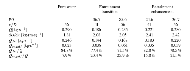
are tabulated in table 4. The results indicate that the contribution of engulfment in pure water jet,
 $ Q_{ {engulf}}/Q$
, is 7.9
 $ \%$
, in good agreement with previous study (Westerweel et al. Reference Westerweel, Fukushima, Pedersen and Hunt2009). This suggests that engulfment is not the primary mechanism in the entrainment process of a Newtonian jet, a conclusion also reported in studies on a synthetic jet and boundary layer (Long et al. Reference Long, Wang and Pan2022; Xu et al. Reference Xu, Long and Wang2023), where the entrainment flux due to engulfment does not exceed
 $10\,\%$
.
Mass flux in the pure water and polymer-laden jets. Here
 $Q$
,
 $ Q_{ {jet}}$
and
 $ Q_{ {engulf}}$
denote the total mass flux, mass flux within the TNTI envelope and engulfment mass flux, respectively.

In the viscoelastic case, the contribution of engulfment to entrainment,
 $ Q_{ {engulf}}/Q$
, increases with
 $Wi$
. The maximum contribution is approximately
 $25.9\,\%$
in the
 $Wi=85.6$
case. Despite the significant enhancement of the contribution due to engulfment compared with the Newtonian case, we conclude that engulfment is still not the primary mechanism in the entrainment of a polymer-laden jet over the parameter range investigated here. In the entrainment enhancement regime, the engulfment process is significantly increased, suggesting the importance of the engulfment process in enhancing the entrainment. It would be interesting to further increase
 $Wi$
to examine the role of engulfment in the entrainment of a polymer-laden jet. However, it should be noted that in experiments, polymer chains may degrade due to strong shear at higher
 $Wi$
values.
Considering the
 $Wi=36.7$
case in the entrainment transition regime (
 $x/D=41$
) and entrainment enhancement regime (
 $x/D=56$
), although
 $Q$
,
 $Q_{ { jet}}$
and
 $Q_{{engulf}}$
all increase in the streamwise direction, the jet and engulfment contribution to the total flux remain relatively constant in the streamwise direction (refer to the third and sixth rows of table 4). This suggests that the engulfment process does not play a role in governing the change from the entrainment transition regime to the entrainment enhancement regime. It should be emphasised here that we use ‘entrainment enhancement regime’ to represent that in that regime, the entrainment rate is enhanced, not the entrainment itself (total mass flux). Actually, in the entrainment enhancement regime, the entrainment or the total mass flux
 $Q$
is reduced compared with that in the Newtonian jet (compare the fifth row with the second row of table 4). This is due to the fact that the entrainment is significantly reduced in the near field, which results in smaller
 $Q$
. Further downstream,
 $Q$
in the viscoelastic jet exceeds that in the Newtonian jet as shown in our previous study (Peng et al. Reference Peng, Zhang and Xi2023).
4.2. Entrainment flux along the turbulent/non-turbulent interface
In § 4.1, we analyse the impact of polymer additives on the engulfment process, where the ambient quiescent fluid parcels are engulfed into the turbulent core region by the large-scale inviscous eddies. However, recent studies showed that the entrainment is a multi-scale process along the TNTI (Meneveau & Sreenivasan Reference Meneveau and Sreenivasan1990; Mistry et al. Reference Mistry, Philip, Dawson and Marusic2016), with the entrainment rate depending on the surface area
 $S$
and entrainment velocity
 $V_n$
. At the smallest length scale (of order of
 $\eta$
),
 $V_n$
is small but is balanced by a large
 $S$
since the surface is convoluted. While at large scales,
 $V_n$
is large but is balanced by a small
 $S$
since the surface is smooth. Hence, the entrainment rate,
 $S(\Delta )V_n(\Delta )$
, estimated at different scale
 $\Delta$
is scale-invariant. In the inertial range of scales, the TNTI is multi-fractal, i.e.
 $S(\Delta )\sim \Delta ^{-D_3}$
with the scaling exponent
 $2.3\lt D_3\lt 2.4$
(Mistry et al. Reference Mistry, Philip, Dawson and Marusic2016). Accordingly,
 $V_n(\Delta )\sim \Delta ^{D_3}$
in the inertial range. In this section, we will delve into the effects of polymers on the those two contributing factors:
 $S(\Delta )$
and
 $V_n(\Delta )$
.
In our experiment, two-dimensional velocity and scalar concentration fields are available, from which TNTI length
 $L_{TNTI}$
and local entrainment velocity
 $v_n$
projected on the
 $x{-}r$
plane can be estimated. Given the axisymmetric nature of the jet, the mean entrainment velocity is given by
 \begin{equation} V_{n} = \overline {\left [\frac {\int _{0}^{L_{TNTI}} (-v_{n}) r_{I} \mathrm {d}s}{\int _{0}^{L_{TNTI}} r_{I} \mathrm {d}s}\right ]}, \end{equation}
which is integrated on the local coordinate along the TNTI. From the two-dimensional measurement,
 $L_{TNTI}(\Delta )\sim \Delta ^{2-D_3}$
and
 $V_n(\Delta )\sim \Delta ^{D_3-2}$
in the Newtonian case.
In figure 11(a,b), we show
 $L_{TNTI}$
and
 $V_n$
of the pure water case. For the pure water case,
 $L_{TNTI}$
scales with the filter size
 $\Delta$
in the log-log plot between
 $\lambda$
and
 $b$
(we take
 $b$
as the integral length scale), i.e.
 $L_{TNTI}\sim \Delta ^{2-D_3}$
with
 $D_3\approx 2.31$
. Here,
 $V_n$
increases with
 $\Delta$
and follows a power-law scaling in the inertial range with an exponent
 $D_3-2\approx 0.31$
. Those two scalings,
 $L_{TNTI}\sim \Delta ^{-0.31}$
and
 $V_n\sim \Delta ^{0.31}$
, together make the entrainment rate,
 $L_{TNTI}(\Delta )V_n(\Delta )$
, independent of scales, which was corroborated in experiment by Mistry et al. (Reference Mistry, Philip, Dawson and Marusic2016). We also note that the scaling range of
 $V_n$
is shorter than that of
 $L_{TNTI}$
, probably due to the small Reynolds number (
 $Re_\lambda =106$
at
 $x/D=56$
) in our study.
(a,c) TNTI length,
 $L_{TNTI}$
(normalised by
 $ L_x$
), and (b,d) mean entrainment velocity,
 $V_n$
(normalised by the mean centreline axial velocity
 $U_c$
), as a function of the filter size
 $\Delta$
.
 $L_x = 12 D$
represents the length of the measurement region along the flow direction. The two vertical bars represent the Taylor scale
 $\lambda$
(left) and the integral scale
 $b$
(right) within the measurement range. The black horizontal bar denotes the large scale entrainment coefficient of the pure water case in the self-similar regime. The green horizontal bar denotes the large scale entrainment coefficient of the polymer-laden case in the entrainment enhancement regime.

We start our analysis with the
 $Wi=36.7$
case in the entrainment transition regime at
 $x/D=[35,47]$
. The scaling exponent of
 $L_{TNTI}$
is altered by polymers, with a least-square fit yielding
 $2-D_3\approx -0.23$
. The corresponding
 $D_3\approx 2.23$
, indicating that the interface is smoother than that of the pure water case at small scales, in line with the numerical simulation (Abreu et al. Reference Abreu, Pinho and da Silva2022). The scaling exponent of
 $V_n$
changes accordingly, i.e.
 $V_n\sim \Delta ^{0.23}$
, despite the short scaling range. The multi-scale nature of the entrainment velocity in the viscoelastic case has not been investigated in previous study. Previous studies showed that the small-scale end of the inertial range will be modified with the addition of polymers and a new scaling range will emerge between the inertial and dissipation ranges at high elasticity (Valente et al. Reference Valente, da Silva and Pinho2016; Zhang et al. Reference Zhang, Bodenschatz, Xu and Xi2021). In turbulent jet flow, the scaling of the power spectrum of fluctuating velocity is altered, as has already been observed in figure 5(a,b). The change in the energy content among different scales will then modulate the scaling of
 $L_{TNTI}$
and
 $V_n$
in the polymer-laden jet.
At the small-length scale (
 $\Delta \lt \lambda$
), the inertial force can be neglected and the viscous diffusion becomes dominated. Hence, the viscous nibbling is the dominating mechanism of entrainment at small scales. In the Newtonian jet, enstrophy production, viscous diffusion and viscous dissipation contribute to the nibbling process (Holzner & Lüthi Reference Holzner and Lüthi2011; Wolf et al. Reference Wolf, Lüthi, Holzner, Krug, Kinzelbach and Tsinober2012; Watanabe et al. Reference Watanabe, Sakai, Nagata, Ito and Hayase2014; Abreu et al. Reference Abreu, Pinho and da Silva2022; Long et al. Reference Long, Wang and Pan2022). In viscoelastic fluid, Abreu et al. (Reference Abreu, Pinho and da Silva2022) reported that vorticity diffusion induced by polymer elastic stress also contributes to the nibbling velocity. With the addition of polymers, the small-scale fluctuation is suppressed (Valente et al. Reference Valente, da Silva and Pinho2016; Zhang et al. Reference Zhang, Bodenschatz, Xu and Xi2021; Zhang & Xi Reference Zhang and Xi2022) and the enstrophy production is also inhibited by polymers (Cai et al. Reference Cai, Li and Zhang2010; ur Rehman et al. Reference ur Rehman, Lee and Lee2022). We would then expect that the contributions from enstrophy production, viscous diffusion and viscous dissipation are depressed accordingly, as was observed by Abreu et al. (Reference Abreu, Pinho and da Silva2022). At the smallest scale we resolved here (
 $\Delta \approx$
 $3\eta$
), we find that
 $V_n$
, however, is larger than that of the pure water case, implying that polymer elastic stress contributes to increase the entrainment velocity, i.e. elastic stress plays an important role in the local entrainment at small scales in the polymer-laden jet, in line with previous simulation (Abreu et al. Reference Abreu, Pinho and da Silva2022).
For the
 $Wi=36.7$
case in the entrainment enhancement regime at
 $x/D=[50,62]$
, the scalings of
 $L_{TNTI}$
and
 $V_n$
are almost the same as those of the pure water case in figure 11(a,b). This observation seems contradictory with the enhanced
 $V_n$
and modified power spectrum in figure 5, all pointing to a different scaling of
 $L_{TNTI}$
and
 $V_n$
. However, two important features need to be noted: (i) the radial position of TNTI is larger than
 $b$
, i.e.
 $r_I\gt b$
, most of the time; (ii) the flow becomes weaker along the radial direction as shown in figure 4. The whole range of scales including the scaling exponent are altered by polymers near the centre (
 $0\leqslant r/b \leqslant 0.5$
), while polymers primarily affect the dissipative scales when
 $r/b\geqslant 1$
, and the scaling exponent remains nearly unaffected. The same scaling of
 $L_{TNTI}$
and
 $V_n$
for the
 $Wi=35.6$
case at
 $x/D=[50,62]$
can be understood from the fact that, in this downstream region and near the TNTI, polymers suppress the dissipative scale fluctuations but will not modify the scaling for scales between the dissipative and integral length scales.
Morton et al. (Reference Morton, Taylor and Turner1956) proposed that
 $V_{n}$
is proportional to
 $U_c$
, i.e.
 $V_n = \alpha U_c$
with
 $ \alpha$
being the entrainment coefficient, and the entrainment rate is
 $b(x)\alpha U_c(x)$
at the large scale. In our previous study, we have shown that
 $b(x)U_c(x)$
is constant in the streamwise direction and will not be changed by polymers (Peng et al. Reference Peng, Zhang and Xi2023). The entrainment rate thus merely depends on the
 $ \alpha$
. From figure 11(b), we find that
 $V_n$
increases with
 $\Delta$
and approaches a constant when
 $\Delta$
is close to
 $b$
. The plateau, marked with a horizontal bar, gives the entrainment coefficient
 $ \alpha$
. For the Newtonian case,
 $\alpha = 0.036 \pm 0.001$
(black horizontal bar), in agreement with the value reported by Mistry et al. (Reference Mistry, Philip, Dawson and Marusic2016). In the entrainment enhancement regime (
 $Wi=36.7$
case at
 $x/D=[50,62]$
),
 $\alpha = 0.050 \pm 0.001$
, which is increased by approximately
 $38\,\%$
compared with the Newtonian case. In the transition regime (
 $Wi=36.7$
case at
 $x/D=[35,47]$
),
 $V_{n}/U_c$
at small scale is comparable to that at
 $x/D=[50,62]$
. However, due to the different scaling of
 $V_{n}$
,
 $V_{n}$
at
 $x/D=[35,47]$
gradually departs from that at
 $x/D=[50,62]$
for
 $\lambda \lt \Delta$
 $\lt b$
. Additionally,
 $\alpha$
at
 $x/D=[35,47]$
is only slightly larger when compared with the Newtonian case.
Comparing
 $L_{TNTI}$
and
 $V_n$
in the entrainment transition and enhancement regimes at
 $Wi=36.7$
, we learn that polymers alter the scaling of
 $L_{TNTI}$
and
 $V_n$
in the entrainment transition regime, and the scaling remains the same in the entrainment enhancement regime. This may be related to a different degree of polymer elasticity. In the entrainment transition regime, the turbulence intensity is high enough to stretch polymers to a large degree, which in turn alter the scaling of
 $L_{TNTI}$
and
 $V_n$
(Xi et al. Reference Xi, Bodenschatz and Xu2013; Valente et al. Reference Valente, da Silva and Pinho2014; Zhang et al. Reference Zhang, Bodenschatz, Xu and Xi2021). In the entrainment enhancement regime, turbulence decays so that the polymers are stretched to a less degree, then the back reaction is not strong enough to alter the scaling of
 $L_{TNTI}$
and
 $V_n$
in the inertial range. Guimarães et al. (Reference Guimarães, Pinho and da Silva2024) recently showed the existence of different regimes of polymer conformation as the flow evolves downstream, e.g. the high-elasticity and low-elasticity regions. The entrainment transition and enhancement regimes thus may correspond to the high-elasticity and low-elasticity regions of polymer conformation reported in their study, respectively.
The
 $L_{TNTI}$
and
 $V_n$
from different Weissenberg number cases are shown in figure 11(c,d). We first compare
 $L_{TNTI}$
and
 $V_n$
from the
 $Wi=24.6$
case at
 $x/D=[35,47]$
and the
 $Wi=36.7$
case at
 $x/D=[50,62]$
, which are both in the entrainment enhancement regime. It is found that
 $L_{TNTI}$
and
 $V_n$
from those two cases overlap with each other. Our results show that not only the global statistics, such as the normalised mean velocity and velocity fluctuation profiles, but also the local properties, including the TNTI length and entrainment velocity, are independent of the Weissenberg number, further demonstrating the universal nature in the entrainment enhancement regime. We then compare
 $L_{TNTI}$
and
 $V_n$
from the
 $Wi=36.7$
and
 $Wi=85.6$
cases at the same downstream region (
 $x/D=[50,62]$
). At
 $x/D=56$
,
 $Wi_{local}$
in the
 $0\leqslant r/b \lt 2$
for the
 $Wi=85.6$
case is larger than
 $2.2$
, which is the
 $Wi_{local}$
at the centreline for the
 $Wi=36.7$
case (figure 4). Due to the larger
 $Wi_{local}$
, we observe that the scaling exponents of
 $L_{TNTI}$
and
 $V_n$
for the
 $Wi=85.6$
case are modified when compared with the
 $Wi=36.7$
case. The corresponding scaling exponent
 $D_3 \approx 2.27$
.
Entrainment velocity conditioned on the radial location of the TNTI
 $ - \langle v_n \rangle |_{r_{I}}P(r_I)$
at two filter sizes (a)
 $\Delta /\eta \approx$
3 and (b)
 $\Delta /\eta \approx$
80.

In the above, the enhanced
 $V_n$
at small scale is ascribed to the polymer elastic stress, as also reported in numerical simulation (Abreu et al. Reference Abreu, Pinho and da Silva2022). In a turbulent jet, the flow is inhomogeneous in the radial direction. Mistry et al. (Reference Mistry, Philip, Dawson and Marusic2016) studied the conditionally averaged value of
 $v_n$
on
 $r_I$
, denoted as
 $ - \langle v_n \rangle |_{r_{I}}$
. They found that the local entrainment is larger when TNTI is close to the centreline and
 $ - \langle v_n \rangle |_{r_{I}}$
monotonically decreases with
 $r_I$
. The local mean entrainment velocity at a specific
 $r_I$
also depends on the p.d.f. of
 $r_I$
(
 $P(r_I)$
), namely
 $ - \langle v_n \rangle |_{r_{I}} P(r_I)$
. Integrating
 $ - \langle v_n \rangle |_{r_{I}} P(r_I)$
in the radial direction yields the mean entrainment velocity. In figure 12, we compare
 $ - \langle v_n \rangle |_{r_{I}} P(r_I)$
between the pure water jet and the polymer-laden one. Here,
 $ - \langle v_n \rangle |_{r_{I}} P(r_I)$
for the polymer-laden jet is larger than that for the pure water one at the same
 $r_I$
, presumably due to the polymer elastic stress. There is also another contribution that needs to be stressed. We have observed that the tails of
 $P(r_I)$
becomes wider with the addition of polymers. The larger
 $ - \langle v_n \rangle |_{r_{I}}$
and higher probability of
 $P(r_I)$
near the centreline will also contribute to the enhanced entrainment velocity; see the
 $ - \langle v_n \rangle |_{r_{I}} P(r_I)$
curves within
 $0\lt r_I/b\lt 1$
in figure 12.
P.d.f.s of the local entrainment velocity
 $v_n$
at two filter sizes (a)
 $\Delta /\eta \approx$
3 and (b)
 $\Delta /\eta \approx$
60. The black curves represent Gaussian distribution.

Figure 13 depicts the p.d.f.s of the local entrainment velocity
 $v_{n}$
at both small (
 $\Delta /\eta \approx$
3) and large (
 $\Delta /\eta \approx$
60) scales. Please note that the mean entrainment velocity
 $V_n$
is of order of
 $u_\eta$
. The local
 $v_{n}$
acquire values an order of magnitude larger than
 $u_\eta$
, whose probability is much higher with respect to the Gaussian distribution (see the black lines in figure 13). The p.d.f.s are also negatively skewed, signifying the outward spreading tendency of the turbulent region (Holzner & Lüthi Reference Holzner and Lüthi2011; Wolf et al. Reference Wolf, Lüthi, Holzner, Krug, Kinzelbach and Tsinober2012; Krug et al. Reference Krug, Holzner, Lüthi, Wolf, Kinzelbach and Tsinober2015; Mistry et al. Reference Mistry, Philip, Dawson and Marusic2016; Long et al. Reference Long, Wang and Pan2022). In the polymer-laden jet, both tails of the p.d.f.s become wider, namely the local entrainment (
 $v_n\lt 0$
) and detrainment (
 $v_n\gt 0$
) velocity are both increased. Therefore, the behaviours of TNTI, including its radial position and velocity, are more intermittent in the viscoelastic jet as a result of the augmented large-scale motion.
5. Conclusions
We present an experimental study on the effects of polymer additive on the local entrainment process along the TNTI in the entrainment transition and enhancement regimes of a turbulent round water jet. We employ time-resolved simultaneous PIV and LIF to measure the velocity and scalar concentration fields. From the scalar concentration field, we detect the TNTI and engulfed ‘bubbles’. The entrainment velocity along the TNTI is determined using an interface-tracking method. By applying the spatial-filtering to the velocity and scalar concentration fields, we also analyse the geometrical feature of the TNTI and the entrainment velocity at multi-scales.
In polymer-laden water jets, polymers redistribute energy among different scales: reducing the energy content in dissipative scales and enhancing energy content in large scales. The latter induces more intermittent TNTI fluctuations in the radial direction and engulfs more bubbles into the turbulent region. Though the engulfment contribution to the total mass flux increases with
 $Wi$
, engulfment is still not the primary entrainment mechanism in polymer-laden water jets in the present parameter range. In addition, we also note that the engulfment contribution to the total mass flux remains nearly constant in the streamwise direction. Thus, engulfment is not related to the evolution from the entrainment transition regime to the entrainment enhancement regime.
The entrainment process is then investigated from the perspective of TNTI length and local entrainment velocity at multi-scales. The local entrainment velocity is increased in both regimes, which is caused by the contribution from the polymer elastic stress and more intermittent TNTI motion. The difference between the two regimes comes from the TNTI length. In the entrainment transition regime, polymers reduce the fractal dimension of TNTI and lead to a smaller interface length, consistent with previous studies (Guimarães et al. Reference Guimarães, Pimentel, Pinho and da Silva2020; Yamani et al. Reference Yamani, Keshavarz, Raj, Zaki, McKinley and Bischofberger2021; Guimarães et al. Reference Guimarães, Pinho and da Silva2025). In the entrainment enhancement regime, the fractal dimension of TNTI as well as the interface length are not altered by polymers. This difference may be traced to the degree of polymer elasticity, with high and low elasticity in the entrainment transition and enhancement regimes, respectively. Our results also show that, in the entrainment enhancement regime, the TNTI length and mean entrainment velocity, when properly normalised, are independent of the Weissenberg number, demonstrating the universal nature of polymer-laden jet in this regime. In addition, in the entrainment enhancement regime, the normalised velocity fluctuations and mean entrainment velocity of the viscoelastic jet are higher than that of the Newtonian jet.
Based on our experimental results and previous numerical simulations (Guimarães et al. Reference Guimarães, Pimentel, Pinho and da Silva2020, Reference Guimarães, Pinho and da Silva2022), the transition from the entrainment reduction regime to entrainment enhancement regime for large-
 $Wi$
jets can be understood as follows: (i) the initial depletion of small-scale motions caused by polymers and the subsequent attenuation of this effect in the very far field, where the local
 $Wi$
is small; (ii) the overall enhancement of large-scale engulfment at all regions (near field and far field) that is not attenuated in the very far field.
Acknowledgements
We are grateful to stimulating discussions with Prof. Jinjun Wang and acknowledge Prof. Chao Sun for the rheology measurement and Jia-Qi Ma for help in PIV and LIF measurements.
Funding
This work is financially supported by the National Natural Science Foundation of China (NSFC) through Grant Nos. 12388101, 12125204 and 12402298, and the 111 Project of China through Grant No. B17037.
Declaration of interests
The authors report no conflict of interest.
Appendix A. Viscosity of the polymer solution
The shear viscosity was measured by a Discovery HR1 rheometer (TA instruments) equipped with a cone-plate geometry. The cone is 40 mm in diameter and has an angle of
 $2^\circ$
, allowing for the shear rate in the range
 $6\lt \dot {\gamma }\lt 600$
s−1. The measured viscosity
 $\mu$
at 22
 $^{\circ }$
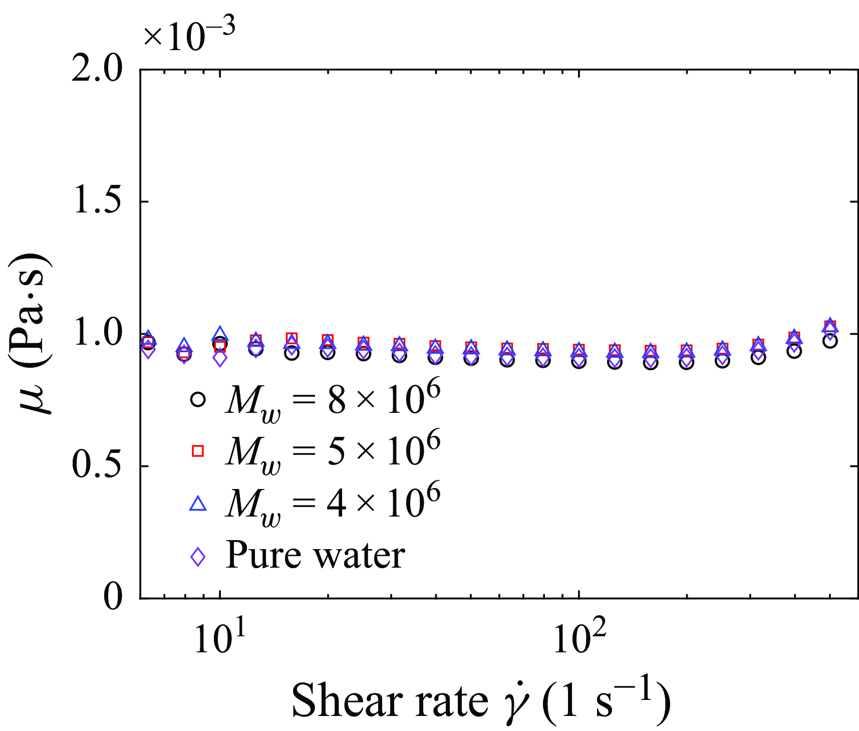
C is shown in figure 14. In our experiment, the polymer solutions are in the dilute regime and the viscosity change due to the addition of polymer additives can hardly be observed. Moreover, the viscosity remains nearly constant within the shear rate that can be realised in our rheometer. Therefore, the shear-thinning effect of polymer solutions is only marginal in our study (Deblais et al. Reference Deblais, Herrada, Eggers and Bonn2020).
Measured viscosity of pure water and polymer solutions (20 ppm) used in our experiment.

Appendix B. Velocity and scalar statistics
Figure 15(a) compares the streamwise evolution of the jet half-width
 $b$
obtained from local PIV measurements with the full-field velocity results reported by Peng et al. (Reference Peng, Zhang and Xi2023). Here,
 $b$
is defined as the radial distance at which the mean streamwise velocity decays to half of the local centreline value. The local PIV measured
 $b$
is consistent with the full-field results for both pure water and polymer solution jets. In the case of a pure water jet,
 $b$
scales linearly with the streamwise distance
 $x$
, exhibiting a spreading rate
 $R_{b}\approx$
0.088 (refer to Peng et al. (Reference Peng, Zhang and Xi2023) for more details). Following the approach of Guimarães et al. (Reference Guimarães, Pimentel, Pinho and da Silva2020), we applied a linear fit to
 $b$
in each local PIV measurement and
 $R_{b}$
for each position is listed in table 2. Among the four cases of polymer-laden jets measured in this study, two (
 $Wi = 24.6$
at
 $x/D = [35,47]$
and
 $Wi = 36.7$
at
 $x/D = [50,62]$
) exhibit a spreading rate of approximately 0.117 (33
 $ \%$
larger compared with the pure water jet), indicating that these polymer-laden jets have entered the entrainment enhancement regime. The other two polymer-laden jets (
 $Wi = 36.7$
at
 $x/D = [35,47]$
and
 $Wi = 85.6$
at
 $x/D = [50,62]$
) display a half-width spreading rate slightly larger than that of the pure water jet, suggesting that they are still in the transition range and have not yet entered the entrainment enhancement regime. For the
 $Wi=85.6$
case, the spreading rate is clearly reduced by the polymers in the near field at
 $20 \lt x/D \lt 35$
, in agreement with the DNS results of Guimarães et al. (Reference Guimarães, Pimentel, Pinho and da Silva2020) and the experiments of Yamani et al. (Reference Yamani, Keshavarz, Raj, Zaki, McKinley and Bischofberger2021).
(a) Variation of the jet half-width
 $b$
(normalised by the pipe diameter
 $D$
) along the flow direction for both the pure water and polymer-laden jets at different
 $Wi$
values. The hollow and solid symbols represent results from the full-field PIV of Peng et al. (Reference Peng, Zhang and Xi2023) and local PIV in this study, respectively. The solid and dashed lines are linear fits to
 $b$
in the self-similar region of the pure water jet and the polymer-laden jet at
 $Wi=24.6$
. Dashed lines with the same slope as that of the
 $Wi=24.6$
case are also shown for the
 $Wi=36.7$
and 85.6 cases. (b) Analogous to panel (a), but the half-width is defined using the scalar concentration.

Analogous to the half-width of the velocity field, we can define the half-width
 $b_{\phi _R}$
of the scalar concentration field, as depicted in figure 15(b). In the Newtonian case,
 $b_{\phi _R}$
increases linearly with
 $x/D$
, yielding a spreading rate of
 $R_{b_{\phi }} \approx 0.115$
, which is in line with the value reported by Mistry et al. (Reference Mistry, Philip, Dawson and Marusic2016). It is also observed that
 $R_{b_{\phi }}$
in the entrainment enhancement regime remains independent of
 $Wi$
, while the positions entering this regime shift to larger
 $x$
values as
 $Wi$
increases. In the entrainment enhancement regime (
 $Wi = 24.6$
at
 $x/D =$
[35, 47] and
 $Wi = 36.7$
at
 $x/D =$
[50, 62]),
 $R_{b_{\phi }} \approx 0.157$
, which is approximately
 $36\,\%$
larger than that of the pure water case. However, in cases that are still developing (
 $Wi = 36.7$
at
 $x/D =$
[35, 47] and
 $Wi = 85.6$
at
 $x/D =$
[50, 62]),
 $R_{b_{\phi }}$
values are slightly larger than that of the pure water jet.
Radial profiles of the normalised (a) mean axial velocity, (b) mean scalar concentration, (c) axial velocity fluctuation and (d) scalar concentration fluctuation.

Figure 16 presents the normalised mean and root-mean-square (r.m.s.) velocity and scalar profiles from the local PIV/LIF measurement. The velocity profiles, discussed in detail by Peng et al. (Reference Peng, Zhang and Xi2023), can be summarised as follows. First, the profiles
 $\overline {U_x}/U_c$
(figure 16
a) for pure water and polymer solutions at different downstream positions coincide with each other. Second, the profiles of the streamwise turbulent intensities
 $u_{x, rms}/U_c$
(figure 16
b) in the polymer-laden jets consistently exceed those in the pure water jet, evolving into a new self-similar state in the far field (as indicated by the black dashed line in figure 16
b). It is evident that the
 $u_{x, rms}/U_c$
profiles for the polymer-laden jets at
 $Wi = 24.6, x=40D$
and
 $Wi = 36.7, x=55D$
collapse together in the entrainment enhancement regime.
The mean scalar concentration profiles
 $\phi _{R}/\phi _{R,c}$
of both pure water and polymer-laden jets at various
 $x$
values exhibit a remarkable collapse when normalised by the local scalar half-width
 $b_{\phi _{R}}$
. These profiles can be approximately fitted by a Gaussian curve
 $\overline {\phi _R}/\phi _{R, c} =$
exp
 $(-0.69(r/b_{\phi _R})^2)$
, as indicated by the black line in figure 16(b). Figure 16(d) also presents the normalised r.m.s. scalar concentration profiles,
 $\phi ^{\prime }_{R, rms}/\phi _{R, c}$
, in the pure water and polymer-laden jets. Though
 $\phi _{R,rms}^{\prime } /\phi _{R,c}$
and
 $u_{x,rms}/U_c$
are both enhanced in the measurement position, the degree of enhancement differs. For the
 $Wi=85.6$
case,
 $\phi _{R,rms}^{\prime } /\phi _{R,c}$
shows the largest increase, while the increase in
 $u_{x,rms}/U_c$
is the smallest, indicating a qualitatively different effect of polymers on the velocity and scalar. The scalar field results are in agreement with the simulation results of passive scalar mixing reported by Guimarães et al. (Reference Guimarães, Pinho and da Silva2025), providing evidence for the employment of scalar to detect TNTI in viscoelastic jet flow.
Appendix C. Turbulent/non-turbulent interface
Various empirical methods have been proposed to detect the TNTI, including the isosurface of vorticity or velocity fluctuation (de Silva et al. Reference de Silva, Philip, Chauhan, Meneveau and Marusic2013; da Silva et al. Reference da Silva, Hunt, Eames and Westerweel2014a ; Watanabe et al. Reference Watanabe, Zhang and Nagata2018; Balamurugan et al. Reference Balamurugan, Rodda, Philip and Mandal2020). However, in PIV measurement near the TNTI, the particle displacement is small, resulting in large uncertainties in the measured velocity and vorticity. An alternative approach to detect TNTI is the isosurface of passive scalar, which has been extensively employed in experiments of Newtonian jet (Westerweel et al. Reference Westerweel, Fukushima, Pedersen and Hunt2009; Mistry et al. Reference Mistry, Philip, Dawson and Marusic2016; Kohan & Gaskin Reference Kohan and Gaskin2020). In Appendix B, we compare the statistics of velocity and scalar fields, showing that there are some similarities but also some differences between them. In this section, we will show that the passive scalar can still be used to detect TNTI, and introduce the method to measure the local entrainment velocity along the TNTI via time-resolved simultaneous velocity and scalar concentration fields.
C.1 Detection of the turbulent/non-turbulent interface
(a) Conditional averaged scalar concentration
 $ \widetilde \phi _{R}/\phi _{R, c}$
which is averaged across all positions where
 $\phi _{R}/\phi _{R, c} \gt \phi _{R, th}/\phi _{R, c}$
and over the entire duration of the experiment. (c) Conditional average of the normalised out-of-plane vorticity magnitude
 $ | \omega | / (U_{c}/b)$
. The derivatives of the data in panels (a) and (c) are shown in panels (b) and (d). The red filled rectangles denote the range of TNTI concentration threshold.

The detection of TNTI necessitates a threshold of scalar concentration (Prasad & Sreenivasan Reference Prasad and Sreenivasan1989). Across the TNTI, there is a sharp jump in flow properties, including scalar concentration, kinetic energy, vorticity and energy dissipation rate. This feature can be used to determine the scalar concentration threshold (Prasad & Sreenivasan Reference Prasad and Sreenivasan1989; Westerweel et al. Reference Westerweel, Fukushima, Pedersen and Hunt2009; Mistry et al. Reference Mistry, Philip, Dawson and Marusic2016; Kohan & Gaskin Reference Kohan and Gaskin2020), which is achieved by a conditional average process. Given a scalar concentration threshold
 $\phi _{R, th}$
and a variable
 $f$
, the mean value of
 $f$
is calculated using all points sampled on the FOV where the local concentration exceeds
 $\phi _{R, th}$
,
 \begin{equation} \widetilde {f}(\phi _{R,th}) = \langle f \mid _{\phi _R \gt \phi _{R, th}} \rangle . \end{equation}
Then, the threshold is chosen at the value where
 $ \widetilde {f}(\phi _{R,th})$
exhibits a slope change. Since the jet decays along the streamwise direction, both
 $\phi _{R, th}$
and
 $f$
need to be normalised by their centreline mean values
 $\phi _{R, c}$
at the specific streamwise position during the conditional average. In addition, islands in the ambient fluid are not considered in this procedure (Mistry et al. Reference Mistry, Philip, Dawson and Marusic2016).
The conditional averaged scalar concentration
 $\widetilde {\phi _{R}}/\phi _{R, c}$
and the out-of-plane vorticity magnitude
 $ \widetilde {\left | \omega \right |} / U_{c}/b$
are shown in figure 17(a,c). The derivatives of these quantities with respect to
 $\phi _{R, th}/\phi _{R, c}$
are presented in figure 17(b,d). We observe that the local slopes decay with
 $\phi _{R, th}/\phi _{R, c}$
and then tend to around a constant value, and the transition of slope change happens around the red rectangles shown in figure 17(b,d). In this study, the concentration threshold is set to be
 $\phi _{R}/\phi _{R, c} = 0.18$
, as in a previous study (Mistry et al. Reference Mistry, Philip, Dawson and Marusic2016), and the TNTI is selected as the longest continuous isocontour along this threshold. It is important to note that we have varied the threshold in the range
 $\phi _{R}/\phi _{R, c} = 0.18 \pm 0.03$
(indicated by red rectangles in figure 17) and found that the results are practically the same within error bars.
In the inset of figure 3(a), the green curve depicts the TNTI of the polymer-laden jet (
 $Wi = 85.6$
) determined by the scalar concentration contour
 $\phi _{R}/\phi _{R, c}$
= 0.18. This green curve effectively demarcates the turbulent and non-turbulent regions. As in Newtonian jet, we normalise
 $s_n$
with
 $\lambda$
(Gaskin Reference Kohan and Gaskin2020; da Silva & Taveira Reference da Silva and Taveira2010; Kohan & Watanabe et al. Reference Watanabe, Sakai, Nagata, Ito and Hayase2014). The vorticity jump along
 $s_n$
exhibits a thickness of approximate
 $\lambda$
, as indicated by the red rectangles in figure 3. In the case of polymer-laden jets, both the Kolmogorov length scale,
 $\eta$
, and Taylor scale,
 $\lambda$
, increase with
 $Wi$
due to the suppression of small scales. When
 $s_n$
is normalised by
 $\lambda$
, the jump of
 $\left \langle \left | \omega \right |\right \rangle _I /(U_c/b)$
also happens within a thickness of
 $\lambda$
. In both Newtonian and polymer-laden jets,
 $\lambda \approx 30 \eta$
. Thus, figure 3(b) will look similar when
 $s_n$
is normalised by
 $30\eta$
. Future experiments with a larger range of Reynolds number are needed to distinguish which scale is better to characterise the TNTI thickness. We note that
 $\langle \phi _{R}\rangle _{I}/\phi _{R, c}$
decays to the noise level almost immediately after
 $s_n/\lambda \lt 0$
, resulting in a narrower thickness of scalar concentration jump (figure 3
a).
C.2 Local entrainment velocity
Wolf et al. (Reference Wolf, Lüthi, Holzner, Krug, Kinzelbach and Tsinober2012) proposed a ‘graphical’ approach to determine the local entrainment velocity
 $v_{n}$
along the TNTI by tracking the TNTI’s displacement. The displacement of TNTI has two contributions: the local fluid flow advection and turbulent entrainment across the TNTI. Consequently, the spreading velocity
 $\boldsymbol {u_{s}}$
of the TNTI is the sum of the local convective velocity
 $\boldsymbol {u_{I}}$
and the local entrainment velocity
 $v_{n}$
, i.e.
 $v_{n} \boldsymbol {s_{n}} = \boldsymbol {u_{s}} - \boldsymbol {u_{I}}$
. It is worth noting that this ‘graphical’ method was initially applied to three-dimensional (3-D) particle-tracking data, and then extended to a two-dimensional (2-D) intersection of a 3-D interface (Mistry et al. Reference Mistry, Philip, Dawson and Marusic2016; Kankanwadi & Buxton Reference Kankanwadi and Buxton2020; Long et al. Reference Long, Wang and Pan2022). This was achieved by tracking the TNTI from the 2-D time-resolved scalar concentration field and simultaneous measurement of the velocity field, which provides the local advection velocity on the TNTI. Figure 18(a) illustrates the process to compute
 $v_{n}$
. Specifically, the TNTIs, identified at two moments
 $t_{0}$
and
 $t_{0} + \delta t$
(
 $ \delta t$
is a short time interval and the proper choice of
 $ \delta t$
is discussed later) are represented by the red and yellow curves, respectively. The contribution from local advection is subtracted by shifting the TNTI at
 $t_{0} + \delta t$
by a distance
 $- \boldsymbol {u_{I}} \delta t$
(see the purple curve in figure 18
a). The local entrainment velocity is then obtained by dividing the local normal distance from the red curve to the purple curve by the time interval
 $ \delta t$
. Note that the positive TNTI normal direction, i.e.
 $s_n \gt 0$
, points to the turbulent region (see figure 3
a), so that
 $ v_{n} \lt 0$
signifies entrainment, while
 $ v_{n} \gt 0$
indicates detrainment. The
 $ v_{n}$
obtained in our study is the projection of the entrainment velocity onto the
 $x{-}r$
plane.
(a) Process to compute the local entrainment velocity
 $v_n$
. The red and yellow lines represent the TNTI at
 $t_{0}$
and
 $t_{0} + \delta t$
, respectively. The yellow vectors interpolated along the yellow curve denote the local fluid velocity
 $\boldsymbol {u_{I}}$
. The purple line is the shifted interface of the yellow one by a distance of
 $- \boldsymbol {u_{I}} \delta t$
. (b) Variation of the ensemble averaged local entrainment velocity
 $-\langle v_n \rangle$
at different filter sizes versus
 $ \delta t$
. The filled and open symbols represent the pure water and
 $Wi=36.7$
cases with comparable filter size. Within the vertical bar,
 $-\langle v_n \rangle$
are almost insensitive to the variation of
 $\delta t$
.

To study the entrainment process at multi-scales, we eliminated small-scale fluctuations of the velocity and scalar concentration fields below a certain filter size, denoted as
 $\Delta$
, by convolving them with a filter
 $G_{\Delta }$
. This method is commonly used in the TNTI studies (Mistry et al. Reference Mistry, Philip, Dawson and Marusic2016; Xu et al. Reference Xu, Long and Wang2023). The box-averaging filter
 $G_{\Delta }$
employed here is defined as follows:
 \begin{equation} G_{\Delta } = \left \{ \begin{array}{lr} 0, & \left |r\right | \geqslant \Delta /\mathrm {2}, \\ 1/\Delta ^2, & \left |r\right | \lt \Delta /\mathrm {2}.\\ \end{array} \right . \end{equation}
The aforementioned ‘graphical’ method can then be applied to the filtered scalar concentration and velocity fields to obtain
 $ v_{n} (\Delta )$
at scale
 $\Delta$
. In the ‘graphical’ method, it is crucial to choose an appropriate time interval
 $\delta t$
to minimise random errors in LIF/PIV measurements and the effect of out-of-plane motion. In this study, we adopt an empirical method akin to that used by Long et al. (Reference Long, Wang and Pan2022) and Mistry et al. (Reference Mistry, Philip, Dawson and Marusic2016). In short, an appropriate
 $\delta t$
is chosen when the ensemble averaged local entrainment velocity,
 $\langle v_n \rangle$
, remains almost invariant when the time interval is varied around the determined
 $\delta t$
. Figure 18(b) shows
 $\langle v_n \rangle$
versus
 $\delta t$
over the range
 $0.2 \lt \delta t/\tau _{\eta } \lt 3$
. We observe that
 $\langle v_n \rangle$
is insensitive to
 $\delta t$
when
 $0.2 \lt \delta t/\tau _{\eta } \lt 0.9$
, as marked by the red vertical bar. We hence choose
 $\delta _{t} = 5$
ms (
 $ \sim 1 \tau _{\eta }$
) for all the experiments in this study across all filter sizes.