A methodology for the analysis of the relationships between farms and their physical environment

J. A. RIVEIRO; M. F. MAREY-PÉREZ; E. R. DÍAZ-VARELA; C. J. ÁLVAREZ

doi:10.1017/S0021859609990347

A methodology for the analysis of the relationships between farms and their physical environment

Published online by Cambridge University Press: 30 October 2009

J. A. RIVEIRO,

M. F. MAREY-PÉREZ,

E. R. DÍAZ-VARELA and

C. J. ÁLVAREZ

Show author details

J. A. RIVEIRO: Affiliation:
University of Santiago de Compostela – Agroforestry Engineering, Campus Universitario s/n Lugo27002, Spain
M. F. MAREY-PÉREZ: Affiliation:
University of Santiago de Compostela – Agroforestry Engineering, Campus Universitario s/n Lugo27002, Spain
E. R. DÍAZ-VARELA: Affiliation:
University of Santiago de Compostela – Agroforestry Engineering, Campus Universitario s/n Lugo27002, Spain
C. J. ÁLVAREZ*: Affiliation:
University of Santiago de Compostela – Agroforestry Engineering, Campus Universitario s/n Lugo27002, Spain
*: *To whom all correspondence should be addressed. Email: carlosjose.alvarez@usc.es

Article contents

Summary
INTRODUCTION
MATERIALS AND METHODS
RESULTS
DISCUSSION
CONCLUSIONS
References

Rights & Permissions

Summary

Agricultural activity involves direct interaction with the physical environment factors in the environmental context in which the activity is developed. Galicia, northwest Spain, is an environmentally heterogeneous region that encompasses territorial spaces with different levels of suitability for each agricultural activity. In barely 30 years, the production systems of the region have evolved from self-sufficiency to commercial production; however, the requirements of production for each differ greatly. During such a transformation, many farms have disappeared while other farms have conformed to the requirements of the current production systems without changing location. Decision-making in rural planning requires knowing the spatial distribution of farms, the evolution of farm distribution and the relationship between the spatial location of farms (associated with some specific environmental characteristics) and the production systems used.

The current paper describes a methodology for analysing the spatial distribution of farms and for determining the relationships between the spatial location of farms and the values of the physical environment factors that are characteristic of each spatial location. The methodology has been developed by using Agricultural Census data and is exemplified through the analysis of two crops (wheat and potato) and one farming activity (dairy farming). Results show the location of farms and the production systems used, and reveal different degrees of fit to the physical environment factors considered.

Information

Type: Animals
Information: The Journal of Agricultural Science , Volume 148 , Issue 1 , February 2010, pp. 101 - 116
DOI: https://doi.org/10.1017/S0021859609990347 [Opens in a new window]
Copyright: Copyright © Cambridge University Press 2009

INTRODUCTION

In a short period, agriculture has undergone a profound transformation in some regions. The transformation of agriculture has affected crop distribution, farm size, production systems and other aspects related to rural development in the region (López Reference López Iglesias2000; De Miguel et al. Reference De Miguel, Perez and Rodríguez2002; Rodríguez-Couso Reference Rodríguez-Couso, Teijido and Álvarez2006; Sineiro Reference Sineiro2006).

Galicia, a region in northwest Spain, has undergone this transformation process. The analysis and interpretation of the Galician agricultural region between 1950 and 1970 performed by Bouhier (Reference Bouhier2001) revealed the presence in that period of a subsistence farming system based on smallholdings and human labour with the aid of animals. At that time, the structure of the agricultural sector in Galicia was very complex, and about 0·70–0·75 of the population, distributed over more than 433 000 farms, was engaged in agriculture (Instituto Nacional Estadística (INE) 1962). The current situation is very different. According to the Labour Force Survey, only 0·12 of the population was engaged in agriculture in 2003 (INE-EPA 2003) and according to data from the Farm Structure Survey (FSS) 2003 (INE-EEEA 2003), the number of farms decreased to below 101 764. In addition, the number of smallholdings has decreased. Data from the 1989 Agricultural Census (INE 1989) reported an average utilized agricultural area (UAA) of 2·06 ha per farm, while the average UAA per farm recorded in the FSS 2003 (INE-EEEA 2003) was 7·14 ha. Moreover, the availability of machinery for farm operations has increased considerably in the last few decades. In 1965, there was a complete lack of machinery on farms. After 34 years, in 1999, the average power of tractors per farm was 23 horse power (HP). Specifically, the dairy sector (Instituto Galego Estatística (IGE) 2006), which contributes about 0·31 of the value of the total agricultural production of Galicia, has undergone the deepest and most recent transformation. By way of example, in a ranking of Galician dairy farms according to herd size, the top 0·25 of the 90 732 dairy farms that were operating in Galicia in 1989 had more than six cows (INE 1989), while 10 years later in 1999, the top 0·25 of the total number of farms (12 000 less than in 1989), comprised farms with more than 19 cows. As in other European countries, all these transformations have affected the agricultural structure and have brought about an increase in cropped area, an increase in the use of foreign crops in some areas, a substantial simplification of the landscape resulting from the consolidation of plots and a reduction in the types of crops, as well as other social and economic changes (Jongman Reference Jongman2002). In some areas of the region, arable land has been abandoned, or transformed into forests, whereas in other areas there is a concentration of land uses that result in the intensification of production systems. All these changes have occurred without a planning scheme, except for the recent Agricultural Production Planning Strategy, promoted by the Galician government and applied to one-third of the Galician territory (Eido Galicia – Universidad de Santiago de Compostela (EIDO-USC) 2004).

Changes in agriculture are determined by social, economic and environmental factors. Under the hypothesis that social and economic factors are homogeneous in Galicia at the municipality level, spatial differences must be strongly influenced by environmental factors, such as climate or topography, among others. If that is the case, a new question arises: to what extent has each of these factors affected the evolution of the various land uses? Moreover, the question arises as to whether the current spatial location of farms is attributable to a gradual selection of the spaces with the largest carrying capacity. To test such hypotheses, the spatial distribution of farms has been analysed in relation to physical environment factors and farm diversification has been examined at each specific location by analysing farm variables.

The relationship between farms and environment has been explored by a number of authors. Deffontaines et al. (Reference Deffontaines, Thenail and Baudry1995) carried out a study in two French regions and concluded that the production system and the resulting farm functioning appeared to have a strong influence on landscape organization. In a study conducted in Northern Germany at the local and regional levels, Roschewitz et al. (Reference Roschewitz, Thies and Tscharntke2004) found a relationship between landscape complexity and farm specialization: structurally simple landscapes were related to specialized or intensive production systems. In Denmark, Skop & Schou (Reference Skop and Schou1999) analysed the effects of agricultural activities on the environment based on the relationships between farm account data and nitrogen leaching on farms.

Conversely, physical environment factors may determine farm characteristics. Thenail & Baudry (Reference Thenail and Baudry2004) conducted a study in Brittany, France and demonstrated that the characteristics of the territory had a major influence on land use allocation on farms (different production systems) and contributed to the landscape pattern and its associated ecological dynamics. Dendoncker et al. (Reference Dendoncker, Rounsevell and Bogaert2007) modelled land use distribution in Belgium by using spatial regression analysis of land use patterns. The model considered climatic factors, among others, and correctly predicted 0·73 of cropland and 0·94 of forests. Other authors have used complex statistical tools to compare the dependence of a number of spatial variables (Zhu Reference Zhu and Morgan2004).

Consequently, physical environment factors can be used to define homogeneous units. Mignolet et al. (Reference Mignolet, Schott and Benoît2004, Reference Mignolet, Schott and Benoît2007) analysed the spatial dynamics of agricultural practices in the Seine basin, France, over time. The Seine basin is an area with large agricultural diversity. Statistical methods were used to identify homogeneous regions by grouping spaces with similar combinations of production systems and cultivation techniques. Hodson & White (Reference Hodson and White2007) conducted a study for the global characterization of wheat production. Under the assumption that production was defined by specific factors, such as climate, they classified production regions into wheat mega-environments, which allowed them to identify future changes in production environments or to set priorities for the allocation of research resources. Another example is the research conducted by Bennett & Galwey (Reference Bennett and Galwey2002), who analysed genetic variation in Trifolium species from Sardinia by determining the relationships between genetic variation and the physical environment factors that characterized the sites of collection.

Nevertheless, the current location of farms in Galicia may result from the historical location of the farms. In such cases, the question arises as to whether and to what extent the production systems currently used on those farms are attributable to an adjustment to environmental constraints. Stirm & St-Pierre (Reference Winkler Stirm and St-Pierre2003) analysed the most important factors that affect the location of dairy farms in the United States. In the study, a survey was conducted among professionals of the agricultural sector, 0·75 of whom were dairy producers. The surveyed population was asked to rate the importance of 110 factors considered in the study using a numerical scale of 0 to 10. The results allowed for the identification of the most important factors, and revealed difficulties in objectively assessing the influence of such factors due to observed differences in the perception of the importance of the identified factors among respondents from different regions and with different herd sizes. Schmit & Rounsevell (Reference Schmit and Rounsevell2006) used spatial data to analyse, based on similarities of neighbouring parcels, to what extent farmer imitation left a footprint on agricultural landscapes, and concluded that the influence of imitation was not significant in the Belgian region studied. A different approach was taken by Brasier (Reference Brasier2005), who used spatial analysis techniques to identify the main spatial factors that affected the change in the number of farms in the United States during a farm crisis. The results revealed the importance of indicators of farm structure and suggested a spatially dependent process insofar as changes were similar in counties physically near each other.

Agricultural Production Planning is aimed at determining the most suitable locations for each land use and is a complex task that calls for the analysis of the constraints involved, the extent to which such constraints are present in the process and the manner in which they act. Knowing the performance of farms when faced with such constraints is essential to achieve an efficient planning proposal.

The current paper presents a methodology for the analysis of the relationship between the agricultural activities developed on farms and physical environment factors. Accordingly, a land zoning proposal based on physical environment factors has been used to analyse the characteristics of the farming systems used in each location. In addition, the potentialities of the methodology as an analysis tool are illustrated through an application of the methodology to the cultivation of wheat and potatoes and to dairy farming.

MATERIALS AND METHODS

Study area

Galicia covers an area of 29 575 km², with a total of 29 998 singular entities of population, 0·89 of which have a population of less than 100. This data suggests the high dispersion of the settlements where the agricultural activity is developed, which account for about 0·25 of the total area in the region.

From a geological perspective, Galicia is characterized by many mountain ranges combined with valleys and depressions. Most of Galicia has an average elevation of 600 m and average slopes less than 10%.

Galicia is bounded by the Atlantic Ocean to the west and the Cantabrian Sea to the north. The climate of Galicia is considerably marked by the oceanic influence. Annual rainfall exceeds 1000 mm and average annual temperature is above 10°C in most of the region. The following three climate zones are identified: coastal, inland and mountain. The climate of the coastal zone is characterized by mild daily temperature ranges, usually below 10°C, and mild seasonal temperature ranges. However, some differences are observed between the north and west coasts. In contrast, in mountain zones above 800 m, the climate is characterized by cold, wet winters and dry, warm summers, with temperature ranges of up to 30°C (the mean temperatures across the year range from the minimum −1·3°C to the maximum 28·5°C), and more than 20 days of snow per year. The climate of inland zones is more variable, depending on the plateaus or depressions, and shows a variety of intermediate situations between coastal and mountain conditions.

As suggested by the high diversity of land uses observed both currently and in the past, the combination of all these factors results in a great heterogeneity of climatic conditions that offer a variety of possibilities for agricultural and forestry uses (Bouhier Reference Bouhier2001).

In past few decades, agricultural development in Galicia was conditioned by two main factors: (1) a poor road network that limited the provision of inputs and the removal of products from farms and (2) a large number of smallholdings (with an average plot size between 0·1 and 0·2 ha). Such a situation contrasted with the demands of the new production systems and conditioned the restructuring of the old ones. Currently, the road network is no longer a constraint for development, but the small size of the fields is still a constraint insofar as land consolidation processes have only alleviated this problem in about 0·08 of the land used for agriculture or forestry (Xunta de Galicia (XUGA) 2007).

With the accession of Spain to the European Union in 1986, the establishment of a quota system for milk production (dairy production is the most important part of Galician agriculture) and the policy of agricultural subsidies to farmers, among others, brought about considerable changes in the map of farms, types of farming and production systems. The smallest farms have been and still are disappearing and most farms have increased in size by intensifying production (Vence Reference Vence2000).

Study methodology

The methodology presented in the current paper was developed based on three different approaches:

(1) a previous analysis of the spatial distribution of agricultural land uses and its relationship with physical environment factors;
(2) the analysis of the relationship between the production systems used on the farms and physical environment factors according to the spatial location of farms, and
(3) the determination of the degree of affinity between physical environment factors and the farm variables that define each production system.

To perform the analyses, a base table was created. The table included 57 fields containing information on farm location and identification, and the area of each crop grown and/or size of livestock farming activities that were present on the farms selected according to the main activity (Riveiro Reference Riveiro2007; Riveiro et al. Reference Riveiro, Marey, Marco and Álvarez2008). New fields containing information about the physical environment factors considered in the analyses were added to the table. The following environmental factors were considered: cumulative annual rainfall, average height above sea level, average terrain slope, average annual temperature and temperature range, obtained as a difference between the mean values of maximum and minimum temperatures for the period 1960–96.

Data pertaining to farms were derived from the microdata included in the 1999 Agricultural Census (disaggregated data at the farm level) (INE 1999). The 1999 Census was the latest census available at the time of the study. Given that the Spanish Agricultural Census is compiled every 10 years, the next Agricultural Census will be compiled in 2009. Microdata provided individual farm information about the following variables: geographical location, holder, total area, UAA, type of tenure, share of irrigated area, set-aside of arable land under the support system of the EU, land uses (rainfed or irrigation farming), types of combined cropping, livestock farming (different activities), storage facilities for natural fertilizers of animal origin, machinery, ecological practices, labour force (family and non-family labour) and product marketing.

The values used for physical environment factors were mean values at the municipal level derived from a variety of sources. Temperature and rainfall data were obtained from the Agricultural Data Geographic Information System (SIGA) of the Spanish Ministry of Agriculture (MAPA 2004). Data of average slope and height above sea level were obtained from the Galician Institute of Statistics (IGE 2006).

Analysis of spatial and statistical distribution

The aim of the analysis of spatial distribution was to find specific relationships between physical environment factors and farm variables using an innovative methodology based on the linear combination of factors and variables. Physical environment factors and farm variables are related insofar as each spatial unit shows some specific values of the physical environment factors considered and each farm located in that spatial unit is associated with some characteristic values of the farm variables. The spatial unit of analysis was the municipality, which was the smallest unit allowed by the aggregation level of data. The average area each of the 315 municipalities of Galicia is 93 km².

The mean values of farm variables for each group of farms located in each specific spatial unit were compared to the values of each physical environment factor in the same spatial unit. The literature review revealed that this methodology has never been used before with the scope and goals of this research.

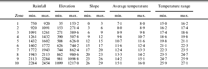
Ten equal-sized intervals of values were defined for each physical environment factor based on the maximum and minimum values of each factor in each spatial unit. The number of intervals was determined based on the interval size that proved most suitable for this dataset in preliminary tests. By using fewer intervals, some situations would be masked, and using more intervals would require a more complex process that would not provide additional, relevant information. Hence, the region was divided into 10 spatial units that were homogeneous for each environmental factor. Such a division into 10 levels, independent for each factor, was exclusive of the analysis described in this section. The spatial units thus defined will be referred to hereinafter as ‘zones’.

Two farm variables were used in the analysis: area under the crop considered (A Crp) and herd size (S Hrd). The first variable (A Crp) is common to all agricultural activities, whereas the second variable (S Hrd) is common to farming activities.

The value assigned to the farm variables was determined for each zone. Given that there was not a proportion between the number of farms and the size of spatial units, the values assigned to farms were standardized by considering the UAA of each farm, in order to obtain comparable results. Results were obtained from eqns (1) and (2), where C _i is the weighting factor, UAA_Ri is the sum of UAA for interval Ri, and Value is the value assigned to the variable considered (A Crp, S Hrd and A Crp).

(1)

$C_{\rm i} \equals {{{\rm Max}.\left( {\sum {\rm SAU}_{{\rm Ri}} } \right)} \over {\sum {\rm SAU}_{{\rm Ri}} }}$

(2)

${{\rm Value} \equals {{{\rm 100} \cdot C_{\rm i}\cdot {\rm Variable}} \over {{\rm Max}{\rm.}\left( {C_{\rm i}\cdot {\rm Variable}} \right)}}}$

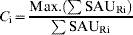
The results of both equations were a dimensionless value that was indicative of the relevance of the farm variable analysed with regard to the physical environment factor considered in the comparison. In order to systematize the process, the analyses were performed by using spreadsheets and the results were represented through bar charts that facilitated the interpretation of results.

Relationship between farming activity and physical environment

As suggested above, the working hypothesis is that there is a relationship between farm location and physical environment factors. Under this assumption, the relationships between different farm variables and physical environment factors are defined in this section.

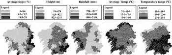
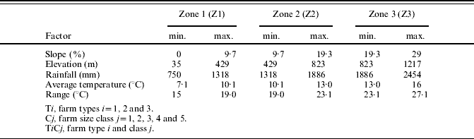
The spatial units (municipalities) with the same interval values for each physical environment factor were organized in groups. Accordingly, three different zones were obtained (Z1, Z2 and Z3), sorted according to minimum, intermediate and maximum values, respectively. The three zones obtained allowed for the division of the territory into distinct areas for each factor (Fig. 1).

Fig. 1.

Spatial zoning of environment factors (average slope, height, rainfall, average temperature, temperature range). Maps show distribution of factors classified in equal intervals as shown in the legend.

All the municipalities (minimum spatial units) showing values of the physical environment factor considered within a preset interval were grouped together. The intervals were equal-sized and independent of the intervals defined in the previous analysis. The number of intervals depended mainly on the influence of the factor considered on the farming activity.

However, before analysing the relationship between physical environment factors and farms, it was considered convenient to confirm whether the distribution of the farm population studied fitted a given theoretical distribution (uniform, Poisson, exponential or normal). Common non-parametric tests such as the chi-square test (Snedecor & Cochran Reference Snedecor and Cochran1989), and the one-sample Kolmogorov–Smirnov (K–S) test (Kolmogorov Reference Kolmogorov1956), were used. After having obtained the empirical and theoretical distributions, the K-S statistic was calculated from the largest difference Di between F(Xi) and F₀(Xi).

The analysis of the distribution of farms builds on the spatial zoning obtained for each factor (Z1, Z2 and Z3). However, the municipalities were grouped based on the overlay of each zone for the various environmental factors (layer overlay). Accordingly, the distribution of the various farm types across 42 spatial units was analysed, which resulted from grouping together the spatial units (municipalities) that belonged to the same interval of values for the physical environment factors considered as a whole.

Following the statistical verification, the relationship between farming activity and physical environment factors was analysed from two different perspectives: (1) considering the degree of adjustment of the production systems to physical environment constraints, and (2) considering the degree of affinity between farm variables and physical environment factors.

The whole process was applied to dairy farms in Galicia, building on previous research works by the authors (Riveiro Reference Riveiro2007; Riveiro et al. Reference Riveiro, Marey, Marco and Álvarez2008), who identified five farm size classes and three farm types: Type 1 (T1), Type 2 (T2) and Type 3 (T3), based on the characteristics of the production system used on the farm. T1 comprised 6094 farms that included silage maize but did not include beef cattle. T2 comprised 8910 farms that did not include silage maize or beef cattle. Finally, T3 comprised 1441 farms with a beef cattle breeding stock of five or more animals, irrespective of the presence of forage crops. (Beef production is included because it is a complementary activity in some dairy farms). Five size classes were identified for each farm type (C1, 10–24; C2, 25–39; C3, 40–54; C4, 55–69 and C5, >69 dairy cows).

By defining different farm types and classes, a greater level of detail was achieved in the analysis because of the availability of different aggregation levels for each land use or activity.

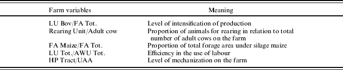
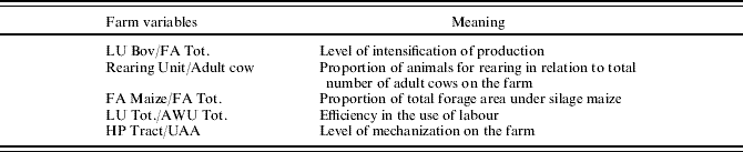
Consequently, the procedure applied to dairy farms included four farm stratification levels for each distinct zone: (a) the set of farms located in the zone, (b) the set of farms belonging to one farm type, (c) the set of farms belonging to a size class and (d) the subset of farms belonging to each farm type and included in a given size class. Based on these basic stratification levels, the farm variables summarized in Table 1 were analysed as indicators of the most relevant features of the production systems used on the farms.

Table 1.

Farm variables analysed as indicators of some characteristics of production systems

Degree of adjustment of production systems to physical environment constraints

The analysis of the relationship between farm variables and physical environment factors provides an explanation for the differences found in the spatial location of farms. Thus, the mean and standard deviation (s.d.) was determined for each of the variables included in Table 1 and each of the three zones defined for each environmental factor. The mean and s.d. of each variable were determined for the different stratification levels, considering the set of farms that corresponded to each level. In order to systematize the process, the analysis was performed by using spreadsheets.

Degree of affinity between farm variables and physical environment factors

This analysis was aimed at finding the environmental characteristics that were most closely related to the farm variables summarized in Table 1. Initially, the mean values of the farm variables, computed according to the method described in the preceding section for the minimum spatial unit, were considered. Such values were grouped into three levels by defining equal-sized intervals between the maximum and minimum values of each variable. The variables were classified again into discrete values designated as low (L), medium (M) and high (H). Then, the mode was determined by quantifying the number of minimum spatial units in which a discrete value (L, M or H) was repeated for each zone (Z1, Z2 or Z3) and each physical environment factor. The mean value of the farm variables was calculated for each of the classes defined according to the mode and for each zone by considering the farms that corresponded to each discrete value L, M and H.

The farm characteristics most closely related to each of the spaces derived from the zoning proposal were determined based on the physical environment factors considered. As in previous analyses, spreadsheet-based tools were used to make the process more systematic.

RESULTS

Analysis of spatial distribution

The analysis of spatial distribution was performed for different land uses or farming activities. In order to illustrate the methodology described in this paper, three representative land uses were chosen: (a) wheat, (b) rainfed potato and (c) dairy cattle farming on Type 1 farms.

Wheat

The analysis included 1631 Galician farms with at least 1 ha of land used to grow wheat and registered in the 1999 Agricultural Census (INE 1999). Smaller farms were not considered because such farms were not exploited for commercial purposes and consequently did not use mechanized production systems. The farm variable selected for analysis was the area under wheat, which was the variable that best illustrated the extent of the crop area.

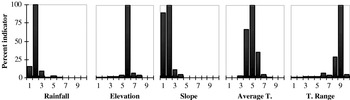
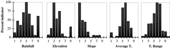
The analysis of results revealed that the main constraints were terrain slope and plot size, which considerably reduced the UAA used for growing wheat in Galicia. As shown in Fig. 2, most of the area under cultivation was concentrated in land areas with slopes below 6% (intervals 1 and 2). Furthermore, the climatic conditions in the region were not the most suitable for growing cereals, as suggested by the graphs in Fig. 2. In general, the primary location of wheat was associated with very small intervals of values for all the environmental factors considered (Fig. 2). Actually, wheat has been gradually replaced by more profitable crops. The low profitability of wheat stems from environmental constraints that reduce the profitability of the crop because of increased cultivation costs, thus reducing market competitiveness.

Fig. 2.

Indicator of the distribution of number of rainfed wheat farms (standardized by the Utilized Agricultural Area of each municipality) in ten equal intervals for each envirnomental factor.

Potato

Potato cultivation is widespread in the region as a rainfed crop for home-consumption, but fewer areas are used to cultivate potato for commercial purposes. In the current paper, 1271 farms with an individual crop area equal to or above 0·4 ha and registered in the 1999 Agricultural Census were considered (INE 1999). A crop area equal to or above 0·4 ha was considered to exceed the limit for home-consumption (EIDO-USC 2004).

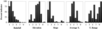
Because commercial potato crop production requires mechanization, both terrain slope and plot size are constraints that limit the UAA used for growing potato. As shown in the graphs in Fig. 3, the potato crop was present in locations with wider intervals of values of the physical environment variables considered. Moreover, the graphs evidenced two parallel realities: (1) the presence of farms specialized in the potato crop, which were located in particular spaces, and (2) a large number of farms that commercialized potato as a complementary activity, which required lower mechanization levels. Lower mechanization levels involve fewer environmental requirements and allow for the presence of steeper slopes.

Fig. 3.

Indicator of the distribution of number of rainfed potato farms (standardized by the Utilized Agricultural Area of each municipality) in ten equal intervals for each envirnomental factor.

Dairy cattle farming

In the current study, the 16 445 Galician farms with at least 10 dairy cows were chosen. By way of example, this section presents the results obtained for the 6094 farms included in T1 (according to the farm types described in preceding sections), which is the most common farm type at present.

Production systems were initially adjusted to topographical and structural constraints, which resulted in a large number of small family farms scattered over the region. Such constraints have been solved over time, and now the number of farms is smaller. Still, most Galician farms are family run, but they are larger in size and use professional production systems. In addition, the requirements of the new production systems have restricted the continuity of farms with regard to their spatial location.

The results shown in Fig. 4 were in agreement with the situation depicted in the preceding paragraphs. In Fig. 4, wide intervals of values of the physical environment factors were considered suitable. The only zones that were excluded were zones with very low average temperatures and steep average slopes that were not suitable for silage maize, which is the feed base on such farms.

Fig. 4.

Indicator of the distribution of number of T1 dairy farms (standardized by the Utilized Agricultural Area of each municipality) in ten equal intervals for each envirnomental factor.

As compared to the information reported by Bouhier (Reference Bouhier2001) for the period 1950–70, the results presented above evidenced the trend of change in the agricultural sector with regard to the spatial distribution of farms in relation to physical environment factors.

Relationship between farming activity and physical environment

The results of the statistical test performed to verify whether the distribution of the farm population studied fits a given theoretical distribution reveals that the distribution of the farm population does not fit any of the types of distribution tested (uniform, Poisson, exponential or normal; because most of the values obtained are P<0·001. All the values are 0·000 except four, of which two are lower than and the other two 1·000 and 0·245, correspond to non-representative samples of 7 and 18 farms, respectively. Moreover, the results justify the need to use the analysis method described earlier.

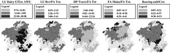
Figure 5 shows the result of having calculated the mean of the values of the farm variables considered for each spatial unit (municipalities) graphically, by separating the values obtained into three intervals based on the maximum and minimum values. The maps show very homogeneous zones. The homogeneity of the results summarized in Fig. 5 and the results presented earlier confirm that there is a relationship between the production systems used on the farms and physical environment factors.

Fig. 5.

Spatial distribution of farms included in group T1C2 based on values of process variables, classified in equal intervals as shown in the legend.

After having confirmed the presence of a relationship between the production systems used and physical environment factors, which farm variables had the strongest influence and the extent of the influence were determined. Knowing the extent of the influence of the farm variables considered provides information about which are the most suitable production systems for each zone and about optimization possibilities, and is useful in the context of agricultural production planning.

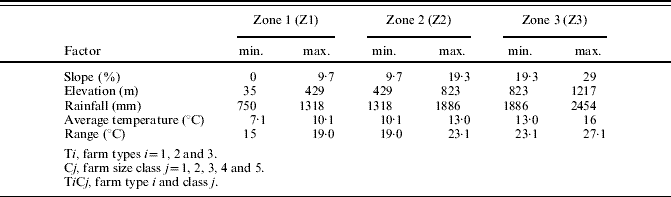
The results for dairy farming are shown according to the following structure: the first section presents the results of the analysis of the degree of adjustment of production systems to physical environment constraints, and the second section presents the results of the analysis of the degree of affinity between farm variables and physical environment factors. Interpretation of the results is made according to the values presented in Table 2.

Table 2.

Caption for the interpretation of Tables 3–8

Degree of adjustment of production systems to physical environment constraints

The analysis was performed using the methodology defined earlier for the four farm stratification levels in each distinct zone. This section presents the results for the five variables considered and some possible scenarios.

(A) Variable Horse Power Tractor/Utilized Agricultural Area (HP Tract/UAA)

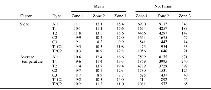
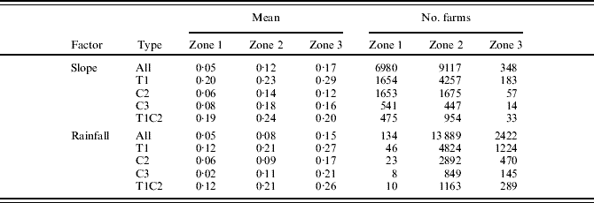
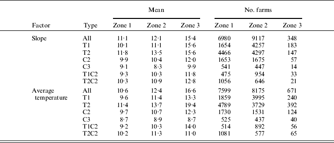
This variable is used as an indicator of the mechanization level on farms. Table 3 shows the values of slope and average temperature for the different stratification levels of the variable HP Tract/UAA. Results confirmed that the increase in terrain slope and in average temperature (greater need for tilling and greater suitability for crop growth) involved an increase in the mechanization level of farms. As compared to the overall mean, T1 farms showed lower values and T2 showed higher values. Such a result was reversed for the factor ‘slope’ in Z3, which showed values that were slightly higher than the mean, probably because of the presence of a higher percentage of small farms.

Table 3.

General differentiation among zones for the variable Horse Power Tractor/Utilized Agricultural Area

Full details of farm class and size are given in Table 2.

By comparing the results obtained for farms included in class C2 with the results obtained for farms included in class C3, it was observed that larger farms showed lower mechanization levels and that the differences among zones became smaller with the increase in farm size. Moreover, the results obtained for farms included in classes C2 and C3 were quite similar for both factors, which suggests that the variable HP Tract/UAA depended on the production systems used on the farms rather than on farm zoning based on physical environment factors.

(B) Variable Forage Area Maize/Forage Area Total (FA Maize/FA Tot.)

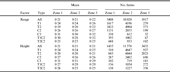
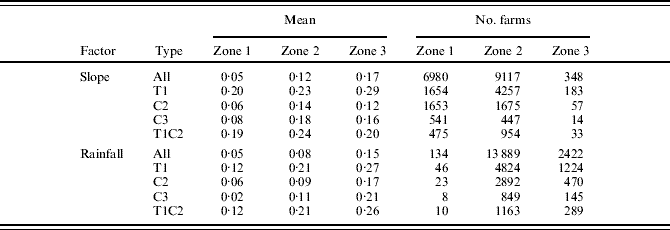
Table 4 shows the values of slope and average temperature for different stratification levels of the variable FA Maize/FA Tot. Because the maize crop was exclusive to farms included in T1, the results obtained for other farms were included in the table.

Table 4.

General differentiation among zones for the variable Forage Area Maize/Forage Area Total

Full details of farm class and size are given in Table 2.

Contrary to expectations, the proportion of UAA used for growing maize increased with the increase in slope (with an increase in Z3), which did not mean that the cropped area of maize was larger. The results for the farms included in T1C2 contradicted this trend, with a larger maize crop area in zones with average slope values (Z2). These results suggest that zone Z3 comprised a larger proportion of small farms with less demanding harvesting systems in terms of slope. Contrary to expectation, the areas with the gentlest slopes did not correspond to the greatest areas of crops which could be related to the increased liability of flatter areas to become flooded, making seeding and harvesting difficult.

With regard to rainfall, the relative maize crop area on farms increased with the increase in rainfall levels for the set of farms included in type T1 and particularly for farms included in size class C2. The high crop water requirements of maize would justify a lower presence of the maize crop in zone Z1. However, although the rainfall levels in the region are not too high during the crop cycle (May–September), the lower presence of maize in zone Z1 could be related to the preference for steep average slopes, which are more easily drained.

Finally, on average, the presence of maize in classes C2 and C3 or in the whole sample of farms was very low (0·02–0·08) because the number of farms included in farm type T1 was much lower than the number of farms included in T2.

The genetic improvement of dairy cattle has increased milk yield per cow and gradually reduced the productive life of cows, thus increasing the replacement rate (Africor Lugo 2007). The use of the variable Rearing Unit/Adult cow allowed determination of whether the effects of genetic improvement affected the whole territory and all the production systems to the same extent. The results in Table 5 demonstrate the irrelevance of farm zoning based on physical environment factors. Results were similar among zones for the same farm stratification level, both for the factors presented in the table and for the rest of factors considered. Differences, which were hardly significant, occurred only among stratification levels, i.e. among different farm sizes or farm types.

Table 5.

General differentiation among zones for the variable Rearing Unit/Adult cow

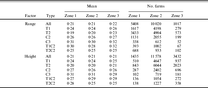
Full details of farm class and size are given in Table 2.

(D) Variable Livestock Units Dairy Cow/Forage Area Total (LU Dairy C./FA Tot.)

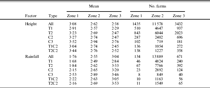
This variable is used as an indicator of stocking density and consequently, of the level of intensification of farms. Table 6 shows disparate results for different farm stratification levels and zones with different heights above sea level (coast and mountain) or different rainfall levels. Stocking density was lower in high zones (mainly in mountain areas) than near the coast. This might reflect the higher natural productivity of coastal areas. Similarly for rainfall, the highest stocking densities were observed in zones with the highest rainfall levels, which was in agreement with the production potential of the different zones. Nevertheless, there were substantial differences in the stocking densities of some farm stratification levels.

Table 6.

General differentiation among zones for the variable Livestock Units Dairy Cow/Forage Area Total

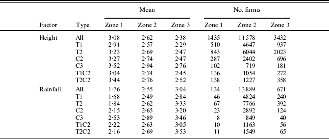
Full details of farm class and size are given in Table 2.

The results, obtained by considering different levels of aggregation in the analysis of data, suggested that the heterogeneity of the production systems used on dairy cattle farms was largely caused by the adjustment of the production systems to the conditions and constraints of the environment where the activity was carried out.

(E) Variable Total Livestock Units/Total Annual Working Units (LU Tot./AWU Tot.)

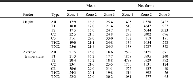
This variable is taken as an indicator of the level of efficiency of the use of farm labour. Some authors have suggested that efficiency is achieved mainly by the planning of the different farm activities. This statement can be true for farms that are similar in all their characteristics. However, the statement is not valid for farms with different characteristics. The results summarized in Table 7 showed substantial differences in efficiency, both for farms belonging to the same farm type or size class and for farms belonging to different farm types or size classes but located in the same zone.

Table 7.

General differentiation among zones for the variable Livestock Units Total/Annual Working Units Total

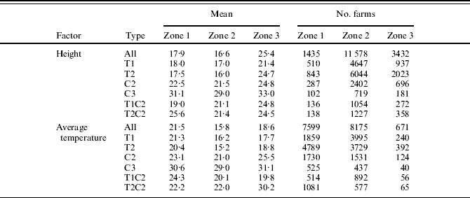
Except for some particular cases, efficiency appeared to be lower in the zones where most farms were concentrated, which corresponded to zones with average values of height above sea level and temperature. For height above sea level, the highest efficiency values corresponded to the highest locations regardless of farm stratification level. Such results could be related to less intense forage crop production, lower stocking densities and more intense grazing.

The trend was less clear for average temperature. When farms belonging to all size classes were considered (All, T1 and T2), the highest efficiency values were observed in zones with low average temperature values (e.g. mountain areas). However, when larger farms were considered (C2, C3 and T2-C2), efficiency was higher in zones with the highest average temperatures (zones near the coast).

When both factors were considered jointly, the largest farms, with higher stocking densities, showed the highest efficiency values and corresponded to the zones that were most suitable for forage crop production. Conversely, smaller farms showed lower efficiency values, but efficiency was higher in mountain zones or in zones with more extensive production systems.

Degree of affinity between farm variables and physical environment factors

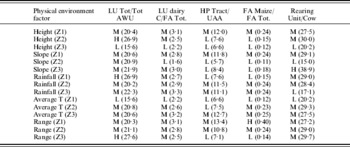
Three farm types and five size classes (a total of 15 farm groups) were defined for dairy cattle farms. For each group, five variables were analysed and contrasted considering the three zones defined for each of the five physical environment factors. Therefore, 1125 results were possible. Table 8 and shows the 75 results obtained for the stratification level that comprised the farms belonging to T1 and size class 2 (C2).

Table 8.

An example of mode categories and mean values for variable/factor pairs on T1C2 farms

* Legend for mode categories: L (low), M (medium), H (high) (see also Fig. 6).

Table 9.

A caption for the interpretation of Figs 2–4

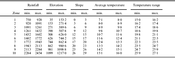
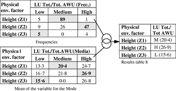
Figure 6 shows how the results were structured, thus facilitating the interpretation of Table 8. The frequencies of each of the three zones (Z1, Z2 or Z3) for a given environmental factor were determined for each variable, which allowed determination of the Mode for the farm variable considered and for each zone (Z1, Z2 and Z3). In the example included in Fig. 6, the frequencies 89, 47 and 5 corresponded to modes M, H and L for the variable LU Tot./AWU Tot. in zones Z1, Z2 and Z3 when the factor ‘height above sea level’ was considered. Just below the frequencies, Fig. 6 shows the mean of farms included in each modal class for each variable. In the example, the following values of LU Tot./AWU Tot., 20·39, 26·90 and 15·60, were the means for modal classes M, H and L. Both results are summarized in Table 8 under the heading ‘Mode (value of the mean)’. In the example presented in Fig. 6 for zone Z2 and height above sea level, the modal class of the variable LU Tot./AWU Tot. was H and the value of the mean was 26·90.

Fig. 6.

Example of mode and mean for variable/factor pairs on T1C2 farms for interpretation of Table 8.

The results were aimed at determining reference values for different analysis procedures (technical–economical and financial analysis, analysis of possible alternatives, location optimization, etc.) used in agricultural production planning processes.

Some specific observations can be made on the results obtained for farm group T1C2 (Table 8). For the variable LU Tot./AWU Tot., the prevailing modal class was M (intermediate values of the variable), with values ranging from 20·15 to 22·27. Because this variable was used as an indicator of the efficiency of use of farm labour, the most frequent efficiency values on farms were intermediate values. Apparently, low efficiency values (L) corresponded to high zones with low average temperatures, i.e. mountain areas. Conversely, the highest efficiency values (H) corresponded to very specific inland zones with average height values, low rainfall levels and high temperature ranges.

For the variable Livestock Units Bov/Forage Area Total (LU Bov/FA Tot.), an indicator of stocking density), the prevailing modal class was M, with values ranging from 2·47 to 3·32. High values did not prevail in any of the zones and low values prevailed in high zones with average mean slopes and low average temperatures, which corresponded to very specific inland zones of the region.

With regard to HP Tract/UAA, a variable used as an indicator of the level of mechanization on farms, the prevailing modal classes were M and L. Modal class M (intermediate values) prevailed in low zones with mild slopes, average or high rainfall levels, high average temperatures and low or intermediate temperature ranges, common in zones near the coast and adjacent inland plains. These zones are most suitable for forage crop production and show the highest level of intensification of dairy cattle farms. In the rest of the zones, and mainly in inland mountain zones, the prevailing modal class was L (low mechanization levels), coinciding with a lower suitability for forage crop production and a lower intensification on farms.

For the variable FA Maize/FA Tot. (used as an indicator of the extent of forage maize production), the prevailing modal classes were M and L, coinciding with the zones where M and L were the prevailing modal classes for the variable used as an indicator of the level of mechanization on farms (HP Tract/UAA), i.e. forage maize was more present in zones near the coast and relatively less present in inland zones. High values of FA Maize/FA Tot. (modal class H) were observed only in zones with small temperature ranges, i.e. in coastal areas.

Finally, modal class M (intermediate values of the variable) prevailed for the variable used as an indicator of the number of rearing units on farms (Rearing unit/Adult cow), with values in the range 0·27–0·30. The lowest numbers (L modal class) were observed in very specific mountain zones, probably coinciding with less intensive farming and, consequently, with a longer productive life of cows. Modal class H (high rearing unit values) corresponded to zones with steep slopes, which appeared to contradict the rest of the results. This was due to the fact that the value occurred only in a minimum spatial unit and was obtained from a very small farm sample, which suggests that this value was not representative of the values obtained for the variable.

DISCUSSION

European Commission Decision 85/377/EEC establishes a typology for agricultural holdings based on the main activities providing the highest share of farm income. This typology enables comparisons of farm activities among member states for different periods. Andersen et al. (Reference Andersen, Elbersen, Godeschalkc and Verhoog2007) suggested extending the EU farm typology by further classifying the farms according to environmental criteria, and considered a combination of two dimensions: land use and intensity in terms of (financial) output per hectare (low, medium and high intensity). After having analysed a number of crops and dairy cattle farms for the different EU-15 regions, Andersen et al. (Reference Andersen, Elbersen, Godeschalkc and Verhoog2007) observed a relevant difference in the distribution of all the types of farms at the regional level and large differences in the environmental characteristics of farms.

Whereas the proposal by Andersen (et al. Reference Andersen, Elbersen, Godeschalkc and Verhoog2007) is suitable for a regional analysis, the methodology presented in the current paper has been developed for smaller areas, taking the municipality as spatial unit. The municipality is the lowest level of aggregation allowed by the microdata from Agricultural Censuses in Spain. More specifically, the results obtained for dairy farms in Galicia reveal important differences in the spatial distribution of the different groups of farms, which suggests that farm location is related to physical environment factors. However, as expected, this relationship does not fit any theoretical distribution function.

In addition, the present results reveal that the current methodology is suitable for the assessment of the environmental behaviour of farms insofar as the analysed farms show, right from the outset and depending on the crop considered: (a) different degrees of correlation between the location of farms and the different environmental factors, (b) different characteristics of the production systems associated with homogeneous spaces for each environmental factor and (c) different degrees of affinity in the relationships between single variables of the production process and environmental factors. This is very interesting and useful in decision-making for the implementation of some agricultural and environmental policies.

The methodology described in the current paper allows an estimation of the value of the variables used as indicators in different locations associated with specific values of the environmental factors considered. For example, stocking density values (LU Bov/FA Tot.) are higher in zones with higher rainfall values and lower in the zones with the highest elevations (Table 8). The values obtained for the relationship between FA Maize/FA Tot. and HP Tract/UAA as indicators of tillage intensity are higher in zones with very gentle slopes and average to low rainfall levels. Consequently, the most aggressive tillage operations are observed in less sensitive zones.

The traditional Galician landscape, associated with a high degree of land fragmentation, has been and still is subjected to profound transformations derived from the implementation of new production systems. Frequently, the environment has been adapted to the production system, particularly through land consolidation actions. However, the convenience of adapting some production systems to the physical environment is questionable, particularly in some spaces.

The methodology of analysis proposed here, when considering all the land uses present in the region and other physical environment factors and farm variables, would enable a better knowledge of the activity–environment relationship because of the interaction between land use and landscape structure. Similar conclusions were drawn by Thenail & Baudry (Reference Thenail and Baudry2004) from a study conducted in a French region with high dairy production.

A study carried out by Kristensen et al. (Reference Kristensen, Thenail and Kristensen2004) analysed the relationship between the characteristics of farms and landscape changes by interviewing 160 farmers, and identified the farm characteristics that most affected landscape changes. The present work, based on data from the 1999 Agricultural Census does not include a temporal approach. However, the methodology proposed in this paper could be used to perform similar analyses by comparing municipal data from the 1999 Census, the 1989 Agricultural Census and the future 2009 Agricultural Census. Moreover, the whole population of farms could be considered in such analyses.

Finally, Thenail (Reference Thenail2002) studied the relationships between farm characteristics and the variation in the density of hedgerows in a region of Brittany, France. If the specific location of each farm within a limited space could be known from data provided by agricultural censuses, new variables could be introduced in the analysis by using field information or data obtained from other sources, and a higher level of specification could be achieved, particularly in terms of environmental and landscape aspects.

CONCLUSIONS

The main conclusions to be drawn are that the analysis method presented in the current study allowed the identification of individual relationships between farm variables and physical environment factors, which usually explain associations between production systems and the environment in which they were developed. The usefulness of the method can also be extended to determine the effects of changes in production systems on the environment, measure their sustainability, define the most suitable production systems for each location and/or strategically assess the introduction of new farms. Additional relevance can be found in its data source, which can be compared with others at the European level, and the availability of data, which avoids the need for costly sampling processes. Nevertheless, despite the potential of the method, limitations derived from data aggregation reveal the need for smaller or more homogeneous spatial units in any future census.

The authors are grateful to the Galician government, Xunta de Galicia, Dirección Xeral de Investigación, Desenvolvemento e Innovación, for funding the project PGIDIT06RAG29101PR and to the Spanish Ministry of Education and Science for funding the project AGL2006-04789/AGR.

References

REFERENCES

Africor Lugo (2007). Memoria de Actividades da Asociación Provincial de Criadores de Frisón de Lugo para o Control de Rendementos. Available online at http://www.africorlugo.com/memorias.asp (verified 16 July 2009).Google Scholar

Andersen, E., Elbersen, B., Godeschalkc, F. & Verhoog, D. (2007). Farm management indicators and farm typologies as a basis for assessments in a changing policy environment. Journal of Environmental Management 82, 353–362.Google Scholar

Bennett, S. J. & Galwey, N. W. (2002). The use of spatial analysis to measure the effect of environmental heterogeneity on genetic variation in Trifolium species from Sardinia. Journal of Agricultural Science, Cambridge 139, 283–294.Google Scholar

Bouhier, A. (2001). Galicia. Ensaio Xeográfico de Análise e Interpretación dun Vello Complexo Agrario. Tomos I y II (Translated by B. Casal Vila). Santiago de Compostela, Spain: Xunta de Galicia – Consellería de Agricultura, Gandería e Montes. Caixanova.Google Scholar

Brasier, K. J. (2005). Spatial analysis of changes in the number of farms during the farm crisis. Rural Sociology 70, 540–560.CrossRef Google Scholar

Deffontaines, J. P., Thenail, C. & Baudry, J. (1995). Agricultural systems and landscape patterns – how can we build a relationship? Landscape and Urban Planning 31, 3–10.CrossRef Google Scholar

De Miguel, J. C., Perez, T. & Rodríguez, X. A. (2002). Tendencias productivas en las explotaciones de leche gallegas. Revista Galega de Economía 12, 1–18.Google Scholar

Dendoncker, N., Rounsevell, M. & Bogaert, P. (2007). Spatial analysis and modelling of land use distributions in Belgium. Computers Environment and Urban Systems 31, 188–205.CrossRef Google Scholar

EIDO-USC (2004). Estudios Comarcales De Ordenación Productiva Agraria De 21 Comarcas. Santiago De Compostela, Spain: Xunta De Galicia – Consellería De Política Agroalimentaria e Desarrollo Rural.Google Scholar

Hodson, D. P. & White, J. W. (2007). Use of spatial analyses for global characterization of wheat-based production systems. Journal of Agricultural Science, Cambridge 145, 115–125.Google Scholar

IGE (2006) Galicia en Cifras. Available online at http://www.ige.eu/estatico/html/gl/galicia_en_cifras/galicia_2006/gcifras_2006_c07.pdf (verified 16 July 2009).Google Scholar

INE (1962). Censo Agrario de 1962. Madrid, Spain: Instituto Nacional de Estadística.Google Scholar

INE (1989) Base de microdatos del Censo Agrario de 1989. Available online at http://www.ine.es/prodyser/micro_censoag.htm (verified 16 July 2009).Google Scholar

INE (1999) Base de microdatos del Censo Agrario de 1999. Available online at http://www.ine.es/prodyser/micro_censoag.htm (verified 16 July 2009).Google Scholar

INE-EEEA (2003) Encuesta sobre la Estructura de las Explotaciones Agrícolas de 2003. Available online at http://www.ine.es/proyectos/exploagri/proy_explo_agri.pdf (verified 19 July 2009).Google Scholar

INE-EPA (2003) Encuesta de Población Activa. Año 2003. Available online at http://www.ine.es/jaxi/menu.do?type=pcaxis&path=/t22/e308_mnu&file=inebase&N=&L=0 (verified 16 July 2009).Google Scholar

Jongman, R. H. G. (2002). Homogenisation and fragmentation of the European landscape: ecological consequences and solutions. Landscape and Urban Planning 58, 211–221.CrossRef Google Scholar

Kolmogorov, A. (1956). Foundations of the Theory of Probability, 2nd edn.New York: Chelsea Publishing Company.Google Scholar

Kristensen, L. S., Thenail, C. & Kristensen, S. P. (2004). Landscape changes in agrarian landscapes in the 1990s: the interaction between farmers and the farmed landscape. A case study from Jutland, Denmark. Journal of Environmental Management 71, 231–244.CrossRef Google Scholar PubMed

López Iglesias, E. (2000). O sector agrário galego ás portas do século XXI: balance das suas transformacións recentes. Revista Galega de Economía 9, 167–196.Google Scholar

MAPA (2004). Sistema de Información Geográfica de Datos Agrarios (SIGA). Available online at http://www.mapa.es/es/sig/pags/siga/intro.htm (verified 16 July 2009).Google Scholar

Mignolet, C., Schott, C. & Benoît, M. (2004). Spatial dynamics of agricultural practices on a basin territory: a retrospective study to implement models simulating nitrate flow. The case of the Seine basin. Agronomie 24, 219–236.Google Scholar

Mignolet, C., Schott, C. & Benoît, M. (2007). Spatial dynamics of farming practices in the Seine basin: Methods for agronomic approaches on a regional scale. Science of the Total Environment 375, 13–32.Google Scholar

Riveiro, J. A. (2007). La tipificación y clasificación de explotaciones como una herramienta para diferenciar los distintos sistemas productivos – Aplicación a las explotaciones de vacuno lechero en Galicia. PhD thesis, Universidad de Santiago de Compostela, Santiago, Spain.Google Scholar

Riveiro, J. A., Marey, M. F., Marco, J. L. & Álvarez, C. J. (2008). Procedure for the classification and characterization of farms for agricultural production planning: application in the Northwest of Spain. Computers and Electronics in Agriculture 61, 169–178.Google Scholar

Rodríguez-Couso, M., Teijido, M., Álvarez, C. J. (2006). Rural development in Galicia (north-west Spain). Outlook on Agriculture 35, 183–189.CrossRef Google Scholar

Roschewitz, I., Thies, C. & Tscharntke, T. (2004). Are landscape complexity and farm specialisation related to land-use intensity of annual crop fields? Agriculture, Ecosystems and Environment 105, 87–99.CrossRef Google Scholar

Schmit, C. & Rounsevell, M. D. A. (2006). Are agricultural land use patterns influenced by farmer imitation? Agriculture, Ecosystems & Environment 115, 113–127.CrossRef Google Scholar

Sineiro, F. (2006). A evolución socioeconómica dos sectores rurais galegos. Recursos Rurais – Serie Cursos 4, 47–55.Google Scholar

Skop, E. & Schou, J. S. (1999). Modeling the effects of agricultural production. An integrated economic and environmental analysis using farm account statistics and GIS. Ecological Economics, 29, 427–442.CrossRef Google Scholar

Snedecor, G. W. & Cochran, W. G. (1989). Statistical Methods. 8th edn.Ames, IA: Iowa State University Press.Google Scholar

Thenail, C. (2002). Relationships between farm characteristics and the variation of the density of hedgerows at the level of a micro-region of bocage landscape. Study case in Brittany, France. Agricultural Systems 71, 207–230.Google Scholar

Thenail, C. & Baudry, J. (2004). Variation of farm spatial land use pattern according to the structure of the hedgerow network (bocage) landscape: a case study in northeast Brittany. Agriculture, Ecosystems and Environment 101, 53–72.CrossRef Google Scholar

Vence, X. (2000). Cambio estrutural e innovación na economía galega. Os retos na soleira do século XXI. Revista Galega de Economía 9, 43–88.Google Scholar

Winkler Stirm, J. E. & St-Pierre, N. R. (2003). Identification and characterization of location decision factors for relocating dairy farms. Journal of Dairy Science 86, 3473–3487.Google Scholar

Xunta de Galicia. (2007) Consellería de Medio rural. Available online at http://mediorural.xunta.es/nc/areas/infraestruturas/concentracions_parcelarias/buscador/ (verified 16 July 2009).Google Scholar

Zhu, J. & Morgan, G. D. (2004). Comparison of spatial variables over subregions using a block bootstrap. Journal of Agricultural, Biological and Environmental Statistics 9, 91–104.CrossRef Google Scholar

Fig. 1.Spatial zoning of environment factors (average slope, height, rainfall, average temperature, temperature range). Maps show distribution of factors classified in equal intervals as shown in the legend.

Table 1.Farm variables analysed as indicators of some characteristics of production systems

Fig. 2.Indicator of the distribution of number of rainfed wheat farms (standardized by the Utilized Agricultural Area of each municipality) in ten equal intervals for each envirnomental factor.

Fig. 3.Indicator of the distribution of number of rainfed potato farms (standardized by the Utilized Agricultural Area of each municipality) in ten equal intervals for each envirnomental factor.

Fig. 4.Indicator of the distribution of number of T1 dairy farms (standardized by the Utilized Agricultural Area of each municipality) in ten equal intervals for each envirnomental factor.

Fig. 5.Spatial distribution of farms included in group T1C2 based on values of process variables, classified in equal intervals as shown in the legend.