Comparative Enrollment Statistics

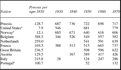
The claim that by the mid-nineteenth century American youth had become the most educated in the world rests largely on comparative enrollment statistics. National offices of education release these reports and researchers calculate rates by dividing the children enrolled by the total population or school age population, most often 5 through 19 or 5 through 14 (Easterlin Reference Easterlin1981; Flora et al. Reference Flora1983). Few polities, however, possessed such offices circa 1850, so scholars have to make estimates from very incomplete data. One of the most comprehensive compilations can be found in Lindert (Reference Lindert2004). Table 1 displays the ratio of students enrolled in school to children in the population ages 5 through 14 for those countries in Lindert's list that had results for 1850.

TABLE 1.

Students enrolled in primary schools, per 1,000 children of ages 5–14 1830–70

Source: Lindert Reference Lindert2004: 91–93, table 5.1; McEvedy and Jones Reference McEvedy and Jones1978 .

^a Public school students only.

At first glance the United States does quite well, coming in ahead of almost every country except Prussia, the paragon of regularized schooling during the period. The density measure I added renders the performance even more impressive. A major barrier in educating children in predominantly rural societies was allegedly the distance they had to travel and the costs of erecting schools in communities with a small population base. All the European nations had density levels more than 100 persons per square mile save Norway, and in that case the low number is deceptive because almost all of that country's inhabitants clustered within the far southern portion of the country.

A closer look at the data, however, raises doubts over how seriously to take differences in the statistics between the United States and other North Atlantic countries. First of all, the source for the United States’ 1830 and 1850 numbers are “guesses repeated in many sources.”Footnote ¹ Second, while the 1870 enrollment rate of 77.9 percent is based on an actual Education Office report on numbers enrolled, when divided by the population ages 5 through 14 the results can be misleading. The enrollees in this period are of all ages: thus the enrollment numerator includes students excluded in the denominator.

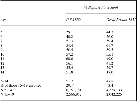
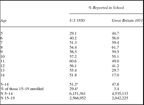
To understand why this situation might especially inflate US numbers, it is necessary to turn to another mid-century source available for the United States that contains age-specific enrollment information—the public use sample of the 1850 decennial population census. It just so happens that an 1851 public use sample with the same kind of information by age exists for Great Britain, enabling a comparison. Table 2 displays the proportion of US children ages 5 through 14 in 1850 noted as being in school with the percentage labeled as “scholars” in Britain in 1851. As all classes of Britons were being counted, the US numbers must incorporate enslaved children in the denominator if we are testing who had the edge in providing primary education to their population. As the argument has been that Britain's enrollment rate suffered vis-à-vis America's from its elitist and antidemocratic tendencies, one has to be sure that the advantage is not simply the result of excluding from the calculations the 15 percent of US children who were enslaved, while including the children of the lowest income British families.Footnote ² If only free children in the United States are counted, 60.3 percent were enrolled in school, which contrasts quite favorably with the 47.8 percent of British children reported in school in table 2. However, incorporating the enslaved children brings the US percentage down to the 51.2 percent shown in the table. In addition, definitions of who were to be counted as “in school” appear to have been less stringent in America. To answer positive to a child's school enrollment in the US census, a parent only had to attest to a son or daughter being schooled at least one day during the year, and evening school could be counted. The British parent had to affirm “daily” attendance or regular instruction under a governess or tutor, seemingly a higher standard. A comparison of the responses on the British household census with those on its census of schools (Coleman Reference Coleman and Wrigley1972: 402–3) shows that the latter reported 6 percent fewer students than the former. In America the same comparison finds 10.3 percent fewer.Footnote ³ Such a bias, however, in both cases may be attributable to the absence of private nondenominational primary school reports in the American case and a reputed undercounting of such schools in Britain. In short, the household reporting stands up well in both countries, as apparently at this point relatively little stigma was attached to admitting one's child did not attend school. Forty-nine percent of the children being schooled were female in both of the samples, so differences in gender discrimination do not surface in these statistics. Regional variations affected the results in both nations. As mentioned earlier, enrollments in the South trailed those in the North of the United States, but Britain had its own variations, with Scotland coming in on top, England next, and Wales coming in a very distant third. The effects of region and ethnicity on schooling will be examined in more detail in the following text.

TABLE 2.

Comparison of percentage of children being schooled by age, 1850–51, United States and Great Britain

Source: Ruggles et al. Reference Ruggles2010 and Minnesota Population Center 2010. It is adapted from Schürer, K., and M. Woollard (2008) National Sample from the 1851 Census of Great Britain [computer file]. Colchester Essex, History Data Service, UK Data Archive.

^a US figures adjusted to include enslaved children. See text for the percentage enrolled with enslaved children excluded.

The main contrast disclosed in table 2 involves ages in school. The British packed their elementary schooling into ages 5 through 12, with only 17 percent of 14 year olds enrolled, while the Americans still had more than half in school at that age. Only between ages 6 and 10 were a majority of British youth enrolled in school, while in the United States enrollment peaked at age 11 and a majority registered for some period of time between ages 7 and 14. Officials at the time complained about what they considered the deleterious impact on the class environment of having so many older youth still studying reading and writing (Soltow and Stevens Reference Soltow and Stevens1981: ch. 4), but the degree to which US teens beyond 14 still were enrolling has not been spotlighted nor its effect on international comparisons considered. Table 2 shows that 29.4 percent in the 15 through 19 age category had not exited school, compared to a mere 3.4 percent of their British counterparts. These numbers suggest an important reason for the relatively high US enrollment percentage shown in table 1: many 15 through 19 year olds are being reported in the 5 through 14 age category.

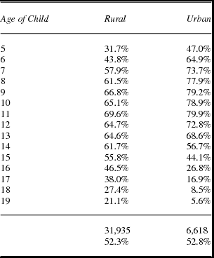
If this late teen enrollment represented greater numbers of students in secondary school, then there would be no problem with equating the higher numbers with more education, but circa 1850 the vast majority of American boys and girls only received instruction in ungraded one-room schools that specialized in the 3Rs. According to Goldin and Katz (Reference Goldin and Katz2008: 188), who have studied high school education the most extensively, as late as 1870 merely 6.5 percent of 15 through 18 year olds were enrolled in a public or private secondary institution. Superannuated common school students, moreover, were much more prevalent in rural America than among the 15 percent of the population that lived in urban areas. Appendix 1 breaks down the enrollment percentages for the free population under 20 by urban and rural residency, revealing that, at age 16, 26.8 percent of urban youth went to school whereas 46.5 percent of their rural counterparts did. At age 19 the percentages were 5.6 percent and 21.1 percent, respectively. Boys, many of whom may have been involved in agricultural labor, predominated over girls in this older age group.

The educational sprawl revealed in the US age-specific enrollment numbers then alerts us to a third problem in making comparisons—enrollments in the nineteenth century do not serve as a good proxy for attendance. Records on actual attendance and school terms in individual schools during the first half of the nineteenth century are rare, and they invariably come from the states Cubberley (Reference Cubberley1934: 97) in his classic study of public education in United States categorized as the “good-school-conditions group”: New England, New York, and Ohio, the latter two being recipients of heavy New England immigration. Average daily class attendance in the few country schools with surviving records ranged from 36 percent to 62 percent days in the session. Terms could last for three to six months with some terms broken into two parts with different attendees (Beadie Reference Beadie2008, 2010; Brooke Reference Brooke2010; Gilmore Reference Gilmore1985; Soltow and Stevens Reference Soltow and Stevens1981). In 1870 when the US Education Office published the first national data, average days of attendance stood at 79.4 per enrolled student or about four months (at 20 days a month), and the average number of days schools remained in session amounted to 132 or about six and a half months. Moreover, because some of the districts with the lowest attendance and duration of school terms failed to report in 1870, the inclusion of them in later decades meant the mean did not rise appreciably until after 1890.Footnote ⁴ For every state that averaged terms of eight months, many more existed that averaged three to five, and not just in the South. Nineteenth-century Americans enrolled in school for such a long period of their youth because they did not go for consecutive years, months, weeks, or days. They frequently absented themselves, and schools did not stay open for that long (Angus et al. Reference Angus, Mirel and Vinovskis1988). Consequently the total number of days attended probably constitutes the best single estimate of the amount of schooling, as it captures both the behavior of children and parents and the constraints imposed by school district terms.

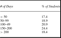
Parliamentary inquiries into “popular” education, meaning that available to the children of those outside of the elites and the urban middle classes, show British students attending more days because school terms lasted longer than in America. The Newcastle Commission Report (Great Britain Parliamentary Papers 1861), issued during a period of Liberal Party rule, tracked the attendance during the 1850s in more than 1,800 English and Welsh public day schools, partially subsidized by government grants. They surveyed schools from all business sectors—agricultural, manufacturing, mining, metropolitan (commercial), and maritime. Days of attendance as reported by the commission appear in table 3. Taking the midpoint of every interval and assigning the appropriate proportion of students to each, the average comes to 126 days. This number falls far short of the 176 days a year necessary for a school to qualify for the government's capitation subsidy,Footnote ⁵ but easily bests the average days recorded 20 years later for American public school students in the first US Education Office annual report.Footnote ⁶ Much of the difference between the two nations can be attributed to the length of the school year. English schools remained open for 44 weeks, Monday through Friday from 9 to 4 with a midday break of two hours. Children more than eight in manufacturing were only required to attend half a day, which, according to the literature, was one of the few regulations “firmly enforced” (Sanderson Reference Sanderson1983: 21).Footnote ⁷ A long academic year of 220 days did not necessarily produce diligent students, as demonstrated by the 57 percent (126/220) attendance rate I have estimated, but it did result in more days present yearly for English pupils. English commissioners put their emphasis not on increasing the length of the term but on improving the regularity of attendance, whereas American school reformers stressed the need for bettering both.Footnote ⁸ According to the 1851 census report, English and Welsh children ages 5 through 14 on average enrolled in day schools for four to five years.Footnote ⁹ If we take the 126-day average attendance and multiply it by the midpoint of 4.5, it results in a total of 567 days of schooling during childhood.

TABLE 3.

Number of days attended in 1858 by English day school students

Source: Great Britain Parliamentary Papers 1861: 1:172, 651.

Where US students made up some of this difference, of course, was in years of schooling. At mid-century, the British census recorded 34 percent of youth ages 5 through 19 as being students, while in the United States that proportion stood at 45 percent, about a third more. So wouldn't that differential compensate for fewer days of schooling? Not really. Circa 1850, US students attended school less than the 79-day average reported in 1870. Supposing 70 days, American students would have had to boost their yearly attendance by 80 percent to equal the 126 days of English students. Another way to look at it is that US youth would need to average eight years of enrollment to exceed the 567 average days of lifetime schooling for those in England and Wales. That fact combined with the absence of data for what is generally conceded to be the more extensive schooling in Scotland (Anderson Reference Anderson1983), tilts the balance toward Britain. Given this situation, statements such as “by the mid-nineteenth-century the enrollment rate among children and youth in the United States exceeded that of any nation in the world” (Goldin and Katz Reference Goldin and Katz2008: 130) are wrong, if the assumption is that enrollment also reflected attendance.

White northern men of this period in the United States did not think of themselves as adequately educated. In 1864, during the Civil War, the Union army (Soltow and Stevens Reference Soltow and Stevens1981: 117) and navy (Gould Reference Gould1869: 570–72) queried recruits about their educational background. Fifty-eight percent admitted to having either limited common school experience (the principal response), slight formal education, or none. No comparable statistics on educational background exist for the Confederate army, but the supposition would be that the proportion reporting little education would be higher.Footnote ¹⁰

The Class System and Primary Schooling in Great Britain Circa 1850

Behind the assertion that Britain significantly trailed the United States in terms of primary instruction lurks the assumption that American grassroots democracy generated the funds to boost attendance, while the British class-dominated system, which restricted the franchise, also discouraged the spread of elementary schooling. Even though no evidence has been found here of American superiority over Britain in schooling, that does not mean these factors played no role in fostering or hampering mass schooling in each location.

Presumably, if the British system of primary education successfully limited or excluded working-class students from its schools, the enrollment data in the 1851 census should find that those boys and girls with fathers in higher socioeconomic classes had a much greater likelihood of being enrolled than did those whose fathers were in lower ones. A second class indicator is also available—having a servant, which represented the great divide between those with at least respectable middle-class standing and the rest of the population. A probit analysis of these data for English boys ages 6 through 13 who enrolled or did not enroll in school (Long Reference Long2006: table 5) argues that father's socioeconomic status and being enrolled had a strong positive relationship. Looking more closely at these results, however, which include separate probit results for boys ages 6 through 9 and 10 through 13, reveals that the higher the socioeconomic class the greater the probability of a son being registered in class among those in the older age group, but for the core primary education ages as identified in the 1851 census (table 2), the relationship crumbles. True, the boys of semiskilled fathers had a greater likelihood of enrollment than the sons of the unskilled, but they also had a greater chance than those male offspring of skilled or professional class fathers. In fact, no statistically significant difference existed between the enrollment probability of a six- to nine-year-old son of a professional father and an unskilled father. The other class variable, having a servant, raised the probability of these younger boys being enrolled only 1.7 percent, a result consistent with its lack of statistical significance. Among the economic variables, the father's economic sector far outperformed class in altering the likelihood of enrollment. Agriculture, mining, and textiles, sectors that traditionally relied on child labor, significantly reduced enrollment.Footnote ¹¹ Taking the results of the class and sector together, the implications are that lower-income children under 10 would be as likely to be enrolled in some school as children of other classes as long as employment opportunities did not intervene. Interestingly, having more schools per capita, more schools per acre, or living in a town also failed to reach statistical significance. In fact, having more schools was not significant for any age group, making it difficult to pin low enrollment on the failure to institute a broad network of public schools.Footnote ¹² As explained, variation for all 18 variables amounted to merely 4.5 percent; the puzzle of what kept some students in this age group from going to school is far from solved.

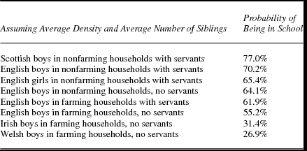
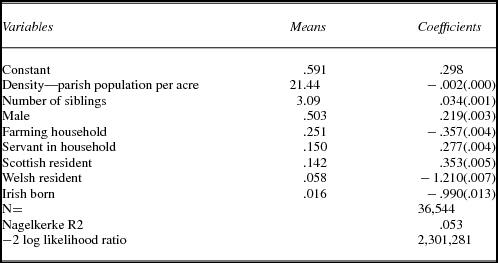
I took another look at the 1851 census data for children ages six through nine with a somewhat different specification, one that included girls and covered not just England but also Scotland and Wales and differentiated between those born in those countries versus the Irish born. It is a large data set, so all the variables achieved statistical significance, but few produced much change in the probabilities of being schooled in that year, as table 4 demonstrates. (See appendix 2 for the coefficients from the logit regression.) Held constant are two variables with very modest impact—number of siblings, which was positive, indicating that greater numbers of children in the family did not lead to dropouts, and density, which had a very small negative coefficient, suggesting residence in a town or the countryside made little difference. Table 3 shows that living in a farming household, the sector variable, brought down the probability by about nine points; having no servants, the economic class variable, lowered it by six points; and being a girl brought it down about five points. When I did further analysis, comparing children who lived with a farmer versus with an agricultural laborer, no statistical difference existed, implying that it was the agricultural sector not the class status that interfered with primary schooling.Footnote ¹³ The big news in table 4, though, relates to the Celtic fringe variables that, like the free black variable in US regressions on enrollment, greatly lower the probability of being in school.Footnote ¹⁴ Living in Scotland increased the likelihood of school enrollment, while living in Wales or being Irish born dramatically lowered it, holding other variables constant. English boys living in farm households with no servants had a 55.2 percent probability of being enrolled, while among the Irish born with the same profile it fell to less than a one in three chance and for Welsh lads just under 27 percent or half the chance of English boys. The sharp drop in the likelihood of enrollment due to being Welsh or being Irish born, even after controlling for other variables, point not only to poverty among these groups that did not get measured by the servant variable but also to cultural and language issues in getting children to go to school, issues that with a few exceptions (Mason Reference Mason1985) are understudied in the educational literature on Britain.

TABLE 4.

Probability of British children 6 to 9 years being enrolled, 1850–51

Source: See table 2.

Note: For coefficients that produced the probabilities, see appendix table A2.

As with Jason Long's regression discussed initially, the amount of variation explained in table 4 is quite meager, 5.3 percent, and mostly attributable to ethnicity. If economic factors had such a limited role in predicting enrollment for children of this age and geographical access did not appear to be a big problem—judging by the negative coefficient on the density variable—what was going on with the almost 40 percent of six to nine year olds of English and Scottish descent not registered in 1851 especially those in nonfarming households? With enrollment between ages six and nine ranging between 56 to 62 percent (see table 2), should we assume that the same children enrolled each year and the remaining 40 percent never darkened the door of a schoolhouse, or that regular attendance day in and day out and year in and year out was not the modal practice, even though compared to children in the United States instruction was focused on a smaller range of years? The weak performance of so many variables except the ethnic ones in the regression (see appendix 2) suggests the latter assumption makes the most sense. The choice of what year and how many days to go in that year may have a large random component because desultory attendance was the norm. So the next question, which goes beyond the materials studied here, is why does one see this pattern of casual enrollment when charity schools, workhouse schools, church-funded schools, privately endowed schools, cheap venture schools, plus parliamentary grants and local government support were all out there seeking to mold young minds whether said minds wanted to be molded or not (Mitch Reference Mitch1992: 111–26). The government in its reports stressed support for schooling that taught all children to “learn to read and write with tolerable ease, and to cipher well enough for the purposes of their condition in life, besides being grounded in the principles of religion.” Officials aimed at “regularity of the attendance, rather than to prolonging its duration,” meaning children under 10 were the target. Statements of this type suggest a hard road ahead for the working-class child who hoped to go on to secondary school (Humphries Reference Humphries2010: 316–19, 329) but also indicate a commitment to getting all children in the core age group educated in the 3Rs.Footnote ¹⁵ Was the quality of the education so poor or perceived as so irrelevant that parents saw no reason to waste their children's time with regularized enrollment every year when work or even play seemed more rewarding? If it was the sheer need for the wages of children under 10, why were the class indicators so weak? Long's own research (Reference Long2006), showing very small returns to education in the nineteenth century, may shed some light on this question. Whatever the answer, elitism and a restricted franchise do not appear the major forces in keeping most primary aged students from the classroom.

US School Funding in 1850 and the Role of Grassroots Democracy

That the first half of the nineteenth century witnessed a dramatic increase in the proportion of free white men who participated in elections and partisan activities is a commonplace of American political history. The impetus for common school reform has usually been envisioned as a reaction to rather than a result of this expansion in the franchise. That is, institutional and social histories concerning the rise of common school standards and financial support attribute the movement to state-level actions championed by Whig Party adherents, a major component of which was the “New England Element.” Whigs feared the effects on the republic of an idle youth and uneducated electorate. This concern was not entirely disinterested, as they ascribed some of their defeats at the ballot box to the ignorance of their opponents’ supporters. Also teacher organizations grew more vocal, desiring better working conditions and steady pay. In contrast, Democratic state legislators, while waxing enthusiastically about the virtues of education, generally opposed state laws mandating or even permitting districts to tax, calling them Prussian and despotic, and represented their own position as the will of the people (Cubberley Reference Cubberley1934; Groen Reference Groen2008; Kaestle Reference Kaestle1983; Maddox Reference Maddox1918; Soltow and Stevens Reference Soltow and Stevens1981). Being able to control the labor and education of one's children was presented as a basic parental right and particularly resonated with the Catholic population, which feared Protestant indoctrination in public schools. Suspicions that public funding would be channeled to grammar schools, academies, and colleges patronized by the affluent rather than the primary schools attended by the average child also allegedly fed some of this opposition (Opal Reference Opal2004; Sklar Reference Sklar1993).

Go and Lindert's recent article (Reference Go and Lindert2010) linking the US 1850 county-level census data on enrollments with county-level election returns substitutes a grassroots democracy/redistributive argument for what some call external benefits; and others, from a different perspective, label a social control explanation; and yet a third group would define as social capital building. The authors report a positive and statistically significant relationship between the enrollment rates and the proportion of total votes represented by the white adult male population for counties with voter participation in the 50 to 80 percent range. Why 50 to 80 percent? Utilizing an ends against the middle model in which county voters’ willingness to contribute more tax money for schools depended on who participated in the election, they hypothesized that neither counties with low participation (where the antitax well-propertied dominated the voting) or near universal participation (where even the cash-starved poor exercised the franchise) would show much financial support for instruction. It was when a growing segment of a county's middling sorts whose children needed schooling went to the polls that taxes got raised and wealth redistributed. In their opinion, however, this model, only worked in the North not in the South, because southern legislatures gave little budgetary autonomy to counties, and so voters could not opt for better education in their communities.

Go and Lindert deserve credit for melding two data sets to measure the influence of political participation on mid-nineteenth-century enrollments, something that those adopting a more literary or institutional approach to analysis of the issue never attempted nationwide. Questions arise, however, as to the applicability of the model and the appropriateness of the dependent variable chosen. The political, demographic, and economic data available in the data set also present opportunities to test competing theories on the reasons for increased investment in education.

Results from two recent studies of nineteenth-century school funding do not offer much support for the ends against the middle theory when applied to the constituencies behind increased taxes or to their motivation. Stoddard (Reference Stoddard2009), using state-level data for both North and South in 1850 and 1860, chose total government funds for her dependent variable and an inequality measure, the gap between a state's mean and median income, to ascertain whether increased amounts of funding emanated from redistributive, as argued by Go and Lindert, or external benefits motives. If the relationship were positive, it would mean that greater inequality prompted voters to pursue redistributive actions, knowing that the bulk of the tax burden would fall on the affluent. Her analysis, however, showed a negative relationship, meaning the smaller the gap the greater the revenues for education, suggesting an external benefits motivation behind the financing of public schools. Stoddard's findings are more in step with the institutional and social historians’ view of school support coming from those concerned about modernizing society and social control. In addition, higher voter participation in her state-level analysis did not prove a statistically significant predictor of funding in two specifications and in a third, where p improved to .20, the franchise coefficient had a negative relationship to revenue.

Vollrath (Reference Vollrath2013) studied the same issue, the relationship between school funding and inequality but using county-level census data from 1890 with local property taxes per capita as the dependent variable and farm size as the explanatory variable of interest. For the northern counties, a negative relationship, as in Stoddard, existed between inequality levels and the value of tax receipts, and funding varied based on the average size of farms. Counties with a greater share of farms in either the smallest size category (0–49 acres) or the larger (100–999 acres) had higher taxes compared to the middle category (50–99 acres)—a middle against the ends result, which represents the opposite of the Go and Lindert assumptions. A higher proportion of large farms was “definitively positive for education spending” (ibid.: 278), suggesting again external benefits as the major motivator. Of course, Vollrath deals with a later time period when tax-supported public schooling had achieved much more acceptance, and Stoddard relies on state-level data that cannot measure local grassroots sentiments.

What happens with the 1850 data when taxes rather than enrollments are used as the indicator of school support in counties? Per capita school taxes, not enrollment rates, seem to be the logical choice for a dependent variable, if the prime interest is in demonstrating grassroots support for schools. The county enrollment rate contains a sizeable measurement error, because, as noted earlier, the denominator does not accurately reflect the population at risk to be in the numerator. The total enrollment in school could be youth of any age, yet it is calculated as a percentage of free children ages 5 through 14. In this census, one out of every four counties in the North had more children enrolled in its schools than 5 to 14 year olds actually living in the county. The age distribution of students in 1850 discussed earlier in table 2 provides the best clue as to what is really being measured in the ratio of a county's enrollments to children ages 5 through 14. The table revealed the high proportion reported in school after age 14 and appendix 1 demonstrates that this educational sprawl disproportionately occurred in rural areas as opposed to urban centers. As a result, part of the high enrollment registered in counties is really the result of so many students over the age of 14 still enrolling for short periods to become literate and is associated with poorly funded one room schools. Interestingly, Goldin and Katz (Reference Goldin and Katz2008: 158) interpreted the decline between 1850 and 1880 in the proportion of students 14 and older still enrolled as a positive development, which in their view signaled more regularized schooling at younger ages and better educated students.

The argument that “the distribution of local political voice appears to be a robust predictor of tax support” (Go and Lindert Reference Go and Lindert2010: 1) actually has never been tested. The closest attempt was a regression showing a rise in the value of all government funds produced by an increase in the voting share among that group of northern counties where the share ranged from 50 percent to 80 percent—the middle group in a theory of the ends against the means model (Go and Lindert Reference Go and Lindert2007: 40). The problem is that total government funds include state and federal monies that have little to do with clamor within a community to raise taxes to support schools. The report on 1850 public school income (US Census 1854b: 141–42), which describes the data used in this analysis, separates government funds into those coming from (1) “taxation,” which meant taxes in townships, counties, and school districts; and (2) those emanating from “public funds” furnished largely by state land sales, miscellaneous state revenues, and federal deposit funds given to states (Swift Reference Swift1911). In 1850, the first constituted 49 percent of public school income and the second constituted 27 percent, the remainder coming from charging parents in rate bills to cover shortfalls or to extend the term for their own children. States varied a great deal, though, as to which category of school income was more important. In 6 of the 16 northern states and 9 out of 13 of the southern states, the public funds outstripped those collected from taxes. State-level officials, usually Whig, often set up these “public funds” to force recalcitrant localities to improve their schools (Kaestle Reference Kaestle1983; Maddox Reference Maddox1918). Thus the taxation source needs to be the one used to test grassroots enthusiasm.

The 1850 county-level data also allow for a testing of alternative explanations for the growth in the support of schools in the North. It would seem that the partisan complexion of a county—whether the Democrats or the Whigs held sway—more than the level of voting would determine the amount spent on taxes, given the importance attached to the differing viewpoints in the historical literature. In addition, behind political choice stand certain social and economic factors that have been at one time or another associated with promoting or retarding the expansion of schooling. Standard modernization theory holds that the Industrial Revolution and urbanization forced a human capital upgrade on a reluctant agrarian population, while an alternative rendering has industrialism as an impediment to continued education of youth due to labor demands. Thus the proportion urban, the proportion agricultural, and the fertility rate have been important factors incorporated into almost all national and state studies of nineteenth-century mass education (Field Reference Field1979). Increasingly, however, doubts have been raised about parts of the formulation. Most particularly the notion that in the mid-nineteenth century urban children received more education than agrarian youth has been challenged (Beadie Reference Beadie2010; Kaestle and Vinovskis Reference Kaestle and Vinovskis1980). As educational sprawl may account for the countryside outperforming cities, though, these variables merit another look.

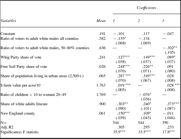
Table 5 displays the results for northern counties from three OLS regressions using the same aggregate census and election data sets for 1850 Go and Lindert employed (Haines Reference Haines2004; Clubb et al. Reference Clubb, Flanigan and Zingale1986) but substituting, as the dependent variable, the amount of school taxes levied per capita.Footnote ¹⁶ In the North, a majority of counties in 1850 reported levying school taxes. The independent variables reflect the competing theories as to what fueled the funding of a common school reform movement. Regressions 1 and 2 in the table feature the electoral participation variable. In the first the coefficient is strongly significant, but in the wrong direction. An increase in the percentage of white male voters reduces the per capita dollar value of the school tax. In the second regression, the coefficient is also negative but misses the .05 level of significance. As Go and Lindert stipulated an ends against the middle model, expecting just those counties with turnout percentages between 50 and 80 percent to have a positive effect on schooling, regression 3 tests that version of the variable, which eliminates more than 150 counties. The same result surfaces as in regression 1—the expansion of the electorate lessens tax support. Basically, the relationship is inverse.

TABLE 5.

Predictors of county school tax $ per capita, northern US counties in 1850 (OLS regression)

Source: Haines Reference Haines2004; Clubb et al. Reference Clubb, Flanigan and Zingale1986.

Note: Numbers in parentheses are standard errors, the asterisks indicate significance at the .05*, .01**, and .001*** levels. All coefficients had tolerance levels of .6 or higher. Percentage foreign born and amount per capita in manufacturing were not significant in any regressions and are not included. Counties in the regression come from New England, mid-Atlantic including Delaware, the east north central states, and Iowa. Two outliers were removed from $ value per acre of farms.

It is an open question as to how much of the variation in voter turnout can be attributed to wealth in the highly partisan period around 1850. By 1850 most adult white men who wanted to vote could vote, property qualifications having been abandoned as party rivalry heated up, and localities loosely enforced franchise requirements, if one were the right race and sex. Studies of antebellum electoral behavior attribute turnout to partisan competition and loyalty (Altschuler and Blumin Reference Altschuler and Blumin1997; Shade Reference Shade1987; Winkle Reference Winkle1983, Reference Winkle1992).

In terms of partisan influences, the coefficients in regressions 1 and 2 show that those counties with greater percentages of Whig or Free Soil voters did indeed have higher school taxes. In regression 3, with a smaller number of cases, the coefficient for Whig vote is still positive. The presence of the geographic variable New England assures us that even with the variation of the region most associated with public schooling and moral reform removed, the partisan results remain. The effect is broader than just New England.

Several variables in table 5 suggest that the countryside was seriously conflicted about increases in school funding. Regression 1 shows the positive effect of counties with an urban component and higher valued farm acreage. Regression 2 demonstrates the negative effect of high fertility rates on school taxes. High collinearity between farm values and fertility required they be put in separate regressions. While counties with high-fertility households that would be producing many potential students might have the most need for schooling, such counties did not opt to raise more taxes, even though wealthier households would feel the impact more than poorer ones. The negative correlations between high fertility and both urban dwellers and farm values hint at why. The youthfulness of high-fertility families and the burden of supporting those not yet of working age makes the fertility variable—the ratio of children less than 10 to women ages 20 through 49—a good proxy for newer settlements, low density, and lesser farm value. With unprecedented levels of internal migration in the first four decades of the nineteenth century, such families were common and usually found in counties where schools could not easily be accessed. These variables along with the Whig Party results suggest that wealthier counties supported school taxes if only from a desire to mold youth and modernize society. School funding fared best in higher density areas where fewer struggling farmers lived and attending classes posed less of a problem. The receptivity to extended amounts of schooling in low density areas (Parman Reference Parman2012) comes at a later point under different circumstances.

As these regressions are cross-sectional, how do we know that the causal arrows do not point in the opposite direction from what has been hypothesized? That is, perhaps higher school taxes in a community raised land values and stimulated urban migration as people searched for better quality schools. Both of these hypotheses, which make perfect sense in contemporary America, strain credulity a bit for 1850. But perhaps someone could make up a plausible argument for an endogenous relationship. One way to take care of such a problem is setting up difference equations, comparing change in variable from 1840 to1850 (Go and Lindert Reference Go and Lindert2010). The trouble with that strategy is that the social statistics for 1840 are notoriously inaccurate (Anderson Reference Anderson1988), a fact even recognized by those at the time. The US census office completely reorganized their procedures for the 1850 enumeration. There is an 1850 variable, however, percentage of white adults literate, which can stand as a crude measure of preexisting educational level and school quality. It is crude because it has a great deal of measurement error as far as absolute values are concerned: the statistic relies on the household head's word as to who could read and write. But the variable does reflect the relative differences in literacy among counties and states. In table 5 it serves the purpose of soaking up increases in school taxes that might be attributed to earlier increases pre-1850. As the entry of this variable made no difference, it does not seem that people migrated to high-tax areas for the schools but that counties with higher land values opted to fund schools at a higher level.

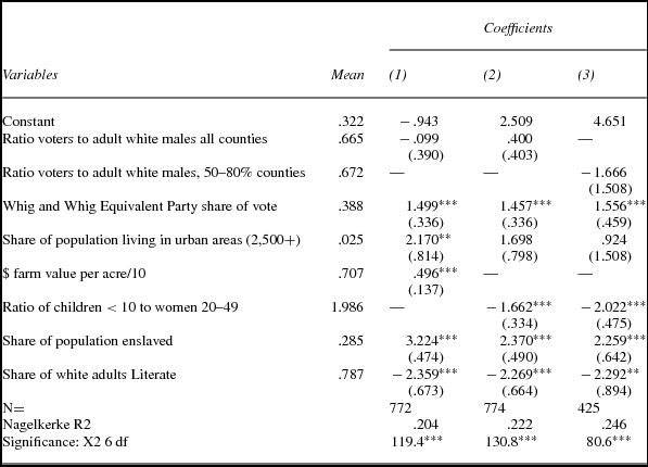
Interestingly, no one has argued that heightened white male electoral participation in the antebellum South led to more tax support for schools. Go and Lindert hypothesized that, unlike the North, southern communities lacked the local autonomy necessary to hike taxes for education. Yet some states—Maryland, Virginia, North Carolina, Mississippi, Louisiana, and Missouri—permitted communities to raise taxes for local schools and other states passed legislation for particular communities to have that right. The data set shows that 3 out of every 10 southern counties had some sort of school tax funding by 1850.Footnote ¹⁷ While that proportion allows analysis, it seemed best to use a binary logit regression to predict which counties did and did not have these levies rather than trying with OLS to explain the amount raised, as was done with the northern counties. An additional independent variable, not used in the northern state regression, was also inserted: the percentage of the population enslaved serves both an indicator of a southern county's wealth and its educational environment.

Table 6 finds a bit more similarity between the prewar North and South in the school tax regressions than might have been thought. The expansion of the electorate made no statistically significant difference, as Go and Lindert hypothesized for the region, but that does not mean politics played no role. As in the North, the higher the percentage of Whig or parties similar to Whig votersFootnote ¹⁸ the more likely the county had a school tax. As in the North, high-fertility counties, where the schooling needs were greatest, shunned school taxes. The power of this variable wiped out the positive zero order correlation between school taxes and urban areas. Contemporary southern commentators considered the sparse settlement of the white population to be the biggest barrier to mandating public school taxes (Kaestle Reference Kaestle1983: 203–4; Maddox Reference Maddox1918). The exclusion of the enslaved population from schooling exacerbated this low-density problem: 50 percent of southern counties had a quarter or more of their population unfree and legally prohibited from receiving instruction. Most of the differences between North and South also stem from the anomalous situation in which the wealthiest and best educated counties, as indicated by the white literacy variable, also had the most slaves. Literacy had a negative relationship with presence of a school tax yet was positively correlated with the amount of the school tax. Quite possibly private schooling already took care of white children's instructional needs in many affluent areas with high slave to free ratios. The behavior of the literacy variable, though, could be signaling that if one wants to search for some portion of the United States where redistributive motives in voting for school taxes might surface, certain areas in the South might be the place.

TABLE 6.

The probability of a southern county having a school tax in 1850 (binary logistic regression)

Source: See table 5.

Note: Numbers in parentheses are standard errors, the asterisks indicate significance at the .05*, .01**, and .001*** levels. Southern states are Maryland to Missouri southward to Texas. South Carolina was excluded due to a lack of electoral information.

Concluding Remarks

In this reexamination and reworking of recently available data on the degree of primary schooling and educational investment in the United States and Great Britain circa 1850, I found no clear-cut evidence that America soared ahead or that expanding the white male franchise in the United States boosted support for schools. The perceived US advantage in regard to schooling is due to an underestimation of the population at risk, a conflation of enrollments with attendance, and ignoring differences in the length of school terms. Politics did have an effect on US school investment: counties that elected Whig and antislavery party candidates to Congress also paid more per capita in school taxes and those voting Democratic paid less. The Whigs, though, were associated with external benefits and social control arguments about the need for better schools, not populist redistributive motives, and their political opponents often accused them of undemocratic tendencies. Considerable support for schools came from the state and even federal levels. The Civil War put the school reformers into the drivers’ seat for the rest of the nineteenth century, and compulsory primary education continued to be high on their agenda. Just as the expanded white male franchise does not explain better funded schools, social class in Britain appears to have played very little role in restricting school enrollment at the primary level. Heavy discrimination entered in after that point. As in the United States, British officialdom by 1850 embraced regularized schooling for elementary age students, but it is not clear all parents and children saw the advantages. Demographic variables, other than those measuring ethnic differences, offer little in the way of explaining why particular British students under 10 years failed to enroll in a particular year.

Rather than supporting an American exceptionalism explanation, the results encourage the adoption of a North Atlantic perspective on the mid-nineteenth-century spread of primary schooling and the acquisition of the 3Rs. Mid-century modernizers, citing popular ignorance and the need for moral reform, dominated the push for more extensive and thus more costly schooling in both nations, and in both nations they were viewed by significant numbers of parents and voters as wrongheaded. In the United States, educational sprawl prevailed in the kind of low-density agricultural areas described by Fischel (Reference Fischel2009). In more industrialized Great Britain, a short concentrated dose of instruction remained the norm for youth soon to be recruited into the workforce. Learning by doing rather than by classroom lessons retained popularity. The most extreme barriers/hostility to increased schooling involved racial, ethnic, and language differences among those providing the services and those supposed to be their customers. The focus needs to move from enrollments—almost all free children by the mid-nineteenth century enrolled in school for multiple, though not necessarily consecutive, years—and deal more directly with the reasons certain groups of enrollees ducked in and out of class so routinely and why they eventually stopped.