1. Introduction
It is commonly accepted that magnetohydrodynamic (MHD) induction processes are responsible for the development of self-sustained magnetic fields in astrophysical bodies (Roberts & Glatzmaier Reference Roberts and Glatzmaier2000); a process known as the dynamo instability, converting kinetic energy into magnetic energy. In the context of a planetary dynamo, occurring in liquid metals, the base flow is always highly turbulent. Experimental evidence of the dynamo instability has been obtained from model flows in the early years of this millenium (Gailitis et al.
Reference Gailitis, Lielausis, Dement’ev, Platacis, Cifersons, Gerbeth, Gundrum, Stefani, Christen, Hanel and Will2000; Stieglitz & Müller Reference Stieglitz and Müller2001). Since then many attempts have been made to generate less constrained dynamos (Peffley, Cawthorne & Lathrop Reference Peffley, Cawthorne and Lathrop2000; Nornberg et al.
Reference Nornberg, Spence, Kendrick, Jacobson and Forest2006; Frick et al.
Reference Frick, Noskov, Denisov and Stepanov2010; Colgate et al.
Reference Colgate, Beckley, Si, Martinic, Westpfahl, Slutz, Westrom, Klein, Schendel, Scharle, McKinney, Ginanni, Bentley, Mickey, Ferrel, Li, Pariev and Finn2011). Due to the turbulent nature of the flows, reaching the magnetic Reynolds number critical value (
 $\mathit{Rm}_{c}$
, for which induction processes balance ohmic dissipation) requires considerable injected mechanical power. As a result, experiments are often designed or engineered so that
 $\mathit{Rm}_{c}$
, the threshold value, is optimized to lie within the operational limits,
 $\mathit{Rm}_{c}<\mathit{Rm}^{max}$
, where
 $\mathit{Rm}^{max}$
is the maximum value achievable in the considered set-up.
In the von Kármán sodium experiment (VKS), dynamo action has been achieved by generating the flow motions using impellers made of soft iron (Monchaux et al.
Reference Monchaux, Berhanu, Bourgoin, Moulin, Odier, Pinton, Volk, Fauve, Mordant, Pétrélis, Chiffaudel, Daviaud, Dubrulle, Gasquet, Marie and Ravelet2007, Reference Monchaux, Berhanu, Aumaître, Chiffaudel, Daviaud, Dubrulle, Ravelet, Fauve, Mordant, Pétrélis, Bourgoin, Odier, Pinton, Plihon and Volk2009). From a similar base flow, we consider here another example, in which the dynamo cycle is partially synthetic. The principle, inspired by the Bullard dynamo scheme (Bullard Reference Bullard1955), relies on an external amplification of electrical currents in coils, driven by a turbulent induction process. The fluid induction process is a turbulent omega effect coupled with a boundary condition effect (referred to as the BC-effect as in Bourgoin et al.
Reference Bourgoin, Volk, Frick, Khripchenko, Odier and Pinton2004 and Verhille et al.
Reference Verhille, Plihon, Bourgoin, Odier and Pinton2010), while the external amplification mimics an alpha effect (a mechanism which generates an induced current parallel to the magnetic field). The second mechanism, being linked to an electronic amplification of gain
 $A$
, will be referred to as ‘A’ for amplification. The dynamo mechanism is then labelled the A–BC dynamo. This experimental set-up is able to generate dynamo action at
 $\mathit{Rm}_{c}\sim 1$
, far below the natural critical value of the base flow (
 $\mathit{Rm}_{c}\sim 50$
estimated in kinematic simulations (Ravelet et al.
Reference Ravelet, Chiffaudel, Daviaud and Léorat2005), and
 $\mathit{Rm}_{c}\sim 40$
in the VKS experiment). This Bullard–von Kármán dynamo was originally studied by Bourgoin et al. (Reference Bourgoin, Volk, Plihon, Augier, Odier and Pinton2006) who documented the development of the instability, then by Verhille et al. (Reference Verhille, Plihon, Fanjat, Volk, Bourgoin and Pinton2010) who detailed the importance of large-scale flow dynamics on the development of dynamical regimes. In these previous works, the saturation was due to current limitations in the external coils, and the magnitude of the dynamo field remained too weak to significantly modify the flow, confining these studies to kinematic regimes. In the work detailed in the present article, the available electrical currents have been increased, and the self-sustained magnetic field now reaches values such that Lorentz forces modify the bulk of the von Kármán flow.
While the effect of Lorentz forces on the momentum balance of turbulent flows has been studied in various experiments involving applied magnetic fields (Alemany et al. Reference Alemany, Moreau, Sulem and Frisch1979; Sommeria & Moreau Reference Sommeria and Moreau1982; Brito et al. Reference Brito, Cardin, Nataf and Marolleau1995; Sisan, Shew & Lathrop Reference Sisan, Shew and Lathrop2002; Klein & Pothérat Reference Klein and Pothérat2010; Verhille et al. Reference Verhille, Khalilov, Plihon, Frick and Pinton2012; Cabanes, Schaeffer & Nataf Reference Cabanes, Schaeffer and Nataf2014), very little is known in dynamo configurations. In the Riga experiment a slowing down of the axial flow as well as a modification of the swirling profile have been observed (Gailitis et al. Reference Gailitis, Lielausis, Platacis, Gerbeth and Stefani2003). Similarly, in the Karlsruhe experiment, a slow down of the axial motion has been recorded at saturation (Müller, Stieglitz & Horanyi Reference Müller, Stieglitz and Horanyi2004), which also led to an estimation of the dynamo energy budget. In the VKS experiment, the modification of the flow at saturation has been too weak to allow significant measurements. The main asset of the Bullard–von Kármán set-up considered here is that sufficiently large magnetic fields can be reached in a dynamo configuration, modifying the bulk flow. We show here that the von Kármán flow is modified in the bulk by Lorentz forces in the dynamo regime. In addition to the supercritical bifurcation of the magnetic field, the Bullard–von Kármán dynamo displays a bifurcation of liquid gallium flow, from a hydrodynamic base flow (for which the effects of the magnetic field on the flow are negligible) below dynamo onset to an MHD saturated flow (for which the back reaction of the magnetic field on the flow is significant) above onset.
The article is organized as follows. Details of the experimental set-up and dimensionless parameters are given in § 2. The supercritical dynamo bifurcation is then investigated in detail in § 3: the magnetic field bifurcates via an on–off intermittent scenario, and then modifies the bulk flow. The bifurcation towards an MHD saturated state and the associated power budget is then analysed. We discuss dynamical regimes, namely polarity inversions, in § 4. As an illustration of the versatility of the system, a self-killing dynamo regime as well as a subcritical dynamo set-up for which the dynamo action is only observed from an MHD base flow, are demonstrated in § 5. Finally, further implications of the dynamo power budget are discussed in § 6.
2. Experimental set-up and dimensionless parameters
The experimental system involves the motion of liquid gallium and the dynamics is governed by the coupled set of the incompressible Navier–Stokes (NS) and induction equations:
 $$\begin{eqnarray}\displaystyle & \displaystyle \partial _{t}\boldsymbol{u}+(\boldsymbol{u}\boldsymbol{\cdot }\boldsymbol{{\rm\nabla}})\boldsymbol{u}=-\frac{\boldsymbol{{\rm\nabla}}p}{{\it\rho}}+{\it\nu}{\rm\nabla}^{2}\boldsymbol{u}+\frac{\boldsymbol{j}\times \boldsymbol{B}}{{\it\rho}}, & \displaystyle\end{eqnarray}$$
 $$\begin{eqnarray}\displaystyle & \partial _{t}\boldsymbol{B}+(\boldsymbol{u}\boldsymbol{\cdot }\boldsymbol{{\rm\nabla}})\boldsymbol{B}=(\boldsymbol{B}\boldsymbol{\cdot }\boldsymbol{{\rm\nabla}})\boldsymbol{u}+{\it\lambda}{\rm\nabla}^{2}\boldsymbol{B}, & \displaystyle\end{eqnarray}$$
 $$\begin{eqnarray}\displaystyle & \boldsymbol{{\rm\nabla}}\boldsymbol{\cdot }\boldsymbol{u}=0 & \displaystyle\end{eqnarray}$$
 $$\begin{eqnarray}\displaystyle & \boldsymbol{{\rm\nabla}}\boldsymbol{\cdot }\boldsymbol{B}=0 & \displaystyle\end{eqnarray}$$
 $\boldsymbol{u}(\boldsymbol{r},t),p(\boldsymbol{r},t),\boldsymbol{B}(\boldsymbol{r},t)$
and
 $\boldsymbol{j}(\boldsymbol{r},t)$
are velocity field, pressure, magnetic field and current density respectively. The fluid density of liquid gallium is
 ${\it\rho}=6100~\text{kg}~\text{m}^{-3}$
, the kinematic viscosity
 ${\it\nu}=3.1\times 10^{-7}~\text{m}^{2}~\text{s}^{-1}$
and the magnetic diffusivity
 ${\it\lambda}=1/({\it\mu}_{0}{\it\sigma})=0.2~\text{m}^{2}~\text{s}^{-1}$
(with
 ${\it\mu}_{0}$
the magnetic permeability of vacuum and
 ${\it\sigma}=3.9\times 10^{6}~\text{S}~\text{m}$
, the electrical conductivity of liquid gallium). The nature of the problem is governed by the values of the main dimensionless parameters expressed using the integral scale of the experiment,
 $L$
, and the characteristic velocity
 $U$
(computed as the tip velocity of the impellers, see the next subsection): the kinetic Reynolds number
 $\mathit{Re}=UL/{\it\nu}$
(which compares the amplitude of the inertial term to the viscous term in the Navier–Stokes equation (2.1)), the magnetic Reynolds number
 $\mathit{Rm}=UL/{\it\lambda}={\it\mu}_{0}{\it\sigma}LU$
(which compares the induction term to the diffusion term in the induction equation (2.2)) and the interaction parameter
 $N=|\boldsymbol{j}\times \boldsymbol{B}|/|{\it\rho}(\boldsymbol{u}\boldsymbol{\cdot }\boldsymbol{{\rm\nabla}})\boldsymbol{u}|$
which compares the amplitude of the Lorentz force to the inertial term in the Navier–Stokes equation, see § 2.3 for details.
2.1. A von Kármán gallium flow
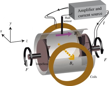
The experimental set-up is sketched in figure 1 and described in detail in Verhille et al. (Reference Verhille, Plihon, Fanjat, Volk, Bourgoin and Pinton2010). The liquid gallium flow is created by two coaxial counter-rotating impellers (stainless steel disks with radius
 $R_{d}=82.5~\text{mm}$
fitted with eight straight blades of height 10 mm). The stainless-steel cylinder enclosing the flow has a radius
 $R_{0}=97~\text{mm}$
(which will be used as a characteristic length scale of the dimensionless numbers of the problem
 $L\sim R_{0}$
). The impellers are driven by two 10 kW AC-motors with rotation rate
 $F$
adjustable up to
 $F^{max}=20~\text{Hz}$
. For each run, the motors are operated at constant rotation speed and the motors’ electric drives deliver an analogue output proportional to the current in the motor, as a measurement of the applied mechanical torque
 ${\it\Gamma}$
.
Sketch of the experimental Bullard–von Kármán set-up. The flow, created by the rotation of impellers at frequency
 $F$
, induces a component
 $B_{z}$
(in the axial direction) in the presence of a field
 $B_{x}$
(in the transverse direction). The value of the induced field
 $B_{z}$
measured by a Hall sensor is amplified and drives the power supply which delivers the current in the transverse coils.

The integral kinetic Reynolds number computed using the velocity of the impeller and the radius of the vessel
 $R_{0}$
is
 $\mathit{Re}\sim 10^{6}$
; therefore the flow is fully turbulent. The time-averaged flow consists of two counter-rotating toroidal cells with recirculating poloidal cells created by the centrifugal ejection of the fluid by the rotation of the impellers. In an exact counter-rotating regime, these cells form a shear layer in the mid-plane, and detailed experimental investigations of time-averaged flow topologies, fluctuation levels and characteristics may be found in Ravelet, Chiffaudel & Daviaud (Reference Ravelet, Chiffaudel and Daviaud2008).
The magnetic Reynolds number
 $\mathit{Rm}$
is typically of order 1, well below the critical value of 44 obtained for a similar flow in the VKS experiment (Monchaux et al.
Reference Monchaux, Berhanu, Aumaître, Chiffaudel, Daviaud, Dubrulle, Ravelet, Fauve, Mordant, Pétrélis, Bourgoin, Odier, Pinton, Plihon and Volk2009). A set of induction coils (of total resistance
 $R=0.28~{\rm\Omega}$
) creates a magnetic field transverse to the axis of rotation of the von Kármán flow, homogeneous to within 13 % over the flow volume, as shown in figure 1. The current
 $I$
in the coils is driven by a 10 kW bipolar power supply, with analogue control. The resulting transverse magnetic field
 $B_{x}={\it\kappa}I$
(where
 ${\it\kappa}$
is a constant depending on the characteristics of the coils) has a maximal intensity equal to 1200 G (0.12 T) in the flow vessel. The interaction of a transverse magnetic field
 $B_{x}$
with the turbulent motions of the flow induces an axial magnetic component
 $B_{z}$
through a mechanism, described in Bourgoin et al. (Reference Bourgoin, Volk, Frick, Khripchenko, Odier and Pinton2004) and Verhille et al. (Reference Verhille, Plihon, Bourgoin, Odier and Pinton2010), involving the shear layer dynamics in the mid-plane (omega-effect) and insulating boundary conditions forcing the current to loop back in the liquid gallium volume. This induction effect will be referred to as the BC-effect. In the limit of vanishingly small interaction parameter
 $N$
and moderate
 $\mathit{Rm}$
, the time-averaged axial magnetic field
 $\langle B_{z}\rangle$
scales linearly with
 $\mathit{Rm}$
,
 $$\begin{eqnarray}\langle B_{z}\rangle =k\,\mathit{Rm}\langle B_{x}\rangle \quad (N\rightarrow 0,~B<100~\text{G}),\end{eqnarray}$$
 $k$
being a geometric constant of order
 $10^{-2}$
and
 $\langle \cdot \rangle$
standing for time averaging.
When the interaction parameter
 $N$
is large, a nonlinear correction of functional form
 $$\begin{eqnarray}\langle B_{z}\rangle =k\,\mathit{Rm}(1-{\it\alpha}\sqrt{N})\langle B_{x}\rangle \quad (B>100~\text{G})\end{eqnarray}$$
has to be taken into account,
 ${\it\alpha}$
also being a geometric constant (Verhille et al.
Reference Verhille, Khalilov, Plihon, Frick and Pinton2012).
Magnetic fields are measured in the mid-plane using a Bell 9150 gaussmeter and Hall-effect probes (sketched as a vertical black tube in the figure 1). The probe measuring the
 $z$
component is located at a radius
 $r=0.9R_{0}$
close to the wall except in § 5 where it is located deeper. The
 $B_{x}$
component is measured on the coils’ axis at
 $r=0.55R_{0}$
(not shown). Data are recorded using a National Instrument digitiser NI 4472 at sampling frequency of 1 kHz and 24 bits resolution.
2.2. Semi-synthetic Bullard–von Kármán dynamo
The Bullard–von Kármán (BvK) set-up relies on an external feedback inspired by Bullard’s disk dynamo (Bullard Reference Bullard1955).
The dynamo mechanism may be split into two induction processes. The first one is the turbulent induction process described above, inducing an axial component
 $B_{z}$
from a transverse
 $B_{x}$
component through a turbulent BC-effect. The second one stems from the external amplification of the Hall-probe signal sampling the
 $B_{z}$
component of the magnetic field, which is used to control the power supply feeding the current into the transverse coils. This external feedback produces a transverse component
 $B_{x}$
of the magnetic field proportional to the turbulent-induced component
 $B_{z}$
:
 $$\begin{eqnarray}B_{x}=AB_{z},\end{eqnarray}$$
 $A$
being proportional to the gain of the amplifier. Thus, the complete mechanism of the present dynamo is referred to as an
 $A{-}BC$
type dynamo. The onset of the dynamo instability may be understood in the following way: combining the induction equation (2.5) with the external feedback (2.7) the magnetic energy grows from a vanishingly small magnetic field perturbation if
 $\mathit{Rm}>\mathit{Rm}_{c}=(kA)^{-1}$
. Since the amplification coefficient
 $A$
can be tuned, the threshold of the instability can be set arbitrarily (typically
 $\mathit{Rm}_{c}=(kA)^{-1}\sim 1$
) to values much lower than the expected one for homogeneous dynamos. In the remainder of this article, several values of the amplification
 $A$
will be presented; however, for the sake of simplicity, only the associated critical
 $\mathit{Rm}$
value,
 $\mathit{Rm}_{c}=(kA)^{-1}$
, will be specified. A first set of experiments using this arrangement has been reported in Verhille et al. (Reference Verhille, Plihon, Fanjat, Volk, Bourgoin and Pinton2010). Then, one was restricted to kinematic regimes because the maximum current delivered by the power supply limited the magnetic field amplitude to 60 G, and the interaction parameter
 $N$
to typically
 $10^{-4}$
; Lorentz forces were not strong enough to significantly modify the flow. The magnetic field at saturation was then set by the maximum current drawn from the power supply. However, several features were observed, such as dynamo states connected to ‘on–off’ intermittency, and field reversals. In the present set-up, not only is self-generation reached at
 $\mathit{Rm}\sim 1$
, but it is achieved in a fully MHD regime, so far restricted to large sodium flows (at low magnetic Prandtl number
 $\mathit{Pm}={\it\nu}/{\it\lambda}\sim 10^{-6}$
in liquid metals) or to computer simulations (at moderate to high
 $\mathit{Pm}$
).
The dynamo magnetic mode chosen in the present configuration (a transverse dipole relative to the axis of rotation of the impellers) should also be discussed further. Kinematic simulations (i.e. solving the induction equation as an eigenvalue problem from a prescribed velocity field) predict that the most unstable magnetic eigenmode is a transverse dipole when using the time-averaged von Kármán flow (Ravelet et al.
Reference Ravelet, Chiffaudel, Daviaud and Léorat2005). These simulations predict an onset of dynamo for
 $\mathit{Rm}$
of order 50. The configuration of the Bullard–von Kármán dynamo investigated in this article allows regimes to be studied where saturation is provided by Lorentz forces, at
 $\mathit{Rm}$
of order 1 (thanks to the external amplification) in the presence of a transverse dipole. The present study gives information about the full nonlinear coupled problem in the presence of a dynamo mode similar to the one predicted by kinematic simulations, at leading order. This is in sharp contrast with the experimental dynamo magnetic field observed in the VKS experiment (with soft iron impellers), which is an axial dipole (Boisson et al.
Reference Boisson, Aumaître, Bonnefoy, Bourgoin, Daviaud, Dubrulle, Odier, Pinton, Plihon and Verhille2012). The exact mechanism is still under investigation, but recent numerical simulations have highlighted that a small-
 ${\it\alpha}$
effect between the blades of the impellers, together with a high magnetic permeability of the impeller, could explain the observed magnetic dynamo mode (Giesecke et al.
Reference Giesecke, Nore, Stefani, Gerbeth, Léorat, Herreman, Luddens and Guermond2012; Nore et al.
Reference Nore, Léorat, Guermond and Giesecke2015).
2.3. Interaction parameter
The focus of the current study is on the dynamo characteristics in regimes where the bifurcated flow differs significantly from the original base flow. This occurs when Lorentz forces are sufficient to compete with other terms in the Navier–Stokes momentum equation (2.1). Some care is needed when expressing the interaction parameter
 $N$
as a function of the observables of the system. Depending on the system and on the values of the control parameters, several estimates of the Lorentz force can be derived in a system with characteristic length
 $L$
and characteristic velocity
 $U$
. We will assume that the velocity and magnetic field characteristic length scales have the same order of magnitude since in our gallium flow the magnetic field diffusion length (
 $L_{d}=\sqrt{{\it\lambda}/2{\rm\pi}F}\sim 5.9~\text{cm}$
for
 $F=10~\text{Hz}$
) is of the order of the shear layer thickness (note that since
 $L_{d}$
is comparable to the integral scale and to the characteristic length of the system
 $R_{0}$
, we choose to estimate the space variations of
 $\boldsymbol{B}$
using
 $L=R_{0}$
).
-
(a) In dynamo regimes (high
 $\mathit{Rm}$
values and absence of external magnetic fields), the current density is expressed as
$\boldsymbol{j}=\boldsymbol{{\rm\nabla}}\times \boldsymbol{B}/{\it\mu}_{0}$
. The interaction parameter is then estimated as (2.8)where
$$\begin{eqnarray}N^{dyn}=\frac{|(\boldsymbol{{\rm\nabla}}\times \boldsymbol{B})\times \boldsymbol{B}|}{|{\it\mu}_{0}{\it\rho}(\boldsymbol{u}\boldsymbol{\cdot }\boldsymbol{{\rm\nabla}})\boldsymbol{u}|}\sim \frac{B^{2}}{{\it\rho}{\it\mu}_{0}U^{2}}\end{eqnarray}$$
$B$
is the amplitude of the total magnetic field created by the flow motions. This is the typical expression used in astrophysics, for which
$\boldsymbol{B}$
depends on
$\boldsymbol{u}$
through dynamo scaling laws.
-
(b) In induction regimes (moderate
$\mathit{Rm}$
values and presence of an external magnetic field
$\boldsymbol{B}^{E}$
), a magnetic field
$\boldsymbol{b}^{I}$
is induced by the interaction of the flow with the external and homogeneous magnetic field
$\boldsymbol{B}^{E}$
. The current density in the fluid is expressed as
$\boldsymbol{j}=\boldsymbol{{\rm\nabla}}\times \boldsymbol{b}^{I}/{\it\mu}_{0}$
, and the interaction parameter is estimated as (2.9)In the linear regime
$$\begin{eqnarray}N^{ind}\sim \frac{b^{I}(B^{E}+b^{I})}{{\it\mu}_{0}{\it\rho}U^{2}}.\end{eqnarray}$$
$b^{I}\sim \mathit{Rm}\,B^{E}$
and usually
$b^{I}\ll B^{E}$
in liquid metal flows at
$\mathit{Rm}\sim 1$
. This leads to (2.10)where
$$\begin{eqnarray}N^{ind~linear}\sim \frac{B^{2}{\it\sigma}L}{{\it\rho}U}\end{eqnarray}$$
$B$
is the amplitude of the external magnetic field (or equivalently the amplitude of the applied magnetic field). This is the typical expression used in induction experiments, for which
$\boldsymbol{B}$
and
$\boldsymbol{u}$
are independent.
-
(c) In the context of the Bullard–von Kármán dynamo considered here, the induced magnetic field (
$b^{I}=B_{z}$
) actually drives the external magnetic field (
$B^{E}=B_{x}$
), through the amplification feedback
$B_{x}=AB_{z}$
, so that the interaction parameter can be estimated as (2.11)where
$$\begin{eqnarray}N^{BvK}=A\frac{B_{z}^{2}}{{\it\mu}_{0}{\it\rho}U^{2}}\end{eqnarray}$$
$B_{z}$
is the magnetic field created (induced) by the flow motions. One recovers the dynamo expression, in which the amplification factor
$A$
shows clearly that the external amplification is used to produce a large impact of the magnetic field on the flow. There is an equivalent expression, valid when the magnetic induction remains linear in
$\mathit{Rm}$
(
$\langle B_{z}\rangle \sim \mathit{Rm}\langle B_{x}\rangle$
, i.e. for moderate values of the interaction parameter
$N$
), and thus valid close to dynamo onset
$N^{BvK\,onset}\sim (B_{x}^{2}{\it\sigma}L/{\it\rho}U)$
. One recovers the induction expression, but in a dynamo configuration, for which
$\boldsymbol{B}$
is not independent of
$\boldsymbol{u}$
.


These equivalent formulations of
 $N$
result from the nature of the Bullard–von Kármán set-up: a dynamo set-up from a semi-synthetic feedback relying on a turbulent induction process from an externally applied magnetic field.
3. Supercritical bifurcation and saturation
3.1. Bifurcation
In this section, we focus on the onset of the instability and on the description of dynamo regimes. The control parameter of the dynamo bifurcation is the magnetic Reynolds number
 $\mathit{Rm}=2{\rm\pi}{\it\mu}_{0}{\it\sigma}R_{0}^{2}F$
, and is varied by modification of the rotation rate of the impellers
 $F$
from 0 to
 $F^{max}$
. In the remainder of this article, we will study the behaviour of the dynamo magnetic field through the evolution of moments of the
 $B_{x}$
component of the magnetic field, which for the sake of simplicity will be denoted
 $B$
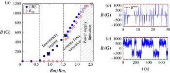
. Figure 2(a) shows a typical bifurcation diagram, i.e. the evolution of the magnetic field while increasing the magnetic Reynolds number
 $\mathit{Rm}$
. Following the kinematic approach presented in § 2.2, the critical value of self-excitation is expected to be
 $\mathit{Rm}_{c}=(kA)^{-1}=1.94$
for the chosen amplification. For reasons that will soon be clear, the behaviour of the dynamo field is tracked using two indicators: the time-averaged value and the most probable value of the norm of the dynamo magnetic field, respectively labelled
 $\langle |B|\rangle$
and
 $B_{mp}$
.
(a) Bifurcation diagram of the Bullard–von Kármán dynamo as a function of
 $\mathit{Rm}/\mathit{Rm}_{c}$
. Circles stand for the time average of the dynamo magnetic field
 $|B|$
and diamonds for the most probable value of
 $|B|$
. Squares mark the values for which time series are plotted in (b) and (c). The threshold for this run is
 $\mathit{Rm}_{c}=1.94$
. (b) Time series for
 $\mathit{Rm}/\mathit{Rm}_{c}=0.9$
, in the intermittent regime. (c) Time series for
 $\mathit{Rm}/\mathit{Rm}_{c}=1.6$
, in the Lorentz force saturation regime. Dashed lines mark the maximum value of the magnetic field
 $B^{max}$
which could be drawn if the current reached the maximum value allowed by the external power supply.

Below
 $\mathit{Rm}/\mathit{Rm}_{c}\sim 0.61$
, the magnetic field is vanishingly small. Slightly above, the dynamics of the magnetic field displays irregular bursts of activity, as shown in figure 2(b) at
 $\mathit{Rm}/\mathit{Rm}_{c}=0.9$
. Briefs periods of non-zero magnetic field are recorded, with both polarities being accessible due to the presence of additive noise in the loop, as noted in Verhille et al. (Reference Verhille, Plihon, Fanjat, Volk, Bourgoin and Pinton2010). In this regime the time-average value of the magnetic field grows steadily with
 $\mathit{Rm}/\mathit{Rm}_{c}$
(circles in figure 2
a), but its most probable value remains equal to zero (diamonds in figure 2
a). This regime extends for a range of
 $\mathit{Rm}/\mathit{Rm}_{c}$
values between 0.61 and 1.5 and is referred to as the ‘Intermittent regime’ in figure 2(a).
A transition is observed above
 $\mathit{Rm}/\mathit{Rm}_{c}=1.6$
: the most probable value of the magnetic field is no longer zero. It must be noted that this transition is associated with a steeper increase of
 $\langle |B|\rangle$
with
 $\mathit{Rm}/\mathit{Rm}_{c}$
, though without any discontinuity at
 $\mathit{Rm}/\mathit{Rm}_{c}=1.6$
. A typical time series of the magnetic field is shown in figure 2(c) over
 $700~\text{s}$
at
 $\mathit{Rm}/\mathit{Rm}_{c}=1.6$
. In either polarity state, the magnetic field saturates to a value which is less than the maximum value of the magnetic field
 $B^{max}$
(corresponding to the maximum current,
 $I^{max}$
, fed by the power supply, i.e.
 $B^{max}(I^{max})=1200~\text{G}$
). In this regime, and in contrast with the previous studies, the saturation of the dynamo magnetic field occurs from the action of the Lorentz forces and not from the material limitation imposed by the power supply driving the coils. Note also that the fluctuations in the magnetic field are of the same amplitude as its time-averaged value, a feature often observed in turbulent dynamos (Monchaux et al.
Reference Monchaux, Berhanu, Aumaître, Chiffaudel, Daviaud, Dubrulle, Ravelet, Fauve, Mordant, Pétrélis, Bourgoin, Odier, Pinton, Plihon and Volk2009). This regime, for which the dynamo magnetic field is saturated via the action of Lorentz forces acting in the bulk of the flow, extends for
 $1.6<\mathit{Rm}/\mathit{Rm}_{c}<2.16$
. It is denoted as ‘Lorentz force saturation’ in figure 2(a).
As
 $\mathit{Rm}/\mathit{Rm}_{c}$
is increased above 2.16, instantaneous values of the dynamo magnetic field reach the amplitude of the material limitation
 $B^{max}$
. At this point the dynamo field is saturated by material limitations rather than by the action of the Lorentz forces: the most probable value shows a concave evolution instead of the linear evolution in the Lorentz force saturation regime and saturates at
 $B^{max}$
(since excursions of the magnetic field are limited to
 $\pm B^{max}$
). This regime is denoted ‘Power supply limitation’ and its range is shown hatched in figure 2(a).
Since the most probable value
 $B_{mp}$
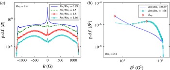
acts as an indicator of a transition between the intermittent and Lorentz force saturation regimes, further information is obtained from the probability distribution functions (p.d.f.) of
 $B$
as displayed in figure 3(a) (curves have been shifted for clarity) and
 $B^{2}$
in figure 3(b). In the intermittent regime (
 $\mathit{Rm}/\mathit{Rm}_{c}=0.89$
, solid curve and
 $\mathit{Rm}/\mathit{Rm}_{c}=1.5$
, dashed curve) the p.d.f. is maximum at
 $B=0$
, and displays extended lateral wings. In the saturated regime (
 $\mathit{Rm}/\mathit{Rm}_{c}=1.6$
, circles and
 $\mathit{Rm}/\mathit{Rm}_{c}=1.66$
, squares) the p.d.f. is bimodal with lobes centred at
 $B=\pm B_{mp}$
. The probability of having
 $B=0$
is still significant; this might be due to the fact that the magnetic field stays around zero for several turnover times during polarity inversions (see § 4). The transition between the intermittent and the saturated regime is statistically continuous as seen in the evolution of the p.d.f. between
 $\mathit{Rm}/\mathit{Rm}_{c}=1.5$
and 1.66. The value of the p.d.f. at
 $B=0$
slowly decreases, while the bimodal lateral wing bumps slowly increase.
 $B_{mp}$
bifurcates from zero to non-zero values at
 $\mathit{Rm}/\mathit{Rm}_{c}=1.6$
. In all cases, the p.d.f. displays local peaks at the highest amplitudes of
 $B\sim B^{max}$
, as a result of the power supply limitations.
(a) Probability distribution function of the dynamo magnetic field
 $B$
for various
 $\mathit{Rm}/\mathit{Rm}_{c}$
values (shifted for clarity). (b) Probability density function of the magnetic energy
 $B^{2}$
.

The following subsections discuss in detail the different regimes introduced here.
3.2. Intermittent regime
Previous studies on the kinematic regime of a BvK dynamo have characterized the observed intermittent regime close to dynamo onset as ‘on–off’ intermittency (Bourgoin et al.
Reference Bourgoin, Volk, Plihon, Augier, Odier and Pinton2006; Verhille et al.
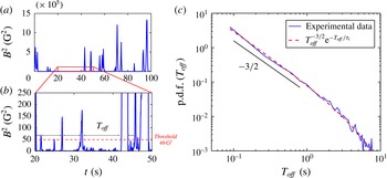
Reference Verhille, Plihon, Fanjat, Volk, Bourgoin and Pinton2010). On–off intermittency close to an instability onset is expected for fluctuating dynamical systems presenting an unstable invariant manifold in the phase space (Ott & Sommerer Reference Ott and Sommerer1994). The presence of a multiplicative noise (turbulent fluctuations) in a dynamical system creates fluctuations in such a way that the instantaneous growth rate of the magnetic field can be non-zero. Since, in our system, there is always an additive noise contribution (from the electronic noise and from turbulent induction arising from the ambient field), the intermittent signal close to dynamo onset displays both polarities. This intermittent regime is characterized by the statistics of the magnetic energy; typical time series of
 $B^{2}$
are plotted in figure 4(a,b). Bursts of dynamo activity occur with durations, amplitude and intervals covering a wide range of scales. Their occurrence increases as
 $\mathit{Rm}/\mathit{Rm}_{c}$
increases. ‘On–off’ intermittency is usually characterized by the statistics of the moments of the intermittent field and of the duration of the laminar phases (Heagy, Platt & Hammel Reference Heagy, Platt and Hammel1994). The p.d.f. of the magnetic energy is displayed in figure 3(b) for two values of
 $\mathit{Rm}/\mathit{Rm}_{c}$
. In the intermittent regime, it exhibits a power law scaling of exponent
 $-0.8\pm 0.05$
with an exponential cut-off (dark solid curve for
 $\mathit{Rm}/\mathit{Rm}_{c}=0.89$
), a feature characteristic of on–off intermittency. As
 $\mathit{Rm}/\mathit{Rm}_{c}$
increases, the exponent of the power law increases, as expected from low-dimensional models of on–off intermittency (Aumaître, Pétrélis & Mallick Reference Aumaître, Pétrélis and Mallick2005). In the Lorentz force saturation regime, the most probable value of the magnetic energy is non-zero and the p.d.f. of the magnetic energy does not display a power law scaling anymore (light curve with squares for
 $\mathit{Rm}/\mathit{Rm}_{c}=1.66$
).
(a) Time series of
 $B^{2}$
in the intermittent regime, for
 $\mathit{Rm}/\mathit{Rm}_{c}=0.9$
and over 100 s; (b) zoom over a 30 s window. The dashed line represents the threshold considered to compute
 $T_{off}$
. (c) Probability distribution function of the duration of off phases. Red solid line: fit of the form
 $T_{off}^{-3/2}\text{e}^{-T_{off}/{\it\tau}_{i}}$
with best fit for
 ${\it\tau}_{i}=5~\text{s}$
.

‘On–off’ intermittent signals also display a universal behaviour of inter-burst time intervals, which will be denoted as
 $T_{off}$
in the remainder of this paragraph, standing for ‘off’ phases or laminar phases. These phases are defined as follows: one computes the time
 $T_{off}$
for which the magnetic energy is below an arbitrary threshold that is small compared to the amplitude of the bursts (
 $49~\text{G}^{2}$
for the example given in figure 4(a,b)). The p.d.f. of the duration of ‘off’ phases is shown in figure 4(c). Over almost two decades its functional form is algebraic, with an exponent equal to
 $-3/2$
and an exponential cut-off. A functional distribution of the form
 $P(T_{off})\propto T_{off}^{-3/2}\exp -(T_{off}/{\it\tau}_{i})$
is plotted in red in figure 4(c), with a least-square fitting procedure giving
 ${\it\tau}_{i}=5~\text{s}$
. The
 $-3/2$
power-law evolution is in agreement with modelling (Heagy et al.
Reference Heagy, Platt and Hammel1994) for perfect systems with infinite response time. While similar on–off intermittent behaviour has been observed in numerical simulations of dynamo models close to onset (Peffley et al.
Reference Peffley, Cawthorne and Lathrop2000; Sweet et al.
Reference Sweet, Ott, Antonsen, Lathrop and Finn2001; Alexakis & Ponty Reference Alexakis and Ponty2008; Raynaud & Dormy Reference Raynaud and Dormy2013), it has never been observed in other dynamo experiments. It should also be emphasized, that the ‘on–off’ intermittent regime is observed over an extended range of control parameter, i.e. from
 $\mathit{Rm}/\mathit{Rm}_{c}=0.61$
to 1.5. This is in sharp contrast with numerical models, for which on–off intermittent regimes have only been observed close to onset. Another interesting feature of the high value of the magnetic field of this arrangement is that the range of control parameter over which intermittent regimes are observed is narrowed as the interaction parameter at saturation increases. For instance, in the previous kinematic studies (Verhille et al.
Reference Verhille, Plihon, Fanjat, Volk, Bourgoin and Pinton2010), it was observed up to
 $\mathit{Rm}/\mathit{Rm}_{c}=5$
. This corroborates similar observations in numerical models of the ABC dynamo (Alexakis & Ponty Reference Alexakis and Ponty2008).
3.3. Lorentz force saturation regime
An interesting feature of this regime is that the bulk von Kármán flow has been modified by Lorentz forces: Verhille et al. (Reference Verhille, Khalilov, Plihon, Frick and Pinton2012) have shown that the nonlinearity of the induction law was linked to a transition from an hydrodynamic regime (where the magnetic field has no influence on the force balance) to an MHD regime (where the Lorentz force becomes a dominant player). The present configuration of the Bullard–von Kármán dynamo is associated with a transition from an hydrodynamic flow below dynamo onset to an MHD flow above onset.
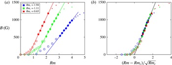
(a) Bifurcation diagram for three values of amplification corresponding to
 $\mathit{Rm}_{c}=1.94$
, 1.11 and 0.65. The saturated regime is marked with filled symbols and fitted using a linear scaling, crossing
 $B=0$
at
 $\mathit{Rm}=\mathit{Rm}_{c}$
. (b) Normalized bifurcation diagram as a function of
 $(\mathit{Rm}-\mathit{Rm}_{c})/\sqrt{\mathit{Rm }_{c}}$
; the linear fit gives a slope of
 $6.6\times 10^{-2}~\text{G}$
in agreement with (3.2).

We focus in this subsection on the Lorentz force saturated regime extending from
 $\mathit{Rm}/\mathit{Rm}_{c}=1.6$
to
 $\mathit{Rm}/\mathit{Rm}_{c}\sim 2.16$
in figure 2(a). As already described in § 3.1, the most probable value of the magnetic field
 $B_{mp}$
is non-zero and the p.d.f. of the magnetic field amplitude and of the magnetic energy display a wide distribution around their mode. This regime is investigated by varying both the rotation rate of the impeller
 $F$
and the amplification factor
 $A$
of the electronic loop (or equivalently the critical magnetic Reynolds number
 $\mathit{Rm}_{c}=(kA)^{-1}$
). Figure 5(a) shows bifurcation diagrams for three critical values, namely
 $\mathit{Rm}_{c}=1.94$
, 1.11 and 0.65. In each case there is a significant range of
 $\mathit{Rm}$
values over which the time-averaged magnetic field grows linearly with the distance to threshold:
 $$\begin{eqnarray}\langle B\rangle \propto (\mathit{Rm}-\mathit{Rm}_{c}),\end{eqnarray}$$
for which the prefactor depends on the amplification factor
 $A$
. We will now show that this scaling can be recovered from the induction equation (2.6) and the feedback constitutive equation (2.7). Let us first discuss the induction equation (2.6) which was expressed in Verhille et al. (Reference Verhille, Khalilov, Plihon, Frick and Pinton2012) as
 $\langle B_{z}\rangle =k\,\mathit{Rm}(1-{\it\alpha}\sqrt{N})\langle B_{x}\rangle$
. In the original expression, the authors used
 $N^{ind}=(B_{x}^{2}{\it\sigma}R_{0})/({\it\rho}U)$
; in our work, we will use the more accurate expression
 $N^{BvK\,onset}=(kB_{x}^{2}{\it\sigma}R_{0})/({\it\rho}U)$
, which takes into account the
 $k$
geometrical factor for a more accurate estimate of the induced current; it is then necessary to replace
 ${\it\alpha}$
by
 ${\it\alpha}/\sqrt{k}$
in the induction law. We showed in § 2 that, close to dynamo onset,
 $N^{BvK\,onset}$
is equivalent to
 $N^{BvK}=B_{x}^{2}/(A{\it\mu}_{0}{\it\rho}U^{2})$
. The strength of the Lorentz force is equivalently taken into account when using both expressions, but more accurately estimated using the relation
 $B_{x}=AB_{z}$
ascribed by the amplification feedback loop than assuming any functional form for the induction law. Close to dynamo onset, we combine the induction law (2.6) and the feedback law (2.7), using the expression of
 $N^{BvK}$
for the interaction parameter, which gives
 $$\begin{eqnarray}\langle B\rangle =\sqrt{\frac{{\it\rho}}{{\it\mu}_{0}}}\frac{1}{{\it\alpha}{\it\sigma}R_{0}}\left(\frac{\mathit{Rm}-\mathit{Rm}_{c}}{\sqrt{\mathit{Rm }_{c}}}\right).\end{eqnarray}$$
This formula brings out that this scaling is independent of the amplification factor when choosing the control parameter
 $(\mathit{Rm}-\mathit{Rm}_{c})/\sqrt{\mathit{Rm }_{c}}$
as the relevant control parameter of the saturated regime. The prefactor only depends on the fluid physical characteristics and on geometric parameters determined empirically; this gives a value of
 $6.2\times 10^{-2}~\text{G}\pm 10\,\%$
with
 ${\it\alpha}=2.73\pm 0.23$
.
A good agreement between the experimental data and the proposed scaling is observed in figure 5(b), when the dynamo field is plotted as a function of
 $(\mathit{Rm}-\mathit{Rm}_{c})/\sqrt{\mathit{Rm }_{c}}$
: in the saturated regime, curves collapse on a single master curve. The black line in figure 5(b) is a least-square fit of the data in the saturated regime for three values of the amplification, with slope
 $6.6\times 10^{-2}~\text{G}$
, within the error given above.
3.4. Power budget
3.4.1. Channels for power dissipation in homogeneous and semi-synthetic dynamos
Precise estimation of the power budget in dynamo regimes is a long-standing issue in dynamo theory. In homogeneous dynamo regimes, dissipation occurs via two channels: viscous dissipation in the fluid flow (denoted as
 $P_{F}$
in the remainder) and Joule dissipation from electrical currents generating the dynamo magnetic field (denoted as
 $P_{J}$
). For natural and experimental dynamos, these two dissipation terms should be estimated from sources of kinetic energy (convection, mechanical stirring, etc.) which are coupled to the magnetic energy.
For instance, for an experimental homogeneous dynamo driven by mechanical stirring, the total dissipated power
 $P_{T}$
is equal to the power delivered by the stirring system, denoted
 $P_{M}$
, and the power balance reads
 $$\begin{eqnarray}P_{T}=P_{M}=P_{F}+P_{J}\quad (\text{homogeneous dynamo}).\end{eqnarray}$$
In these homogeneous systems (which can be seen as isolated systems), the only directly measurable power is
 $P_{M}$
.
On the other hand, semi-synthetic dynamos, such as the Bullard–von Kármán set-up are more complex: they can be analysed as open or isolated systems depending on which energy sources are considered. They can be seen as open systems when taking into account only the mechanical power
 $P_{M}$
or as isolated systems when considering both the mechanical power
 $P_{M}$
and the contribution of the power supply feeding the coils
 $P_{PS}=RI^{2}$
. A global power budget of the isolated system is then
 $$\begin{eqnarray}P_{T}=P_{M}+P_{PS}=P_{F}+P_{J}+P_{PS}\quad (\text{semi-synthetic dynamo}).\end{eqnarray}$$
One asset of the Bullard–von Kármán set-up, when considering only the mechanical power (and thus an open system), is that the dynamo may be switched off (on) at will by opening (closing) the feedback loop, giving access to the mechanical power for two distinct flow regimes driven by the same rotation rate
 $F$
of the impellers (one being an hydrodynamic regime, the other being an MHD regime). In the following subsection, we will first investigate the modification of mechanical power between hydrodynamic regimes (in the open-loop, dynamo-free, configuration) and MHD (or dynamo) regimes, then focus on the global power budget.
3.4.2. Mechanical power dissipation
Let us first focus on the injected mechanical power
 $P_{M}$
required to sustain a given rotation of the impellers
 $F=\mathit{Rm}/({\it\mu}{\it\sigma}2{\rm\pi}R_{0}^{2})$
. Due to the two dissipation channels from mechanical power,
 $P_{M}=P_{F}+P_{J}$
, the natural variables for the power dissipation terms are
 $\mathit{Rm}$
(accounting for the intensity of turbulence) and
 $B$
(accounting for the intensity of the Joule dissipation at a given value of
 $\mathit{Rm}$
). The mechanical power is computed as
 $P_{M}=2{\rm\pi}F{\it\Gamma}$
with the mechanical torque
 ${\it\Gamma}=K_{{\it\Gamma}}I_{mot}$
computed from the measurement of current consumption of the motor drives
 $I_{mot}$
, with
 $K_{{\it\Gamma}}$
a motor-specific factor.
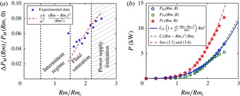
(a) Normalized power difference
 ${\rm\Delta}P_{M}(\mathit{Rm})/P_{M}(\mathit{Rm},0)$
as a function of
 $\mathit{Rm}/\mathit{Rm}_{c}$
, see text for details. (b) Evolution of the time-averaged mechanical power (
 $\langle P_{M}(\mathit{Rm},B)\rangle$
, circles), electric power injected through the coils (
 $R\langle I\rangle ^{2}$
, squares) and the total power (
 $\langle P_{T}\rangle$
, stars) as a function of
 $\mathit{Rm}/\mathit{Rm}_{c}$
for
 $\mathit{Rm}_{c}=1.94$
. The lines corresponds to the scalings given by (3.7) (solid) and (3.8) (dashed) and a combination of the two (dash-dotted).

In the absence of external feedback, which will be referred to as the ‘open-loop’ configuration, the only channel is viscous dissipation (hydrodynamic flow), and
 $P_{M}(\mathit{Rm},B=0)=P_{F}(\mathit{Rm},0)$
; this is also valid below dynamo onset. In dynamo regimes (MHD flow),
 $P_{M}(\mathit{Rm},B)=P_{F}(\mathit{Rm},B)+P_{J}(\mathit{Rm},B)$
, where
 $B$
depends on
 $\mathit{Rm}$
through the dynamo scaling law (note that
 $P_{F}(\mathit{Rm},B)$
is the power required to sustain the flow modified by the Lorentz forces, not taking into account the Joule dissipation, and that
 $\mathit{Rm}$
is based on the tip velocity of the impellers and not the actual flow velocity in the MHD regime). As previously pointed out, we have access to the difference between mechanical power in the BvK dynamo configuration and in the ‘open-loop’ configuration,
 ${\rm\Delta}P_{M}(\mathit{Rm})=P_{M}(\mathit{Rm},B)-P_{M}(\mathit{Rm},0)$
, for a given value of
 $\mathit{Rm}$
. The normalized mechanical power difference
 ${\rm\Delta}P_{M}(\mathit{Rm})/P_{M}(\mathit{Rm},0)$
is displayed in figure 6(a). A clear increase of the mechanical power consumption of a few per cent is observed in regimes where saturation of the BvK dynamo occurs through Lorentz force modification of the bulk flow. This increase can be understood following the previous study in Verhille et al. (Reference Verhille, Khalilov, Plihon, Frick and Pinton2012), which showed, in induction regimes, that the mechanical power in the MHD case,
 $P_{M}(\mathit{Rm},B)$
, is related to the mechanical power in the hydrodynamic regime,
 $P_{M}(\mathit{Rm},0)$
, as
 $$\begin{eqnarray}P_{M}(\mathit{Rm},B)=(1+{\it\gamma}N^{ind})P_{M}(\mathit{Rm},0)\end{eqnarray}$$
with
 ${\it\gamma}=140$
an empirical constant. We previously showed that close to dynamo onset, the scaling laws determined from induction measurements remain valid using
 $N^{BvK}$
. Accordingly,
 ${\rm\Delta}P_{M}(\mathit{Rm})/P_{M}(\mathit{Rm},0)={\it\gamma}N$
, and
 $N$
can be recast using the dynamo scaling law (3.2). The expected evolution
 $$\begin{eqnarray}{\rm\Delta}P_{M}(\mathit{Rm})/P_{M}(\mathit{Rm},0)=\frac{{\it\gamma}k}{{\it\alpha}^{2}}\frac{(\mathit{Rm}-\mathit{Rm}_{c})^{2}}{\mathit{Rm}^{2}}\end{eqnarray}$$
is displayed in figure 6(a) as a dashed line and shows good agreement with experimental data. The open circles symbols in figure 6(b) display the evolution of the time-average injected mechanical power as a function of
 $\mathit{Rm}$
, for
 $\mathit{Rm}_{c}=1.94$
. These points can be compared to the scaling of (3.5), using both the dynamo scaling law (3.2) and the turbulent scaling of the hydrodynamic regime
 $P_{M}(\mathit{Rm},0)=2K_{p}{\it\rho}/({\it\mu}^{3}{\it\sigma}^{3}R_{0})\mathit{Rm}^{3}$
, following the notation of Ravelet et al. (Reference Ravelet, Chiffaudel, Daviaud and Léorat2005), which gives
 $$\begin{eqnarray}P_{M}(\mathit{Rm},B)=\frac{2K_{p}{\it\rho}}{{\it\mu}^{3}{\it\sigma}^{3}R_{0}}\left(1+\frac{{\it\gamma}k}{{\it\alpha}^{2}}\frac{(\mathit{Rm}-\mathit{Rm}_{c})^{2}}{\mathit{Rm}^{2}}\right)\mathit{Rm}^{3},\end{eqnarray}$$
where the power is expressed in kW, and
 ${\it\gamma}=140$
and
 $K_{p}=5.03\times 10^{-2}$
(a value similar to the value
 $6.1\times 10^{-2}$
reported by Ravelet et al.
Reference Ravelet, Chiffaudel, Daviaud and Léorat2005 in a similar water flow). The good agreement between experimental data and (3.7) shows once again the consistency of our results and that the features of the BvK dynamo can be fully understood from the effect of Lorentz forces in the MHD regime.
 ${\rm\Delta}P_{M}(\mathit{Rm})$
is linked to modifications of viscous dissipation between the hydrodynamic regime and the MHD regime (
 ${\rm\Delta}P_{F}$
) and to the occurrence of Joule dissipation
 $P_{J}$
. While Joule dissipation obviously increases the mechanical power, the sign of
 ${\rm\Delta}P_{F}=P_{F}(\mathit{Rm},0)-P_{F}(\mathit{Rm},B)$
cannot be easily estimated. The modifications of viscous dissipation could thus lead to both an increase or a decrease of the mechanical power (depending on the details of the flow modifications at saturation). A precise estimate of the ratio of the two dissipation channels is thus outside the scope of the present study and would require precise measurements of the velocity field and current density. We emphasize here that, investigating only the modification of the injected mechanical power, one considers the Bullard–von Kármán dynamo as an open system. Extrapolations to homogeneous dynamos, seen as isolated systems, should thus be done with care.
3.4.3. Global power budget
Let us now consider the Bullard–von Kármán dynamo as an isolated system and investigate the total injected power
 $P_{T}=P_{M}+P_{PS}$
. While for an homogeneous dynamo
 $P_{J}$
accounts for the power required to sustain the dynamo magnetic field, in semi-synthetic dynamos the power required to sustain the dynamo magnetic field is provided by an external power supply and
 $P_{PS}=RI^{2}$
(where
 $R$
is the resistance of the coils). Note that the feedback to the induced magnetic field by the flow in the coils is neglected since
 $\mathit{Rm}^{eff}=B_{z}/B_{x}$
remains small and the power supply is current-controlled. In these cases,
 $P_{PS}$
is not universal and is system-dependent through its dependence on
 $R$
(and thus the way the system is being built). However, since the electrical current in the coils is proportional to the dynamo magnetic field
 $B$
,
 $P_{PS}$
is proportional to the Joule dissipated power. A precise estimate of
 $P_{J}$
would require the measurement of the current at each location in space, which is outside the scope of the present work. However, an estimation of the Joule power dissipation
 $P_{J}^{e}$
can be made from the measurement of the magnetic field at one location using
 $|\boldsymbol{j}|=|\boldsymbol{{\rm\nabla}}\times \boldsymbol{B}_{\boldsymbol{z}}/{\it\mu}_{0}|\sim B_{x}/({\it\mu}_{0}AR_{0})$
. Consequently,
 $P_{J}^{e}\sim (B^{2}R_{0}/{\it\mu}_{0}^{2}{\it\sigma}A^{2})$
(recall that
 $B=B_{x}$
).
It thus follows that
 $P_{PS}={\it\chi}A^{2}P_{J}^{e}$
, with
 ${\it\chi}$
a non-universal constant (depending on geometrical factors and the resistivity of the external coils). The
 $A^{2}$
is reminiscent of the external amplification loop: for a given value of induced magnetic field in the fluid volume, the dynamo magnetic field is
 $A$
-fold larger; the power needed to sustain the dynamo is thus a factor
 $A^{2}$
larger than the estimated Joule dissipated power in the flow volume. The experimental evolution of the power delivered by the external power supply
 $P_{PS}$
as a function of
 $\mathit{Rm}$
, for
 $\mathit{Rm}_{c}=1.94$
, is displayed as square symbols in figure 6(b). The experimental points are correctly described in the regime of Lorentz force saturation using the dynamo scaling law (3.2) for the estimate of
 $P_{PS}$
:
 $$\begin{eqnarray}P_{PS}=C_{I}\frac{(\mathit{Rm}-\mathit{Rm}_{c})^{2}}{\mathit{Rm}_{c}},\end{eqnarray}$$
with formula:
 $C_{I}=(R{\it\kappa}^{2}{\it\rho})/({\it\mu}_{0}{\it\sigma}^{2}{\it\alpha}^{2}R_{0})=1.52$
(with
 $R=0.28~{\rm\Omega}$
) and
 $P_{PS}$
expressed in kW, which is displayed as a dashed line in figure 6(b). It should be noted that a departure from the expected scaling is observed for
 $\mathit{Rm}/\mathit{Rm}_{c}$
values above 2.16, due to power limit saturation, as already discussed in § 3.1. Finally, the experimental data for the total injected power
 $P_{T}=P_{M}+P_{PS}$
are also displayed in figure 6(b) as stars. These points are described to a very good accuracy by the scaling law given by the sum of (3.7) and (3.8) and displayed as a dash-dotted line in figure 6(b). Finally, the
 $A^{2}$
factor in
 $P_{PS}$
can be understood as a way to control the ratio
 $P_{M}/P_{PS}$
in the Lorentz force saturation regime. For
 $\mathit{Rm}_{c}=(kA)^{-1}=1.94$
, the electrical power required to sustain the dynamo is roughly equal to the injected mechanical power in the saturated regime. As the critical magnetic Reynolds number is reduced,
 $P_{PS}$
becomes 2.3 times larger than
 $P_{M}$
for
 $\mathit{Rm}_{c}=1.11$
and 9 times larger for
 $\mathit{Rm}_{c}=0.65$
. We emphasize that these numbers should be taken with care since they depend on the value of
 ${\it\chi}$
and thus on the design of the system (using superconductive coils would for instance strongly decrease
 $P_{PS}$
for the same value of the dynamo magnetic field).
4. Dynamics of dynamo polarity inversions
Polarity inversions of the dynamo magnetic field are expected because the system is invariant under the
 $(\boldsymbol{B}\rightarrow -\boldsymbol{B})$
symmetry. Reversals of the dynamo field have been observed in paleomagnetic recording of the Earth dynamo field (Valet, Meynadier & Guyodo Reference Valet, Meynadier and Guyodo2005) as well as in experimental VKS dynamos (Berhanu et al.
Reference Berhanu, Monchaux, Fauve, Mordant, Pétrélis, Chiffaudel, Daviaud, Dubrulle, Marié, Ravelet, Bourgoin, Odier, Pinton and Volk2007); in this last case, dynamical regimes are controlled by the coupling between turbulent flows and magnetic modes. In the BvK experiment, two polarities are accessible since the power supply feeding the coils is bipolar. Polarity inversions are not associated with hydrodynamic transitions, and have already been observed in the kinematic BvK configuration detailed in Verhille et al. (Reference Verhille, Plihon, Fanjat, Volk, Bourgoin and Pinton2010). (In the previous kinematic studies, inversions were much harder to observe due to the presence of ferromagnetic pieces close to each motor: their remnant magnetic field of about 0.1 G in the bulk of the gallium flow was sufficient to break the (
 $B\rightarrow -B$
) symmetry of the system.) They require the presence of additive noise (such as magnetic field of the Earth and/or electronic noise), such that, when the dynamo field decreases close to zero amplitude due to multiplicative noise, the system can be pushed towards the fixed point with other polarity.
In the case considered here, where the field saturates due to the action of Lorentz forces, polarity inversions have been shown in figure 2(c). The frequency of the inversions drops rapidly as
 $\mathit{Rm}/\mathit{Rm}_{c}$
increases: excursions to
 $B\sim 0$
become less frequent, and thus inversions occur less frequently. Consequently, statistical analysis of these inversions is limited to moderate values of
 $\mathit{Rm}/\mathit{Rm}_{c}$
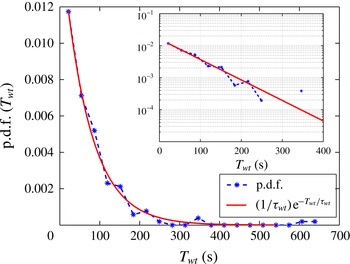
. Figure 7 shows the probability distribution function of the time interval between two inversions for
 $\mathit{Rm}/\mathit{Rm}_{c}=1.66$
. These time intervals obey a Poisson process, with mean interval time
 ${\it\tau}_{wt}=67~\text{s}$
, as given by the best fit of the experimental data with the functional form
 $(1/{\it\tau}_{wt})\,\text{exp}(-T_{wt}/{\it\tau}_{wt})$
shown in figure 7. Note that, due to slow variations of the additive noise, the time recordings of regimes displaying inversions is limited to 18 000 s. This limits the number of recorded events to 350 samples, and the accuracy of the p.d.f. for the longer and less frequent events.
Distribution of waiting time between two successive polarity inversions at
 $\mathit{Rm}/\mathit{Rm}_{c}=1.66$
. Inset: same plot in lin-log scale. The solid line is a fit of the form
 $1/{\it\tau}_{wt}\,\text{exp}\,(-T_{wt}/{\it\tau}_{wt})$
with best fit given for
 ${\it\tau}_{wt}=67~\text{s}$
.

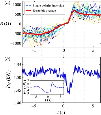
We will now investigate in greater detail the dynamics of individual inversions. Figure 8(a) shows individual time series of magnetic field inversions, as well as the time-averaged behaviour of 123 independent events displayed by the thick solid line (each inversion has been shifted such that
 $t=0~\text{s}$
corresponds to the time when the ensemble average is crossing
 $B=0$
and
 $t=0.8~\text{s}$
is the beginning of the growth of the dynamo field from zero). Although individual events display turbulent fluctuations, the average behaviour has a well-defined pattern. For
 $t<0$
, the field decreases slowly from its saturated value to
 $B=0$
. The magnetic field remains null during a time interval varying from 0.1 to
 $5~\text{s}$
depending on the considered event. A growing phase where
 $B$
increases much faster that its decay (the growth phase is in fact limited by the slew rate of the power supply:
 $150~\text{A}~\text{s}^{-1}$
or equivalently
 $1200~\text{G}~\text{s}^{-1}$
) then follows. The dynamo field displays a short overshoot before reaching its saturated value in the positive polarity. This typical behaviour, also observed in the VKS dynamo (Berhanu et al.
Reference Berhanu, Monchaux, Fauve, Mordant, Pétrélis, Chiffaudel, Daviaud, Dubrulle, Marié, Ravelet, Bourgoin, Odier, Pinton and Volk2007), has been detected for all
 $\mathit{Rm}/\mathit{Rm}_{c}$
values in the range
 $[0.74;1.66]$
.
Let us now focus on the time-averaged total power consumption during inversions. Figure 8(b) shows an ensemble average of
 $P_{M}$
over 123 inversions for
 $\mathit{Rm}/\mathit{Rm}_{c}=1.66$
. In the Lorentz force saturated regimes (in both polarities), the mechanical injected power
 $P_{M}$
is of the order of 1.53 kW at
 $\mathit{Rm}/\mathit{Rm}_{c}=1.66$
(see figure 8
b). Following the dynamics of the reversal, the mechanical power first decreases to 1.44 kW, which represents the turbulent dissipation to sustain the hydrodynamic flow (when
 $B=0$
), and then increases again to its initial value after a slight overshoot. The 60 W decrease of
 $P_{M}$
can only be observed in the ensemble average over several realizations due to turbulent fluctuations (non-coherent turbulent fluctuations are of the order of 200 W). It is interesting to look at the ensemble average of the total power consumption
 $P_{T}$
during polarity inversions (see inset of the figure 8
b). The overshoot observed on the dynamo field is also present on the total injected power, which reaches 6.5 kW, i.e. a 75 % increase of the magnetic power as compared to the saturated regimes. The magnetic field growth is maintained by favourable velocity gradients in the flow, which are then reduced due to the action of the Lorentz forces in the saturated regime. The presence of the overshoot demonstrates the delay required for the Lorentz forces to reorganize the velocity gradients from the hydrodynamic regime to the MHD (or Lorentz force saturation) regime.
(a) Time series of a single inversion (dashed lines) and ensemble average over 123 events (thick solid line) for
 $\mathit{Rm}/\mathit{Rm}_{c}=1.66$
;
 $t=0$
corresponds to the time when the ensemble average crosses
 $B=0$
and
 $t=0.8~\text{s}$
to the start of the growth in the other polarity. (b) Ensemble average of the mechanical power
 $P_{M}$
during polarity inversions at total injected power at
 $\mathit{Rm}/\mathit{Rm}_{c}=1.66$
(and
 $\mathit{Rm}_{c}=2.4$
). Inset: ensemble average of the total power
 $P_{T}=P_{M}+P_{PS}$
during polarity inversions.

5. From self-killing to subcritical dynamos
In previous sections, we have investigated the features and the dynamics of supercritical dynamo regimes of the semi-synthetic BvK dynamo. In particular, we showed a transition from an hydrodynamic base flow below dynamo onset (i.e. a solution of the Navier–Stokes equation without the Lorentz force term) to an MHD flow (for which the Lorentz force term becomes a dominant player in the Navier–Stokes equation). The versatile nature of the semi-synthetic set-up also allows us to explore other dynamo regimes: (i) self-killing dynamos for which the hydrodynamic base flow sustains the growth of a dynamo, but the MHD flow (reached when the dynamo field is strong enough) does not sustain a dynamo, (ii) subcritical dynamos for which the dynamo instability can only be reached from an MHD base flow (i.e. in the presence of an initial strong magnetic field). In this section, we will explore experimentally these regimes, focusing on the subcritical regime. Although somewhat preliminary, these results are included here, because subcriticality of the dynamo instability is a feature often conjectured for astrophysical bodies. It has been proposed for the Martian dynamo (Kuang, Jiang & Wang Reference Kuang, Jiang and Wang2008), Keplerian flows (Rincon, Ogilvie & Proctor Reference Rincon, Ogilvie and Proctor2007), spherical rotating convective states (Sreenivasan & Jones Reference Sreenivasan and Jones2011), in numerical simulations of Taylor–Green flows (Ponty et al.
Reference Ponty, Laval, Dubrulle, Daviaud and Pinton2007), or of von Kármán flows (Reuter, Jenko & Forest Reference Reuter, Jenko and Forest2009), but also in experiments (Miralles et al.
Reference Miralles, Herault, Fauve, Gissinger, Pétrélis, Daviaud, Dubrulle, Boisson, Bourgoin, Verhille, Odier, Pinton and Plihon2014). Subcritical behaviour in numerical simulations can be observed from a saturated self-excited regime (
 $\mathit{Rm}>\mathit{Rm}_{c}$
) and suddenly decreasing
 $\mathit{Rm}$
as in Ponty et al. (Reference Ponty, Laval, Dubrulle, Daviaud and Pinton2007) and Sreenivasan & Jones (Reference Sreenivasan and Jones2011). They can also be obtained when applying an external magnetic field at
 $\mathit{Rm}<\mathit{Rm}_{c}$
and suddenly switching it off as reported in Reuter et al. (Reference Reuter, Jenko and Forest2009) for a spherical von Kármán flow. We will follow a similar idea here: the experimental arrangement is set such that the dynamo instability is observed from an initial MHD base flow, while no dynamo excitation is possible from an initial hydrodynamic base flow. Note that, since the MHD flow is the saturated velocity field of the supercritical dynamos, this experimental strategy is very similar to the one implemented numerically in Cattaneo & Tobias (Reference Cattaneo and Tobias2009). In this study, the authors, using kinematic computations, found positive dynamo growth rates for the velocity field of a saturated dynamo configuration (when solving the coupled problem). Here, this arrangement is made possible since the semi-synthetic dynamo features depend on (i) the characteristics of the external loop, (ii) the details of the turbulent induction process measured by the internal magnetic sensor.
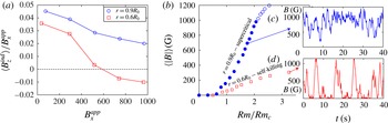
(a) Time-averaged induction profile (open loop configuration) with constant applied field
 $B_{x}^{app}$
up to 1000 G for two depths of the magnetic sensor at
 $\mathit{Rm}=3.7$
. The sign of the induced field changes at
 $r=0.6R_{0}$
for large applied field whereas it remains positive for
 $r=0.9R_{0}$
for every amplitude of the applied field. (b) Bifurcation diagram for the two locations, for a positive amplification factor
 $A>0$
. Circles: supercritical bifurcation already described in § 3; squares: self-killing dynamo. (c,d) Time series of the BvK fields for the two types of dynamos.

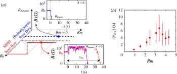
(a) Schematic bifurcations for a negative amplification factor
 $A<0$
and a magnetic sensor located at
 $r=0.6R_{0}$
as a function of the amplitude of the applied field
 $B_{0}$
(which is switched off at
 $t=0$
). The blue dashed line stands for
 $B_{0}<600~\text{G}$
, too weak to modify significantly the flow. The red line represents a subcritical bifurcation, obtained when the applied magnetic field at
 $t<0$
is large enough to achieve an MHD flow. The time series (
 $\mathit{Rm}=3$
) correspond to the two cases. (b) Averaged life-time of the subcritical dynamo as a function of
 $\mathit{Rm}$
. Error bars represent standard deviations.

Measurements reported so far have been performed with the magnetic probe located in the mid-plane of the cylinder at
 $r=0.9R_{0}$
. At this location, for all amplitudes of an imposed external magnetic field
 $B_{x}$
, the induced field
 $B_{z}$
is always positive as shown in figure 9(a) (in the open-loop configuration). The supercritical dynamo regimes described in the previous sections are observed from an initial hydrodynamic base flow when the amplification factor
 $A$
is positive (when the feedback loop is closed), as reproduced in figure 9(b) (filled circles) and with a typical time series displayed in figure 9(c). The situation drastically changes if the magnetic probe is located at
 $r=0.6R_{0}$
: in the open-loop configuration the amplitude of the axial induced magnetic field changes sign for
 $B_{x}>600~\text{G}$
. If the amplification factor
 $A$
of the feedback loop is positive, dynamo action will be excited from the initial hydrodynamic base flow (for
 $\mathit{Rm}>\mathit{Rm}_{c}$
). But as the amplitude of the dynamo field
 $B_{x}$
grows, the MHD flow does not favour a dynamo any longer. The resulting behaviour is that of a ‘self-killing’ dynamo (Fuchs, Rädler & Rheinhard Reference Fuchs, Rädler and Rheinhard1999), where the action of the Lorentz force from the dynamo magnetic field kills the dynamo as shown in figure 9(d). The corresponding bifurcation is shown as square symbols in figure 9(b).
For a negative amplification factor
 $A$
, subcritical dynamo regimes can be observed. In this configuration, while the hydrodynamic base flow is always stable (i.e. no dynamo can be excited), the MHD base flow may be able to sustain a dynamo if
 $\mathit{Rm}$
is above a critical value. The MHD base flow being obtained in the presence of a strong
 $B_{x}$
field, we thus excite a subcritical dynamo regime. The experimental protocol is the following: (i) we apply a large constant magnetic field
 $B_{0}$
to reach the MHD base flow in the open-loop configuration; (ii) then, simultaneously, and at time
 $t=0$
the applied field is switched off and the BvK feedback-loop is turned on. Figure 10(a) displays a schematic three-dimensional plot of the evolution of the subcritical dynamo magnetic field as a function of
 $\mathit{Rm}$
and of the amplitude of the initial external field
 $B_{0}$
(applied at
 $t<0$
). When
 $B_{0}$
is lower than 600 G (blue solid line), the base flow is hydrodynamic and
 $B=0$
is the stable fixed point of the BvK loop with
 $A<0$
. As a consequence, the magnetic field decays rapidly to
 $B=0$
for
 $t>0$
(as shown in the time series of the upper panel of figure 10
a). For
 $B_{0}$
and
 $\mathit{Rm}$
sufficiently large, a dynamo field can be maintained for some time.
Time series of two independent realizations are shown in the bottom panel of figure 10(a). The dynamo field is observed for
 ${\sim}20~\text{s}$
and
 ${\sim}40~\text{s}$
for these two realizations. We note that the value of the subcritical dynamo field is around the maximum achievable magnetic field value (1200 G), and does not depend on the magnitude of the initial applied constant magnetic field. The dynamo field may be larger than the initial applied magnetic field as observed in numerical studies (Tilgner & Brandenburg Reference Tilgner and Brandenburg2008). Due to the limitation of available coil current, the subcritical dynamo regimes observed here are limited to the ‘kinematic phase’, since no modification of the initial MHD base flow is currently achievable with our power supply. These subcritical dynamo regimes thus have a finite life-time since, eventually, turbulent fluctuations may be large enough to decrease the dynamo field such that the flow will bifurcate to a hydrodynamic flow, for which
 $B=0$
is a stable fixed point. The dynamo life-time is observed to vary from 0 to 100 s. The evolution of the average life-time of the dynamo state with
 $\mathit{Rm}$
is shown in figure 10(b), where the error bars represent the standard deviation. The average dynamo life-time increases when
 $\mathit{Rm}$
increases from 0 to 3.5 and decreases above 3.5 due to the increase of turbulent fluctuations driving the system back to
 $B=0$
. This complex configuration and its associated dynamics are still under investigation.
6. Discussion and conclusion
We have reported several features from a versatile semi-synthetic dynamo set-up built combining a turbulent induction process (from a von Kármán liquid gallium flow) and an electronic feedback: the Bullard–von Kármán (BvK) dynamo. This semi-synthetic turbulent dynamo has a critical magnetic Reynolds number of order unity and we have focused on regimes where saturation occurs via a modification of the bulk flow by the action of Lorentz forces. Following the results given by kinematic studies showing that the most unstable magnetic mode of a von Kármán flow is an equatorial dipole (Ravelet et al. Reference Ravelet, Chiffaudel, Daviaud and Léorat2005; Stefani et al. Reference Stefani, Xu, Gerbeth, Ravelet, Chiffaudel, Daviaud and Léorat2006), this article focuses on regimes of the BvK dynamo with an equatorial dipole dynamo mode which is imposed by the configuration of the external coils.
The simplest configuration consists of a supercritical dynamo instability. Its main feature is that below dynamo onset, the base flow is purely hydrodynamic (i.e. a solution of the Navier–Stokes equation without the Lorentz force term), while above onset the flow becomes MHD (i.e. strongly affected by the back reaction of Lorentz forces). The critical value of the magnetic Reynolds number of the instability is set arbitrarily by tuning the amplification factor of the electronic loop. Increasing this value decreases
 $\mathit{Rm}_{c}$
and increases the interaction parameter
 $N$
, a proxy of the effect of the magnetic field on the flow. The bifurcation occurs through bursts of magnetic field characteristic of on–off intermittency. We report for the first time the scaling law of the BvK dynamo in the Lorentz force bulk saturation regime, where the magnetic field is observed to scale as
 $\mathit{Rm}-\mathit{Rm}_{c}$
. The polarity inversions, for which the statistics of waiting time between two events follows a Poisson’s law, are a good way to probe the modification of the flow by the Lorentz forces. During these inversions, the system alternates between MHD flow regimes and hydrodynamic regimes (
 $B=0$
). We showed that, during these inversions, drastic changes in injected power are recorded, contrary to other experimental dynamos displaying similar magnetic reversals.
We also reported the existence of self-killing and subcritical regimes when modifying either the details of the turbulent induction process or the properties of the amplification feedback.
One of the asset of the BvK dynamo is that a global effect of Lorentz forces on the flow is observed at saturation. In the regimes studied previously, the injected mechanical power increases by 5–8 % in the dynamo state as compared to the hydrodynamic state and that this increase scales as
 ${\rm\Delta}P_{M}/P_{M}\propto (\mathit{Rm}-\mathit{Rm}_{c})^{2}/\mathit{Rm}^{2}$
. We infer that this amount depends on the configuration of the flow and the geometry of the magnetic field. Previous work with constant applied transverse field (Verhille et al.
Reference Verhille, Khalilov, Plihon, Frick and Pinton2012) showed that we could expect a 50 % increase for other flow configurations (for instance by rotating only one impeller or driving both impellers in the same direction). Following these results, we suggest that similar semi-synthetic dynamos configurations could display
 ${\rm\Delta}P_{M}=0$
or even
 ${\rm\Delta}P_{M}<0$
for specific base flow, meaning that driving the dynamo saturated flow may require less mechanical power than driving the hydrodynamic base flow. In the present configuration,
 ${\rm\Delta}P_{M}$
is a few per cent of the turbulent dissipation, a level easily measured. When taking into account the electrical power required to sustain the dynamo magnetic field, the increase of total injected power exceeds 50 %. This is an important feature of the Bullard–von Kármán dynamo; in particular no measurable changes in injected mechanical power were observed in the VKS experiment. Regarding the results detailed in this article, this is a very peculiar feature of the VKS experiment. It should be noted that the scalings reported for the BvK dynamo are difficult to extrapolate to homogeneous dynamos since they depend on the amplification factor
 $A$
. Precise comparison would require detailed velocity measurements. So far, in the BvK set-up we have been able to measure mean velocity profiles with ultrasound Doppler velocimetry (Takeda Reference Takeda1995; Aubert et al.
Reference Aubert, Brito, Nataf, Cardin and Masson2001) for very low rotation rate of the disks. It has been observed that the shape of the profile
 $v_{x}$
(aligned with the dynamo field) does not evolve when the dynamo is present, while the sign of
 $v_{y}$
(transverse to the main direction of the magnetic field) is reversed for large magnetic fields. On the contrary, in the VKS experiment no modifications of the velocity signal measured using a potential probe in the mid-plane were observed above dynamo onset.
Acknowledgements
We acknowledge the technical support of M. Moulin. This work has been supported by contract ANR-08-BLAN-0039-02. S.M. is supported by ERC grant 247303 (MFECE) of A. Jackson (ETH Zürich).