3.1. Derivation based on the wave equation for Lagrangian pressure perturbations

We search for a solution to (2.9) in the form

(3.3) $$\begin{eqnarray}\tilde{p}(z)=\tilde{p}(0)\exp \left(\text{i}L\int _{0}^{{\it\zeta}}{\it\varphi}({\it\zeta}_{1},L)\,\text{d}{\it\zeta}_{1}\right),\quad {\it\zeta}=z/L,\end{eqnarray}$$

where ${\it\varphi}$ is an unknown function of the dimensionless variable ${\it\zeta}$ and the parameter $L$ . In a fluid with the background density profile (3.1), substitution of (3.3) into the wave equation (2.9) gives a nonlinear first-order ordinary differential equation (more specifically, a Riccati equation):

(3.4) $$\begin{eqnarray}\frac{\text{i}}{L}\frac{\text{d}{\it\varphi}}{\text{d}{\it\zeta}}+\text{i}{\it\varphi}\left[\frac{1}{h}+\frac{1}{L}\frac{\text{d}}{\text{d}{\it\zeta}}\ln \left(\frac{{\it\omega}_{d}^{2}h}{{\it\omega}_{d}^{4}-g^{2}k^{2}}\right)\right]={\it\varphi}^{2}-m^{2}-\frac{1}{4h^{2}}-\frac{gk^{2}}{L{\it\omega}_{d}^{2}}\frac{\text{d}}{\text{d}{\it\zeta}}\ln \left(\frac{h}{{\it\omega}_{d}^{4}-g^{2}k^{2}}\right),\end{eqnarray}$$

where

(3.5) $$\begin{eqnarray}m^{2}=\frac{{\it\omega}_{d}^{2}}{c^{2}}-k^{2}-\frac{1}{4h^{2}}+\frac{gk^{2}}{{\it\omega}_{d}^{2}}\left(\frac{1}{h}-\frac{g}{c^{2}}\right).\end{eqnarray}$$

Note that $m({\it\zeta})=O(1)$ and does not contain terms that are small or large with respect to the parameter $L$ . For definiteness, it will be implied that $m=|m|$ , when $m^{2}\geqslant 0$ , and $m=\text{i}|m|$ , when $m^{2}<0$ .

We represent the unknown function ${\it\varphi}$ in terms of a power series:

(3.6) $$\begin{eqnarray}{\it\varphi}({\it\zeta},L)=f+\text{i}/2h,\quad f=\mathop{\sum }_{n=0}^{\infty }f_{n}({\it\zeta})L^{-n}\end{eqnarray}$$

in the small parameter of the problem, $L^{-1}$ , and note that

(3.7) $$\begin{eqnarray}f^{2}=\mathop{\sum }_{n=0}^{\infty }L^{-n}\mathop{\sum }_{l=0}^{n}f_{n-l}\,f_{l}=f_{0}^{2}+\mathop{\sum }_{n=1}^{\infty }L^{-n}\left(2f_{0}\,f_{n}+\mathop{\sum }_{l=1}^{n-1}f_{n-l}f_{l}\right).\end{eqnarray}$$

By substituting (3.6) and (3.7) into the Riccati equation (3.4), and equating terms of the same order in $L^{-1}$ , we find

(3.8) $$\begin{eqnarray}\displaystyle & f_{0}=\pm m, & \displaystyle\end{eqnarray}$$

(3.9) $$\begin{eqnarray}\displaystyle & \displaystyle f_{1}=\frac{\text{i}}{2}\frac{\text{d}}{\text{d}{\it\zeta}}\ln \left(\frac{{\it\omega}_{d}^{2}hf_{0}}{{\it\omega}_{d}^{4}-g^{2}k^{2}}\right)+\frac{gk^{2}}{2f_{0}{\it\omega}_{d}^{2}}\frac{\text{d}}{\text{d}{\it\zeta}}\ln \left(\frac{h}{{\it\omega}_{d}^{4}-g^{2}k^{2}}\right)+\frac{1}{4f_{0}h}\frac{\text{d}}{\text{d}{\it\zeta}}\ln \left(\frac{{\it\omega}_{d}^{4}-g^{2}k^{2}}{{\it\omega}_{d}^{2}}\right), & \displaystyle \nonumber\\ \displaystyle & & \displaystyle\end{eqnarray}$$

(3.10) $$\begin{eqnarray}\displaystyle & \displaystyle f_{n}=\frac{1}{2f_{0}}\left[\text{i}f_{n-1}\frac{\text{d}}{\text{d}{\it\zeta}}\ln \left(\frac{{\it\omega}_{d}^{2}hf_{n-1}}{{\it\omega}_{d}^{4}-g^{2}k^{2}}\right)-\mathop{\sum }_{l=1}^{n-1}f_{l}\,f_{n-l}\right],\quad n\geqslant 2. & \displaystyle\end{eqnarray}$$

$m\neq 0$

${\it\omega}_{d}\neq 0$

${\it\omega}_{d}^{2}\neq gk$

(3.11) $$\begin{eqnarray}m^{2}+\left(\frac{1}{2h}-\frac{gk^{2}}{{\it\omega}_{d}^{2}}\right)^{2}=\left(1-\frac{g^{2}k^{2}}{{\it\omega}_{d}^{4}}\right)\left(\frac{{\it\omega}_{d}^{2}}{c^{2}}-k^{2}\right)\end{eqnarray}$$

it follows that all $f_{n}$ are finite when $0<m^{2}<\infty$ .

When $m\neq 0$ , the solutions (3.3) corresponding to the upper and lower signs in (3.8) are linearly independent, and (3.6), (3.8)–(3.10) define the full asymptotic solution of the problem. This is the WKB asymptotic solution for AGWs. The solution breaks down in the vicinity of a point or points where $m=0$ . Such points are referred to as turning points (Brekhovskikh & Godin Reference Brekhovskikh and Godin1998).

WKB approximations of various order are obtained by retaining a finite number of terms in the series (3.6). In the first WKB approximation, one retains only terms $f_{0}$ and $f_{1}$ . Then, (3.6), (3.8) and (3.9) give two linearly independent approximate solutions of the wave equation:

(3.12) $$\begin{eqnarray}\displaystyle & \displaystyle \tilde{p}(z)=\tilde{p}(0)\sqrt{\frac{{\it\rho}m(0)({\it\omega}_{d}^{2}-g^{2}k^{2}/{\it\omega}_{d}^{2})}{{\it\rho}(0)m[{\it\omega}_{d}^{2}(0)-g^{2}k^{2}/{\it\omega}_{d}^{2}(0)]}}\exp \left(\pm \text{i}\left(\int _{0}^{z}m\,\text{d}z_{1}+{\it\chi}\right)\right), & \displaystyle\end{eqnarray}$$

(3.13) $$\begin{eqnarray}\displaystyle & \displaystyle {\it\chi}=\int _{0}^{z}\frac{\text{d}z_{1}}{2m}\left[\frac{gk^{2}}{{\it\omega}_{d}^{2}}\frac{\text{d}}{\text{d}z_{1}}\ln \left(\frac{h}{{\it\omega}_{d}^{4}-g^{2}k^{2}}\right)+\frac{1}{2h}\frac{\text{d}}{\text{d}z_{1}}\ln \left(\frac{{\it\omega}_{d}^{4}-g^{2}k^{2}}{{\it\omega}_{d}^{2}}\right)\right]. & \displaystyle\end{eqnarray}$$

$z$

$L$

$1+O(L^{-1})$

(3.14) $$\begin{eqnarray}\displaystyle & \displaystyle w(z)=\frac{gk^{2}{\it\omega}_{d}^{-2}\pm \text{i}m-1/2h}{({\it\omega}_{d}^{2}-g^{2}k^{2}{\it\omega}_{d}^{-2}){\it\rho}}\tilde{p}(z), & \displaystyle\end{eqnarray}$$

(3.15) $$\begin{eqnarray}\displaystyle & \displaystyle p(z)=\frac{{\it\omega}_{d}^{2}\pm \text{i}mg-g/2h}{{\it\omega}_{d}^{2}-g^{2}k^{2}{\it\omega}_{d}^{-2}}\tilde{p}(z) & \displaystyle\end{eqnarray}$$

(3.16) $$\begin{eqnarray}w(z)=\frac{gk^{2}{\it\omega}_{d}^{-2}\pm \text{i}m-1/2h}{({\it\omega}_{d}^{2}\pm \text{i}mg-g/2h){\it\rho}}p(z)\end{eqnarray}$$

can be viewed as the WKB polarization relations. These do not contain derivatives of any environmental parameters and coincide with the polarization relations for plane AGWs in a uniformly moving fluid with height-independent $c$ and $h$ (e.g. Godin & Fuks Reference Godin and Fuks2012). The WKB polarization relations involving the oscillatory velocity $\boldsymbol{v}$ follow readily from (2.5) and (3.14)–(3.16).

When $m^{2}>0$ , the asymptotic solutions that are obtained by choosing either the upper or lower sign in (3.12)–(3.16) have the meaning of obliquely propagating locally plane waves; the waves propagate vertically in opposite directions in the particular case $k=0$ . When $m^{2}<0$ , the two asymptotic solutions describe exponentially growing with height and exponentially decreasing with height (evanescent) locally plane waves that propagate horizontally. Note that in each of the locally plane waves, different physical quantities $p/{\it\rho}$ , $w$ , $\tilde{p}/{\it\rho},~\boldsymbol{{\rm\nabla}}\boldsymbol{\cdot }\boldsymbol{v}$ , etc. share the same exponential factor and differ by the factor before the exponential. These pre-exponential factors describe polarization relations for AGWs. Also, $p$ , $w$ , $\tilde{p}$ , and $\boldsymbol{v}$ diverge in the vicinity of the turning points where $m\rightarrow 0$ . It should be emphasized that, in contrast to what is often claimed in the literature (Einaudi & Hines Reference Einaudi and Hines1970, Reference Einaudi, Hines and Hines1974; Gossard & Hooke Reference Gossard and Hooke1975; Fritts & Alexander Reference Fritts and Alexander2003) but in agreement with physical expectations, the wave turning point is the same whether it is defined using $p$ , $w$ , $\tilde{p}$ , or $\boldsymbol{v}$ .

In addition to the turning points, where $m^{2}=0$ , the WKB approximation may diverge and become inapplicable in the vicinity of points where either

(3.17) $$\begin{eqnarray}{\it\omega}_{d}=0\end{eqnarray}$$

or

(3.18) $$\begin{eqnarray}{\it\omega}_{d}^{2}=kg.\end{eqnarray}$$

Neither of these conditions can be met when $k=0$ (vertical propagation). When (3.17) holds, we have ${\it\omega}=\boldsymbol{k}\boldsymbol{\cdot }\boldsymbol{u}$ , and the intrinsic frequency vanishes. Such points are referred to as points of wave-flow synchronism (Brekhovskikh & Godin Reference Brekhovskikh and Godin1998) or critical levels (Gossard & Hooke Reference Gossard and Hooke1975), and are singular points of the WKB approximation for sound waves (i.e. at $g=0$ ) as well. However, the physics of resonance interaction with flow in the vicinity of points of wave–flow synchronism is distinct for sound and AGWs. For sound, $m^{2}<0$ when the condition (3.17) is met. Unlike sound, for AGWs in a stably stratified fluid, wave–flow synchronism occurs for propagating waves ( $m^{2}>0$ , $m\rightarrow \infty$ ) (Gossard & Hooke Reference Gossard and Hooke1975) rather than waves that are evanescent in a vertical direction.

The WKB solutions are inapplicable in the vicinities of the turning points and points of wave-flow synchronism; the vertical extent of the vicinities depends on the singularity type but is small compared to the spatial scale $L$ (see e.g. chapter 9 in Brekhovskikh & Godin Reference Brekhovskikh and Godin1998 where acoustic waves are considered, and references therein). The applicability of the WKB approximation for AGWs in the vicinity of a turning point is discussed in more detail in § 3.3.

Apparent singularities of the type (3.18) are specific to AGWs and can occur only in fluids with inhomogeneous background flow. It follows from (3.5) that $m^{2}<0$ and waves are evanescent when (3.18) holds. Condition (3.18) coincides with the dispersion equation of incompressible wave motion (Godin Reference Godin2012a , Reference Godin2014a , Reference Godin2015) in uniformly moving fluids and is related to the existence of non-trivial wave solutions, in which Lagrangian pressure perturbations are identically zero. As discussed in appendix A, the WKB solutions are not necessarily singular when the condition (3.18) is met.

3.2. Comparison of the asymptotic and ad hoc solutions. Geometric phase

In the literature on atmospheric waves, it is often argued (e.g. Einaudi & Hines Reference Einaudi and Hines1970, Reference Einaudi, Hines and Hines1974; Jones & Georges Reference Jones and Georges1976) that the WKB approximation can be derived by applying the following prescription. Any linear second-order ordinary differential equation, which governs AGWs with harmonic dependence $\exp (\text{i}\boldsymbol{k}\boldsymbol{\cdot }\boldsymbol{r}-\text{i}{\it\omega}t)$ on the horizontal coordinates and time, is first reduced to its normal form,

(3.19) $$\begin{eqnarray}\text{d}^{2}{\it\psi}/\text{d}z^{2}+q^{2}{\it\psi}=0.\end{eqnarray}$$

Then, the function $q^{2}(z,\boldsymbol{k},{\it\omega})$ is interpreted as the vertical wavenumber squared, $m^{2}=q^{2}(z,\boldsymbol{k},{\it\omega})$ is interpreted as the dispersion equation of AGWs with the wavevector $(\boldsymbol{k},m)$ , and the functions

(3.20) $$\begin{eqnarray}{\it\psi}_{1,\;2}(z)=\text{const. }q^{-1/2}\exp \left(\pm \text{i}\int _{0}^{z}q\,\text{d}z_{1}\right)\end{eqnarray}$$

are claimed to be the solutions of the wave equation in the WKB approximation (Einaudi & Hines Reference Einaudi and Hines1970, Reference Einaudi, Hines and Hines1974; Jones & Georges Reference Jones and Georges1976). Such an interpretation of the WKB approximation is rather widely accepted in the atmospheric wave community (Gossard & Hooke Reference Gossard and Hooke1975; Fritts & Alexander Reference Fritts and Alexander2003). To distinguish the functions (3.20) from the asymptotic solutions considered in § 3.1 and appendix A, we refer to the functions ${\it\psi}_{1,2}$ as ad hoc solutions.

The ad hoc solutions coincide with the first WKB approximation for solutions of the time-independent non-relativistic Schrödinger equation for a particle in a potential field (e.g. Fedoryuk Reference Fedoryuk1987), for horizontally polarized electromagnetic waves (e.g. Brekhovskikh Reference Brekhovskikh1960), and for acoustic waves in fluids with a constant density (e.g. Brekhovskikh & Godin Reference Brekhovskikh and Godin1998) but, as has been mentioned already, are problematic when applied to AGWs. For atmospheric waves, the function $q^{2}$ in (3.19) depends on the choice of the dependent variable ${\it\psi}$ . For instance, for the choices ${\it\psi}(z)=[(k^{2}c^{2}-{\it\omega}^{2}){\it\rho}h]^{1/2}w(z)$ and ${\it\psi}(z)=kc[(N^{2}-{\it\omega}^{2}){\it\rho}h]^{-1/2}p(z)$ one obtains (Einaudi & Hines Reference Einaudi and Hines1970, Reference Einaudi, Hines and Hines1974)

(3.21) $$\begin{eqnarray}q_{w}^{2}=m^{2}+\frac{\text{d}}{\text{d}z}\left[\frac{1}{2h}+\frac{gk^{2}}{2{\it\omega}^{2}}\ln \frac{c^{2{\it\gamma}}}{(c^{2}k^{2}-{\it\omega}^{2})}\right]-\frac{3}{4}\left[\frac{\text{d}}{\text{d}z}\ln (c^{2}k^{2}-{\it\omega}^{2})\right]^{2}+\frac{\text{d}^{2}(c^{2}k^{2}-{\it\omega}^{2})/\text{d}z^{2}}{2(c^{2}k^{2}-{\it\omega}^{2})}\end{eqnarray}$$

and

(3.22) $$\begin{eqnarray}\displaystyle q_{p}^{2} & = & \displaystyle m^{2}+g\frac{\text{d}}{\text{d}z}\left[\frac{1}{c^{2}}+\frac{k^{2}}{{\it\omega}^{2}}\ln c^{2}-\frac{2+{\it\gamma}}{2c^{2}}\ln (N^{2}-{\it\omega}^{2})-\frac{{\it\gamma}({\it\gamma}-1)g^{2}}{2{\it\omega}^{2}c^{4}}\right]\nonumber\\ \displaystyle & & \displaystyle +\,\left[\frac{k}{g}\frac{\text{d}c^{2}}{\text{d}z}+\frac{{\it\gamma}({\it\gamma}-1)g^{3}}{{\it\omega}^{2}c^{4}}+\frac{\text{d}}{\text{d}z}\right]\frac{\text{d}}{\text{d}z}\ln (N^{2}-{\it\omega}^{2})+\frac{1}{4}\left[\frac{\text{d}}{\text{d}z}\ln c^{2}(N^{2}-{\it\omega}^{2})\right]^{2}\nonumber\\ \displaystyle & & \displaystyle -\,\frac{{\it\gamma}g^{2}}{{\it\omega}^{2}c^{2}}\left[2\frac{\text{d}^{2}\ln c^{2}}{\text{d}z^{2}}+\left(\frac{\text{d}\ln c^{2}}{\text{d}z}\right)^{2}\right]-\frac{1}{2c^{2}}\frac{\text{d}^{2}c^{2}}{\text{d}z^{2}},\end{eqnarray}$$

respectively. The atmosphere was assumed to be quiescent by Einaudi & Hines (Reference Einaudi and Hines1970, Reference Einaudi, Hines and Hines1974). Generally, functions $q^{2}$ for various choices of ${\it\psi}$ in (3.19) differ from $m^{2}$ , which is defined by (3.5), and from each other by terms $O(L^{-1})$ . Equations (3.21) and (3.22) illustrate the fact that the ad hoc approach (Einaudi & Hines Reference Einaudi and Hines1970, Reference Einaudi, Hines and Hines1974; Gossard & Hooke Reference Gossard and Hooke1975; Jones & Georges Reference Jones and Georges1976; Fritts & Alexander Reference Fritts and Alexander2003) gives different dispersion equations of AGWs and different positions of turning points, where the ad hoc solutions (3.20) are singular, for different choices of the dependent variable ${\it\psi}$ .

The actual WKB solutions for AGWs generally do not have the form (3.20) regardless of the choice of the function $q(z)$ , see (3.12) and (A 7). In addition to the phase integral (eikonal)

(3.23) $$\begin{eqnarray}S(z)=\int _{0}^{z}m(z_{1})\,\text{d}z_{1},\end{eqnarray}$$

the exponent in the solution (3.12) for $\tilde{p}$ in the first WKB approximation contains the term $\pm \text{i}{\it\chi}$ . When AGWs are propagating waves, i.e.  $m^{2}>0$ , between heights 0 and $z$ , ${\it\chi}(z)$ is real-valued, and $\pm (S+{\it\chi})$ has the meaning of the phase of two linearly independent solutions. Both $S(z)$ and ${\it\chi}(z)$ are purely imaginary, when $m^{2}<0$ between heights 0 and $z$ , see (3.13). Turning points, where $m=0$ , generally do not lead to singularities in ${\it\chi}(z)$ . Unlike $S$ given by (3.23), the integrand in (3.13) for ${\it\chi}$ contains first derivatives of the environmental parameters, namely, $h$ and $\boldsymbol{u}$ . For wave propagation over distances $O(L)$ or larger, the increments of ${\it\chi}$ are $O(1)$ , and retaining ${\it\chi}(z)$ in the asymptotic solution (3.12) is necessary to approximate exact solutions to the wave equation.

An additional phase term, which is quite analogous to ${\it\chi}$ , is present also in the first WKB approximation for $w$ ; it is given by the second and third terms in the square brackets in the integrand in (A 7). This additional phase term has properties quite similar to those of ${\it\chi}$ but looks somewhat different because of the phase shift between $\tilde{p}$ and $w$ , which is obvious in the polarization relation (3.14).

The additional phase terms in (3.12) and (A 7) are but a manifestation of a much more general phenomenon. Analogous phase terms arise in wavefunctions describing adiabatic transitions in quantum systems, have important implications in numerous physical problems, and are usually referred to as the geometric phase or Berry phase (Berry Reference Berry1984; Shapere & Wilczek Reference Shapere and Wilczek1989; Bohm et al. Reference Bohm, Mostafazadeh, Koizumi, Niu and Zwanziger2003; Berry Reference Berry2010). The geometric phase arises also in the WKB-type approximations for various types of waves, including waves in fluids and solids (Babich Reference Babich1961; Karal & Keller Reference Karal and Keller1964; Bretherton Reference Bretherton1968; Berry Reference Berry1990; Tromp & Dahlen Reference Tromp and Dahlen1992; Babich & Kiselev Reference Babich, Kiselev, Goldstein and Maugin2004). In a study that was limited to the first WKB approximation, an expression for the geometric phase of atmospheric waves, which is equivalent to (3.13), was previously derived by Budden & Smith (Reference Budden and Smith1976). They referred to the geometric phase as the ‘additional memory’.

For AGWs, the geometric phase ${\it\chi}$ , (3.13), vanishes for vertically propagating waves, i.e. at $k=0$ . When $k\neq 0$ , but there is no wind and ${\it\gamma}=\text{const.}$ , the quantity under the integral in (3.13) is a full differential, and

(3.24) $$\begin{eqnarray}{\it\chi}(z)=\frac{gk}{2{\it\omega}^{2}}\left[\arcsin \left(\frac{2kh(z)-b}{\sqrt{b^{2}-1}}\right)-\arcsin \left(\frac{2kh(0)-b}{\sqrt{b^{2}-1}}\right)\right],\quad b=\frac{({\it\gamma}-1)gk}{{\it\gamma}{\it\omega}^{2}}+\frac{{\it\omega}^{2}}{{\it\gamma}gk}.\vphantom{\mathop{\sum }_{\mathop{\sum }_{\sum }}}\end{eqnarray}$$

Then, the geometric phase increment ${\it\chi}(z_{3})-{\it\chi}(z_{2})$ can be expressed in terms of the environmental parameters at just the two heights, $z_{2}$ and $z_{3}$ . However, when there is a variable wind $\boldsymbol{u}(z)$ and/or ${\it\gamma}$ is not constant due to a continuous change in the composition of the atmosphere, the integrand in (3.13) is not a full differential, and the geometric phase increment depends on the values of the environmental parameters $c$ , $h$ , and $\boldsymbol{u}$ at all heights between $z_{2}$ and $z_{3}$ . In this respect, the geometric phase differs from the wave amplitude, which is given by the factor in front of the exponential in (3.12) and depends only on the local values of the environmental parameters. When a wave is launched from a height $z_{2}$ , is reflected at a turning point, and returns to the height $z_{2}$ , the wave amplitude is unchanged, but both the eikonal and the geometric phase gain finite increments. While the wave amplitude can be found from the energy conservation law (see § 4) and knowledge of the dispersion relation is sufficient to calculate the eikonal, an asymptotic analysis has been necessary to derive (3.13) for the geometric phase and, therefore, to calculate the AGW phase at oblique propagation.

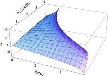
As a rule, the AGW field cannot be approximated without taking the geometric phase into account. Figure 1 illustrates the significance of the geometric phase ${\it\chi}$ , (3.24), in the simple case of a quiescent atmosphere with a constant ${\it\gamma}$ . In figure 1, the dimensionless parameter $h(z)/h(0)$ can be interpreted as the ratio of absolute temperatures at heights $z$ and $z=0$ . The range of sound speeds in the figure, from $c(0)/1.5$ to $2c(0)$ , is close to their range in the real atmosphere; ${\it\chi}$ is shown for propagating waves, for which $m^{2}(z)>0$ and $m^{2}(0)>0$ . For propagation between heights with sufficiently different sound speeds (or, equivalently, air temperatures), the increment of the geometric phase can be as large as $10{\rm\pi}$ (figure 1).

Figure 1.

Geometric phase of AGWs in a quiescent atmosphere. The geometric phase ${\it\chi}(z)$ is shown in radians as a function of dimensionless parameters $h(z)/h(0)=c^{2}(z)/c^{2}(0)$ and $kh(0)$ in an atmosphere with the ratio ${\it\gamma}=1.4$ of specific heats at constant pressure and constant volume; $kg/{\it\omega}^{2}=20$ .

It follows from the dispersion equation (3.5) that propagating AGWs (i.e. waves with real-valued $\boldsymbol{k}$ and $m$ ) exist when either ${{\it\omega}_{d}}^{2}>{\it\Omega}^{2}$ or ${{\it\omega}_{d}}^{2}<N_{0}^{2}$ , where

(3.25a,b ) $$\begin{eqnarray}{\it\Omega}=\frac{c}{2h}=\frac{{\it\gamma}g}{2c},\quad N_{0}^{2}=\frac{g}{h}-\frac{g^{2}}{c^{2}}=\frac{({\it\gamma}-1)g^{2}}{c^{2}}.\end{eqnarray}$$

Since $1<{\it\gamma}<2$ in ideal gases, we have $0<N_{0}<{\it\Omega}$ . Waves with ${\it\omega}_{d}^{2}>{\it\Omega}^{2}$ and ${\it\omega}_{d}^{2}<N_{0}^{2}$ form the acoustic and buoyancy branches of AGWs, respectively. (For a discussion of the acoustic and buoyancy branches, see Hines Reference Hines1960 and Gossard & Hooke Reference Gossard and Hooke1975. In the literature on atmospheric waves, AGWs on the buoyancy and acoustic branches are sometimes loosely referred to as gravity waves and infrasound, respectively.) Under the conditions of figure 1, ${\it\omega}<N_{0}$ , and the results pertain to AGWs on the buoyancy branch.

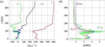
To illustrate the dependence of the geometric phase on the AGW frequency and horizontal wavevector in the real atmosphere, we use the wind velocity and temperature profiles generated by the Whole Atmosphere Model, or WAM (Fuller-Rowell et al. Reference Fuller-Rowell, Akmaev, Wu, Anghel, Maruyama, Anderson, Codrescu, Iredell, Moorthi, Juang, Hou and Millward2008, Reference Fuller-Rowell, Wu, Akmaev, Fang and Araujo-Pradere2010). The WAM description of the atmosphere above southern Iceland, which is shown in figure 2(a), was previously used in modelling long-range propagation of atmospheric waves generated by the 2010 eruption of Eyjafjallajökull volcano (Matoza et al. Reference Matoza, Vergoz, Le Pichon, Ceranna, Green, Evers, Ripepe, Campus, Liszka, Kvaerna, Kjartansson and Hoskuldsson2011; Zabotin et al. Reference Zabotin, Godin, Sava and Zabotina2014). Note that below about 250 km the effective buoyancy frequency $N_{0}$ , which enters the AGW dispersion relation (3.5), varies much more smoothly with height than the buoyancy frequency $N$ (figure 2 b). Unlike $N$ , $N_{0}$ is always positive and smaller than the acoustic cutoff frequency ${\it\Omega}$ ; $N$ and $N_{0}$ are indistinguishable at very high altitudes, where the atmosphere becomes nearly isothermal (figure 2 b).

Figure 2.

Atmospheric stratification. (a) An example of the sound speed $c$ and wind velocity profiles predicted by the Whole Atmosphere Model (Fuller-Rowell et al. Reference Fuller-Rowell, Akmaev, Wu, Anghel, Maruyama, Anderson, Codrescu, Iredell, Moorthi, Juang, Hou and Millward2008, Reference Fuller-Rowell, Wu, Akmaev, Fang and Araujo-Pradere2010; Zabotin et al. Reference Zabotin, Godin, Sava and Zabotina2014);  $u_{x}$ and $u_{y}$ are the zonal (from west to east) and meridional (from south to north) components of the wind velocity. (b) Atmospheric parameters that constrain the frequencies of propagating AGWs. Buoyancy frequency $N$ , the effective buoyancy frequency $N_{0}$ , and the acoustic cutoff frequency ${\it\Omega}$ are defined in the text and are calculated for the sound-speed profile shown in (a) assuming that ${\it\gamma}=1.4$ and $g=9.8~\text{m}~\text{s}^{-2}$ .

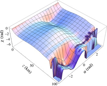
In the real atmosphere, the geometric phase ${\it\chi}$ , (3.13), of AGWs with frequencies ${\it\omega}_{d}<N_{0}$ can be both positive and negative (figure 3). Its sign is mostly opposite that of the eikonal $S$ , (3.23), at heights $0<z<100~\text{km}$ . Variations of the geometric phase with height can exceed $2{\rm\pi}$ and, because of the wind, strongly depend on the direction of the horizontal wavevector $\boldsymbol{k}$ unless the trace velocity $C={\it\omega}/k$ is large compared to the wind speed. (The trace velocity is the reciprocal of the magnitude of the horizontal slowness $\boldsymbol{k}/{\it\omega}$ of the wave and has the meaning of the phase speed of the trace of the wave on the horizontal plane.) More rapid variations of ${\it\chi}$ are associated with stronger winds and larger temperature and wind velocity gradients (figures 2 and 3).

Figure 3.

Geometric phase at various heights and azimuthal directions of propagation for atmospheric waves on the buoyancy branch of the AGWs. Wave frequency $f=2~\text{mHz}$ and horizontal wavevector $\boldsymbol{k}=2{\rm\pi}\,f\,C^{-1}(\cos {\it\alpha},\sin {\it\alpha},0)$ with the trace speed $C=60~\text{m}~\text{s}^{-1}$ . Parameters of the atmosphere are shown in figure 2.

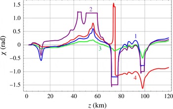
On the acoustic branch of AGWs, the geometric phase ${\it\chi}$ tends to zero in the limit of high frequencies, but remains significant when the wave frequency is of the order of the acoustic cutoff frequency (figure 4). The intervals of heights where waves are evanescent, i.e.  $m^{2}<0$ , contribute to neither ${\it\chi}$ , (3.13), nor the eikonal $S$ , (3.23), and account for the horizontal segments of lines 1 and 2 in figure 4. The geometric phase is sensitive to small variations in wave frequencies and trace speed, especially when a turning point approaches the heights where gradients of air temperature or wind velocity are large (figure 4).

Figure 4.

Geometric phase as a function of height for waves on the acoustic branch of the AGWs in the atmosphere with parameters shown in figure 2. Wave frequencies $f={\it\omega}/2{\rm\pi}$ and trace speeds $C={\it\omega}/k$ are 4.5 mHz and $400~\text{m}~\text{s}^{-1}$ (1); 4.65 mHz and $380~\text{m}~\text{s}^{-1}$ (2); 5 mHz and $400~\text{m}~\text{s}^{-1}$ (3); and 5 mHz and $380~\text{m}~\text{s}^{-1}$ (4). Horizontal wavevector $\boldsymbol{k}=(2{\rm\pi}\,f\,C^{-1},0,0)$ .

3.3. Validity of the WKB solutions when turning points are present

While the WKB solutions diverge at turning points $z=z_{t}$ , where $m(z_{t})=0$ , the solutions remain valid outside a layer $|z-z_{t}|<d_{t}$ , which proves to be narrow compared to the spatial scale $L$ of $c$ , $\boldsymbol{u}$ , and $h$ variations. Consider a turning point $z=z_{t}$ , such that there are no other singular points of the WKB solutions in the vicinity $|z-z_{t}|\ll L$ of $z_{t}$ . To evaluate $d_{t}$ and find the domain of applicability of the first WKB approximation in the vicinity of the isolated turning point, we will follow Brekhovskikh & Godin (Reference Brekhovskikh and Godin1998) and require that the difference between the first and second WKB approximations is small.

In the vicinity $|z-z_{t}|\ll L$ of the isolated turning point, from (3.5) we have

(3.26) $$\begin{eqnarray}m^{2}=\pm {\it\mu}^{2}\cdot ({\it\zeta}-{\it\zeta}_{t})[1+O({\it\zeta}-{\it\zeta}_{t})],\end{eqnarray}$$

where ${\it\zeta}_{t}=z_{t}/L$ and ${\it\mu}^{2}$ is a representative value of $|m^{2}|$ away from the turning point. Equations (3.9), (3.10), and (3.26) give $f_{1}={\it\mu}^{2}O(m^{-1})$ and $f_{2}={\it\mu}^{4}O(m^{-5})$ . The second WKB approximation differs from the first approximation (3.12) by the factor

(3.27) $$\begin{eqnarray}E_{2}({\it\zeta})=L^{-1}\int _{0}^{{\it\zeta}}f_{2}({\it\zeta}_{1})\,\text{d}{\it\zeta}_{1},\end{eqnarray}$$

see (3.3) and (3.6). Here, $f_{2}$ and $E_{2}$ diverge, when ${\it\zeta}\rightarrow {\it\zeta}_{t};~E_{2}=({\it\mu}L)^{-1}O(({\it\zeta}-{\it\zeta}_{t})^{-3/2})$ . For the first WKB approximation to be applicable, it is necessary that $|E_{2}|\ll 1$ and, therefore, $|{\it\zeta}-{\it\zeta}_{t}|\gg ({\it\mu}L)^{-2/3}$ . In terms of dimensional height $z$ , the applicability condition becomes

(3.28) $$\begin{eqnarray}|z-z_{t}|\gg ({\it\mu}^{-2}L)^{1/3},\end{eqnarray}$$

or $d_{t}\sim ({\it\mu}^{-2}L)^{1/3}$ . Thus, the vicinity of the turning point, where the first WKB approximation is invalid, is large compared to the vertical scale ${\it\mu}^{-1}$ of the wavefield variation away from the turning point but is small compared to the scale $L$ of the $c$ , $\boldsymbol{u}$ , and $h$ variations.

Within its domain of applicability, the WKB approximation predicts a large increase of the wave amplitude in the vicinity of the turning point. According to (3.12), (3.15), (3.26), and (3.28), $|{\it\rho}^{-1/2}\tilde{p}|$ and $|{\it\rho}^{-1/2}p|$ in the vicinity of the turning point are amplified by the large factor $O(({\it\mu}L)^{1/3})$ compared to their values away from the turning point on its ‘illuminated’ side, where $m^{2}>0$ and the AGWs are propagating (as opposed to evanescent) waves.

Let us show that the condition (3.28) applies also to higher-order WKB approximations. Assume that

(3.29) $$\begin{eqnarray}f_{n}={\it\mu}^{2n}O(m^{1-3n})\end{eqnarray}$$

for $n=1,2,\dots ,N-1$ . We have already seen that (3.29) holds at $n=0,1$ , and 2. Then, it follows from (3.10) that (3.29) is valid for $n=N$ . Hence, (3.29) is valid for all natural $n$ . According to (3.3) and (3.6), the $n$ th WKB approximation for $\tilde{p}$ differs from the ( $n-1$ )th approximation by the factor $\exp (E_{n}({\it\zeta}))$ , where

(3.30) $$\begin{eqnarray}E_{n}({\it\zeta})=L^{1-n}\int _{0}^{{\it\zeta}}f_{n}({\it\zeta}_{1})\,\text{d}{\it\zeta}_{1}.\end{eqnarray}$$

When ${\it\zeta}\rightarrow {\it\zeta}_{t}$ , it follows from (3.26), (3.29), and (3.30) that $E_{n}=({\it\mu}L)^{1-n}O(({\it\zeta}-{\it\zeta}_{t})^{3(1-n)/2})$ . The necessary condition $|E_{n+1}|\ll 1$ of applicability of the $n$ th approximation with $n>1$ is again given by (3.28). Since (3.28) ensures the smallness of contributions of all higher-order approximations, it is not only a necessary but also a sufficient condition of validity of the first WKB approximation (as an asymptotic solution in the limit $L\rightarrow \infty$ ). A different approach is necessary to obtain rigorous estimates of the deviation of the first WKB approximation from exact solutions at finite $L$ , see Olver (Reference Olver1974), Fedoryuk (Reference Fedoryuk1987), Brekhovskikh & Godin (Reference Brekhovskikh and Godin1998) and references therein.

The condition (3.28) of the WKB approximation validity can be written in a rather intuitive form in terms of the phase integral $S$ , see (3.23). In follows from (3.26) and (3.28) that the WKB approximation is applicable at heights $z$ , where the increment of the phase integral between the current height and the turning point is large compared to unity:

(3.31) $$\begin{eqnarray}|S(z)-S(z_{t})|\gg 1.\end{eqnarray}$$

The WKB applicability conditions (3.28) and (3.31) for AGWs have the same form as in the case of acoustic waves (Brekhovskikh & Godin Reference Brekhovskikh and Godin1998, § 8.1). The condition (3.28) has been derived from the asymptotic series (3.3), (3.6), (3.8)–(3.10) for the Lagrangian pressure perturbation $\tilde{p}$ . As expected, the same result follows from the series (A 1), (A 3)–(A 6) for the vertical displacement $w$ . The necessary reasoning is essentially unchanged and is based on the observation that, as follows from (A 4)–(A 6) and (3.26), the same estimate (3.29) applies to functions $F_{n}$ in (A 3) as to functions $f_{n}$ .

In various ad hoc approximations, which were referred to as ‘WKB approximations’ in Pitteway & Hines (Reference Pitteway and Hines1965), Einaudi & Hines (Reference Einaudi and Hines1970, Reference Einaudi, Hines and Hines1974), Gossard & Hooke (Reference Gossard and Hooke1975), Jones & Georges (Reference Jones and Georges1976) and Fritts & Alexander (Reference Fritts and Alexander2003), the value of $m^{2}$ differs from our (3.5) by the terms ${\it\mu}O(L^{-1})$ , which originate from the terms containing derivatives $\text{d}h/\text{d}z$ , $\text{d}c/\text{d}z$ , and/or $\text{d}{\it\omega}_{d}/\text{d}z$ . In particular, an additional term ${\it\mu}O(L^{-1})$ results from replacement of $g(h^{-1}-gc^{-2})$ with $N^{2}$ , the buoyancy frequency squared, in the last term on the right-hand side of (3.5). The difference between the $m^{2}$ values arising in various ad hoc approximations (Einaudi & Hines Reference Einaudi and Hines1970, Reference Einaudi, Hines and Hines1974) are also ${\it\mu}O(L^{-1})$ , see (3.21) and (3.22). The ad hoc approximations diverge at their respective turning points. An addition ${\it\mu}O(L^{-1})$ to $m^{2}$ shifts the turning point height, i.e. the location of a zero of the function $m^{2}(z)$ , by ${\it\mu}^{-1}O(L^{0})$ , see (3.26). Such a shift is much larger than the vicinity $|z-z_{t}|<d_{t}$ of the actual turning point, where the WKB approximation is not applicable. To rationalize the difference between various ad hoc approximations, Einaudi & Hines (Reference Einaudi and Hines1970, Reference Einaudi, Hines and Hines1974) argued that these approximations differ significantly only when the WKB approximation is not valid. Our analysis of the conditions of the WKB approximation applicability shows that Einaudi & Hines’ argument is fallacious.

3.4. Limiting cases

In the limit $g\rightarrow 0$ , the background fluid density ${\it\rho}$ is no longer related to the background pressure $p_{0}$ by (2.1); the vertical dependencies of $c$ , ${\it\rho}$ , and $\boldsymbol{u}$ can be prescribed independently in a layered fluid with a generic equation of state. In this limit, $p_{0}=\text{const.}$ and $h^{-1}\rightarrow 0$ . For a fluid with a generic equation of state, equation (3.2) for $h$ does not necessarily apply, and the ratio $h(0)/h(z)$ should be understood as ${\it\rho}(z)/{\it\rho}(0)$ , see (3.1). The only type of mechanical wave supported by ideal compressible fluids in the absence of gravity is sound, i.e. acoustic waves. The difference vanishes between the Lagrangian, $\tilde{p}$ , and Eulerian, $p$ , pressure perturbations; wave equations (2.9) and (2.10) reduce to the well-known acoustic wave equation (e.g. Brekhovskikh & Godin Reference Brekhovskikh and Godin1998, § 1.2).

Asymptotic solution of the wave equation simplifies greatly in the acoustic case because parameters of the medium now have only one scale of spatial variations, $L$ , instead of two distinct scales, $L$ and $h$ , in the case of AGWs. In this limit, (3.5), (3.8)–(3.10), which define the WKB series for AGWs, reduce to

(3.32a−c ) $$\begin{eqnarray}m^{2}=\frac{{\it\omega}_{d}^{2}}{c^{2}}-k^{2};\quad f_{0}=\pm m;\quad f_{n}=\frac{1}{2f_{0}}\left(\text{i}f_{n-1}\frac{\text{d}}{\text{d}{\it\zeta}}\ln \frac{f_{n-1}}{{\it\rho}{\it\omega}_{d}^{2}}-\mathop{\sum }_{l=1}^{n-1}f_{l}\,f_{n-l}\right),\quad n\geqslant 1,\end{eqnarray}$$

and agree with the equations (Brekhovskikh & Godin Reference Brekhovskikh and Godin1998, § 8.1) which define the WKB series for acoustic waves and were derived by different means. In particular, in the first WKB approximation (3.12) and (3.13) give ${\it\chi}\equiv 0$ and

(3.33) $$\begin{eqnarray}p(z)=p(0)\sqrt{{\it\rho}{\it\omega}_{d}^{2}m(0)/{\it\rho}(0){\it\omega}_{d}^{2}(0)m}\exp \left(\pm \text{i}\int _{0}^{z}m\,\text{d}z_{1}\right)\end{eqnarray}$$

in agreement with the acoustic result (Brekhovskikh & Godin Reference Brekhovskikh and Godin1998, § 8.2). Obviously, acoustic waves have no Berry phase. This is consistent with the general equation (3.13) for the Berry phase ${\it\chi}$ , where the integrand on the right-hand side vanishes in the acoustic limit. When $\boldsymbol{k}/{\it\omega}$ is independent of frequency, $m/{\it\omega}$ is also independent of frequency according to (3.32). Then, the amplitude and phase of propagating sound waves (3.33) are, respectively, independent of and proportional to ${\it\omega}$ . These properties reflect the well-known fact that sound, unlike AGWs, propagates without dispersion in fluids with gradually varying parameters (e.g. Brekhovskikh Reference Brekhovskikh1960; Brekhovskikh & Godin Reference Brekhovskikh and Godin1998, Reference Brekhovskikh and Godin1999).

In the ad hoc approach (Einaudi & Hines Reference Einaudi and Hines1970, Reference Einaudi, Hines and Hines1974; Gossard & Hooke Reference Gossard and Hooke1975; Jones & Georges Reference Jones and Georges1976; Fritts & Alexander Reference Fritts and Alexander2003) it is implied that the WKB solutions have the form (3.20) with some function $q(z)$ . Equation (3.33) shows that this assumption does not hold even for sound when the fluid is moving or its density varies with $z$ . It follows from (3.21) and (3.22) that the functions $q_{p}(z)/{\it\omega}$ and $q_{w}(z)/{\it\omega}$ retain a dependence on frequency in the acoustic limit. Thus, the unjustified assumption, equation (3.20), about the form of the WKB solutions in the ad hoc approach leads to the unphysical prediction that sound waves are dispersive.

In the opposite limit, where gravity is the dominant restoring force and compressibility of the fluid is negligible, the WKB approach is often applied to study internal gravity waves in the Boussinesq approximation (Garrett Reference Garrett1968; Gill Reference Gill1982, chapter 8; Miropol’sky Reference Miropol’sky2001, chapter 3). For the Boussinesq approximation to be justified, relative changes of the background density ${\it\rho}(z)$ need to be small compared to unity. Therefore, this version of the WKB approximation is not relevant to the atmospheric waves unless the range of heights considered is limited to be within a fraction of the scale height $h$ . A version of the WKB approach, which is suitable for internal gravity waves in incompressible fluids and does not rely on the Boussinesq approximation, is considered in appendix B.

5.1. Plane waves

In the elementary case of a fluid where $c,\boldsymbol{u}$ , and $h$ are independent of height (in particular, in an isothermal ideal gas with constant ${\it\gamma}$ ), governing equations readily reduce to differential equations with constant coefficients (Pierce Reference Pierce1965); linearly independent solutions for ${\it\rho}^{-1/2}\tilde{p},~{\it\rho}^{-1/2}p$ , and ${\it\rho}^{1/2}w$ are just $\exp (\pm \text{i}mz)$ (Lamb Reference Lamb1932; Pierce Reference Pierce1965). Thus, continuous AGWs with a given horizontal wavevector $\boldsymbol{k}$ are a superposition of two plane waves.

In this case, ${\it\chi}\equiv 0$ in (3.12) and (3.13). For $n\geqslant 1$ , $f_{n}\equiv 0$ in (3.9) and (3.10) and $F_{n}\equiv 0$ in (A 5) and (A 6). Then, as expected the WKB solutions (3.12), (3.14), (3.15), and (A 7) reduce to the well-known plane-wave solutions, as do various ad hoc approximations (Einaudi & Hines Reference Einaudi and Hines1970, Reference Einaudi, Hines and Hines1974). A more stringent test of the validity of the approximate solutions is provided by another exact solution (Godin Reference Godin2012a , Reference Godin2014a ), which describes a particular type of AGWs in arbitrarily stratified fluids.

5.2. Incompressible wave motion in compressible fluids

Arbitrarily stratified compressible fluids with uniform background flow support AGWs with the dispersion equation (3.18), in which $\tilde{p}\equiv 0$ ,

(5.1a,b ) $$\begin{eqnarray}p=g{\it\rho}w,\quad w(z)=w(0)\text{e}^{kz}.\end{eqnarray}$$

Fluid motion in these waves is incompressible in the sense that $\boldsymbol{{\rm\nabla}}\boldsymbol{\cdot }\boldsymbol{v}\equiv 0$ in accordance with (2.5). With appropriate boundary conditions, solution (5.1) describes a surface wave which propagates horizontally (Godin Reference Godin2012a , Reference Godin2014a ).

In the WKB approach, we have $m^{2}=-(k-1/2h)^{2}$ from (3.5) and (3.18). With $F_{0}=\text{i}(k-1/2h)$ , (A 5)–(A 6) give $F_{n}\equiv 0$ for all $n\geqslant 1$ . Then, the WKB equations (3.16) and (A 7) become exact and coincide with (5.1).

This should be contrasted with predictions of various ad hoc approximations considered by Einaudi & Hines (Reference Einaudi and Hines1970, Reference Einaudi, Hines and Hines1974) and Jones & Georges (Reference Jones and Georges1976). None of these approximations reproduces the exact solution (5.1).

5.3. The WKB series as an exact analytic solution

When an asymptotic series defined by either (3.7)–(3.10) or (A 3)–(A 6) is convergent, the series gives an exact solution for AGWs in a continuously stratified atmosphere. In particular, this is the case when either series has only a finite number of non-zero terms. Therefore, by establishing conditions when the WKB series terminates, one can generate explicit, analytic solutions of the problem. Here, we consider a simple sufficient condition of the WKB series termination.

Let $f_{2}({\it\zeta})={\it\varepsilon}s({\it\zeta})$ , where ${\it\varepsilon}$ is a small parameter and $s({\it\zeta})$ is an infinitely differentiable function. Then, it follows from (3.10) that $f_{n}({\it\zeta})=O({\it\varepsilon})$ for all $n\geqslant 3$ and all ${\it\zeta}$ such that neither of (3.17), (3.18) and $m=0$ holds. Moreover, if $f_{2}({\it\zeta})\equiv 0$ , then $f_{n}({\it\zeta})\equiv 0$ for all ${\it\zeta}$ and $n\geqslant 3$ . Similarly, from (A 6) it follows that $F_{n}({\it\zeta})\equiv 0$ for all $n\geqslant 3$ in the series (A 3) when $F_{2}({\it\zeta})\equiv 0$ . Thus, the first WKB approximation for the Lagrangian pressure perturbations, (3.12) and (3.13), gives exact solutions of the problem, when $f_{2}({\it\zeta})\equiv 0$ ; the first WKB approximation for the vertical displacement, (A 7), gives exact solutions of the problem, when $F_{2}({\it\zeta})\equiv 0$ .

We have seen in §§ 5.1 and 5.2 that $f_{2}({\it\zeta})\equiv 0$ and $F_{2}({\it\zeta})\equiv 0$ for two known exact solutions. However, these equations can help in generating new exact solutions. Exploring the full set of such solutions is beyond the scope of this paper, and we limit ourselves to just a few examples. Three new exact solutions are derived in appendix C.