1. Introduction
Macroeconomic fluctuations and recessions tend to be devastating for aggregate economic activity but also have a significant impact on the income distribution. In particular for the USA, Bitler and Hoynes (Reference Bitler and Hoynes2015) find that the negative effects of recessions are more pronounced on the lower end of the income distribution. This procyclical relationship was even stronger during the Great Recession, which was triggered by the meltdown of the US financial system and the eventual 2009 Global Financial Crisis (GFC). The financial crisis, in turn, has been attributed to the overheating of financial markets caused by the creation of complex financial instruments with underlying risks that were poorly understood by market participants (Stein, Reference Stein2013).
In this paper, we provide a theoretical explanation for these observations, building on an endogenous credit cycle model (Matsuyama et al. Reference Matsuyama, Sushko and Gardini2016). In that model, agents choose between “good” investment projects, which contribute to capital formation, and “bad” projects, which do not but potentially offer higher returns. Investment in bad projects is financially constrained which leads to endogenous (and potentially irregular) business cycle fluctuations. We extend the model along two important dimensions. First, we introduce financial intermediaries who select between the two types of projects to invest. As we explain in more detail below, this extension captures some important features of the GFC. The second extension introduces heterogeneity across agents. This allows us to disentangle the effects of macroeconomic fluctuations on the income distribution between those due to direct effects on factor returns and those due to changes in occupational choice.
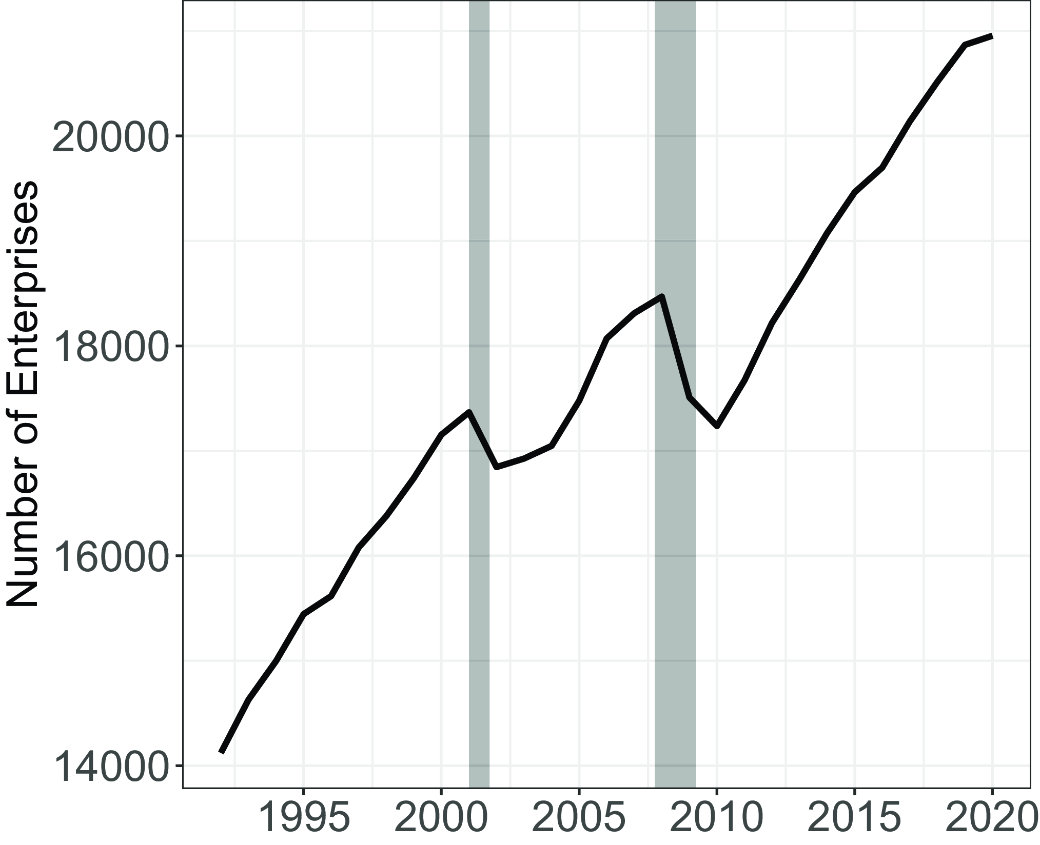
We will show that this heterogeneity is important for understanding the increase in income inequality during the Great Recession identified by Bitler and Hoynes (Reference Bitler and Hoynes2015). Moreover, it allows us to explain the simultaneous decline in the labor and profit income shares, as shown in the left and right panels of Figure 1, respectively. While the labor share shows a secular decline with clear patterns after crises (gray bars), the profit share (based on after-tax profits of non-financial corporations) shows different dynamics. After the dot-com crisis in 2001, it reached an all-time low, gaining pronounced momentum afterwards. Nevertheless, both shares show a procyclical pattern. Moreover, we also observe a decline in the number of firms during recessions, as shown in Figure 2. Our model accounts for these dynamics by explicitly modeling the occupational choice decision.
US labor share (left panel) and US profit share for the non-financial corporate business sector (right panel) in percentage of GDP.
Notes: The left (right) panel shows the US labor (profit) share for the non-financial corporate business sector in percentage of GDP from 1950Q1 to 2023Q2. Corporate profits are after tax excluding IVA (inventory valuation adjustment) and CCAdj (capital consumption adjustment). Gray shaded areas denote the NBER recessionary dates.
Source: Macrobond.

Although there is a lot of research dedicated to understanding the long-term trends of income inequality, the behavior of the latter during cycles has been studied less and primarily within the real business cycle framework.Footnote 1 However, the recent work by Beaudry et al. (Reference Beaudry, Galizia and Portier2020) suggests that business cycles respond to a strong endogenous mechanism driven by financial frictions. Our model provides a theoretical explanation for such a mechanism and studies its implications for income distribution over the cycle.
US enterprises over time.
Notes: This figure shows United States enterprises and firms with 500 or more employees, from 1992 to 2020. Gray shaded areas denote the NBER recessionary dates.
Source: Macrobond.

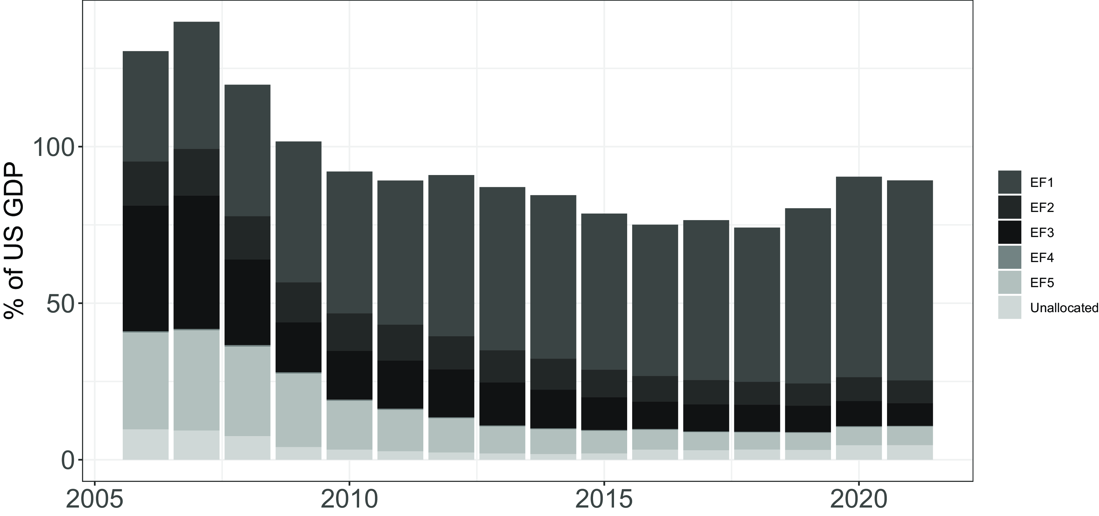
US non-bank financial intermediation by economic function (EF) as percentage of GDP.
Notes: This figure shows the US non-bank financial intermediation by economic function (EF) as percentage of US GDP. Bars from top to bottom: EF1: Management of collective investment vehicles with features that make them susceptible to runs; EF2: Loan provision that is dependent on short-term funding; EF3: Intermediation of market activities that is dependent on short-term funding or on secured funding of client assets; EF4: Facilitation of credit creation; EF5: Securitization-based credit intermediation and funding of financial entities.
Source: Financial Stability Board: Global Monitoring Report.

Our modeling choices are strongly motivated by the banking activities that took place before and during the crisis, which are now documented by numerous sources. For example, the securitization of various banking assets is an activity that has been going on for a long time before the crisis to satisfy the growing demand for investment in safe assets, mainly by institutional investors. Allocation of risk from those who prefer to avoid it to those willing to bear it is one of the main functions of an efficient financial system.
However, it is now well understood that many of the new assets that banks created to achieve this risk reallocation were mispriced. Banks underpriced the risk of the underlying assets on which the performance of the newly created assets depended on (Mizen, Reference Mizen2008). Many complementary explanations have been offered for the mispricing of assets. For example, Gennaioli and Shleifer (Reference Gennaioli and Shleifer2018) emphasize behavioral biases in the formation of investors beliefs, while Richardson and White (Reference Richardson, White, Richardson and White2009) focus on the failure of credit rating agencies to assess the quality of new assets. In Gennaioli et al. (Reference Gennaioli, Shleifer and Vishny2012) mispricing is caused by investors neglecting low-probability risks. Our model is more closely motivated by a fourth explanation that is in general founded on the practices of “shadow banking” and, in particular, the creation of “Special Investment Vehicles” (SIVs).Footnote 2
Prior to the crisis, the banking sector’s liabilities grew dramatically, and as banks sought to maintain high returns on their investments, the average risk of their assets gradually increased. Banks sought to securitize these assets through off-balance sheet SIVs to avoid capital requirements. Figure 3 illustrates this development by showing US non-bank financial intermediation activity by a number of economic functions (EFs) as a percentage of GDP since 2006. Overall, the GFC led to a substantial reduction in non-bank financial intermediation as a result of tighter financial regulation. In particular, complex financial products, such as those associated with securitization-based credit intermediation and financing of financial firms, shown in light gray as EF5, peaked just before the GFC and declined sharply thereafter. On one hand, securitization has fostered the distribution of credit risk; on the other hand, it has disincentivized financial institutions from performing screening and monitoring-related activities (Mian and Sufi, Reference Mian and Sufi2009; Keys et al. Reference Keys, Mukherjee, Seru and Vig2010; Wang and Xia, Reference Wang and Xia2014).
With such exotic products, banks were able to move risky assets off their balance sheets, with the result that their ratings improved and their leverage and investment activities increased (Benmelech and Dlugosz, Reference Benmelech, Dlugosz, Benmelech and Dlugosz2009; Stanton and Wallace, Reference Stanton and Wallace2010). However, according to the “too big to fail” view, banks have also been willing to implicitly provide liquidity guarantees to SIVs and thus retain risk because they could count on a government bailout if things went badly (Acharya and Richardson, Reference Acharya, Richardson, Acharya and Richardson2009). In our model, as the return on bank capital falls, banks shift their investments to bad projects. On the one hand, this allows banks to earn a higher return on their investments, but on the other hand, it diverts credit away from good projects. Thus, they engage in counterproductive activities by not contributing to physical capital formation. For evidence that some banks have knowingly engaged in such activities, see, for example, Griffin (Reference Griffin2021).
Our setup is based on an infinite horizon, discrete time, two-period, overlapping generations model in the spirit of Matsuyama et al. (Reference Matsuyama, Sushko and Gardini2016). Each period a new generation of young agents is born who do not consume but earn wages by finding employment in the final goods sector. At birth, each agent’s productivity is randomly determined. When old, agents can either deposit their wages in the banking system, earning interest income and income from an alternative activity such as self-employment. Alternatively, they can become entrepreneurs by combining their wage income with borrowed funds from the banking system to produce physical capital. Final goods are produced using a Cobb-Douglas technology that combines labor and physical capital. The choice depends on their level of productivity, with more productive agents finding it optimal to become entrepreneurs. Financial intermediation—though enhancing the productivity of firms—is costly which is captured by a constant unit cost of new loans to entrepreneurs for good projects.Footnote 3 Banks have access to an alternative technology (bad projects) that yields a positive temporary return without contributing to the formation of physical capital and thus without generating pecuniary externalities for the next generation. This technology is meant to capture the creation and distribution of the complex financial products mentioned above.Footnote 4
We begin the analysis of our model with the case where bad projects are not available and show that the model is similar to the neoclassical growth model. We obtain a unique steady state that depends negatively on the cost of financial intermediation. Next, we allow banks to invest in bad projects, which are initially assumed to be unconstrained. For economies with relatively efficient banking systems, in the absence of bad projects, the high capital-labor ratio and the corresponding low marginal productivity of capital would have pushed the interest rate below the return on bad projects. Therefore, when bad projects are available, banks reduce the funds lent to entrepreneurs until the lending rate equals the return on bad projects. There is also a unique steady state in this specification, but with a lower capital-labor ratio. Here we deviate from Matsuyama et al. (Reference Matsuyama, Sushko and Gardini2016), as not only the intensive margin (loan size) but also the extensive margin (number of entrepreneurs) adjust to changes in the rate of return. In a final step, we introduce a constraint that captures economies of scale in the production of bad projects. The rationale is that there is a certain threshold of economic development that an economy must reach before its financial system becomes sufficiently advanced to be able to produce complex financial products. As Acharya and Schnabl (Reference Acharya and Schnabl2009) document, the banks involved in the creation of new assets were among the largest financial institutions and located in economies with high per capita GDP. Strong empirical support for the existence of such thresholds is also provided in de la Torre et al. (Reference de la Torre, Feyen and Ize2013). In particular, they observe that “financial services that are strongly inhibited by collective frictions should develop only after a critical mass of participation has been reached that is sufficient to trigger positive externalities needed to sustain their development” (p. 519). With the introduction of the above constraint in our model, the resulting phase map of the capital-labor ratio becomes more complex. Now, the model generates interesting dynamics ranging from unique steady states to regular cycles of varying periodicity to chaotic attractors.Footnote 5
The results of our model resemble empirical evidence on the dynamics of income inequality over the business cycle. Despite the Cobb-Douglas production technology, we observe fluctuations in workers’ income shares. The reason for this is that the financial sector invests in bad—unproductive—investment projects, which transforms the aggregate production function. Similarly, the derivation of aggregate income must take into account the income generated by the production of bad projects. In the fully specified model, recessions are associated with a decline in both the share of profits and the share of labor income explained by the decline in the number of firms. These results are consistent with the stylized facts presented above and with the findings on income inequality in Bitler and Hoynes (Reference Bitler and Hoynes2015). The reason that inequality increases is because there are fewer firms during recessions losing the least productive ones, thus increasing the average profitability. The change in the extensive margin (number of entrepreneurs) means that although profits decline during recessions, they are distributed among a fewer number of entrepreneurs. With respect to the banking sector, for tractability, we assumed that banks earn zero profits. As a result, our model predicts that the group that benefits most from recessions are depositors. However, when we subtract from the income going to depositors the income generated by bad projects, which most likely earned by banks, we find that the share of total income going to depositors has declined. Thus, our model provides a novel theoretical explanation for the impact of business cycles on the distribution of income in an economy with complex financial markets.
The remainder of the paper is organized as follows. In Section 2, we present the model in its general form, derive the equations that govern its dynamics and present analytic results on the shape of the dynamic map and on fixed-point properties. In Section 3, we further specify the functional forms, analyze the evolution of the capital/labor ratio, and prove analytically the existence of cycles for the case when investment in bad projects is constrained. Using a numerical analysis based on parameter values consistent with stylized facts, we further demonstrate how variations in the cost of financial intermediation and the efficiency of financial innovation influence its dynamic behavior. While highlighting the wide variety of possible cyclical dynamics, involving fixed points, cycles of low periodicity, and chaotic attractors, a quite robust pattern of boom and bust cycles emerges. In Section 4, we build on these patterns and examine the impact of cycles on income inequality. We show that the results are robust to (a) a broad choice of parameterizations of the model and (b) the exact characteristics of the dynamic paths. Finally, Section 5 concludes the paper.
Related literature: Central to our model is the link between macroeconomic fluctuations, financial frictions, and financial intermediaries. Following the seminal work of Bernanke et al. (Reference Bernanke, Gertler, Gilchrist, Bernanke, Gertler and Gilchrist1999), a large literature has emerged studying related issues. However, the central framework is mainly based on the real business cycle paradigm, which views cycles as generated by exogenous shocks.Footnote 6 The majority of such model yield a unique steady state. A notable exception is Benhabib et al. (Reference Benhabib, Wang and Dong2018) where the introduction of adverse selection in credit markets generates multiple steady states. In the rest of the review, we limit our attention to those studies, like ours, in which cycles arise endogenously.
The most closely related paper is Matsuyama (Reference Matsuyama2013). Agents have the choice of investing either in good projects that indirectly enhance the future productivity of the economy or in bad projects that are financially constrained. During booms agents net worth is sufficiently high to allow them to invest in bad projects which are more profitable at the detriment of future growth. In contrast, during slumps, agents’ low net worth does not allow agents to invest in bad projects. By investing in good projects they provide the fuel for the next cycle. In our paper, financial intermediaries have the choice of allocating their funds between good projects (offering loans to financially constrained entrepreneurs) and bad projects. We also account for heterogeneity among agents, which allows us to characterize the dynamics of income distributions throughout economic cycles. Other theoretical works, extending the Matsuyama (Reference Matsuyama2013) model, include Matsuyama et al. (Reference Matsuyama, Sushko and Gardini2016) that studies in more detail the stability properties of a slight simpler model and Kubin and Zörner (Reference Kubin and Zörner2021) that augments the model by introducing human capital.
In addition to the endogeneity of fluctuations, financial frictions due to agency problems are common to all of the above models. Thus, another strand of the literature, to which the present paper belongs, deals with frictions affecting the intermediation process. For example Chousakos et al. (Reference Chousakos, Gorton and Ordoñez2023) and Gorton and Ordoñez (Reference Gorton and Ordoñez2020) examine the impact of information generated about firms’ quality of collateral and productivities on the evolution of output which, in turn, affects the incentives to acquire such information. This process generates complex dynamics that lead to cycles. In Myerson (Reference Myerson2012), there is financial moral hazard, which is rooted in the ability of large financial institutions to abuse their power in deciding how to invest large amounts of other people’s wealth. In particular, the success of projects depends on whether bankers make an effort to monitor them. Optimal solutions require that bankers be compensated based on long-term performance. However, this implies that there are periods when trustworthy managers are scarce and aggregate investment declines. In Dong and Xu (Reference Dong and Xu2020), there is misallocation of resources due to the ability of banks to divert funds borrowed in the interbank market. To mitigate the moral hazard problem, lending banks impose credit constraints on borrowing banks. In a dynamic setting, the interaction of credit restrictions and the allocation of capital among projects with different productivity can lead to shifts between a well-functioning interbank market equilibrium and another in which it collapses. Finally, Sunaga (Reference Sunaga2017) shows that economic cycles are generated as the intensity of entrepreneurial innovation interacts with the endogenous ability of banks to screen good ideas.
In another strand of the literature, there are frictions on the demand side for funds. In Azariadis and Smith (Reference Azariadis and Smith1998), for example, cycles arise as the economy moves between a Walrasian regime with no binding constraints and one with credit rationing introduced to solve self-selection problems due to adverse selection. In contrast, a moral hazard type of friction is introduced by Suarez and Sussman (Reference Suarez and Sussman1997). In this model, lenders must incentivize firms to exert effort and increase the probability of project success. During booms, prices, and thus liquidity, fall, increasing the demand for external funds, which results in excessive risk-taking, low returns, and eventually a recession. Conversely, when quantities decrease, prices rise, reducing the demand for liquidity and the level of risk-taking. In Kiyotaki and Moore (Reference Kiyotaki and Moore1997), verifiability concerns imply that lenders are unable to force borrowers to repay their loans and thus only provide loans that are secured. In such an economy, assets play a dual role as (a) productive capital and (b) collateral. The dynamic interaction between asset prices and credit limits leads to amplified and persistent fluctuations in aggregate output. Lastly, Gu et al. (Reference Gu, Mattesini, Monnet and Wright2013) examine the role of limited commitment, where borrowers are unable to commit not to divert the funds lent to them to alternative uses. The endogeneity of debt limits imposed by lenders to reduce diversion incentives interacts with investor beliefs, leading to cycles.Footnote 7
Complementing this strand of the literature, another approach builds on the classical Goodwin framework by introducing financial frictions on the supply side. In his seminal contribution, Goodwin (Reference Goodwin and Goodwin1967) analyzed growth cycles through out-of-equilibrium dynamics, emphasizing the interaction between employment and income distribution. This framework has since been extended to include credit constraints and financial market imperfections to better capture macro-financial linkages. For example, Sordi and Vercelli (Reference Sordi and Vercelli2014) allow for disequilibrium in the goods market and incorporate borrowing constraints, showing that financial frictions can suppress the labor share over the cycle. Our findings are consistent with this result, though the mechanism differs: in our case, the decline in the labor share is driven by excessive investment in bad projects during downturns. While Giraud and Grasselli (Reference Giraud and Grasselli2021) explore how rising household indebtedness shapes long-run inequality, our analysis focuses on cyclical fluctuations in inequality.
A crucial feature of our model in generating cycles is the presence of economies of scale in the production of bad projects. As we elaborate below, this mechanism can stem from complementarities arising through diversification benefits. Several studies have explored the relationship between different types of complementarities and business cycles. For instance, Eeckhout and Lindenlaub (Reference Eeckhout and Lindenlaub2019) analyze labor market complementarities driven by search externalities. Similarly, search externalities play a key role in Fernández-Villaverde et al. (Reference Fernández-Villaverde, Mandelman, Yu and Zanetti2021, Reference Fernández-Villaverde, Mandelman, Yu and Zanetti2024), where firms exert effort to establish trading relationships. Finally, Schaal and Taschereau-Dumouchel (Reference Schaal and Taschereau-Dumouchel2015) adopt a dynamic games approach to examine coordination failures resulting from demand complementarities and increasing returns to scale. While these studies emphasize complementarities in labor markets or demand-side interactions, our model introduces a novel perspective by focusing on externalities within the financial sector. This distinction highlights how financial-market dynamics can independently generate cyclical fluctuations through economies of scale in bad project production.
2. The model
Time is discrete and extends infinitely
 $(t=0,1,2\ldots )$
. At each date a generation of unit mass is born and lives for two periods. Agents of each generation are distinguished by their type
 $z$
. The distribution of types
 $ G(z)$
is continuous, time invariant with support on
 $[$
 $\underline{z }\,,\bar {z }]$
and corresponding density function
 $g(z)$
. Agents consume only when they are old. Young agents, born at
 $t$
, are endowed with
 $z$
units of (effective) labor that they supply inelastically for the production of the final good. We normalize the aggregate supply of labor to
 $1$
, thus
 $\int _{\underline {z}}^{\bar {z}}zg(z)dz=1$
.
There is one final good that can either be consumed or invested. The final good can be produced by a constant returns-to-scale technology (CRS),
 $ f(k_{t})$
, where
 $k_{t}$
denotes the capital/labor ratio at
 $t$
. For all
 $t$
,
 $f^{^{\prime }}(k_{t})\gt 0\gt f^{\prime \prime }(k_{t})$
,
 $f(0)=0$
and the Inada condition
 $ f^{\prime }(k)\rightarrow \infty$
as
 $k\rightarrow 0$
holds. Physical capital fully depreciates in one period and both factor markets are competitive. Then, the reward to physical capital is equal to
 $\rho _{t}=$
 $ f^{^{\prime }}(k_{t})$
, which is decreasing in
 $k_{t}$
and reward to labor is equal to
 $W(k_{t})=f(k_{t})-k_{t}f^{^{\prime }}(k_{t})\equiv W(k_{t})\gt 0$
, which is increasing in
 $k_{t}$
. Thus a type
 $z$
agent’s wage income is equal to
 $zW(k_{t})$
.
Old agents have two options. The first option is to deposit their wages in the perfectly competitive banking system and obtain interest income and income
 $y$
from self-employment (measured in units of the final good).Footnote
8
The second option is to borrow from the banking system and use the loan together with their endowment to produce physical capital which is then invested in the CRS technology to produce the final good. Physical capital is produced by using the final good as input, whereby each unit of final good yields
 $R$
units of physical capital.Footnote
9
The amount of the final good that agents can borrow from the banking system also depends on their type. In particular, a type
 $z$
agent will be able to borrow a maximum amount of
 $(m-1)zW(k_{t})$
units of the final good from the bank at the gross interest rate
 $r_{t+1}^{b}$
and therefore invest a total amount of
 $mzW(k_{t})$
.
 $m$
in our model is equivalent to the equity multiplier in the Holmström and Tirole (Reference Holmström and Tirole1997) variable investment model.Footnote
10
The same type
 $z$
agent will earn income
 $f^{^{\prime }}(k_{t+1})R(m)zmW(k_{t})$
, repay
 $ r_{t+1}^{b}(m-1)zW(k_{t})$
to the bank, and consume the difference. Agents of the same type who choose to deposit their labor income in the banking system will consume
 $r_{t+1}^{d}zW(k_{t})+y$
. Thus, as long as,
 \begin{equation} f^{^{\prime }}(k_{t+1})R(m)zmW(k_{t})-r_{t+1}^{b}\left ( m-1\right ) zW(k_{t})\gt r_{t+1}^{d}zW(k_{t})+y, \end{equation}
agents of type
 $z$
will invest in the physical capital technology. An agent will be indifferent, if (1) holds with equality. By setting (1) as an equality we can solve for a threshold value of endowments,
 $z^{\ast }$
, such that all agents with endowments above this value become entrepreneurs.
One key benefit of financial intermediation is that it enhances firm productivity through the services it provides.Footnote
11
We capture this effect through the function
 $R=R(m)$
, where
 $R^{\prime }\gt 0$
.Footnote
12
Additionally, financial intermediaries improve welfare through a second channel. In the absence of a banking system, agents have only two options: they can invest their endowments to become entrepreneurs or earn income through self-employment
 $y$
. Clearly, agents with low endowments would prefer the second option. Financial intermediation allows them to earn some income on their endowments through deposits and some additional income
 $y$
from self-employment. Banks have two options about how to invest their deposits. They can either offer loans to agents who invest in the physical capital technology or they can invest in a one-period “bad” technology that yields
 $B$
units of the final good at
 $\left ( t+1\right )$
for each unit of the final good invested at
 $t$
. Investment in these projects is unproductive as it does not contribute to the stock of physical capital.Footnote
13
Banking services are costly. The cost per unit of loan is equal to
 $\gamma$
units of the final good. Clearly if
 $r_{t+1}^{b}\lt B(1+\gamma )$
banks will choose to invest in the bad technology. Let
 $V_{t+1}$
denote the total investment in the bad technology. We assume that investment in bad projects is constrained by the size of the economy. As we mentioned above there is empirical evidence that suggests that the extent of the market due to economies of scale and network effects is a very important contributing factor to the ability of the banking system to introduce financial innovation (de la Torre et al. Reference de la Torre, Feyen and Ize2013). In particular we assume that the maximum amount that can be invested,
 $\hat {V}\left ( k_{t}\right )$
, with
 $\hat {V}^{\prime }\left ( k_{t}\right ) \gt 0$
, depends on the level of the capital/labor ratio which is a good proxy for the size of the economy and, hence, the size of the banking system.Footnote
14
The generation of cyclical fluctuations in our model depends on the first derivative,
 $\hat {V}^{\prime }\left ( k_{t}\right ) \gt 0$
. With economies of scale arising from either/both the demand side (e.g., the demand of derivatives depends on the size of the banking sector) or/and the supply side (economies of scale in financial innovation) bad projects become available relatively fast and, as we describe below, cycles become possible.
Market clearing in financial markets requires that
 \begin{equation} \int \limits _{z_{t+1}^{\ast }}^{\bar {z}}(1+\gamma )\left ( m-1\right ) zW(k_{t})g(z)dz+V_{t+1}=\int \limits _{\underline {z}}^{z_{t+1}^{\ast }}zW(k_{t})g(z)dz. \end{equation}
The left-hand side equals the total funds available for loans (that also includes the cost of these loans) and the total funds invested in bad projects. The right-hand side equals aggregate deposits.
Each entrepreneur invests her endowment
 $zW(k_{t})$
plus her funds borrowed from banks,
 $(m-1)zW(k_{t})$
, to produce
 $R(m)$
units of physical capital. Thus, the evolution of the capital/labor ratio is given by
 \begin{equation} k_{t+1}=R(m)mW(k_{t})\int \limits _{z_{t+1}^{\ast }}^{\bar {z}}zg(z)dz. \end{equation}
The exact form of equation (3) depends on whether there is investment in bad projects and, if so, whether that investment is constrained.
2.1 Bad projects are not available
Consider the case where the banking system does not invest in the bad technology,
 $V_{t+1}=0$
. Given that the left-hand side of (1) is increasing in
 $z$
, agents with low initial endowments prefer to become depositors and those with high initial endowments prefer to become entrepreneurs. Market clearing requires that the aggregate amount of loans is equal to aggregate deposits,
 \begin{equation*} \int \limits _{z_{t+1}^{\ast }}^{\bar {z}}(1+\gamma )\left ( m-1\right ) W(k_{t})zg(z)dz=\int \limits _{\underline {z}}^{z_{t+1}^{\ast }}W(k_{t})zg(z)dz. \end{equation*}
On the left hand side, we have the allocation of funds between loans and expenditure to cover the cost of banking services. On the right-hand side, we have aggregate deposits. The above condition implies that
 $z_{t+1}^{\ast }=z^{\ast }$
for every
 $t$
and is the solution of
 \begin{equation} 1=\left ( m+\gamma m-\gamma \right ) \int \limits _{z^{\ast }}^{\bar {z} }zg(z)dz. \end{equation}
The banking system’s zero-profit condition when
 $V_{t+1}=0$
is given by
 \begin{equation*} r_{t+1}^{b}\int \limits _{z^{\ast }}^{\bar {z}}\left ( m-1\right ) W(k_{t})zg(z)dz=r_{t+1}^{d}\int \limits _{\underline {z}}^{z^{\ast }}W(k_{t})zg(z)dz. \end{equation*}
Using the market clearing condition, the zero-profit condition implies that
 \begin{equation} r_{t+1}^{b}=r_{t+1}^{d}\left ( 1+\gamma \right ) \text{ for every }t\text{ such that }V_{t+1}=0. \end{equation}
Each entrepreneur invests her endowment
 $zW(k_{t})$
plus her funds borrowed from banks,
 $(m-1)zW(k_{t})$
, to produce
 $R(m)$
units of physical capital. Using (4) we can write (3) as
 \begin{equation} k_{t+1}\equiv F\left ( k_{t}\right ) =\frac {R(m)m}{m+\gamma m-\gamma }W(k_{t}). \end{equation}
Dynamic stability requires that
 $F^{\prime }\left ( k_{t}\right ) \gt 0$
,
 $ F^{\prime \prime }\left ( k_{t}\right ) \lt 0$
and
 $F^{\prime }(k)\rightarrow \infty$
as
 $k\rightarrow 0$
, (see Figure 4).Footnote
15
Lastly, substituting (4) and (5) in (1) determines implicitly the equilibrium interest rates,
 $r_{t+1}^{d}$
and
 $r_{t+1}^{b}$
, such that an agent of type
 $z^{\ast }$
is indifferent between investing and saving (depositing).
Financial repression.

To obtain the steady state, we set
 $k_{t+1}=k_{t}=k^{\ast }$
in (6). Proposition1 describes comparative statics at the steady state:
Proposition 1.
Suppose that bad projects are not available, i.e.,
 $V_{t+1}=0$
, and
 $\gamma$
is small, then
 $\frac {dk^{\ast }}{dm}\lt 0,\frac {dk^{\ast }}{d\gamma } \lt 0,\frac {dk^{\ast }}{dy}=0,$
and
 $\frac {dz^{\ast }}{dm}\gt 0,\frac {dz^{\ast }}{d\gamma } \gt 0,\frac {dz^{\ast }}{dy}=0.$
Proof. The proposition directly follows from totally differentiating (4) and (6) and from the dynamic stability condition.
The qualification on
 $\gamma$
is necessary only for the first result, as
 $m$
influences the steady-state capital-labor ratio through two distinct channels. First, by relaxing the financing constraint, an increase in
 $m$
promotes growth by enhancing project productivity. Second, a higher
 $m$
leads to a greater volume of lending, which, given the costs associated with loans, negatively impacts capital accumulation. Notably,
 $z^{\ast }$
is independent of
 $y$
. The economic intuition is that an increase in
 $y$
requires a lower interest rate to ensure the marginal old agent remains indifferent. Furthermore,
 $k^{\ast }$
decreases with
 $\gamma$
(see Figure 4). In economies with high intermediation costs, financial repression leads to a lower steady-state capital-labor ratio, as a significant share of potentially productive capital is absorbed by the operational and administrative expenses of granting new loans.
2.2 Investment in bad projects: the unconstrained case
The derivations in the previous section apply as long as
 $ r_{t+1}^{b}\geqslant B\left ( 1+\gamma \right )$
. However, if
 $ r_{t+1}^{b}\lt B\left ( 1+\gamma \right )$
the banking system will invest some of the deposits in the bad technology,
 $\ V_{t+1}\gt 0$
. For the moment we concentrate on the case where the investment in bad projects is not constrained, which is
 $\hat {V}(k_{t})\approx \infty$
.
The market clearing condition now is given by (2). For the banking system to be indifferent between lending and investing in the bad technology, we must have
 $r_{t+1}^{b}=B(1+\gamma )$
. The banking system’s zero-profit condition is given by
 $r_{t+1}^{b}\int \nolimits _{z_{t+1}^{\ast }}^{\bar {z}}\left ( m-1\right ) W(k_{t})zg(z)dz+BV_{t+1}^{\ast }=r_{t+1}^{d}\int \nolimits _{\underline {z}}^{z_{t+1}^{\ast }}W(k_{t})zg(z)dz$
, which implies (using equation (2)) that
 \begin{equation} r_{t+1}^{b}=B(1+\gamma )\gt r_{t+1}^{d}=B\quad \text{ for every }t\text{ such that }V_{t+1}\gt 0. \end{equation}
The stock of physical capital at
 $k_{t+1}$
is given by (3). Given that in equilibrium an agent of type
 $z_{t+1}^{\ast }$
must be indifferent between investing and saving (depositing) (1) implies that the following equality must hold:
 \begin{equation} z_{t+1}^{\ast }W(k_{t})(f^{^{\prime }}(k_{t+1})R(m)m-B(m+\gamma m-\gamma )) =y. \end{equation}
Then, for given
 $W(k_{t})$
, we can solve (3) and (8) together for
 $k_{t+1}$
and
 $z_{t+1}^{\ast }$
and then by substituting the solution for
 $ z_{t+1}^{\ast }$
in (2) we can solve for
 $V_{t+1}^{\ast }$
.
As noted in the introduction, a key distinction between our paper and Matsuyama et al. (Reference Matsuyama, Sushko and Gardini2016) is that we move beyond the representative agent framework by introducing heterogeneity in initial endowments. In Matsuyama et al. (Reference Matsuyama, Sushko and Gardini2016), when investment in bad projects is unconstrained, the capital-to-labor ratio remains independent of its previous-period value. This is because it is solely determined by the condition that marginal productivity equals the constant return on bad projects. In contrast, our model determines equilibrium returns endogenously. Specifically, when the loan market clears, the marginal agent remains indifferent between becoming an entrepreneur and depositing their endowment in the bank and becoming self-employed.
Let
 \begin{equation} k_{t+1}\equiv H(k_{t})=R(m)mW(k_{t})\int \limits _{z_{t+1}^{\ast }}^{\bar {z} }zg(z)dz \end{equation}
denote the evolution of the capital/labor ratio when investment in bad projects is unconstrained.
Proposition 2.
Suppose that investment in bad projects is unconstrained. Then,
 $H^{\prime }(k_{t})\gt 0$
and
 $\frac {dz_{t+1}^{\ast }}{dk_{t}}\gtrless 0$
.
Proof. See Appendix A.
When investment in bad projects is not constrained, the evolution of the capital/labor ratio follows an upward path, once we allow for heterogeneous agents. There are two effects responsible for that result. In contrast to Matsuyama et al. (Reference Matsuyama, Sushko and Gardini2016), the last period’s capital stock matters when investment in bad projects is not constrained. The reason is that agents with higher endowments benefit more from being entrepreneurs. To restore indifference the return of good projects has to decline which means the capital/labor ratio must go up. There is also a second adjustment that takes place through a change in the cut-off endowment level that separates the two types of old agents. More specifically, the number of entrepreneurs decreases, i.e.,
 $z_{t+1}^{\ast }$
increases, if
 $\frac {d^{2}f\left ( k_{t+1}\right ) }{dk_{t}^{2}}$
is sufficiently low.
Phase map of the capital/labor ratio.
Notes: This figure shows the phase map of the capital/labor ratio. The parameter values used are
 $R=2.5$
,
 $A=2.5$
,
 $m=1.5$
,
 $ \gamma =0.03$
,
 $y=1$
,
 $B=1.25$
,
 $k^{FG}=6$
, and
 $ \delta =-1.25$
.
 $F(k_{t})$
,
 $G(k_{t})$
, and
 $H(k_{t})$
refer to the respective branch of the map where
 $k^{FH}$
,
 $k^{FG}$
, and
 $k^{FH}$
denote the respective thresholds.

This result is driven by a direct and an indirect effect (as can be seen from (8)): An increase in
 $k_{t}$
, that increases
 $W(k_{t})$
and thus the incentive to become an entrepreneur, reduces—ceteris paribus, i.e., keeping
 $k_{t+1}$
constant—the cut-off (and the number of entrepreneurs would increase). However, there is an indirect effect due to the increase in next period’s capital/labor ratio (
 $H^{\prime }(k_{t})\gt 0$
).
 $ k_{t+1}$
increases,
 $f^{^{\prime }}(k_{t+1})$
declines and the incentive to become an entrepreneur is reduced (the cut-off increases). Only if the indirect effect dominates the direct effect, the overall result will be an increase in the cut-off and a reduced number of entrepreneurs (see Appendix A for the exact condition). These adjustments not only result in a richer dynamic behavior of our model relative to Matsuyama et al. (Reference Matsuyama, Sushko and Gardini2016) but also have important implications for the variations of income inequality in both the long run and within the business cycle (see Section 4).
In Figure 5 below, we can compare—for a fixed
 $\gamma$
—the evolution of the capital/labor ratio
 $k_{t+1}$
when bad projects are not available (the higher dark blue line depicting
 $k_{t+1}=F(k_{t})$
) with the case when bad projects are available and investment in bad projects is not constrained,
 $ k_{t+1}=H(k_{t})$
, in light blue. For future reference, we denote the point of intersection
 $k^{FH}$
. For
 $k_{t}=k^{FH}$
we have
 $r_{t+1}^{b}=B\left ( 1+\gamma \right )$
so that the banking system is indifferent between offering loans to entrepreneurs and investing in bad projects. Banks begin to invest in bad projects when
 $H(k_{t})\lt F(k_{t})$
, meaning that the capital/labor ratio
 $k_{t+1}$
is lower than it would be if such investments were not available.
Importantly,
 $H(k_{t})$
is upward sloping, which is in significant contrast to Matsuyama et al. (Reference Matsuyama, Sushko and Gardini2016), where the corresponding branch of the function is flat. In this model there is a representative agent, who adjusts her capital/labor ratio. In our model with heterogeneous agents, physical capital adjusts along two margins. Borrowing terminology from the international trade literature, over time the capital/labor ratio not only adjusts along the intensive margin as entrepreneurs of the same type adjusts their output levels (as in Matsuyama et al. Reference Matsuyama, Sushko and Gardini2016), but also along the extensive margin as the proportion of entrepreneurs changes.
As soon as
 $k_{t}$
grows to the level where the return to good projects is equal to the return of the bad projects all additional savings are invested in bad projects so that the two returns stay equal. Thus, in Matsuyama et al. (Reference Matsuyama, Sushko and Gardini2016), the function corresponding to
 $H(k_{t})$
is flat. In our model, agents are heterogeneous and therefore adjustments can happen on both margins. Our simulations shown below confirm that even with investments in bad projects, there is still a positive relationship between
 $k_{t}$
and
 $k_{t+1}$
(on
 $ H(k_{t})$
). They illustrate the case in which as
 $k_{t}$
and
 $ k_{t+1}$
increase the threshold
 $z_{t+1}^{\ast }$
increases, that is, the mass of entrepreneurs decreases.
Note that this is also different from the evolution of capital/labor along
 $ F(k_{t})$
. In the absence of bad projects as
 $k_{t}$
increases the return to capital, and hence the two interest rates, decline. In fact the decline in the interest rate just compensates for the increase in the capital/labor ratio so that the marginal agent is still indifferent between becoming an entrepreneur or depositing her wages in the bank and becoming self-employed, so there is no adjustment on the extensive margin and
 $z_{t+1}^{\ast }$
remains constant. However, on
 $H(k_{t})$
the interest rate on deposits is equal to the return of the bad projects (adjusted for the cost of loans) and does not drop as some of the extra capital is invested in bad projects. There is also an adjustment on the extensive margin.
Finally, comparing the evolution of the capital-to-labor ratio in the case where bad projects are unavailable, as given by equation (6), with the case where investment in bad projects is unconstrained, implicitly represented by equation (9), we find that the latter is indirectly influenced by changes in the level of self-employment
 $y$
and the return on bad projects,
 $B$
. This influence occurs through their effect on the threshold level
 $z_{t+1}^{\ast }$
(see equation (8)), whereas these variables do not affect equation (6). This observation is also important for understanding the main methodological contribution of our paper relative to Matsuyama et al. (Reference Matsuyama, Sushko and Gardini2016).
To obtain the steady state we set
 $k_{t+1}=k_{t}=k^{\ast }$
and
 $ z_{t+1}^{\ast }=z^{\ast }$
in (8) and (9).
Proposition 3.
Suppose that investment in bad projects is unconstrained,
 $V_{t+1}\gt 0$
, and
 $\gamma$
is small, then
 $\frac {dk^{\ast }}{dm} \gt 0,\frac {dk^{\ast }}{ d\gamma }\lt 0,\frac {dk^{\ast }}{dy}\lt 0,\frac {dk^{\ast }}{dB}\lt 0,$
and
 $\frac {dz^{\ast }}{dm}\gtrless 0,\frac { dz^{\ast }}{d\gamma }\gtrless 0,\frac {dz^{\ast }}{dy}\gtrless 0,\frac { dz^{\ast }}{dB}\gtrless 0.$
Proof. See Appendix A.
Any increase in
 $y$
or
 $B$
by encouraging investment in bad projects has a negative effect on
 $k^{\ast }$
. This is because an increase in
 $y$
makes it more attractive to agents depositing their endowments at the bank, thus increasing the supply of funds and depressing the interest rate. This favors investment in bad projects which can also be the result of a direct increase in the return of bad projects. Therefore, either of the above two changes shifts
 $H(k_{t})$
downwards moving the intersection with the
 $45^{\circ }$
-line to the left and below the original intersection and as a result
 $k^{\ast }$
will decrease (see Figure 5). When bad projects are unavailable, we previously established that an increase in
 $m$
positively affects
 $k^{\ast }$
as long as
 $\gamma$
remains small. Now, an additional effect emerges: banks have less incentive to invest in bad projects, as the rising return on capital leads to higher interest rates. As a result, the positive impact of
 $m$
on
 $k^{\ast }$
is even stronger. The comparative statics of
 $z^{\ast }$
depend on both direct and indirect effects, making the overall impact indeterminate unless further restrictions are imposed on the functional forms of production functions and the distribution of endowments.
2.3 Investment in bad projects: the constrained case
Finally, consider the case when the investment in bad projects is constrained. The following two conditions must hold: (a)
 $r_{t+1}^{b}\lt B\left ( 1+\gamma \right )$
when there is no investment in bad projects, and (b)
 $V_{t}\gt \hat {V} \left ( k_{t}\right )$
, where
 $V_{t}$
denotes the level of investment in bad projects that would have been obtained had such investment been unconstrained. Exactly because this investment is constrained the borrowing rate and the return to bad projects are not equalized. Now market clearing implies that
 $\int \nolimits _{z_{t+1}^{\ast }}^{\bar {z}}(1+\gamma )\left ( m-1\right ) W(k_{t})zg(z)dz+\hat {V}\left ( k_{t}\right ) =\int \nolimits _{\underline {z}}^{z_{t+1}^{\ast }}W(k_{t})zg(z)dz$
, which can be written as:
 \begin{equation} 1=\left ( m+\gamma m-\gamma \right ) \int \limits _{\underline {z}}^{z_{t+1}^{\ast }}zg(z)dz+\frac {\hat {V}\left ( k_{t}\right ) }{W\left (k_{t}\right ) }. \end{equation}
Let
 \begin{equation} k_{t+1}\equiv G(k_{t})=R(m)mW(k_{t})\int \limits _{z_{t+1}^{\ast }}^{\bar {z} }zg(z)dz \end{equation}
denote the evolution of the capital/labor ratio when the investment in bad projects is constrained.
Proposition 4.
Suppose that the investment in bad projects is constrained. If
 $\hat {V} ^{\prime }\left ( k_{t}\right )$
is sufficiently high then
 $G^{\prime }(k)\lt 0$
and
 $\frac {dz_{t+1}^{\ast }}{dk_{t}}\gt 0$
.
Proof. See Appendix A.
 $\hat {V}\left ( k_{t}\right )$
indicates the availability of bad projects. As we argued above, strong economies of scale implies that after the economy has reached a threshold level financial innovation and, hence, the availability of bad projects, accelerates. For sufficiently high values of
 $ \hat {V}^{\prime }\left ( k_{t}\right )$
we have
 $G^{\prime }(k_{t})\lt 0$
which is necessary for the existence of cycles. To obtain the steady state, we set
 $k_{t+1}=k_{t}=k^{\ast }$
and
 $ z_{t+1}^{\ast }=z^{\ast }$
in (10) and (11).
Proposition 5.
Suppose that investment in bad projects is constrained,
 $V_{t}=\hat {V}\left ( k_{t}\right )$
, then
 $\frac {dk^{\ast }}{dm}\gtrless 0,\frac {dk^{\ast }}{ d\gamma }\lt 0$
and
 $\frac {dz^{\ast }}{dm}\gtrless 0,\frac {dz^{\ast }}{ d\gamma }\gtrless 0.$
Proof. See Appendix A.
An increase in the cost of banking
 $\gamma$
depresses the capital/labor by reducing the availability of loans. Other things equal, this has a positive effect on the number of producers of good projects even if each one is offered a smaller loan. However, as bad projects offer a better return now this increases the incentives to deposit endowments at the bank having the opposite effect on the threshold. Once more, without imposing further restrictions on the functional forms of the distribution and production functions the effect of changes in financial constraints on
 $z^{\ast }$
remains ambiguous.
3. Dynamics and cycles
3.1 The dynamic map and its functional specification
In Figure 5, we present the complete phase map of the capital/labor ratio. The dark blue line, defined in (6) as
 $F(k_{t})$
, corresponds to that part of the map of the capital/labor ratio when there is no investment in bad projects. Banks would like to invest in bad projects when the light blue line falls below the dark blue line, i.e., for
 $k_{t}\gt k^{FH}$
.Footnote
16
Beyond that point investment in bad projects offers a higher return to the banks than lending to entrepreneurs. However, as the level of economic development does not support financial innovation, they cannot do so because such investment is not available. As soon as the dark blue line intersects the red line, defined in (11) as
 $G(k_{t})$
, banks begin to invest in bad projects which become available as a result of financial innovation. Here we assume that the availability increases sufficiently rapid to generate a negative slope of
 $G(k_{t})$
. We denote the intersection of the two segments,
 $F(k_{t})=G(k_{t})$
, as
 $k^{FG}$
. As long as the red line is above the light blue line, which is defined by (9) as
 $H(k_{t})$
, the investment in bad projects is constrained. As soon as
 $H(k_{t})$
intersects
 $ G(k_{t})$
, investment in bad projects is unconstrained and the evolution of the capital/labor ratio is captured by the light blue line. We denote the intersection of the last two segments of the map at
 $G(k_{t})=H(k_{t})$
as
 $ k^{GH}$
.
Then, we can define the whole dynamic map as:
 \begin{equation} k_{t+1}=\left \{ \begin{array}{l@{\quad}ll} F(k_{t}) & \text{if} & k_{t}\leq k^{FG} \\ G(k_{t}) & \text{if} & k^{FG}\lt k_{t}\lt k^{GH} \\ H(k_{t}) & \text{if} & k^{GH}\leq k_{t} \end{array} \right . . \end{equation}
The phase map of the evolution of the capital/labor ratio, and, hence, its dynamic path, is very similar to the one obtained by Matsuyama et al. (Reference Matsuyama, Sushko and Gardini2016). However, there is an added complexity due to the heterogeneity of agents according to their initial endowments. In this model, physical capital adjusts along two margins: (a) the intensive margin as entrepreneurs of the same type adjusts their output levels, and (b) the extensive margin as the proportion of entrepreneurs changes.
One of the implications of this added complexity is that the part of the map that corresponds to the case when investment in bad projects is unconstrained has always a positive slope while the corresponding part in Matsuyama et al. (Reference Matsuyama, Sushko and Gardini2016) is flat. The reason is that in the in this model as long as the capital/labor ratio is sufficiently high, so that the interest on borrowing (which in turn depends on the marginal product of physical capital) is less than the return on bad projects, the following period’s capital/labor ratio will drop to ensure that the two returns are equal. However, in our paper there is a second margin of adjustment. The interest rate that banks charge to entrepreneurs will still be equal to the return of the bad projects but not the marginal productivity of capital which also depends on the fraction of entrepreneurs (which changes as well, see Proposition2).
This added complexity limits our ability to study the dynamics of the full model analytically, and therefore, we explore its properties by mostly relying on numerical analysis. In order to do so, we have to specify functional forms for the dynamic map. In particular, we use a Cobb-Douglas production function and we linearize the
 $G(k_{t})$
function. The specifications are summarized in the following Proposition:
Proposition 6.
Suppose that the production function is symmetric Cobb-Douglas,
 $f(k)=Ak^{ \frac {1}{2}}$
, and the distribution of endowments is uniform,
 $g(z)\sim U[0,2]$
.Footnote
17
(a) If
 $k_{t}\leq k^{FG}$
then
 \begin{equation*} k_{t+1}=F(k_{t})=\frac {1}{2}\frac {R(m)mA}{m+\gamma m-\gamma }k_{t}^{\frac {1}{2} } \end{equation*}
with the corresponding steady-state solution given by:
 \begin{equation*} k^{\ast }=\left ( \frac {\frac {1}{2}R(m)A}{1+\gamma (1-\frac {1}{m})}\right ) ^{ \frac {1}{2}}. \end{equation*}
(b) For
 $k^{FG}\lt k_{t}\lt k^{GH}$
we impose the following linear functional form on
 $G(k_{t})$
:
 \begin{equation*} k_{t+1}=G(k_{t})=\delta \left ( k_{t}-k^{FG}\right ) +F\left ( k^{FG}\right ) =\delta \left ( k_{t}-k^{FG}\right ) +\frac {R(m)mA}{m+\gamma m-\gamma }\frac { \sqrt {k^{FG}}}{2}. \end{equation*}
This specification ensures that
 $G(k_{t})$
passes through the point
 $\left ( k^{FG},F\left ( k^{FG}\right ) \right )$
and
 $\delta$
approximates its slope. The corresponding steady-state solution is given by:
 \begin{equation*} k^{\ast }=\frac {1}{1-\delta }\left ( -\delta k^{FG}+\frac {R(m)A}{1+\gamma (1- \frac {1}{m})}\frac {\sqrt {k^{FG}}}{2}\right ) . \end{equation*}
(c) If
 $k^{GH}\leq k_{t}$
then the solution for
 $H(k_{t})$
is implicitly defined by the fourth degree polynomial:
 \begin{equation*} \Phi _{4}x^{4}+\Phi _{3}x^{3}+\Phi _{2}x^{2}+\Phi _{1}x+\Phi _{0}=0, \end{equation*}
where
 $x=\sqrt {k_{t+1}}$
,
 $\Phi _{4}\equiv B^{2}(m+\gamma m-\gamma )^{2}k_{t}^{\frac {1}{2}}$
,
 $\Phi _{3}\equiv -AR(m)mB(m+\gamma m-\gamma )k_{t}^{ \frac {1}{2}}$
,
 $\Phi _{2}\equiv \frac {\left ( AR(m)m\right ) ^{2}}{4}k_{t}^{\frac { 1}{2}}-B^{2}(m+\gamma m-\gamma )^{2}\frac {AR(m)m}{2}k_{t}+\frac {R(m)my^{2}}{2A}$
,
 $ \Phi _{1}\equiv \frac {\left ( AR(m)m\right ) ^{2}}{2}B\left ( m+\gamma m-\gamma \right ) k_{t}$
and
 $\Phi _{0}\equiv -\frac {\left ( AR(m)m\right ) ^{3}}{8}k_{t}$
. The corresponding steady-state solution is determined by the following third degree polynomial:
 \begin{equation*} \Psi _{3}\left ( x^{\ast }\right ) ^{3}+\Psi _{2}\left ( x^{\ast }\right ) ^{2}+\Psi _{1}x^{\ast }+\Psi _{0}=0,\end{equation*}
where
 $\Psi _{3}\equiv B^{2}(m+\gamma m-\gamma )^{2}$
,
 $\Psi _{2}\equiv -mR(m)AB(m+\gamma m-\gamma )\left ( 1+\frac {1}{2}(m+\gamma m-\gamma )B\right )$
,
 $\Psi _{1}\equiv m^{2}R(m)^{2}A^{2}\left ( \frac {1}{4}+\frac {1}{2}(m+\gamma m-\gamma )B\right )$
and
 $\Psi _{0}\equiv -R(m)m\left ( \frac {1}{8} m^{2}R(m)^{2}A^{3}-\frac {1}{2A}y^{2}\right )$
.
Proof. See Appendix B for the complete solution of the model.
Before proceeding to numerical simulations, we provide complete analytical results for the case when the investment in bad projects is always constrained, that is
 $F(k^{FG})\lt k^{GH}$
. The inequality implies that the dynamics in the interval
 $[0,k^{GH}]$
involve only the first two branches
 $F$
and
 $G$
. Despite these restrictions, we show that the dynamics of the model are still very complex involving a rich menu of oscillations from periodic cycles to chaotic attractors.
Proposition 7.
Let the map (
12
) with the specifications given in Proposition
6
be restricted only to the
 $F(k_{t})$
and
 $G(k_{t})$
branches in the interval
 $ [0,k^{GH}].$
For
 $k^{\ast }=k^{FG}$
let
 $G^{\prime }(k^{\ast })=G^{\prime }(k^{FG})=\delta .$
Assuming
 $\delta \lt 0$
, and
 $F(k^{FG})\lt k^{GH}$
, then the following results apply.
Property 1
When
 $F(k^{FG})\leq k^{FG},$
the fixed point solution belongs only to the first branch,
 $k^{\ast }\leq k^{FG}$
, and is attracting in the interval
 $[0,k^{GH}]$
.
Property 2
When
 $F(k^{FG})\gt k^{FG},$
the fixed point does not belong to the first branch, and the interval
 $J=[G(F(k^{FG})),F(k^{FG})]$
is absorbing for
 $k_{t}\in \lbrack 0,k^{GH}]$
.Footnote
18
Property 3
When
 $F(k^{FG})\gt k^{FG}$
the transition of the fixed point solution from the first branch to the second one, occurring when the intersection point of the
 $F$
and
 $G$
branches is an equilibrium solution for both branches, i.e.,
 $k^{\ast }=k^{FG}$
, is a border collision bifurcation.
Footnote
19
After the bifurcation, for
 $-1\lt \delta \lt 0$
the fixed point solution
 $k^{\ast }\gt k^{FG}$
is stable; for
 $\delta \lt -1$
the fixed point is unstable.
For
 $-2\lt \delta \lt -1,$
an attracting 2-cycle exists;
for
 $-4\lt \delta \lt -3,$
an attracting 3-cycle exists;
for
 $-8\lt \delta \lt -7,$
an attracting 4-cycle exists;
for
 $-16\lt \delta \lt -15,$
an attracting 5-cycle exists;
any other value of
 $\delta \lt -1$
(i.e., values of
 $\delta$
between the existence of attracting cycles and
 $\delta \lt -16$
) lead to attracting chaotic intervals (a unique interval, or
 $2n$
or
 $n$
cyclical intervals, for
 $ n=1,2,3,4$
).
Proof. See Appendix B.
Remark 1. As we noted above, a necessary condition for the existence of cycles is that
 $\delta \lt -1$
. That is, after the economy reaches the threshold, bad projects become quickly available.
Remark 2. The border collision of Property 3 occurs at
 $A^{BC} = 2\frac {m+\gamma m-\gamma }{mR(m)}k^{FG}$
.
It is not surprising that the numerical analysis below confirms that, broadly, the dynamic behavior of our model is similar to the one in Matsuyama et al. (Reference Matsuyama, Sushko and Gardini2016) although the introduction of agent heterogeneity has added some, from an economic point of view, interesting complexities. In particular, the inclusion of both margins in our model offers a much richer picture of the behavior of income inequality over the business cycle. The model is consistent with a great variety of equilibrium dynamic paths that depend on the values of particular parameters. There are cases where such paths converge to a unique steady state. But more often we find that the paths converge to cycles that are either regular or irregular and of various degrees of periodicity including chaotic dynamics.
However, in the following numerical explorations, we focus on low-period cycles, as these allow for a more transparent economic interpretation in terms of boom-and-bust dynamics. This choice supports our goal of linking endogenous fluctuations to economically meaningful mechanisms and revealing structural dynamics, rather than emphasizing complex or chaotic behavior per se.Footnote 20
3.2 Numerical solution
Our model is intentionally stylized and not suited for exact calibration; instead, we explore its behavior across a wide range of economically plausible parameterizations, aiming to remain as consistent as possible with key stylized facts. The debt-to-total-assets ratio for most non-financial firms is between
 $0$
and
 $1/2$
, corresponding to
 $m$
values of
 $1$
and
 $2$
. Thus, we set
 $m=1.5$
. The value of
 $R$
is equal to the inverse price of capital formation, given that we use the final good as the numeraire and assume full capital depreciation at the end of each period. According to the Penn World Tables (Feenstra et al. Reference Feenstra, Inklaar and Timmer2015, PWT Version 10.01), the average price level of capital formation relative to the price level of U.S. GDP during the period 1950–2019 is approximately
 $0.4$
, implying
 $R=2.5$
. The cost of loans,
 $\gamma$
, in a competitive banking system can be approximated by the net interest rate margin, i.e., the difference between bank lending and deposit rates. Over the last 10 years, the margin for U.S. banks has been around 3 percentage points.Footnote
21
The value of
 $y$
is set to 1 because, for this value, our simulations align with empirical evidence. Specifically, Hamilton (Reference Hamilton2000) finds that, over a 10-year period, average earnings from self-employment were 35% lower than wages. On average, across all our simulations, the ratio of depositors’ income (which includes both savings income and self-employment income) to wages closely matches this value.
In our bifurcation simulations below, we focus on three core parameters:
 $A$
,
 $\delta$
, and
 $\gamma$
, which we vary over a broad range. Parameters
 $\delta$
and
 $\gamma$
directly influence the bank’s project choices, thereby shaping the mechanism that generates cycles in our model. Changes in
 $\delta$
affect the availability of bad projects, while variations in
 $\gamma$
reflect the cost of financing good projects. We find that increases in the loan cost
 $\gamma$
produce qualitatively similar results to increases in the return of bad projects,
 $B$
, and thus we do not vary the latter. Similarly, variations in
 $\gamma$
have effects opposite to those of changes in the benefits of intermediation, represented by
 $m$
. We prefer to present results in terms of
 $\gamma$
rather than
 $m$
, as the latter depends on the specification of
 $R(m)$
. While our qualitative results remain robust to alternative specifications, the quantitative results are sensitive. Therefore, we select fixed values for
 $m$
and
 $R$
that align with their long-run averages. Finally, variations in
 $A$
capture changes in economic productivity. By setting
 $k_{FG} = 6$
(implying
 $A^{BC} = 1.97$
) and varying
 $A$
between
 $2$
and
 $3.5$
we illustrate the analytic results beyond the border collision (see Property 3 in Proposition7 and Remark 2). The full set of parameter values for our benchmark calibration is as follows:
 \begin{equation*} R = 2.5, \quad A = 2.5, \quad m = 1.5, \quad \gamma = 0.03, \quad \delta = -1.25, \quad y = 1, \quad B = 1.25, \quad k^{FG} = 6. \end{equation*}
3.2.1 Numerical analysis: variations in
 $\delta$

In this section, we fix all other parameters at their benchmark values mentioned above and focus on
 $\delta$
. Recall that
 $\delta$
is the slope of the
 $G(k_{t})$
branch, when investment in bad projects is constrained. More rapid generation of bad projects is reflected in a steeper
 $G(k_{t})$
branch, thus in a lower
 $\delta$
value. We let
 $\delta$
vary over a wider range to produce the bifurcation diagram shown in Figure 6. The diagram shows the values of the capital/labor ratio approach asymptotically fixed points and periodic cycles as we vary
 $\delta$
. A small interval with chaotic attractors is also visible. We provide a detailed description of the economic mechanism behind these dynamics.
Bifurcation on
 $\delta$
.
Notes: This figure shows the bifurcation diagram of
 $k$
on parameter
 $\delta$
. The parameter values are:
 $-3\leq \delta \leq 0$
,
 $A=2.5$
,
 $\gamma =0.03$
,
 $R=2.5$
,
 $m=1.5$
,
 $y=1$
,
 $B=1.25$
,
 $k^{FG}=6$
.

Given that
 $\delta$
takes negative values it is more convenient to describe what happens as its values decrease (increase in absolute terms). For very high values of
 $\delta$
(close to zero) we have convergence to a unique steady state. Availability of bad projects is relatively low. In terms of Figure 5, as
 $\delta$
decreases the red line gets steeper by rotating clockwise. As the economy grows it begins to oscillate eventually converging to a unique steady state (on the red line).
For slightly lower values of
 $\delta$
the fixed point loses stability and we obtain stable period-
 $2$
cycles as shown in Figure 7. In this case, the economy rotates between a high capital/labor ratio state with no investment in bad projects, which we denote by A, and a low capital/labor ratio state with constrained investment in bad projects, denoted by B. We refer to this period-
 $2$
cycle as Type 1. When in some period
 $\left ( t-1\right )$
the capital/labor ratio and, hence, wages are high, at period
 $t$
there will be a lot of funds available and banks will invest some of them in bad projects (but not as much as they would if the availability of bad projects was unconstrained). The reason is that if all funds were lent to entrepreneurs, the marginal productivity of capital, and hence the equilibrium borrowing interest rate would drop well below the return to bad projects. However, in the new equilibrium the interest rate will still be below the return of bad projects given that the level of financial innovation is not extensive enough to create a quantity of bad projects consistent with the equalization of the two rates. As some funds are invested in bad projects the new equilibrium capital/labor in period
 $t$
, and hence the wage rate, is below that of period
 $\left ( t-1\right )$
. Then, at
 $\left ( t+1\right )$
the new level of deposits would be too low to support financial innovation and all funds will now be lent to entrepreneurs. The new higher capital/labor ratio marks the beginning of a new cycle.
Type 1 period-2 cycle.
Notes: This figure shows the phase map and the corresponding period-2 cycle, which we refer to as Type 1. The parameter values used are
 $R=2.5$
,
 $A=2.5$
,
 $m=1.5$
,
 $ \gamma =0.03$
,
 $y=1$
,
 $B=1.25$
,
 $k^{FG}=6$
and
 $ \delta =-1.25$
.

Period-4 mixed cycle.
Notes: This figure shows the phase map and the corresponding period-4 mixed cycle. The parameter values used are
 $R=2.5$
,
 $A=2.5$
,
 $m=1.5$
,
 $ \gamma =0.03$
,
 $y=1$
,
 $B=1.25$
,
 $k^{FG}=6$
and
 $ \delta =-2$
.

For still lower values of
 $\delta$
we enter a small region where high periodicity cycles appear including chaotic attractors. But eventually the economy settles into a period-
 $4$
cycle (see Figure 8). Now in one of the low states the investment in bad projects is constrained while in the other low state this investment is unconstrained. We refer to this cycle as a Mixed Period-
 $4$
Cycle. Suppose that at
 $\left ( t-1\right )$
the economy has reached the high capital/labor ratio state. Next period the level of deposits will allow some investment in bad projects but the level of financial innovation constrains that investment. Because at
 $t$
the investment in bad projects was constrained the capital/labor ratio and, thus, wages did not drop as much as they would have done had the investment in bad projects being unconstrained. Thus, at
 $\left ( t+1\right )$
the economy moves to a very high capital/labor ratio. This is because (a) the previous period the investment in bad projects was constrained thus allowing for more lending to entrepreneurs, and (b) this period there is no investment in bad projects. Next, the good performance of the economy in period
 $\left ( t+1\right )$
means that at
 $\left ( t+2\right )$
there are plenty of deposits, intensive financial innovation and unconstrained investment in bad projects which, in turn, implies that the economy has moved to the very low capital/labor ratio state. Next, period there will not be any investment in bad projects and the economy enters a new cycle.
Lastly, for very low values of
 $\delta$
, financial innovation is very efficient and the economy follows a new period-
 $2$
cycle shown in Figure 9. We will refer to this cycle as Type 2 Period-
 $2$
Cycle. In terms of Figure 5 the red line is much steeper. Now investment in bad projects is unconstrained given that the interest rate banks receive on their loans, after adjusting for the costs of creating new loans, is equal to the return on bad projects.
Type 2 period-2 cycle.
Notes: This figure shows the phase map and the corresponding period-2 cycle, which we refer to as Type 2. The parameter values used are
 $R=2.5$
,
 $A=2.5$
,
 $m=1.5$
,
 $ \gamma =0.03$
,
 $y=1$
,
 $B=1.25$
,
 $k^{FG}=6$
and
 $ \delta =-3$
.

Bifurcation on
 $A$
.
Notes: This figure shows the bifurcation diagram of
 $k$
on parameter
 $A$
. The parameter values are:
 $1.5\leq A\leq 3.5$
,
 $ \gamma =0.03$
,
 $R=2.5$
,
 $m=1.5$
,
 $ \delta =-1.25$
,
 $y=1$
,
 $B=1.25$
,
 $k^{FG}=6$
. Vertical lines denote from left to right,
 $2.5$
,
 $2.66$
, and
 $2.8$
, respectively.

3.2.2 Numerical analysis: variations in
$A$

Figure 10 shows the bifurcation diagram for
 $A$
, where there are five distinct regions.Footnote
22
For very low values of
 $A$
, we observe a unique steady state. Since the productivity of good projects is low, the capital-labor ratio and wages are also low. Consequently, the banking sector remains too small to support financial innovation, and no investment occurs in bad projects. As
 $A$
increases, the economy enters a region of Type 1 Period-
 $2$
Cycles (A and B). Here, the economy alternates between periods where the capital-labor ratio is high with no investment in bad projects and periods where the capital-labor ratio is low, leading banks to invest in bad projects, albeit in a constrained manner.
Further increases in
 $A$
move the economy into a region of Type 2 Period-
 $2$
Cycles (C and D). In this regime, the productivity of good projects is sufficiently high so that, in periods with no investment in bad projects, wages and savings rise. As a result, in the following period, the banking sector expands enough to support financial innovation at a level that allows unconstrained investment in bad projects. Even higher values of
 $A$
introduce a new type of cycle where investment in bad projects occurs in every period. However, in one state, investment remains constrained, while in the other state, it is unconstrained. We refer to this type of cycle, illustrated in Figure 11, as the Type 3 Period-
 $2$
Cycle (E and F). In this case, even when investment in bad projects is unconstrained, the economy performs well enough to sustain financial innovation in the subsequent period, albeit at a lower level.
Finally, for very high values of
 $A$
, the economy converges once again to a unique steady state, where investment in bad projects is always unconstrained. Despite the large allocation of funds to bad projects, the capital-labor ratio remains sufficiently high. The high productivity of good projects supports the level of financial innovation necessary to set the equilibrium interest rate equal to the return on bad projects.
Type 3 period-2 cycle.
Notes: This figure shows the phase map and the corresponding period-2 cycle, which we refer to as Type 3. The parameter values are:
 $R=2.5$
,
 $ \gamma =0.03$
,
 $A=2.8$
,
 $m=1.5$
,
 $ \delta =-1.25$
,
 $y=1$
,
 $B=1.25$
, and
 $k^{FG}=6$
.

3.2.3 Numerical analysis: variations in
$ \gamma$

Finally, we turn to the cost of banking and vary
 $\gamma$
over a wide range (while keeping the other parameters at their benchmark). Figure 12 shows the bifurcation diagram for
 $\gamma$
.
For very high values of the cost of lending, the economy always converges to a unique steady state where there is no financial innovation and no investment in bad projects. The banking system becomes highly inefficient, allocating too many resources to its operations rather than offering funds to entrepreneurs. As the cost of lending declines, the economy eventually enters a region characterized by Type 1 Period-
 $2$
Cycles. However, despite the decline in lending costs, too many resources are still absorbed by the cost of providing loans to entrepreneurs. As a result, aggregate economic activity can only support a moderate level of financial innovation, and investment in bad projects remains constrained.
Bifurcation on
 $\gamma$
.
Notes: This figure shows the bifurcation diagram of
 $k$
on parameter
 $\gamma$
. The parameter values are:
 $0\leq \gamma \leq 1$
,
 $R=2.5$
,
 $A=2.5$
,
 $m=1.5$
,
 $ \delta =-1.25$
,
 $y=1$
,
 $B=1.25$
, and
 $k^{FG}=6$
.

4. Inequality and cycles
Above we have identified a great variety of equilibrium dynamic paths that arise as the parameters of the model vary. Some of these paths are simple, converging to a unique steady state, other paths are converging to regular finite-order cycles, and still other more complex paths are characterized by chaotic long-run cyclical dynamics. In this section, we study the behavior of income inequality along these cycles. In particular, we analyze how the steady-state dynamics of the economy change as we vary (a) the availability of bad projects, captured by
 $\delta$
, and (b) the cost of lending, captured by
 $\gamma$
. The purpose of this exercise is to try to understand how income inequality, and, in particular, income shares of workers, entrepreneurs, and depositors vary along economic cycles.
Below, we focus the discussion on a Type 1 Period-2 cycle; however, our numerical analysis of income distribution covers dynamics along all types of Period-2 cycles. Along a Type 1 cycle the economy keeps rotating between a state where aggregate deposits are low and there is no investment in bad projects (point B in Figure 7) to a state where aggregate deposits are high and banks now invest some of their deposits into bad projects but this investment is still constrained (point A in Figure 7). The equilibrium dynamics of the economy along this path are as follows. Suppose at time
 $ \left ( t-1\right )$
, the capital/labor ratio and wages are low. Then, at
 $t$
bad projects will not be available for investment and all deposits will be lent to entrepreneurs. In this state
 $z^{\ast }$
is relatively low and thus the proportion of old agents who become entrepreneurs will be relatively high. The high capital/labor ratio at time
 $t$
implies that the marginal productivity of capital and the interest rates in the same period are low. As the interest rates are low, banks would have liked to invest some of their deposits in bad projects, however, the latter are not available. Because of the high capital/labor ratio wages at
 $t$
are also high. At
 $ \left ( t+1\right )$
there are more funds available for investment but now bad projects become available. As a result the funds available to entrepreneurs are low, increasing the threshold
 $z^{\ast }$
, and hence, the corresponding capital/labor ratio drops. The increase in the marginal productivity of capital implies that interest rates rise but are still below the return of bad projects. This is because the availability of bad projects is constrained. Wages now drop and the cycle is completed.
Next, consider the income of each type of agent along the cycle. At any given date
 $t$
there are two generations of equal size alive. We need to consider the incomes of three types of agents:
-
1. The average income of young agents (half of the population) born at
$t$
is equal to
$W(k_{t})$
(remember endowments are uniformly distributed on
$ [0,2]$
and the mass of young agents is equal to
$1$
, thus
$g(z)=\frac {1}{2}$
. -
2. A proportion
$\frac {2-z_{t}^{\ast }}{2}$
of old agents borrow from the banks and become entrepreneurs. As a group, they earnDividing by
\begin{eqnarray*} &&\int \limits _{z_{t}^{\ast }}^{2}\left ( f^{^{\prime }}(k_{t})R(m)mzW(k_{t-1})-r_{t}^{b}(m-1)W(k_{t-1})\right ) zg\left ( z\right ) dz= \\ &=&\frac {4-\left ( z_{t}^{\ast }\right ) ^{2}}{4}\left ( f^{^{\prime }}(k_{t})R(m)m-r_{t}^{b}(m-1)\right ) W(k_{t-1}). \end{eqnarray*}
$\frac {2-z_{t}^{\ast }}{2}$
results in the average entrepreneurial income:Note that
\begin{equation*} \frac {2+z_{t}^{\ast }}{2}\left ( f^{^{\prime }}(k_{t})R(m)m-r_{t}^{b}(m-1)\right ) W(k_{t-1}). \end{equation*}
$\frac {2+z_{t}^{\ast }}{2}$
is the average endowment of one entrepreneur.
-
3. A proportion
$\frac {z_{t}^{\ast }}{2}$
of old agents deposit their wages at the bank and become self-employed. As a group, they earn income equal toDividing by
\begin{equation*} \int \nolimits _{0}^{z_{t}^{\ast }}\left ( r_{t}^{d}zW(k_{t-1})+y\right ) g\left ( z\right ) dz=\frac {\left ( z_{t}^{\ast }\right ) ^{2}}{4} r_{t}^{d}W(k_{t-1})+\frac {z_{t}^{\ast }}{2}y. \end{equation*}
$\frac {z_{t}^{\ast }}{2}$
results in the average depositor income:
\begin{equation*} \frac {z_{t}^{\ast }}{2}r_{t}^{d}W(k_{t-1})+y. \end{equation*}


The interest rate income is equal to
 $\frac {z_{t}^{\ast }}{ 2}r_{t}^{d}W(k_{t-1})$
and
 $y$
is the income from self-employment. Note that,
 $\frac {z_{t}^{\ast }}{2}$
is also the average endowment of the depositors. Clearly the income of workers (young agents) is procyclical given that wages are increasing with the capital/labor ratio. Entrepreneurial income of a given type is countercyclical because of the marginal productivity of capital and the fact that along the cycle
 $k_{t}$
and
 $W(k_{t-1})$
move in the same direction. Part of the decline in the marginal productivity of capital during booms is compensated by the decline in the borrowing interest rate. Nevertheless, total entrepreneurial income and, thus final good output, increases because the mass of entrepreneurs has increased. Financial income (income from deposits) is also countercyclical because of the fall in the interest rates when the capital/labor ratio rises. In our model banks make zero profits so all returns from bad projects accrue to depositors. With this in mind we calculate separately that part of financial income generated by bad projects (more likely to be earned by financial institutions). In our numerical examples below, where we subtract that income from the overall income earned from deposits we find that the remained income (most likely received by depositors) is procyclical.Footnote
23
The increase in the threshold that separates entrepreneurs from depositors during recessions exacerbates the increase in inequality between entrepreneurs and the other two groups. There are fewer entrepreneurs each earning more. Lastly, given that all incomes are linearly increasing with
 $z$
, any increase in the marginal payoff of a group also increases the income dispersion within that group.
4.1 Numerical analysis
We present numerical results for each of the three Period-2 Cycles defined above. What we find is that the qualitative effects of business cycles on income inequality are robust not only to changes in the parameter values but also as we move from one type of cycle to another. The following parameter values are the same in all three numerical examples:
 \begin{equation*} \gamma =0.03,R=2.5,m=1.5,y=1,B=1.25\text{ and }k^{FG}=6. \end{equation*}
The Type 1 period-2 Cycle (A and B) is presented for
 $A=2.5$
and
 $\delta =-1.25$
(as used for Figure 7); the Type 2 period-2 Cycle (C and D) is presented for
 $A=2.5$
and
 $\delta =-3$
(as used for Figure 9); the Type 3 period-2 Cycle (E and F) is presented for
 $A=2.8$
and
 $\delta =-1.25$
(as used for Figure 11). Table 1 shows, for each type of cycle, the proportions of each type of agent, the corresponding aggregate income for each group of agents, and the average income within each group (for workers who have a unit measure, aggregate and average income are the same). In all three types of cycles, the proportion of entrepreneurs increases as the economy moves from the low states (points B, D, and F) to the high states (A, B, and C) because investment in bad projects decreases, and thus banks lend more funds to entrepreneurs. Those who gain in high states are workers, as the higher capital/labor ratio implies that the marginal productivity of labor increases. Entrepreneur income is countercyclical because of the decline in the marginal productivity of capital during booms. However, as a group, they earn more because their numbers significantly increase during booms. Our numerical results also show that the income of depositors, after subtracting the part earned from bad projects, is procyclical.
Impact of cycles on income distribution dynamics

Notes: The parameter values are as follows. Type 1:
 $A=2.5$
and
 $\delta =-1.25$
; Type 2:
 $A=2.5$
and
 $\delta =-3$
; Type 3:
 $A=2.8$
and
 $\delta =-1.25$
; the other parameters are at their baseline values (
 $\gamma =0.03,R=2.5,m=1.5,y=1,B=1.25$
and
 $k^{FG}=6$
).
We are also interested in understanding the impact of cycles on the relative shares of entrepreneurs and workers, as well as on inequalities within groups. Table 2 below shows the income shares of each group of agents along the two phases of each of the three types of cycle, using the same parameter values as those in Table 1. We find that entrepreneurial shares are procyclical, while average entrepreneurial income is countercyclical. This is because the higher proportion of entrepreneurs during periods of expansion more than compensates for the decline in productivity. While we have set the share factor in the Cobb-Douglas function equal to
 $0.5$
, the share of wage income is below
 $0.5$
even at points A and C, where there is no investment in bad projects. This is because depositors earn an additional income from self-employment. In the other states, some funds are also allocated to bad projects. Thus, the aggregate production function is a hybrid of the Cobb-Douglas function, the self-employment technology, and, when available, the technology producing bad projects. In fact, when banks invest in bad projects, both workers and entrepreneurs involved in the production of good projects find that their income shares decline.
Impact of cycles on income shares

Notes: The parameter values are as follows. Type 1:
 $A=2.5$
and
 $\delta =-1.25$
; Type 2:
 $A=2.5$
and
 $\delta =-3$
; Type 3:
 $A=2.8$
and
 $\delta =-1.25$
; the other parameters are at their baseline values (
 $\gamma =0.03,R=2.5,m=1.5,y=1,B=1.25$
and
 $k^{FG}=6$
).
5. Concluding remarks
Piketty (Reference Piketty2014)’s seminal work has generated a lot of interest in the relationship between growth and income inequality. Research in this area has focused on the high concentration of wealth at the top of the income distribution. However, income disparities can be also affected by the state of the economy, a subject that is relatively neglected in the economics literature. The limited work in this area builds on the real business cycles framework, e.g., Bhandari et al. (Reference Bhandari, Evans, Golosov and Sargent2021). However, Beaudry et al. (Reference Beaudry, Galizia and Portier2020) provide evidence that cycles are generated by an endogenous mechanism related to financial market frictions.
In this paper, we have analyzed a theoretical model of such a mechanism that builds on the work of Matsuyama et al. (Reference Matsuyama, Sushko and Gardini2016). There are two main differences between the two models. Firstly, in our model there is a banking system through which all credit is intermediated. The decision of allocating funds between good projects (funding entrepreneurs) and bad projects (investments that do not contribute to capital formation) are taken by banks. Our intent has been to capture in broad brushes some of the activities taking place within the financial system prior to the 2009 Global Financial Crisis. Secondly, in our model agents are heterogeneous which allows us to address the impact of cycles not only on the level of incomes of different occupations but also on occupational choice.
We have found that as the economy goes through cycles of booms and busts phases relative prices fluctuate affecting the incomes of entrepreneurs, workers, and savers differently. Among the three groups workers suffer the highest income losses during recessions because the larger share of funds misallocated by banks to unproductive activities result to further reductions in labor productivity. Thus, the patterns of inequality predicted by our model are consistent with the findings by Bitler and Hoynes (Reference Bitler and Hoynes2015) who show that recessions have more pronounced effects on the lower end of the income distribution.
The introduction of heterogeneity has significantly complicated the model limiting its scope. In our model all funds are intermediated by banks, the only financial institutions. We have concentrated on banks given that they have played such a major role during the 2009 Global Financial Crisis but doing so we have ignored the important role played by, for example, capital markets (equity and bond financing), investment banking, private equity, or hedge funds. It is impossible to understand the sheer complexity of the financial instruments (derivatives, CDOs, etc.) and their corresponding transactions without taking a more holistic approach to financial markets. Nevertheless, we believe that what we have referred to as bad projects in our model captures that part of the activities of financial markets that are unproductive. We have also abstracted from the role of the central bank that plays an important part as regulator and provider of liquidity. In fact, one key aspect of the economy around the time of the crisis, that of very low interest rates, is not captured by our model and thus left for further research. Furthermore, our discussion of the effects of technological progress on the income distribution is limited by the fact that growth is also endogenous and can be affected by what happens during cycles. Despite the above limitations we are convinced that our model captures some of the dynamics of the real economy during the crisis caused by financial frictions and the impact of cycles on the distribution of income.
Acknowledgments
We thank the participants of the 10th (2018) and 12th (2022) Workshops on Dynamic Models in Economics and Finance for helpful comments. Laura Gardini thanks the Czech Science Foundation (Project 23-07128S), the European Union (REFRESH Project—Research Excellence for Region Sustainability and High-Tech Industries of the European Just Transition Fund, Grant CZ.10.03.01/00/22_003/000004), and the Student Grant Competition at the Faculty of Economics of the VSB—Technical University of Ostrava (Project SP2025/003). Pasquale Commendatore acknowledges support through the initiative funded under the 2022 University Research Funding Program (FRA) of the University of Naples Federico II, with the support of the Compagnia di San Paolo.
Declaration of interest
The authors declare to have no conflict of interest.
A. Proofs for Section 2
Proof of Proposition2
From (8) we obtain
 \begin{equation} f^{^{\prime }}(k_{t+1})=\frac {B\left ( m-\gamma +m\gamma \right ) +\frac {u}{ z_{t+1}^{\ast }W\left ( k_{t}\right ) }}{R(m)m}. \end{equation}
Equations (9) and (A.1) form a system of two equations in the two variables
 $z_{t+1}^{\ast }$
and
 $k_{t+1}$
given
 $W\left ( k_{t}\right )$
and the parameters
 $B$
,
 $\gamma$
,
 $y$
, and
 $m$
. Taking the total derivative with respect to
 $dk_{t+1}$
,
 $dz_{t+1}^{\ast }$
and
 $dk_{t}$
of equation (A.1) results in
 \begin{equation} dk_{t+1}=Z1\cdot dz_{t+1}^{\ast }+W1\cdot dk_{t} \end{equation}
where
 \begin{equation*} Z1=\frac {-y}{R(m)mW\left ( k_{t}\right ) \left ( z_{t+1}^{\ast }\right ) ^{2}}\frac { 1}{\frac {d^{2}f\left ( k_{t+1}\right ) }{dk_{t+1}}}\gt 0 \end{equation*}
and
 \begin{equation*} W1=\frac {-y}{R(m)m\left ( W\left ( k_{t}\right ) \right ) ^{2}z_{t+1}^{\ast }}\frac { \frac {dW\left ( k_{t}\right ) }{dk_{t}}}{\frac {d^{2}f\left ( k_{t+1}\right ) }{ dk_{t+1}}}\gt 0. \end{equation*}
The total derivative of equation (9) is given by
 \begin{equation} dk_{t+1}=Z2\cdot dz_{t+1}^{\ast }+W2\cdot dk_{t} \end{equation}
where
 \begin{equation*} Z2=-R(m)mW\left ( k_{t}\right ) z_{t+1}^{\ast }g\left ( z_{t+1}^{\ast }\right ) \lt 0 \end{equation*}
and
 \begin{equation*} W2=R(m)m\left ( \int \limits _{\;\;z_{t+1}^{\ast }}^{\bar {z}}g(z)dz\right ) \frac { dW\left ( k_{t}\right ) }{dk_{t}}\gt 0. \end{equation*}
Solving equations (A.2) and (A.3) for
 $dk_{t+1}$
and
 $dz_{t+1}^{\ast }$
gives
 \begin{align}&\qquad\qquad\qquad\qquad \frac {dk_{t+1}}{dk_{t}}=H^{\prime }\left ( k_{t}\right ) =\frac {W2\cdot Z1-W1\cdot Z2}{Z1-Z2}\gt 0 \end{align}
 \begin{align}& \frac {dz_{t+1}^{\ast }}{dk_{t}} =\frac {W2-W1}{Z1-Z2}\gt 0 \quad \text{if} \quad \frac {d^{2}f\left ( k_{t+1}\right ) }{dk_{t}^{2}} \lt \frac {-y}{\left ( R(m)mW\left ( k_{t}\right ) \right ) ^{2}z_{t+1}^{\ast }\left ( \int \limits _{z_{t+1}^{\ast }}^{\bar {z}}g(z)dz\right ) }, \end{align}
which completes the proof.
Proof of Proposition3
Let
 $P\in \{B,\gamma ,y,m\}$
. Totally differentiating equation (A.1) and equation (9) at the steady state we get
 \begin{align}& dk^{\ast }=Z1\cdot dz^{\ast }+W1\cdot dk^{\ast }+P1\cdot dP \end{align}
 \begin{align}& dz^{\ast }=Z2\cdot dz^{\ast }+W2\cdot dk^{\ast }+P2\cdot dP \end{align}
where
 $Z1,Z2,W1,W2$
are defined as above.
 $P1$
and
 $P2$
are the partial derivative of equation (A.1) and (9), correspondingly, with respect to
 $P$
. These partial derivatives are collected in the following table.

Notice, that for small values of
 $\gamma$
, the partial derivative of (A.1) with respect to
 $m$
becomes positive. Equations (A.6) and (A.7) can be solved for
 \begin{equation*} \frac {dk^{\ast }}{dP}=\frac {P2\cdot Z1-P1\cdot Z2}{\left ( Z2-Z1\right ) \cdot \left ( H^{\prime }(k^{\ast })-1\right ) }, \end{equation*}
 \begin{equation*} \frac {dz^{\ast }}{dP}=\frac {\left ( P2\cdot Z1-P1\cdot Z2\right ) \cdot \left ( W1-W2\right ) }{\left ( Z2-Z1\right ) ^{2}\cdot \left ( H^{\prime }(k^{\ast })-1\right ) }+\frac {P1-P2}{Z2-Z1}. \end{equation*}
Stability of the fixed point requires that
 $H^{\prime }(k^{\ast })\lt 1$
. Furthermore, from the inequalities
 $W1\gt 0,Z1\gt 0,W2\gt 0$
and
 $Z2\lt 0$
and the signs for
 $P1$
and
 $P2$
as given in the table, we have the following:

which completes the proof.
Proof of Proposition4
Equations (10) and (11) form a system of two equations in the two variables
 $ z_{t+1}^{\ast }$
and
 $k_{t+1}$
given
 $W\left ( k_{t}\right )$
and the parameters
 $\gamma$
and
 $m$
. Taking the total derivative with respect to
 $dk_{t+1}$
,
 $dz_{t+1}^{\ast }$
and
 $dk_{t}$
of equation (10) we get
 \begin{equation} 0=Z3\cdot dz_{t+1}^{\ast }+W3\cdot dk_{t} \end{equation}
where
 \begin{equation*} Z3=-\left ( m+\gamma m-\gamma \right ) z_{t+1}^{\ast }g\left ( z_{t+1}^{\ast }\right ) \lt 0 \end{equation*}
and
 \begin{equation*} W3=\frac {d}{dk_{t}}\left ( \frac {\hat {V}\left ( k_{t}\right ) }{W\left ( k_{t}\right ) }\right ) =\frac {\frac {d\hat {V}\left ( k_{t}\right ) }{dk_{t}} W\left ( k_{t}\right ) -\hat {V}\left ( k_{t}\right ) \frac {dW\left ( k_{t}\right ) }{dk_{t}}}{\left ( W\left ( k_{t}\right ) \right ) ^{2}}. \end{equation*}
Taking the total derivative with respect to
 $dk_{t+1}$
,
 $dz_{t+1}^{\ast }$
and
 $dk_{t}$
of equation (11) we get
 \begin{equation} dk_{t+1}=Z2\cdot dz_{t+1}^{\ast }+W2\cdot dk_{t} \end{equation}
where (same as above)
 \begin{equation*} Z2=-R(m)mW\left ( k_{t}\right ) z_{t+1}^{\ast }g\left ( z_{t+1}^{\ast }\right ) \lt 0, \end{equation*}
 \begin{equation*} W2=R(m)m\left ( \int \limits _{z^{\ast }}^{\bar {z}}zg(z)dz\right ) \frac { dW\left ( k_{t}\right ) }{dk_{t}}\gt 0. \end{equation*}
Solving for
 $dk_{t+1}$
and
 $dz_{t+1}^{\ast }$
gives
 \begin{align} \frac {dk_{t+1}}{dk_{t}}=G^{\prime }(k_{t})&=W2-\frac {Z2\cdot W3}{Z3}, \end{align}
 \begin{align} \frac {dz_{t+1}^{\ast }}{dk_{t}}&=\frac {-W3}{Z3}. \end{align}
 $W2\gt 0$
,
 $Z2\lt 0$
and
 $Z3\lt 0$
holds. If
 $\hat {V}^{\prime }\left ( k_{t}\right )$
is sufficiently high,
 $W3\gt 0$
and thus,
 $G^{\prime }(k)\lt 0$
and
 $\frac { dz_{t+1}^{\ast }}{dk_{t}}\gt 0$
. This completes the proof.
Proof of Proposition5
Let
 $P\in \{m,\gamma ,\}$
. Totally differentiating equations (10) and (11) at the steady state we get
 \begin{align}&\,\, 0=Z3\cdot dz^{\ast }+W3\cdot dk^{\ast }+P3\cdot dP \end{align}
 \begin{align}& dk^{\ast }=Z2\cdot dz^{\ast }+W2\cdot dk^{\ast }+P2\cdot dP \end{align}
where
 $Z3,Z3,W2,W3$
are defined as above.
 $P2$
and
 $P3$
are the partial derivatives of (11) and (10), correspondingly, with respect to
 $P$
. These partial derivatives are collected in the following table.

Equations (A.12) and (A.13) can be solved for
 \begin{equation*} \frac {dk^{\ast }}{dP}=\frac {Z2\cdot P3}{Z3\cdot \left ( G^{\prime }(k^{\ast })-1\right ) }-\frac {P2}{G^{\prime }(k^{\ast })-1} \end{equation*}
and
 \begin{eqnarray*} \frac {dz^{\ast }}{dP} &=&\frac {W3\cdot P2}{Z3\cdot \left ( G^{\prime }(k^{\ast })-1\right ) }-\frac {P3}{Z3}\left ( 1+\frac {W3\cdot Z2}{Z3\cdot \left ( G^{\prime }(k^{\ast })-1\right ) }\right ). \\ && \end{eqnarray*}
Observing that at a stable fixed point
 $G^{\prime }(k^{\ast })\lt 1$
,
 $W3\gt 0$
,
 $\ Z2\lt 0$
and the signs for
 $P2$
and
 $P3$
are as given in the table, the following can be shown:

which completes the proof.
B. Proofs for Section 3
Proof of Proposition6
In the following, we assume that the production function is
 $f(k)=Ak^{\frac {1 }{2}}$
, which implies
 $f^{\prime }(k)=\frac {1}{2}Ak^{-\frac {1}{2}}$
and
 $ W(k)=\frac {1}{2}Ak^{\frac {1}{2}}$
, and that the distribution of endowments is uniform,
 $g(z)\sim U[0,2]$
. Then, capital accumulation is given by
 \begin{equation} k_{t+1}=R(m)mW(k_{t})\int \limits _{z_{t+1}^{\ast }}^{\bar {z} }\!zg(z)dz=k_{t+1}=R(m)m\frac {1}{2}Ak^{\frac {1}{2}}\int \limits _{z_{t+1}^{\ast }}^{2}\!\frac {1}{2}g(z)dz=\frac {R(m)mA\left ( 4-\left ( z_{t+1}^{\ast }\right ) ^{2}\right ) }{8}k^{\frac {1}{2}}. \end{equation}
Proof of Proposition6(a)
Using the assumption that the distribution of endowments is uniform,
 $ g(z)\sim U[0,2]$
, we get from equation (4)
 \begin{equation*} 1=\left ( m+\gamma m-\gamma \right ) \int \limits _{z^{\ast }}^{2}\frac {1}{2} zdz, \end{equation*}
 \begin{equation*} \frac {1}{m+\gamma m-\gamma }=\frac {1}{4}\left [ 4-\left ( z^{\ast }\right ) ^{2} \right ] , \end{equation*}
 \begin{equation*} z^{\ast }=\left ( 4-\frac {4}{m+\gamma (m-1)}\right ) ^{\frac {1}{2}}. \end{equation*}
Plugging this into (B.1) we get
 \begin{equation} k_{t+1}=F(k_{t})=\frac {1}{2}\frac {R(m)mA}{m+\gamma m-\gamma }k_{t}^{\frac {1}{2} }. \end{equation}
Then, from equation (1) and (5) we get
 \begin{equation*} \frac {1}{4}Ak_{t+1}^{-\frac {1}{2}}R(m)z^{\ast }mAk_{t}^{\frac {1}{2}}-\frac {1}{2} r_{t+1}^{d}\left ( m+\gamma m-\gamma \right ) z^{\ast }Ak_{t}^{\frac {1}{2} }=y\Rightarrow \end{equation*}
 \begin{equation*} r_{t+1}^{d}=\frac {\frac {1}{2}Ak_{t+1}^{-\frac {1}{2}}R(m)m}{m+\gamma m-\gamma }- \frac {y}{\frac {1}{2}\left ( m+\gamma m-\gamma \right ) z^{\ast }Ak_{t}^{\frac {1 }{2}}}. \end{equation*}
By setting
 $k_{t+1}=k_{t}=k^{\ast }$
in (B.1) we get the steady-state solution:
 \begin{equation*} k^{\ast }=\left ( \frac {\frac {1}{2}R(m)mA}{m+\gamma m-\gamma }\right ) ^{\frac {1}{ 2}}=\left ( \frac {\frac {1}{2}R(m)A}{1+\gamma (1-\frac {1}{m})}\right ) ^{\frac {1}{2 }}. \end{equation*}
Proof of Proposition6(b)
Using the assumption that the distribution of endowments is uniform,
 $ g(z)\sim U[0,2]$
, we get from equation (10)
 \begin{equation} z_{t+1}^{\ast }=\left ( 4-\frac {4\left ( 1-\frac {\hat {V}\left ( k_{t}\right ) }{ W\left ( k_{t}\right ) }\right ) }{m+\gamma m-\gamma }\right ) ^{\frac {1}{2}}. \end{equation}
Plugging this result into (B.1) yields
 \begin{equation*} k_{t+1}=\frac {R(m)m\left ( W\left ( k_{t}\right ) -\hat {V}\left ( k_{t}\right ) \right ) }{m+\gamma m-\gamma }. \end{equation*}
Comparing this result with the linear specification given in Proposition6b
 \begin{equation} k_{t+1}=G(k_{t})=\delta \left ( k_{t}-k^{FG}\right ) +\frac {R(m)mA}{m+\gamma m-\gamma }\frac {\sqrt {k^{FG}}}{2} \end{equation}
allows to retrieve the implicit level of investment in bad projects:
 \begin{equation*} \hat {V}(k_{t})=\frac {A}{2}\left ( \sqrt {k_{t}}-\sqrt {k^{FG}}\right ) -\frac { \left ( m+\gamma m-\gamma \right ) \delta }{R(m)m}\left ( k_{t}-k^{FG}\right ) , \end{equation*}
which we can plug back in (B.3) to get
 \begin{equation} z_{t+1}^{\ast }=\left ( 4-\frac {4\left ( \sqrt {\frac {k^{FG}}{k_{t}}}+\frac { k_{t}-k^{FG}}{\sqrt {k_{t}}}\frac {2\delta \left ( m+\gamma m-\gamma \right ) }{ R(m)mA}\right ) }{m+\gamma m-\gamma }\right ) ^{\frac {1}{2}}. \end{equation}
By setting
 $k_{t+1}=k_{t}=k^{\ast }$
in (B.4) and by plugging the result into (B.5) we get the steady-state solutions:
 \begin{equation*} k^{\ast }=\frac {1}{1-\delta }\left ( -\delta k^{FG}+\frac {R(m)A}{1+\gamma (1- \frac {1}{m})}\frac {\sqrt {k^{FG}}}{2}\right ) , \end{equation*}
 \begin{equation*} z^{\ast }=2\sqrt {1-2\frac {\sqrt {k^{\ast }}}{R(m)mA}}. \end{equation*}
Proof of Proposition6(c)
Use (8) to solve for
 $z_{t+1}^{\ast }$
to get
 \begin{equation} z_{t+1}^{\ast }=\frac {2y}{Ak_{t}^{\frac {1}{2}}\left ( \frac {A}{2}k_{t+1}^{- \frac {1}{2}}R(m)m-B(m+\gamma m-\gamma )\right ) }. \end{equation}
Plugging this result into (B.1) we get:
 \begin{equation*} k_{t+1}=\frac {1}{8}R(m)mAk_{t}^{\frac {1}{2}}\left ( 4-\frac {y^{2}}{\frac {A^{2} }{4}k_{t}\left ( \frac {A}{2}k_{t+1}^{-\frac {1}{2}}R(m)m-B(m+\gamma m-\gamma )\right ) ^{2}}\right ) \Longrightarrow \end{equation*}
 \begin{equation*} k_{t+1}\left ( \frac {A^{2}}{4}k_{t}\left ( \frac {A}{2}k_{t+1}^{-\frac {1}{2} }R(m)m-B(m+\gamma m-\gamma )\right ) ^{2}\right ) = \end{equation*}
 \begin{equation*} =\frac {1}{8}R(m)mAk_{t}^{\frac {1}{2}}\left ( A^{2}k_{t}\left ( \frac {A}{2} kR(m)m-B(m+\gamma m-\gamma )\right ) ^{2}-y^{2}\right ) \Longrightarrow \end{equation*}
 \begin{equation*} A^{2}k_{t+1}k_{t}\left ( \frac {A}{2}k_{t+1}^{-\frac {1}{2}}R(m)m-B(m+\gamma m-\gamma )\right ) ^{2}= \end{equation*}
 \begin{equation*} =\frac {1}{2}R(m)mAk_{t}^{\frac {1}{2}}\left ( A^{2}k_{t}\left ( \frac {A}{2} k_{t+1}^{-\frac {1}{2}}R(m)m-B(m+\gamma m-\gamma )\right ) ^{2}-y^{2}\right ) \Longrightarrow \end{equation*}
 \begin{equation*} A^{2}k_{t+1}k_{t}\left ( \frac {A^{2}}{4}k_{t+1}^{-1}R(m)^{2}m^{2}+B^{2}(m+ \gamma m-\gamma )^{2}-Ak_{t+1}^{-\frac {1}{2}}R(m)mB(m+\gamma m-\gamma )\right ) = \end{equation*}
 \begin{align*} &=\frac {1}{2}R(m)mAk_{t}^{\frac {1}{2}}\left ( A^{2}k_{t}\left ( \frac {A^{2}}{4} k_{t+1}^{-1}R(m)^{2}m^{2}+B^{2}(m+\gamma m-\gamma )^{2}\right.\right. \nonumber\\&\quad\left.\left.-\,Ak_{t+1}^{-\frac {1}{2 }}R(m)mB(m+\gamma m-\gamma )\right ) - y^{2}\vphantom{\frac {A^{2}}{4}}\right ) \Longrightarrow \end{align*}
 \begin{equation*} \frac {A^{4}}{4}k_{t}m^{2}R(m)^{2}+A^{2}k_{t+1}k_{t}B^{2}(m+\gamma m-\gamma )^{2}-A^{3}k_{t+1}^{\frac {1}{2}}k_{t}mR(m)B(m+\gamma m-\gamma )= \end{equation*}
 \begin{align*} &=\frac {1}{8}k_{t+1}^{-1}k_{t}^{\frac {3}{2}}R(m)^{3}m^{3}A^{5}+\frac {1}{2} R(m)mA^{3}k_{t}^{\frac {3}{2}}B^{2}(m+\gamma m-\gamma )^{2}\nonumber\\&\quad -\frac {1}{2} R(m)^{2}m^{2}(m+\gamma m-\gamma )A^{4}k_{t}^{\frac {3}{2}}k_{t+1}^{-\frac {1}{2 }}B-\frac {1}{2}R(m)mAk_{t}^{\frac {1}{2}}y^{2}. \end{align*}
Multiplying by
 $k_{t+1}k_{t}^{\frac {-1}{2}}A^{-2}$
we get
 \begin{equation} \Phi _{4}x^{4}+\Phi _{3}x^{3}+\Phi _{2}x^{2}+\Phi _{1}x+\Phi _{0}=0, \end{equation}
where
 $x=\sqrt {k_{t+1}}$
,
 $\Phi _{4}\equiv B^{2}(m+\gamma m-\gamma )^{2}k_{t}^{\frac {1}{2}}$
,
 $\Phi _{3}\equiv -AR(m)mB(m+\gamma m-\gamma )k_{t}^{\frac {1}{2}}$
,
 $\Phi _{2}\equiv \frac {\left ( AR(m)m\right ) ^{2}}{4} k_{t}^{\frac {1}{2}}-B^{2}(m+\gamma m-\gamma )^{2}\frac {AR(m)m}{2}k_{t}+\frac { R(m)my^{2}}{2A}$
,
 $\Phi _{1}\equiv \frac {\left ( AR(m)m\right ) ^{2}}{2} B\left ( m+\gamma m-\gamma \right ) k_{t}$
and
 $\Phi _{0}\equiv -\frac { \left ( AR(m)m\right ) ^{3}}{8}k_{t}$
.
By setting
 $k_{t+1}=k_{t}=k^{\ast }$
we get
 $\frac {A^{4}}{4}k^{\ast }m^{2}R(m)^{2}+A^{2}\left ( k^{\ast }\right ) ^{2}B^{2}(m+\gamma m-\gamma )^{2}-A^{3}\left ( k^{\ast }\right ) ^{\frac {3}{2} }mR(m)B(m+\gamma m-\gamma )-\frac {A^{5}}{8}\left ( k^{\ast }\right ) ^{\frac {1 }{2}}R(m)^{3}m^{3}-\frac {1}{2}R(m)mA^{3}\left ( k^{\ast }\right ) ^{\frac {3}{2}}B^{2}(m+\gamma m-\gamma )^{2}+\frac {1}{2}R(m)^{2}m^{2}(m+\gamma m-\gamma )A^{4}k^{\ast }B+ \frac {1}{2}R(m)mA\left ( k^{\ast }\right ) ^{\frac {1}{2}}y^{2}=0.$
Dividing by
 $A^{2}$
and collecting results in
 $B^{2}(m+\gamma m-\gamma )^{2}\left ( k^{\ast }\right ) ^{2}-R(m)mBA(m+\gamma m-\gamma )\left ( 1+\frac {1}{2}(m+\gamma m-\gamma )B\right ) \left ( k^{\ast }\right ) ^{\frac {3}{2}}+m^{2}R(m)^{2}A^{2}\left ( \frac {1}{4}+\frac {1}{2}(m+\gamma m-\gamma )B\right ) k^{\ast }-R(m)m\left ( \frac {1}{8}R(m)^{2}m^{2}A^{3}-\frac {1}{2A} y^{2}\right ) \left ( k^{\ast }\right ) ^{\frac {1}{2}}=0.$
Dividing by
 $\left ( k^{\ast }\right ) ^{\frac {1}{2}}$
we get
 \begin{equation} \Psi _{3}\left ( x^{\ast }\right ) ^{3}+\Psi _{2}\left ( x^{\ast }\right ) ^{2}+\Psi _{1}x^{\ast }+\Psi _{0}=0, \end{equation}
where
 $x^{\ast }=\sqrt {k^{\ast }}$
and
 $\Psi _{3}\equiv B^{2}(m+\gamma m-\gamma )^{2}$
,
 $\Psi _{2}\equiv -mR(m)AB(m+\gamma m-\gamma )\left ( 1+\frac { 1}{2}(m+\gamma m-\gamma )B\right )$
,
 $\Psi _{1}\equiv m^{2}R(m)^{2}A^{2}\left ( \frac {1}{4}+\frac {1}{2}(m+\gamma m-\gamma )B\right )$
and
 $\Psi _{0}\equiv -R(m)m\left ( \frac {1}{8}m^{2}R(m)^{2}A^{3}-\frac {1}{2A }y^{2}\right )$
.
Proof of Proposition7
Property 1
Can be easily verified considering that the derivative of
 $F$
evaluated at the fixed point given in Proposition6(a) is
 $F^{\prime }(k^{\ast })=0.5$
and it does not depend on the parameters of the model. A trajectory starting from any point
 $k^{FG}\leq k_{t}\leq k^{GH}$
is necessarily mapped in one iteration into a point smaller that
 $k^{FG}$
and any point
 $k_{t}\lt k^{FG}$
has a monotone trajectory converging to
 $k^{\ast }.$
Property 2
When
 $F(k^{FG})\gt k^{FG}$
the first two iterates of the local maximum determine an interval
 $J=[G(F(k^{FG})),F(k^{FG})]$
that includes the asymptotic dynamics of the system, and any point outside this interval is mapped in it in a finite number of iterations. In fact, any point
 $ k_{t}\lt G(F(k^{FG}))$
has an increasing trajectory entering
 $J$
in a finite number of iterations, and being
 $F(k^{FG})$
a local maximum, also any point
 $ F(k^{FG})\lt k_{t}\leq k^{GH}$
has a trajectory entering
 $J$
in a finite number of iterations.
Property 3
The result of the stable fixed point that undergoes a border collision bifurcation for
 $k^{\ast }=k^{FG}$
can be shown drawing from the dynamical systems literature, since the effect of the transition only depends on the values of the two slopes
 $F^{\prime }(k^{\ast })$
and
 $G^{\prime }(k^{\ast }).$
This is related to the properties of the well studied skew-tent map that can be applied to the map (12) as specified in proposition6 under our assumptions (see Sushko et al. Reference Sushko, Avrutin and Gardini2016; Avrutin et al. Reference Avrutin, Gardini, Sushko and Tramontana2019). Given the two derivatives, we can determine the dynamics after the transition of the stable fixed point to the second branch, that is, the specific attracting set existing inside the interval
 $J$
defined above. For any value of
 $\delta$
the attractor inside the absorbing interval
 $J$
is unique. Regular attracting cycles and chaotic dynamics in cyclical intervals are possible, the specific cyclicity depending on
 $\delta$
as follows.
In our map we have
 $F^{\prime }(k^{\ast })=F^{\prime }(k^{FG})=0.5$
and
 $ G^{\prime }(k^{\ast })=G^{\prime }(k^{FG})=\delta ,$
so that the result of the bifurcation only depends on the value of
 $\delta .$
Clearly, when
 $ -1\lt \delta \lt 0$
then the fixed point on the
 $G$
branch is attracting. Denoting by
 $F^{n}G$
the symbolic sequence of cycles having
 $n$
points belonging to
 $ F$
and one point to
 $G$
. From Avrutin et al. (Reference Avrutin, Gardini, Sushko and Tramontana2019, p.296, equation 5.42) it can be stated that stable cycles with sequence
 $F^{n}G$
for
 $ n=1,2,3,4$
exist when
 \begin{equation*} -2^{n}\lt \delta \lt 1-2^{n} \end{equation*}
so that an attracting 2-cycle (
 $n=1$
) exists for
 $-2\lt \delta \lt -1,$
a 3-cycle (
 $n=2$
) for
 $-4\lt \delta \lt -3,$
a 4-cycle (
 $n=3$
) for
 $-8\lt \delta \lt -7,$
a 5 -cycle (
 $n=4$
) for
 $-16\lt \delta \lt -15.$
Moreover, any other value of
 $\delta \lt -1$
(as values of
 $\delta$
between the existence of attracting cycles) leads to attracting chaotic intervals (a unique interval, or
 $2n$
or
 $n$
cyclical intervals, for
 $n=1,2,3,4$
).
C. A snapshot of growth rates
For completeness, we performed additional numerical checks on the distribution of growth rates. As a preliminary step, we examine U.S. quarterly GDP growth rates from 1947 to 2024 (Source: FRED database code GDPC1). Consistent with the findings of Fagiolo et al. (Reference Fagiolo, Napoletano and Roventini2008), the data are fat-tailed. Figure C1 displays the histogram (left panel) and Q–Q plot (right panel), where a visual inspection confirms the presence of fat tails in the empirical distribution.
A histogram was then generated from
 $200000$
simulated values produced by the model under the parameter configuration
 $kFG=7$
(higher than the value used in the main text) and
 $\delta =-2.25$
(within the range used in the main text). All other parameters were set to their baseline values:
 $A=2.5$
,
 $R=2.5$
,
 $m=1.5$
,
 $u=1$
,
 $y=1$
,
 $B=1.25$
,
 $\gamma =0.03$
,
 $\alpha =0.5$
. This specification does not exhibit a chaotic interval but corresponds to one of the primary configurations used to analyze the model’s structural mechanisms. As shown in Figure C2, the resulting distribution of growth rates is multimodal, with substantial mass in both tails. These patterns emerge endogenously from the nonlinear dynamics of the model rather than from added stochastic shocks.
Distribution of US quarterly growth and comparison to the normal distribution with empirical density (blue line) and normal distribution (red line) based on mean and variance from the observed growth rates.

Distribution of simulated growth rates based on our model with the above mentioned parameter specification.