2. A global perspective of the textile industry: a review of the literature

One mystery surrounding the industrialization process is how England, with its high wages, managed to maintain its leadership in the global cotton textile industry until the beginning of the 20th century. Furthermore, it is unclear why regions with low wages, availability of raw materials, and capital (machines) did not take up a leading role in textile production in the mid-19th century.

The literature provides explanations for the technological advancements. Robert Allen (Reference Allen2011, pp. 373–374) argues that high relative wages in the British economy during the 18th century encouraged investment in labor-saving machines, which drove technological change. The cotton industry also saw significant improvements in capital-saving machines at the beginning of the 19th century, making it profitable to install this industry in Continental Europe. By the late 19th century, there was already a strong incentive and profitability to transfer this industry to the rest of the world. The ring spindle, developed in the late 19th century, replaced more expensive forms of labor with cheaper alternatives (Mass and Lazonick, Reference Mass and Lazonick1990, p. 23; Clark, Reference Clark2007, p. 311). This technological change led to a shift of the industry toward low-wage regions, such as Asia and Latin America.Footnote ⁴

Another significant argument is the improvement of working conditions, which led to an increase in wages in Britain, continental Europe, and North America during the second half of the 19th century. Sven Beckert (Reference Beckert2014, p. 383) explains the shift of the cotton textile industry from Europe and North America to the global South during the late 19th and early 20th centuries due to rising labor costs and improved working conditions in the early regions and aspiring cotton capitalists in global South. Similarly, Acemoglu and Johnson (Reference Acemoglu and Johnson2023, pp. 195–212) argue that the working class was able to benefit from the increase in industrial productivity through higher wages and improved working conditions after 1850. During the initial phase of the Industrial Revolution, which was led by the textile industry, the increase in productivity only benefited the owners of capital due to the labor-saving technology. During the second phase, as workers’ bargaining power increased, productivity was incorporated into wage gains. From 1840 to 1900, real wages increased by 123%, which was roughly the same rate as the increase in productivity (90%) for the first time in the modern era (Acemoglu and Johnson, Reference Acemoglu and Johnson2023, p. 195).

Clark (Reference Clark2007, pp. 352–370) argues that England’s dominance in the textile industry until the early 20th century was due to a significant disparity in global labor productivity between different regions, which was not offset by capital productivity. The low labor productivity in poor regions of the world is attributed to an excess of workers per machine, without any additional productivity gains. This excess of workers in production is due to the poor quality of labor, with high absenteeism and negligent and less disciplined workers, which is often justified by cultural issues. Clark (Reference Clark1987) suggests that the spread of textile technology worldwide during the 19th and 20th centuries was due to the import of textile machines and managers from Great Britain. The low productivity was attributed to labor issues,Footnote ⁵ which explains the economic backwardness.

Wilkins (Reference Wilkins1987) criticizes Clark’s (Reference Clark1987) conclusions, stressing the importance of the lack of managerial skills in explaining the low productivity of the textile industry in underdeveloped countries. Wilkins (Reference Wilkins1987) argues that even though underdeveloped countries imported English managers, they had difficulty adapting to the local environment. Although she does not criticize Clark’s (Reference Clark1987) argument that workers from different countries perform differently, she does highlight the lack of explanation of management within the production process, because the basis for workers’ performance is management. Perhaps labor was inefficient in underdeveloped countries because managers didn’t know how to deal with differences.

Mass and Lazonick (Reference Mass and Lazonick1990, pp. 11–18) explain the competitive advantage of the British cotton industry until the First World War, based on labor costs, fixed capital costs, raw material costs, marketing costs, and administrative costs. Despite paying relatively high wages, the high productivity of the workforce, achieved over a century of experience, provided competitive advantages in terms of labor costs. The textile machinery industry in Lancashire, with mechanics to keep the machines running indefinitely, expanded production capacity and reduced capital costs. Access to the port of Liverpool, with the expansion of transport infrastructure throughout the 19th century, provided access to low-cost raw materials. The British cotton industry developed a large marketing structure, and the administrative issue was facilitated by the industry’s specialization in relation to foreign countries. The same factors were analyzed in order to explain Japan’s rise in the global cotton fabric industry and trade during the interwar period. Japan’s success in the interwar period cannot be explained solely by low wages and tariff protection, but mainly by the development of technology suited to Japanese conditions (Mass and Lazonick, Reference Mass and Lazonick1990, pp. 37–46).

Mass and Lazonick (Reference Mass and Lazonick1990, pp. 34–36) criticize Clark’s (Reference Clark1987) conclusion that labor inefficiency in low-wage countries was linked to the local environment or a local work culture. This argument does not explain what would have changed in the local culture to make Japan the world’s dominant exporter, overtaking Britain after the First World War and throughout the 1920s. The change from an inefficient workforce in 1910 to such an efficient one in 1930 cannot be explained by a change in “local culture.”

Amsden (Reference Amsden2001, pp. 46–49) attributes the low productivity and backwardness of textile industries in underdeveloped countries to skills deficits. These deficits were linked to project execution, production, and innovation. The difficulties in implementing investment decisions, producing according to world standards of efficiency, and innovating new products and processes were among the factors contributing to the skills deficit. In contrast to Clark’s (Reference Clark1987) argument, which blames labor-related issues for low productivity, Amsden (Reference Amsden2001) emphasizes that managers and owners also share responsibility, in addition to production workers on the shop floor.

The existing literature on Global history demonstrates an alternative emphasis with regard to the cotton sector during the Industrial Revolution. While not challenging the mechanization approach, which focuses on issues related to technological development, the literature highlights the role of raw materials, tastes, consumption, and product quality and type as key characteristics in explaining the development of the cotton textile industry in Europe (Riello, Reference Riello2013, pp. 214–216).

The explanation for the revolution in textile products in the 18th century is attributed more to the market and raw materials than to cost savings. The stimulus for mechanization would have occurred not because of high wages, since most of the workers were poor children and women, and the availability of coal, but because of changes on the demand side, especially in the Atlantic. Great Britain, a re-exporter of Indian cotton products to Africa and America, began to replace imports in the middle of the century, due to the improved quality of its products and unstable prices for Indian cotton manufacturing (Berg and Hudson, Reference Berg and Hudson2023, pp. 148–150; 162–164).

Giorgio Riello (Reference Riello2022) shows the relationship between industrialization and global trade, emphasizing the importance of cotton textile consumption in this relationship. He argues that the integration of the global cotton textile trade, its scale of demand and consumption, determined the specializations of textile production in Europe. Thus, the demand that changed the form of production was not only European, as the literature linked to the “consumer revolution” maintains, but also the demand from the Atlantic region.

The spinning and weaving of cotton (fustians, a mix with linen) in Europe prior to the Industrial Revolution was a complementary activity to agriculture. During the mid-18th century, European yarns and fabrics were of a lower quality than those produced in India. In this production system, the skill of the workforce was more important than mechanization. As a complement to agriculture, the production of yarns and fabrics enabled individuals to acquire more goods, including cotton fabrics, thereby increasing income and consumption, a phenomenon referred to as the “industrious revolution” by Jan de Vries (Reference Vries1994). This development, driven by commercial incentives and specialization, would serve as a precursor to and a catalyst for the “Industrial Revolution.” These same conditions of the “industrious revolution,”Footnote ⁶ of production specialization and labor intensification, were observed in China in the 17th and 18th centuries, with the expansion of cotton textile manufacturing, but did not result in an Industrial Revolution due to the high elasticity of labor supply. The expansion of the market, in the face of a large and growing population, would not have led to increased labor income and consumption, but to exploitation and poverty (Riello, Reference Riello2013, pp. 216–220).

The expansion of textiles, despite its differing consequences, led to a type of “labor-intensive” industrial development, with intensified labor and lower production costs in both Europe and Asia (Austin and Sugihara, Reference Austin and Sugihara2013; Riello, Reference Riello2013, pp. 215). The specific socioeconomic context of Asia, with its substantial labor supply, is hypothesized to have resulted in a distinct developmental trajectory, diverging from the European model and characterized by a preference for labor-intensive over capital-intensive technology.

Thus, the “path” to industrialization and economic development is mainly determined by factor endowment, although several other factors influence it, such as culture, ideology, and consumption patterns. There is a factor bias in the choice of technique that is not necessarily in the factor ratio. The economy may have a high capital–labor ratio, but if the price of capital is high, capital expenditure may exceed labor hiring. What ends the bias is the relative price of factors. Thus, although the high capital–labor ratio makes the economy appear capital-intensive, as labor is relatively cheaper than capital, it would make sense to opt for the more labor-intensive technique (Austin and Sugihara, Reference Austin and Sugihara2013, p. 2).

Sugihara (Reference Sugihara2004) outlines the development of East Asia in three stages: the first being the path of industrial revolution between 1500 and 1820; the second being labor-intensive industrialization between 1820 and 1945; and the third being the fusion of the two paths after 1945. The initial phase was characterized by an increase in the relative share of world output, the second phase by a decline, and the third phase by rapid growth.

Between 1820 and 1945, during the labor-intensive industrialization phase in East Asia, the expansion of industrialization did not take its original form, and the adoption of Western technology was problematic as Asia pursued labor-intensive and resource-saving development. Japan produced a wide range of manufactured goods with the modernization of companies and an increase in the quality of labor, and other East Asian countries followed suit in the first half of the 20th century. Despite this, from a relative point of view, labor productivity lagged behind that of the West, and differences in per capita income increased until the 1930s. The final phase, after 1945, saw the fusion of Western technology and the exploitation of human resources in East Asia, leading the region to grow faster than the West. First Japan, followed by other countries in the region, pursued a system of introducing capital-intensive and resource-intensive industries into a relatively cheap and disciplined labor economy. These countries acquired a high level of technology, with the Asian institutional structure allowing for greater exploitation of human resources (Sugihara, Reference Sugihara2004, pp. 3856–3857).

As in East Asia, there is literature emphasizing that India did not follow the same industrial path to economic development as Europe, since, for a considerable period, artisanal cotton manufacturing in India did not require an Industrial Revolution. The organization of production was centered in weaving villages, forming a mosaic of specialization concentrated in specific regions of the subcontinent. In Europe, however, the understanding of its lag behind India in world markets meant that the only way out would be to reduce manufacturing costs, given the difference in labor costs, the skills of artisans, and raw materials. Moreover, the emphasis was placed on quality over productivity in the context of cotton manufacturing. The technologies of the Industrial Revolution resulted in improved productivity, but also in improved quality and expansion of the European product range (Riello, Reference Riello2013, pp. 221–227).

Despite the significant impact of European cotton products, they did not cause a decline in local, regional, and intra-regional Asian trade. But did they cause a decline in local manufacturing in India, China, Turkey, Africa, and elsewhere? Tirthankar Roy (Reference Roy, Austin and Sugihara2013) argues that only part of the Indian economy was affected by cheap European industrial goods. The artisan sectors did not disappear due to European competition, as they adapted by cutting costs, transferring knowledge, and strengthening the skills of workers. An important point defended is that local (indigenous) institutions, rather than modern ones, determine technological choice, production organization, and the general pattern of industrialization (Riello, Reference Riello2013, pp. 269–286; Roy, Reference Roy, Austin and Sugihara2013). Roy's (Reference Roy, Austin and Sugihara2013) analysis challenges the deindustrialization thesis, as Indian industrialization in the 19th century partially followed the Western model, thereby maintaining a robust manual weaving sector. A comparison of the quality of Asian labor, as posited by Clark (Reference Clark1987), with modern factory work is questionable, as it emphasizes the low productivity and efficiency of the Indian production system in the late 19th century (Riello, Reference Riello2013, p. 275).

West Africa had a very different endowment of factors from East and South Asia, with no shortage of land and no abundance of labor, at least if it had been coerced, before and during the period of colonization. Even so, Austin (Reference Austin, Austin and Sugihara2013) claims that a labor-intensive industry persisted, which workers were used in the off-season of intensive agriculture, a comparative advantage of the region. With population growth in the post-colonial period, modern factories were established, with unskilled labor at low wages. Before 1870, Latin America also had abundant land and a shortage of labor. According to Lewis (Reference Lewis, Austin and Sugihara2013), Latin America had a variety of labor-intensive industries that mainly produced clothing until the end of the 19th century. Growth after 1870, based on labor and capital immigration from Europe, with technology transfer and skilled labor in modern factories, had little to do with previous indigenous production. In any case, Latin America did not follow the capital-intensive path (compared to the United States), or the labor-intensive path, but rather a both capital- and labor-conserving path before the Second World War.

Colistete (Reference Colistete2001, pp. 150–153) examines the performance of the textile industry in Brazil, especially in São Paulo, between 1945 and 1960. Despite efforts to modernize production and increase labor productivity, the post-war period, particularly in the 1950s, proved incapable of elevating the efficiency of Brazilian industry to an international standard. The underlying factors contributing to this phenomenon included deficiencies in labor relations, characterized by inadequate training of the workforce, the payment of low wages, and poor working conditions. Additionally, the system of commercial protection for industry, along with the institutional structure of Brazilian society, played a role in this situation.

Ribeiro (Reference Ribeiro1988) researched working conditions in the textile industry in São Paulo between 1870 and 1930, highlighting the unhealthy factory environment (dirty, damp, hot, noisy, and poorly lit), changes in working hours, and wages. Ribeiro (Reference Ribeiro1988, pp. 147–169) shows the advances and setbacks resulting from pressure from industrialists on labor legislation during this period. Although labor regulations emerged in the 1920s with the aim of regulating the work of minorsFootnote ⁷ and the working day for all workers, imposing limits on capital and restricting the working day to 8 hours (and 6 hours for minors), industrialists’ resistance to legal impositions and the poor enforcement of legislation led to minors working the same hours as adults and the working hours of other workers being set exclusively to meet the demands of capital, with working days of 10–12 hours being common. Minors and women made up the majority of workers in the textile industry due to their ease of adaptation to factory work and low wages.Footnote ⁸ Working hours and wages were determined by the pace of production, with wage increases accompanied by longer working hours and, in times of low production, shorter working hours and lower wages (Ribeiro, Reference Ribeiro1988, p. 192).

Another perspective in the literature attributes the low productivity of industrialization in backward countries to characteristics related to the contrast between the consumer market and the technology used in the production process. According to Haber (Reference Haber1989, pp. 27, 30–31, 33–34, 63), the scale of technology used in the industrialization of underdeveloped countries may exceed the size of the consumer market, leading to inefficiency, low productivity, and high production costs. This is exemplified by the case of Mexico, where low income has resulted in an inadequate consumer market for the large-scale production requirements of the industrialization process. The technology for industrial production imported from Europe and the United States was not suitable for the Mexican consumer market.Footnote ⁹ Consequently, a significant portion of Mexico’s industry was structurally inefficient from the beginning, resulting in high costs for establishing industrial plants.

3. Performance of global cotton textile industry, 1870–1970

What explains the behavior of global production localization in the textile industry between the end of the 19th century and the first half of the 20th century? Is the explanation in labor, capital, and technology? Would culture somehow have any effect on productivity, or what would be the conditions related to direct economic incentives?

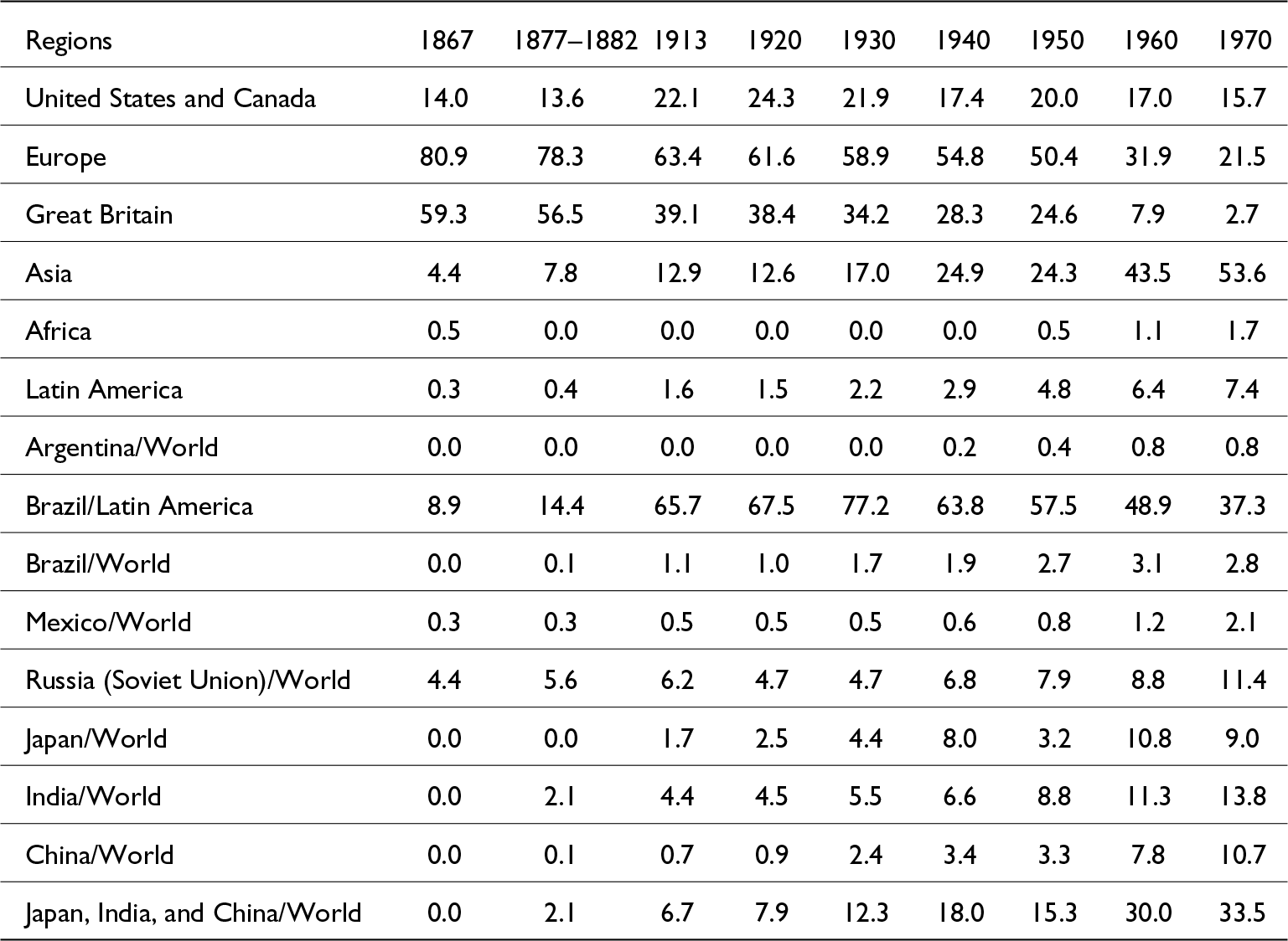
Before addressing these questions, let us examine the location of global investment in the textile industry from the late 19th century to the early 20th century in Table 1.

Table 1.

Cotton spindles in the world, Latin America, and Asia, in % quantity, 1867–1970

Table 1 Long description

The table reports each region’s percentage share of the world total number of cotton spindles across nine benchmark years from 1867 to 1970. Europe dominates early on, declining from 80.9% in 1867 to 21.5% in 1970; within Europe, Great Britain drops sharply from 59.3% to 2.7%. Asia grows steadily from 4.4% in 1867 to 53.6% in 1970, overtaking Europe by 1960 when Asia reaches 43.5% and Europe falls to 31.9%. The United States and Canada remain a secondary center, peaking at 24.3% in 1920 and ending at 15.7% in 1970. Latin America increases gradually from 0.3% to 7.4%, while Africa stays small, rising from 0.5% to 1.7% by 1970. Country shares highlight Asia’s rise: India reaches 13.8% and China 10.7% by 1970, while Japan peaks at 10.8% in 1960 and is 9.0% in 1970; the combined share of Japan, India, and China grows to 33.5% in 1970. Brazil’s share within Latin America is high but declines over time, from 77.2% in 1930 to 37.3% in 1970, while Brazil’s world share peaks at 3.1% in 1960 and is 2.8% in 1970. Values are percentages of totals, so they indicate distribution across regions and countries rather than absolute spindle counts.

Sources: Marson (Reference Marson2024), Appendix Table A1.

Despite a decline between 1867 and 1913, Europe still held two-thirds of all cotton spindles in the world until the start of the First World War. In 1867, Great Britain owned 60% of the world’s cotton spindles, a figure that had decreased to two-fifths by 1913. Despite the origins of mechanized spinning in the 19th century, Asia and Latin America had only 14.5% of the world’s cotton spindles in 1913, the largest being Russia with 6.2% and British India with 4.4%. Other economies, despite recent progress, could be described as infant industries, such as Japan with 1.7%, Brazil with 1.1%, China with 0.7%, and Mexico with 0.6% of the world’s cotton spindles in 1913. These figures changed rapidly from 1920Footnote ¹⁰ onward, with Asia overtaking US investment in cotton spinning in the 1930s and Europe in the 1950s. By 1970, Japan, India, and China owned 33.5% (9%, 13.8%, and 10.7%, respectively) of the world’s cotton spindles, and Latin America 7.4%, with Brazil holding 2.8% and Mexico 2.1%.

What explains these developments? Certainly, the relatively lower wages and less favorable working conditions partly explain the industry’s advance into Asia and Latin America. But these conditions, although not stable over time, were already relatively defined in the 19th century. Why did the transition to a low-wage economy not take place until after the First World War? A second hypothesis is that the decline in international trade in the interwar period provided the necessary protection for these countries to advance in their industrialization process. India, China, Argentina, and Brazil were major textile importers before the First World War. With the closure of the interwar economy, their industries would have turned to serving the large domestic market. Despite the importance of the interwar period, some forms of protection were already in place at the beginning of the 20th century.

What is proposed here is a new body of evidence on the costs of production in the global textile industry from the First World War onward. The hypothesis of the article is that as the cost of importing textile machinery rose between 1913 and the 1920s, economic incentives favored investment in regions where it was possible to increase the number of hours worked on machinery and equipment, thereby improving capital efficiency, and where it was also possible to increase the number of machines per operator, thereby improving labor efficiency. This investment was concentrated mainly in Asia and, to a lesser extent, in Latin America after the 1920s.

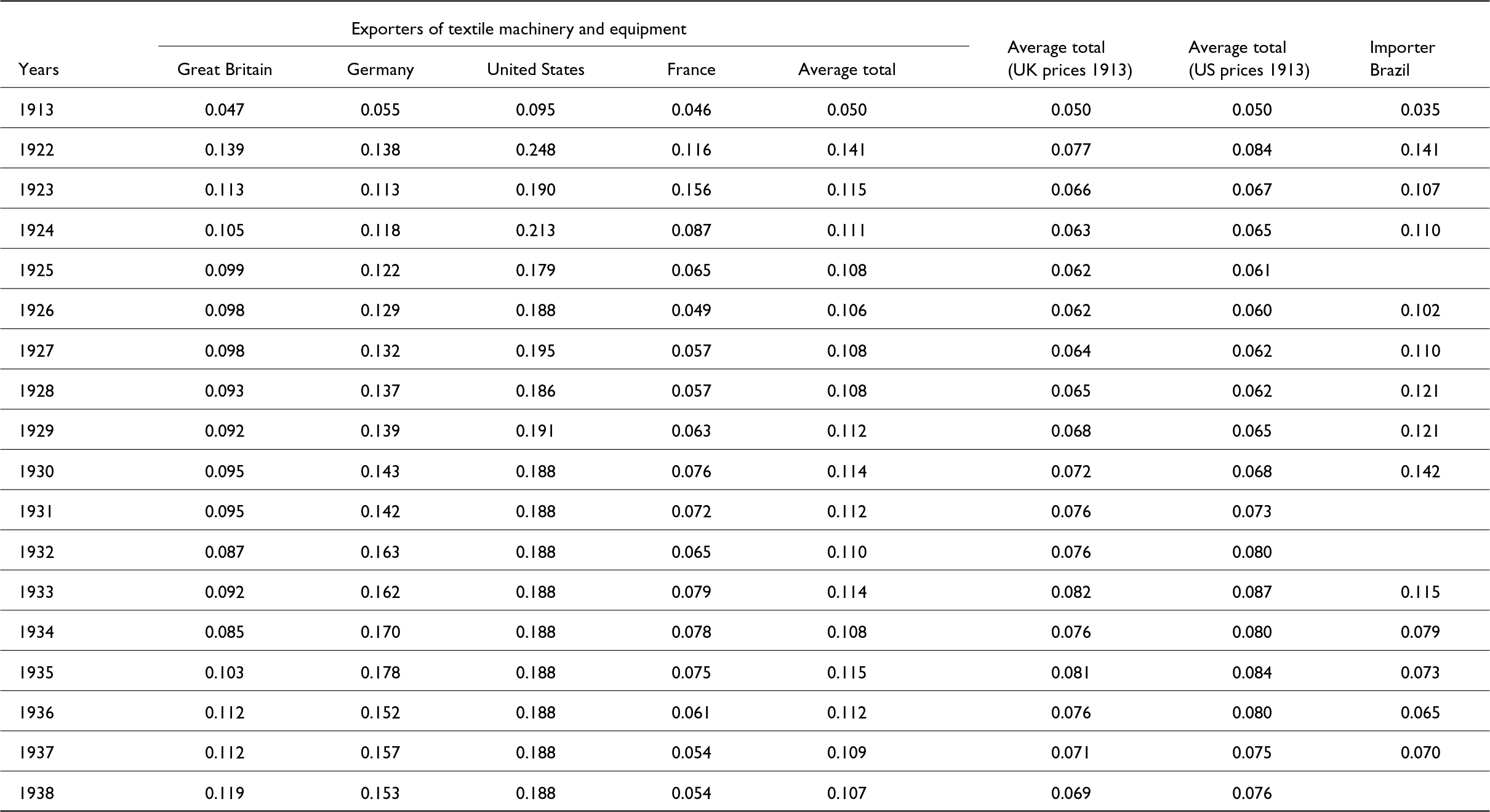
Much attention has been paid in the literature to the issue of labor, but little to the economic incentives associated with capital.Footnote ¹¹ Table 2 shows the evolution of the cost of capital, the average price of machinery and equipment in the textile industry between 1913 and 1938.

Table 2.

Price (£ per kg) of world exports (Great Britain, Germany, United States, France, and average total) and imports (Brazil) of textile machinery (for spinning and weaving, looms and their accessories), 1913–1938

Table 2 Long description

The table lists prices in pounds per kilogram for textile machinery exports from Great Britain, Germany, the United States, and France, plus an overall exporter average, alongside Brazil’s import price for selected years from 1913 to 1938. Export prices rise steeply from 1913 to 1922, when the exporter average reaches 0.141 and the United States peaks at 0.248, compared with 0.047 for Great Britain in 1913. After 1922, the United States remains consistently the most expensive exporter, holding at 0.188 from 1930 through 1938. Great Britain and France are generally the lowest-priced exporters, with Britain mostly around 0.085 to 0.119 in the 1930s and France declining to 0.054 in 1937 and 1938. Germany trends upward through the mid-1930s, reaching 0.178 in 1935 before easing to 0.153 by 1938. The overall exporter average stays near 0.106 to 0.115 from 1924 onward, ending at 0.107 in 1938. Two additional columns restate the exporter average in 1913 price terms using UK-based and US-based deflation; these real-price averages peak in 1933 at 0.082 and 0.087 and then fall to 0.069 and 0.076 by 1938. Brazil’s import price is 0.035 in 1913, rises to 0.141 in 1922, peaks at 0.142 in 1930, then drops markedly after 1933 to 0.079 in 1934 and 0.065 in 1936, with some years missing (for example 1925, 1931, 1932, and 1938).

Sources: Farnie (Reference Farnie1990, pp. 66–67); Cremer (Reference CREMER1926, pp. 4–5, 29 [1913–1924]); Brasil (1933), Comércio Exterior do Brasil, 1926–1930; and Brasil (1940), Comércio Exterior do Brasil, 1933–1937.

Note: Columns 7 and 8 of the table have been calculated using totals deflated by the UK and US cost of living indices from Mitchell (Reference Mitchell1992, pp. 846–851) and Mitchell (Reference Mitchell1983, pp. 841–845).

As Table 2 shows, the average price of exported textile machinery increased significantly between 1913 and 1922 (tripling from £0.05, one shilling, to £0.141, almost three shillings per kg). In real terms, machine export prices increased between 54% and 68% between 1913 and 1922, using the cost of living in the United Kingdom and the United States. The price of exported machinery rose in all exporting countries. Despite a slight fall in prices in the 1920s, there was a change in the average price level compared with the period of the First World War. On average, the real prices of exported textile machinery rose by around 40% between 1913 and 1938.

It seems that the machine price shocks of the 1910s and 1920s shifted the economic incentives and the global reorganization of textile industry production toward Asia.Footnote ¹² Why did this happen? In order to have an answer to this question, it is necessary to have some idea of a comparative estimate of the costs of the cotton textile industry around the world. Clark (Reference Clark1987) estimated manufacturing costs for numerous countries worldwide. We reestimated the manufacturing cost using the same methodology as Clark (Reference Clark1987) and added data for BrazilFootnote ¹³ (Table 3).

Table 3.

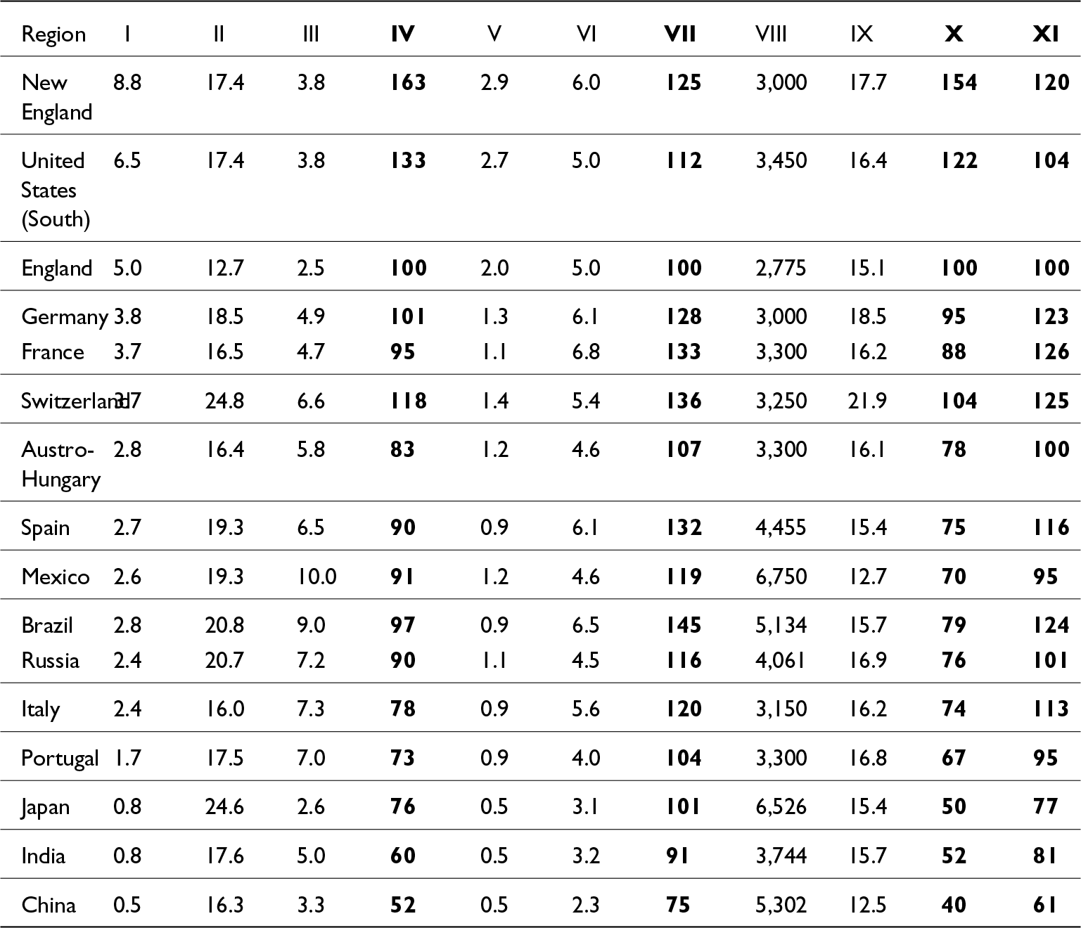
Cotton textile cost around the world, 1910

Table 3 Long description

The table compares cotton textile production inputs and cost indexes across regions, including wages, plant and machinery cost per spindle, coal price, machinery per worker, annual hours, and several manufacturing cost indexes benchmarked to England. Unadjusted manufacturing cost is highest in New England at 163 and lowest in China at 52, with England at 100. After adjusting for labour efficiency, Brazil rises to 145 and Switzerland to 136, while India falls to 91 and China to 75, indicating that differences in machines per worker materially change relative costs. After adjusting for capital efficiency, Japan drops to 50 and China to 40, while New England remains high at 154, reflecting the influence of operating hours and capital cost per spindle. When both labour and capital efficiency are considered together, the lowest cost indexes are China 61, India 81, Japan 77, and Mexico and Portugal at 95, while the highest are New England 120 and several European producers clustered around the mid 120s (France 126, Switzerland 125, Germany 123, Brazil 124). England and Austro-Hungary both end at 100 on the combined adjustment, while the United States South is slightly above at 104. Wages vary widely, from 8.8 in New England down to 0.5 in China, and annual hours range from 2,775 in England to 6,750 in Mexico, helping explain why capital-efficiency adjustments shift rankings. These figures are comparative indexes and recalculated estimates, so small differences should be treated as approximate rather than precise.

Source: Recalculated and adapted from Clark (Reference Clark1987, pp. 146, 148, 150–153).Footnote ¹⁴

Note: I—Weekly wage ($ 55 hours), II—Plant and machinery ($/spindle), III—Coal ($/ton), IV—Manufacturing cost (England = 100), V—Machinery per worker (loom equivalent), VI—Labor cost adjusted by machines per worker, VII—Manufacturing cost adjusted by labor efficiency (England = 100), VIII—Hours per year, IX—Cost of capital ($/spindle) adjusted by hours, X—Manufacturing cost adjusted by capital efficiency (England = 100), XI—Manufacturing cost adjusted for labor and capital efficiency (England = 100).

1. Data and sources for Brazil:

2. a) According to Versiani (Reference Versiani1993, p. 589), the wages earned by textile mill workers in Rio de Janeiro in 1920 were 5,600 réis per day. Adjusting for the cost of living between 1910 and 1920 using Lobo’s index (Lobo et al., Reference Lobo, Canavarros, Feres, Gonçalves and Madureira1971), this amounts to a value of 1,500 réis (equivalent to US$0.5) per day or US$2.8 per week (based on a 55-hour workweek) at 1910 prices.Footnote ¹⁵

3. b) The cost of capital was calculated based on the depreciation of 25% of the amount of capital (plants and equipment) per spindle in Brazil, using data from Stein (Reference Stein1979, p. 191). Clark (Reference Clark1987, p. 147) performed a similar calculation for the other countries.

4. c) The cost of coal for Brazil was calculated based on the average import price in 1912, which was valued at £1.85 (or U$ 9.01) per ton. This amounted to £4,299,000 per 2,318,210 tons (quoted at 1£ for US$4.87 in 1912). Source: Brasil (1916), Comércio Exterior do Brasil 1910–1914, p. XXXII.

5. d) In Brazil, mills claimed to operate 10 hours a day, 6 days a week at the end of the 19th century (Stein, Reference Stein1979, p. 73), but with the introduction of electric light the working day increased to 14–17 hours (52 weeks × 6 days = 312 days – 10 holidays = 302 days × 17 hours per day = 5,134 hours per year).

   The manufacturing cost was calculated using Clark’s methodology (Clark, Reference Clark1987, p. 146, Table 1). The cost was determined by the following proportion: (wage cost × 0.618) + (capital cost × 0.124) + (power cost × 0.034). This proportion represents the costs in England.

Table 3 presents the variables of the cost structure of the cotton industry worldwide in columns I, II, and III. Column I shows weekly wages for 55 hours of work, column II displays the cost of plants and machines per spindle, and column III shows the value of coal per ton, representing the costs of labor, capital, and power, respectively. There is a significant variation in wages between countries. In 1910, textile workers in the United States (New England and the South) and England received high wages, above US$5 per week. Germany, France, and Switzerland paid average wages between US$3.5 and US$4. Low-wage regions, such as the Austro-Hungarian Empire, Spain, Mexico, Brazil, Russia, Italy, and Portugal, paid between US$1.5 and US$3. Workers in Japan, India, and China received very low wages, between US$0.5 and US$0.8 per week. Workers in high-wage countries were paid over ten times more than workers in low-wage countries.

The cost of capital, as shown in column II, also varied between countries, although it was lower than wages. In 1910, England was the most cost-effective location for building cotton mills (US$12.7 per spindle) due to its large machinery and equipment industry for the textile sector. In 1910, the capital costs for building a cotton mill were highest in Switzerland and Japan, almost double that of England at over US$24 per spindle. Other countries, such as Russia, Brazil, Spain, and Mexico, also had high capital costs at around US$20 per spindle. Table 3, column III, shows that the cost of coal varies fourfold among the presented countries, with England being the least expensive at US$ 2.5 per ton, and Mexico and Brazil being the most expensive at US$ 10 and US$ 9 per ton, respectively.

The manufacturing cost estimate in column IV represents the total cost that would have been incurred by each country’s cotton industry if they had the same cost structure as the English industry (62% for wages, 12% for machine depreciation, 3% for power, and 22% for return on capital) and operated under the same conditions as in England, with mills open for 55 hours per week, the same amount of power per hour per steam boiler, and machines running at the same speed. The cost estimates for manufacturing in column IV show that all low-wage countries had a lower production cost than England and could compete in the open market for cotton textiles. However, it is important to note that these estimates do not take into account labor efficiency or capital efficiency, which can increase productivity by allowing workers to operate more machines and machines to work additional hours, respectively.

Gerschenkron (Reference Gerschenkron1962, pp. 8–9) notes that the low cost of labor argument can be viewed negatively or positively from the perspective of the industrialization of underdeveloped countries. In the case of the negative argument, the low cost of labor relative to capital goods emphasizes the consequent difficulty of substituting abundant labor for scarce capital. In the case of the positive argument, it is claimed that cheap labor in backward countries greatly facilitates industrialization processes. In fact, the real situation is more complex and varies across industries and countries.

Countries may use production inputs differently. In 1910, an English worker operated four times as many machines as a Japanese, Indian, or Chinese worker (column V, Table 3). The English worker was able to produce more goods per hour worked by operating more machines, which increased labor efficiency and reduced the cost of labor per unit produced in comparison to other countries. The machine-adjusted labor cost per worker is presented in column VI of Table 3. By comparing columns VI and I of Table 3, it is evident that regions with a higher machine-to-worker ratio than England, such as the United States, experience a decrease in the cost of labor. Conversely, regions with a lower machine-to-worker ratio than England, including all other countries, show an increase in the relative cost of labor.

Column VII of Table 3 estimates the manufacturing cost by adjusting the labor cost with the ratio of machines operated per worker. Based on labor efficiency estimates, only a few regions, such as China, India, and possibly Japan, would be able to compete with the production costs of the English cotton textile industry.

Furthermore, countries may use the machines and capital structures in mills differently. Regions with legislation restricting working hours may have incentives to use the capital structure less intensively, while regions with little labor protection tend to use machines and capital structures more intensively. The average number of hours that mills operated per year in each region is presented in column VIII of Table 3. In 1910, Mexico, Japan, and China had twice as many mill operating hours as England. Column IX of Table 3 estimates the cost of capital adjusted for mill operating hours. A comparison of columns IX and II shows that regions with a greater number of mill operating hours than England have a relatively lower cost of capital.

Column X of Table 3 estimates the cost of manufacturing by taking into account the efficiency of capital, i.e. by adjusting the cost of capital by the hours of operation of the mills. The estimates suggest that, considering the efficiency of capital, not only low-wage countries but also some high-wage countries such as Germany and France could have competed with the English cotton industry in 1910.

Column XI of Table 3 estimates the manufacturing cost of the cotton industry worldwide in 1910, considering both labor efficiency (machines operated per worker) and capital efficiency (mill operating hours). Based on estimates, only countries with low wages or high utilization of mill hours, such as China, India, Japan, Mexico, and Portugal, can compete with the costs of English cotton manufacturing. The economic benefits for capital were most prominent in Asian countries. During the First World War, the increased cost of textile machinery provided an incentive for the industry to relocate to regions where labor efficiency could be improved by increasing the number of machines operated per worker, and capital efficiency could be increased by intensifying the use of mill hours.Footnote ¹⁶

Therefore, it appears that the cost of capital and machinery played a more significant role than the quality of labor, particularly labor culture, in explaining the dynamics of the textile industry during the studied period. The following section examines Brazil’s case in this context.

4. Performance of the Brazilian cotton textile industry, 1870–1970

Why did the Brazilian cotton textile industry have a production cost estimated to be 24% higher than England and twice that of China in 1910 (Table 3, column XI), yet advanced from 1.1% of the world’s total spindles in 1913 to 3.1% in 1960 (Table 1)? The most direct answer lies in tariff protectionFootnote ¹⁷ and the relative closure of the domestic market to imports during the interwar period, coupled with currency devaluation. The average tariff on manufactured imports in Brazil was 60%, while in Japan it was 28%, in China 5%, and in India 4% in 1913 (Williamson, Reference Williamson2011, p. 219; Findlay and O’Rourke, Reference Findlay and O’Rourke2007, p. 403). What were the consequences of protected growth on the productivity of the Brazilian textile industry?

Before attempting to answer these questions, it is essential to comprehend the reasons behind Brazil’s high manufacturing costs compared to its global competitors in 1910. As shown in Table 3, Brazil’s cotton textile industry paid just over half the wage (column I), had a capital cost, with mills and equipment, almost double (column II), and a power cost 3.6 times higher than that of England in 1910. As we have seen, the literature has established the costs of labor and power, but little attention has been paid to the cost of capital.Footnote ¹⁸ The reason for such a high cost of capital is unclear. Additionally, why did the construction of cotton textile mills in Brazil cost significantly more than in England and other places? Has the cost of capital in the Brazilian textile industry always been higher than in England?

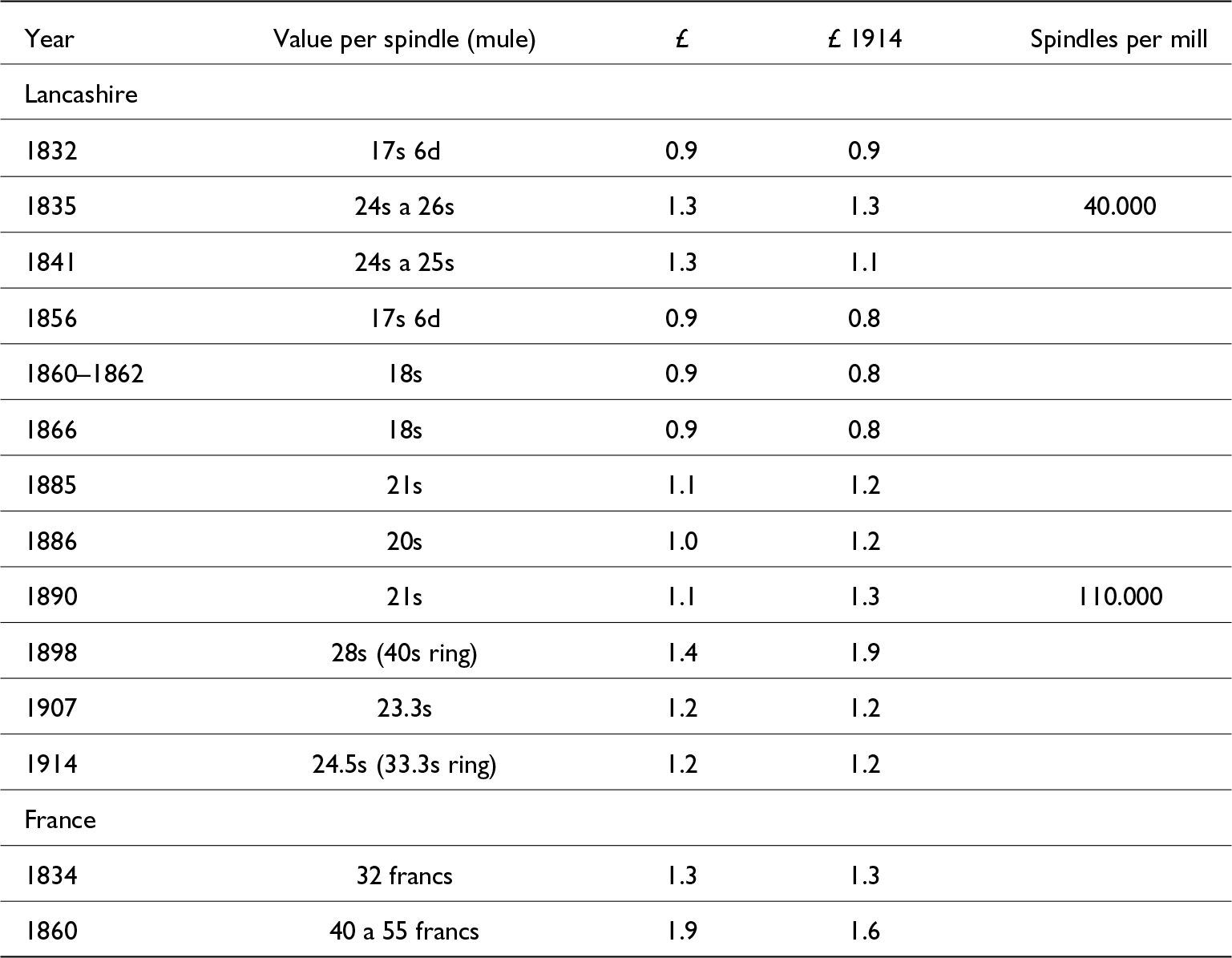
Firstly, it is informative to consider the initial cost of a mill in developed regions. Table A1, in the Appendix, presents the initial cost of mills in Lancashire and France during the 19th and early 20th centuries. The initial cost of a mill in Lancashire ranged from £0.9 to £1.4 (or £0.8 to £1.9 in 1914 values) per spindle between 1832 and 1914. In France, the initial cost of a mill was slightly higher, ranging from £1.3 to £1.9 (or £1.3 to £1.6 in 1914 values) per spindle between 1834 and 1860.

At the outset of the Industrial Revolution in the 18th century, the initial investment required for a cotton mill was relatively modest, ranging from £2,000 to £4,000, equally divided between fixed and working capital. Samuel Greg’s Quarry Bank Mill, for instance, had an initial cost of £3,000 in the 1780s. From 1800 onward, there was a significant increase in the demand for fixed capital due to the implementation of Boulton & Watts’ steam engines and the spread of the spinning mule (invented by Crompton in 1779) (Toms, Reference Toms2020, p. 17; Beckert, Reference Beckert2014, p. 62; Berg and Hudson, Reference Berg and Hudson2023, p. 156). However, according to Berg and Hudson (Reference Berg and Hudson2023, p. 44), the average capital of cotton mills in England in 1805 was £5,000. In 1814, Quarry Bank Mill was valued at £20,000. Samuel Greg’s Peter Street Mill, built in Manchester in 1806, cost £44,355 (Toms, Reference Toms2020, p. 51). During the 1830s and 1840s, the main mills had fixed capital ranging from £30,000 to £60,000. For instance, Ashworth Brothers’ New Eagley Mill had a fixed capital of £38,526 in 1831, Fielden Brothers’ Waterside Mill had a fixed capital of £61,000 in 1832, and Joseph Jones’ Wallshaw Mill had a fixed capital of £30,742 in 1847 (Toms, Reference Toms2020, pp. 56–59).

In the 1860s and 1870s, start-up capital for new large English mills ranged from £50,000 to £100,000 (Toms, Reference Toms2020, p. 133, note 53). Additionally, the average number of spindles per mill increased from 40,000 in 1835 to 110,000 in 1890 (Table A1).

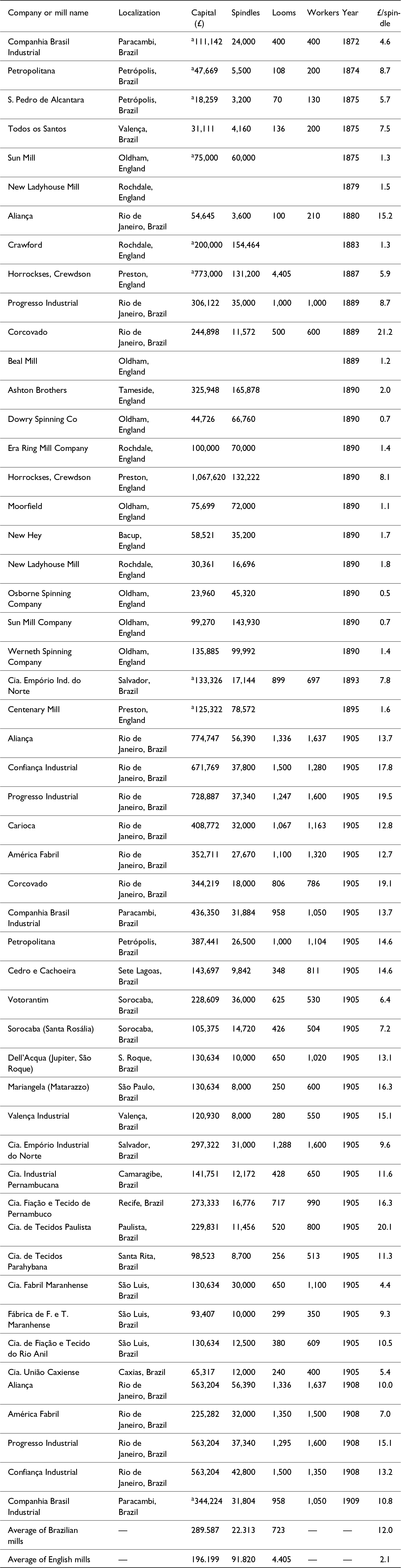
Comparing the cost of mills between countries in different periods is a challenging task. However, Table A2, in the Appendix, provides an overview of the differences in the cost of capital and other relevant information, such as the number of spindles and looms, between English and Brazilian cotton mills from 1870 to 1910. The initial mechanized cotton mills in Brazil were established during the second quarter of the 19th century, specifically in Bahia and Rio de Janeiro in the Northeast and Southeast, respectively. However, the expansion of the mills only gained momentum in the final quarter of the 19th century.

In the 1840s, the largest mills, such as Todos os Santos in Valença, Bahia, had an initial fixed cost of 220 contos de réis (equivalent to £24,229 in 1848) (Santos, Reference Santos2023, pp. 157, 165), which was close to the English mills. However, the Brazilian mill (Todos os Santos) was much smaller in terms of machines (2,000 spindles and 50 looms), as well as workers (between 80 and 120).Footnote ¹⁹

The Companhia Brasil Industrial Mill was constructed in Fazenda de Macacos, now Piracambi, Rio de Janeiro, in 1872. The total cost of the project was 1,088 contos de réis (£111,142), which included the purchase of land, buildings, infrastructure, railway branch, machinery installation, freight, and taxes. The equipment cost constituted 45% of the total cost of the mill (Stein, Reference Stein1979, p. 45). As we have seen, the cost of constructing an English cotton mill during this period ranged from £50,000 to £100,000. Despite having a construction cost similar to that of an English mill, Companhia Brasil Industrial Mill had significantly fewer pieces of equipment, with only 24,000 spindles. This is in contrast to the average number of spindles in English mills, which ranged from 50,000 to 100,000 (equivalent to £0.9 to £1.1 per spindle between 1866 and 1885, as shown in Table A1). For instance, in 1875, Sun Mill, situated in Oldham, had a fixed capital of £75,000 and 60,000 spindles (equivalent to £1.3 per spindle). New Ladyhouse Mill, located in Rochdale, had a capital per spindle of £1.5 in 1879, while Crawford Mill had £1.3 in 1883. Table A2 shows that Companhia Brasil Industrial Mill had a capital per spindle almost four times higher, at £4.6.

Table A2 shows the difference in spindle capital costs between Brazilian and English mills from 1870 to 1910. The data indicate that, despite some fluctuations, the initial cost of installing a cotton mill in Brazil was significantly higher than in England.Footnote ²⁰ Although the construction costs of the total mills were similar, the amount of machinery and equipment was much smaller in Brazil. Therefore, the cost of building a mill in Brazil was already high prior to the First World War. The mills in Brazil were designed similarly to those in England, resulting in significantly higher equipment costs. One potential explanation for this difference is the varying demand between Brazilian and English mills. Although English mills faced competition and required a large scale of production, Brazilian mills did not have the same demand for such a scale of production.

Upon viewing photographs or entering an old Brazilian textile mill building from the late 19th and early 20th centuries, one may observe striking similarities to English mills from the same era. The building’s design, construction, machinery, equipment, technicians, and managers all reflect the English style of the time. In other words, the technological transfer took place, but at a higher initial capital cost and with low productivity in the long term.

The primary source to investigate the high initial capital required to construct a cotton textile mill in Brazil is the machinery and equipment market. It is possible that the British machinery industry sold textile equipment to Brazil at a higher price than to the domestic market and other countries. However, Table 2 shows that this hypothesis cannot be confirmed. The average price of textile machinery and equipment imported by Brazil was similar to the average prices exported worldwide and by the British.

There were many expenses, from ordering the equipment abroad to getting the mill up and running. Although the selling price of the machinery and equipment was relatively close to the price paid on the international market, the Brazilian mills had to pay for freight (between 7% and 25% of the value of the equipmentFootnote ²¹), port costs (5%Footnote ²²), the hiring of technicians and materials to install the machinery (20%Footnote ²³), customs duties (36%Footnote ²⁴), and the commission of the import houses. The import houses were essential in the technology transfer process and often also acted as financiers of the equipment imports, making it difficult to determine the true value of the commission. In addition to all these fees, there was also the foreign exchange risk in the equipment transaction.

Import tariffs were levied partly in gold and partly in paper money (Clark, Reference CLARK1910, p. 25; Cremer, Reference CREMER1926, pp. 12–14). According to Cremer (Reference CREMER1926, p. 13), 60 percent of customs tariffs had to be paid in gold. The ratio between mil réis gold and mil réis paper was around 3.5 paper currency for every mil réis gold (in 1910, mil réis gold was worth 3.33 paper mil réis, Law 2359 of December 31, 1910).

Imports of textile machinery are classified in class 34 of the Customs Tariff as “machinery for mills or workshops” and have a 15% ad valorem tariff in 1914. If the tariff charged is 60 percent in gold and 40 percent in paper money of one mil réis, the customs tariff will be charged as follows: (0.6 × 3.33 × 0.15 × x) + (0.4 × 0.15 × x) = 0.2997x + 0.06x = 0.3597x, where x is the import value of the machine. The 15 percent tariff on the value of the machine or equipment will be increased by 36 percent, resulting from the 60 percent tariff in mil réis gold. An import tax of 36% will be levied on the import value of the machine (x).

Thus, estimates suggest that the additional cost of the machinery and equipment to run the mill is about 68 percent (7% freight, 5% port costs, 20% installation costs, and 36% duty) over the value of the imported machinery. These estimates are close to the average additional value of 64 percent of the cost in dollars per spindle between Brazil (US$ 20.8) and England (US$ 12.7) in 1910 (Table 3, column II).

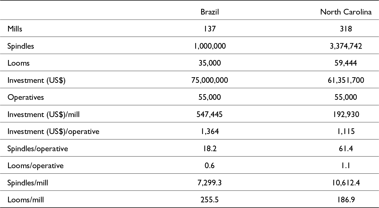
Until 1910, the initial cost of a textile mill in Brazil was higher than in England, but also higher than in one of the major manufacturing regions in the United States at the time, North Carolina.Footnote ²⁵ Table 4 compares the cotton textile industries of Brazil and North Carolina in 1910. The data show that North Carolina’s industry was approximately three times larger than Brazil’s, in terms of the number of mills and spindles. However, both regions had an equal number of workers, and investment in Brazil was relatively higher.Footnote ²⁶

Table 4.

Cotton textile industry in Brazil and North Carolina (United States), 1910

Table 4 Long description

The table compares the cotton textile industry in Brazil and in North Carolina in 1910 using counts of mills, spindles, looms, investment, and several per mill and per worker ratios. North Carolina had more mills, 318 versus 137, and many more spindles, 3,374,742 versus 1,000,000, along with more looms, 59,444 versus 35,000. Total investment was higher in Brazil at 75,000,000 US dollars compared with 61,351,700 US dollars in North Carolina. Both places report the same number of operatives, 55,000, but North Carolina shows much higher equipment per worker, with 61.4 spindles per operative versus 18.2 in Brazil and 1.1 looms per operative versus 0.6. Investment per mill is higher in Brazil, 547,445 US dollars per mill versus 192,930, and investment per operative is also higher in Brazil, 1,364 versus 1,115. Per mill capacity differs by measure: North Carolina has more spindles per mill, 10,612.4 versus 7,299.3, while Brazil has more looms per mill, 255.5 versus 186.9. These figures are a snapshot for one year and rely on the source definitions of investment and operatives, so differences may reflect reporting practices as well as industrial structure.

Source: Clark (Reference CLARK1910), p. 46.

Investment per mill in Brazil was 2.8 times higher than in North Carolina, and investment per worker was 20% higher in Brazil. Furthermore, workers in North Carolina operated 3.4 times more spindles and 70% more looms than workers in Brazil. On average, the mills in North Carolina had 50% more spindles than those in Brazil but operated fewer looms (70%).

In 1910, North Carolina had a higher production capacity than Brazil, measured in mills and spindles, with greater labor productivity, more spindles and looms per operator, and lower investment costs.

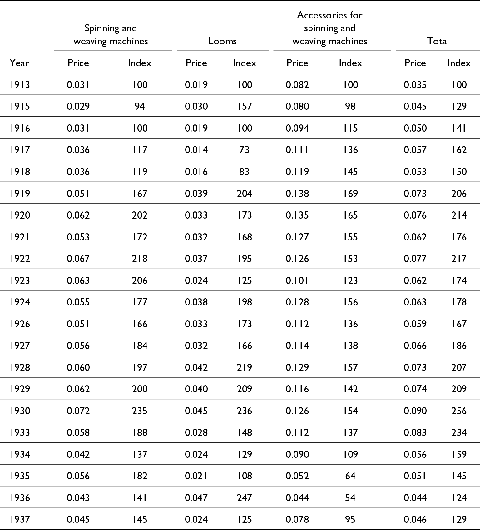
The outbreak of the First World War resulted in an increase in the cost of investing in textile mills worldwide, as demonstrated by the data in Table 2. This increase was particularly significant for Brazil. Table 5 provides details of the prices (£ per kg) of imported spinning and weaving machinery, looms, accessories, and the total cost of all machinery and equipment between 1913 and 1937. From 1919 onward, prices for all textile machinery and equipment more than doubled compared to 1913 and remained at this level until 1922.Footnote ²⁷ Although there was a slowdown in prices between 1923 and 1927, they increased again between 1928 and 1933. Only after 1933 did machine prices begin to fall, possibly due to the import of used and second-hand machines from developed countries. Even with the crisis, machine prices in the 1930s remained significantly higher than those of the pre-World War I period.

Table 5.

Brazil’s import price (£ per kg) of textile machinery (for spinning and weaving machines, looms, and their accessories), in 1913 prices and index, 1913–1937

Table 5 Long description

The table reports Brazil’s import prices per kilogram in pounds sterling for textile machinery, shown as inflation-adjusted prices and index values with 1913 as the base year. It breaks results into spinning and weaving machines, looms, accessories, and an overall total for selected years from 1913 to 1937. Overall prices climb from the 1913 base to a postwar high in 1919 to 1922, with the total index reaching 206 in 1919 and 217 in 1922. The highest overall level occurs in 1930, when the total price is 0.090 and the index is 256. After 1930 the total declines, reaching its lowest point in 1936 at 0.044 and index 124, then rises slightly in 1937 to 0.046 and index 129. Category patterns differ: looms are volatile, with a low index of 73 in 1917 and a high of 247 in 1936, while accessories peak earlier at index 169 in 1919 and fall to 54 in 1936. Because values are adjusted using a UK cost-of-living measure, the series is best read as changes in real import prices rather than nominal prices in Brazil.

Sources: Cremer (Reference CREMER1926, pp. 4–5, 29); Brasil (1921), Comércio Exterior do Brasil, 1913–1918, pp. 216–218; Brasil (1924), Comércio Exterior do Brasil, 1919–1923, p. 58; Brasil (1933), Comércio Exterior do Brasil, 1926–1930, pp. 249–252; and Brasil (1940), Comércio Exterior do Brasil, 1933–1937, pp. 434–436.

Note: The prices were adjusted for inflation using the UK cost of living index Mitchell (Reference Mitchell1992, pp. 846–851).

Certainly, the slowdown in the prices of textile machinery and equipment explains the increase in the capacity of the textile industry between 1923 and 1927, with investments being made using profits accumulated during the First World War (Fishlow, Reference Fishlow1972, p. 20; Versiani and Versiani, Reference Versiani, Versiani, Versiani, DE Barros and R.1977, pp. 138–140). Most of the literature treats currency appreciation throughout the 1920s, especially between 1923 and 1926, as the main incentive for reducing the cost of imported machinery and expanding installed capacity. However, the data used to infer the reduction in cost is the “value” of imports of textile machinery and equipment, an approximation of the value of industrial investment, indicating an increase in investment value and not a lower cost (see Suzigan, Reference Suzigan2000, pp. 159–161). In reality, the quantity of machinery imported for these investments was more expensive than in the period prior to the First World War, as shown in Table 5.

One explanation for the increase in investment and installed capacity, even during a period of crisis, from 1923 onward, is that new production plants and equipment were essential for expanding and maintaining market share, as they enabled more efficient production at lower costs. Consequently, the economic downturn experienced in the latter half of the 1920s had a disproportionately adverse impact on companies utilizing outdated equipment, particularly in Bahia and the Federal District (Versiani and Versiani, Reference Versiani, Versiani, Versiani, DE Barros and R.1977, p. 139; Versiani, Reference Versiani1972, pp. 23–25). The renewed increase in the prices of imported machinery and equipment between 1928 and 1933 probably meant that the production costs of old equipment were lower than the total costs of new equipment (production costs, plus the cost of purchasing new machinery), according to Versiani (Reference Versiani1972, pp. 43–44), indicating a decision to replace equipment more slowly and keep obsolete equipment for a longer period.

What was the impact of the increase in machinery and equipment prices on the textile industry in Brazil after the First World War? One consequence was that it became more expensive to renovate and modernize mills. Another consequence was the emergence of an incipient capital goods industry to replace imported machines by copying and reverse engineering foreign equipment. The production of spare parts and equipment for textile machines has been a common practice in the mechanical workshop of textile mills since the late 19th century (Stein, Reference Stein1979, p. 52). However, the rise in prices during World War I led to the emergence of an industry that specializes in textile machinery.

Although the production of the first national loom by Ribeiro Brothers in 1920 was a landmark of this period, other companies also expanded their production of textile machinery. These companies include Vagnotti, founded in 1900 to produce parts, Paulo Andrighetti & Brothers, founded in 1922, Pedro Pozzi, founded in 1925, and Coltro Brothers, founded in 1926 (Marson, Reference Marson2017, pp. 112–121). In the 1950s, the Ribeiro Brothers became the largest loom manufacturers in Latin America (Stein, Reference Stein1979, pp. 148, 251, note 33). During the 1920s, América Fabril, Brazil’s primary textile industry located in Rio de Janeiro, produced spare parts for machine repairs, a practice that began during the First World War. In subsequent years, the company began constructing complete machines by replicating British models. The machines named “Independência” and “Liberdade” during the Great Cotton Textile Exhibition, in celebration of Brazil’s centenary in 1922, were the most complex and delicate machines used in cotton spinning (von der Weid and Bastos, Reference von der Weid and Bastos1986, p. 149).

The increase in import prices after the First World War certainly led to the expansion of Brazilian textile machinery production. However, due to the machinery industry’s dependence on imported technology and its incipient nature, the most significant long-term consequence of this structural change was its impact on the productivity of the Brazilian textile industry. Expanding and renovating the mills was expensive.Footnote ²⁸

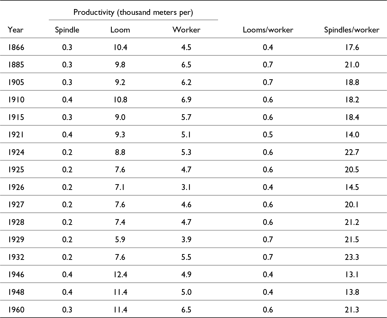
As Table 6 shows, both capital productivity (meters produced per spindle and loom) and labor productivity (meters produced per worker) in the Brazilian cotton textile industry were lower than in 1910 until the 1940s. Only in 1946 and 1948 does capital productivityFootnote ²⁹ exceed the 1910 level. In 1960, labor productivity was at a level that was lower than that experienced during the period preceding the First World War.Footnote ³⁰

Table 6.

Productivity indicators in Brazil’s cotton textile industry, 1866–1960

Table 6 Long description

The table reports cotton textile productivity in Brazil from 1866 to 1960, measured as thousand metres produced per spindle, per loom, and per worker, plus equipment intensity as looms per worker and spindles per worker. Output per spindle stays low and fairly stable, ranging from 0.2 to 0.4, with higher values in 1910, 1921, 1946, and 1948. Output per loom declines from 10.4 in 1866 to a low of 5.9 in 1929, then rebounds strongly to 12.4 in 1946 and remains high at 11.4 in 1948 and 1960. Output per worker varies from 3.1 in 1926 to 6.9 in 1910, ending at 6.5 in 1960. Looms per worker ranges from 0.4 to 0.7, with higher levels in 1885, 1905, 1929, and 1932, and lower levels in 1866, 1926, 1946, and 1948. Spindles per worker ranges from 13.1 in 1946 to 23.3 in 1932, with relatively high values again in 1960 at 21.3. Because the measures mix output rates and staffing intensity, changes over time may reflect technology, utilization, product mix, or labor organization rather than a single cause.

Sources: Calculated based on Stein (Reference Stein1979, p. 191) and CEPAL (1962, pp. 14–16, 82).

The low level of labor productivity is explained by the low ratio of looms per worker, which increased between 1929 and 1933, due more to the decline in the number of workers as a result of the crisis than to the increase in the number of machines. The indicator of spindles per worker performed better, but the increase was relatively small, and the improvement occurred during a period of crisis in the textile industry, which may reflect a decline in the number of workers rather than an increase in the number of spindles.

Low labor productivity may be explained by the high cost of importing equipment, as shown in Table 5.Footnote ³¹ The fact that the price of imported textile machinery virtually doubled in the 1920s and 1930s may have had an impact on capital productivity, adding to the already high costs of investment and plant renewal in the cotton textile sector.