1 Introduction
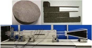
Acoustic liners (Tester Reference Tester1973; Rienstra & Eversman Reference Rienstra and Eversman2001; Zhang & Bodony Reference Zhang and Bodony2016) remain the most effective device in controlling aeroengine noise emissions from the inlet and bypass flow ducts (Huang et al. Reference Huang, Chen, Ma and Zhang2008; Zhang Reference Zhang2012; Liu, Huang & Zhang Reference Liu, Huang and Zhang2014). Increasing attention is being paid to new materials, such as granular porous metals, composite materials and cloaking metamaterials (Huang, Zhong & Liu Reference Huang, Zhong and Liu2014), which will enable new liner designs that could possibly provide high sound absorption over a broad range of frequencies (Zhao et al. Reference Zhao, Liu, Zhao and Grosh2014). A photo of one such new liner material is shown in figure 1. The randomly woven fibrous structure of the material is clearly visible in the photo. This kind of structure has variable density which could lead to a non-uniform acoustic impedance distribution in the resulting liner, which requires new analysis methods. To address this demand, the current work proposes a theoretical model for liners which are semi-infinite in the axial direction with variable acoustic impedance values in the azimuthal direction. Axial rigid splices, as a special case of azimuthally non-uniform liners, have been examined by using either numerical simulations (McAlpine & Wright Reference McAlpine and Wright2006; Wright & McAlpine Reference Wright and McAlpine2007) or analytical methods, such as mode matching (Fuller Reference Fuller1984), the Green’s function approach based eigenmodes analysis (Brambley, Davis & Peake Reference Brambley, Davis and Peake2012) and the Wiener–Hopf method (Liu et al. Reference Liu, Jiang, Huang and Chen2015). A more generic set-up with azimuthally non-uniform impedance values has been studied by using the superposition of eigenfunctions method (Campos & Oliveira Reference Campos and Oliveira2004, Reference Campos and Oliveira2013) and some possible benefits in terms of noise attenuation by the variable impedance have been suggested.
An example of a new liner material, which has a randomly woven fibrous structure. The associated impedance can be further controlled by the variable material thickness. The preliminary impedance eduction experiments (Jiang & Huang Reference Jiang and Huang2017a ) conducted in our group with a grazing flow impedance tube at HKUST have confirmed the associated non-uniform impedance properties. This material can be put in isolated cells (see top right) to achieve local impedance.

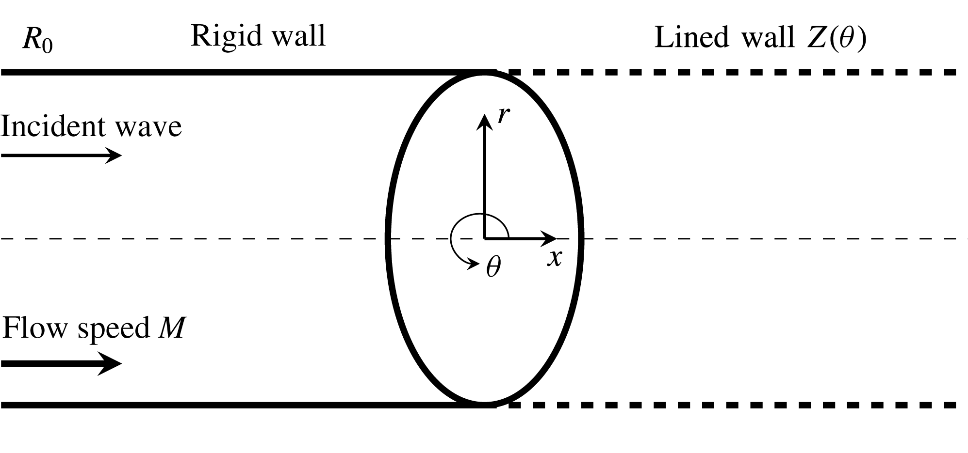
In this work, we consider a set-up with axially semi-infinite, azimuthally non-uniform lined wall (see figure 2), which is a progressively more complicated set-up than those in previous studies (Rienstra & Eversman Reference Rienstra and Eversman2001; Liu et al. Reference Liu, Jiang, Huang and Chen2015). For finite-length liner set-ups, Koch & Möhring (Reference Koch and Möhring1983) have developed eigensolutions for a rectangular duct. Our new theoretical model is developed by heavily extending the essential concept developed in Liu et al. (Reference Liu, Jiang, Huang and Chen2015) that incorporates Fourier series expansion into the Wiener–Hopf method. The latter is a beautiful mathematical tool for solving wave problems in fluids and acoustics (Noble Reference Noble1958), amongst which the flow duct cases are likely the most relevant to practical aerospace applications. One of the earliest examples of the use of the Wiener–Hopf method for duct acoustics is that by Munt (Reference Munt1977), who studied the semi-infinite hollow cylinder case with a shear layer by using the scalar Wiener–Hopf model. Then, Gabard & Astley (Reference Gabard and Astley2006) considered the extended configuration of a flow duct with an infinite centre body. Veitch & Peake (Reference Veitch and Peake2008) further examined the set-up with a finite centre body by using the more complicated matrix Wiener–Hopf model. Rienstra (Reference Rienstra2007) analysed the scattering and attenuation of a downstream-propagating wave at the hard–soft interface for flow duct cases with semi-infinite lined walls. Our recent work has further considered semi-infinite axial liner splices (Liu et al. Reference Liu, Jiang, Huang and Chen2015) and proposed the corresponding Wiener–Hopf model with a specialised matrix kernel.
Sketch of the model problem in cylindrical coordinates
 $(x,r,\unicode[STIX]{x1D703})$
. The axial
 $x$
-coordinate is aligned with the central axis and is parallel to the walls. The
 $r$
-direction is normal with respect to the walls at
 $r=\pm R_{0}$
. The left half-semi-infinite wall (
 $x<0$
) is rigid and the right half-semi-infinite wall (
 $x>0$
) is lined with an azimuthally non-uniform impedance
 $Z(\unicode[STIX]{x1D714},\unicode[STIX]{x1D703})$
.

In this work, we further extend the previous work by proposing a more mathematically rigorous matrix factorisation for more generic, axially non-uniform set-ups. In particular, we propose a mathematical method to solve residues related to the so-called pole-removal technique, which enables full matrix kernel factorisation. More specifically, the essential step in the Wiener–Hopf method is the factorisation of a kernel function. For example, provided a kernel
 $\mathscr{K}$
, its multiplicative factorisation seeks the decomposed pairs
 $\mathscr{K}_{\pm }$
that satisfies
 $\mathscr{K}_{-}\mathscr{K}=\mathscr{K}_{+}$
, where
 $\mathscr{K}_{\pm }$
are analytic, invertible and show algebraic behaviour at infinity. For those relatively simple flow duct problems (Munt Reference Munt1977; Gabard & Astley Reference Gabard and Astley2006; Rienstra Reference Rienstra2007), the relevant Wiener–Hopf kernels are scalar functions and the corresponding factorisations can be straightforwardly obtained by using Cauchy type integrals (Noble Reference Noble1958). However, to the best of our knowledge, a generic factorisation method for matrix kernels is still not available. This obstacle has been bypassed in our previous work (Liu et al.
Reference Liu, Jiang, Huang and Chen2015) by approximating the resultant matrix kernel using a diagonal matrix, which appears to be appropriate for the specialised lined splice set-up. In this work, we consider a more generic (and complicated) set-up with axially semi-infinite, azimuthally non-uniform impedance values and propose a rigorous theoretical model by using the pole-removal technique (Abrahams Reference Abrahams1987; Veitch & Peake Reference Veitch and Peake2008) that does not require any substantial approximation. More specifically, the pole-removal technique will subtract residue contributions from a meromorphic function (formed from elements of a kernel matrix
 $\mathscr{K}$
) to achieve the desired analytic property (Idemen Reference Idemen1979). The same technique is applied in this work and an intricate way is proposed to solve the unknown residues. The convergence of residues is also studied in this work. Then, we use the proposed model to study azimuthally non-uniform set-ups with either piecewise uniform impedance or sinusoidal-type impedance, and the noise-absorbing performance of these azimuthally non-uniform liners is discussed. Therefore, the contribution of the current work is twofold: (i) to enhance the theoretical modelling capability for progressively more complicated set-ups of practical importance, and (ii) to illuminate the physical mechanism of sound wave scattering from the axial hard–soft interface and the azimuthally non-uniform lined walls.
The remaining part of this paper is organised as follows. The governing differential equations and boundary conditions for the derivation of the current analytical model are described in § 2. Although this part is superficially similar to that of our previous work (Liu et al. Reference Liu, Jiang, Huang and Chen2015), it actually requires a more intricate treatment. Therefore, the differences from our previous work and the innovative aspects of our current model will be highlighted and discussed in § 2. Then, the mathematically tricky solution part will be presented in § 3. After that, the proposed analytical model will be validated by comparing to several representative numerical cases in § 4. A couple of special azimuthally non-uniform set-ups with impedance values of representative segmental and sinusoidal distributions will be analysed by using this model in § 4. Finally, § 5 concludes the present work.
2 The current theoretical model
This work considers sound scattering in a lined duct that contains a uniform background flow. Boundary layer and vorticity are omitted to enable the theoretical development in the framework of the Wiener–Hopf method. By assuming much larger time scale and length scale of fluid dynamics than the corresponding scales of acoustic waves, the sound wave propagation and scattering should satisfy the convective wave equation, such that
 $$\begin{eqnarray}\left(\frac{\unicode[STIX]{x2202}}{\unicode[STIX]{x2202}t}+M\frac{\unicode[STIX]{x2202}}{\unicode[STIX]{x2202}x}\right)^{2}\unicode[STIX]{x1D719}-\unicode[STIX]{x1D6FB}^{2}\unicode[STIX]{x1D719}=0,\quad r<\unicode[STIX]{x1D709}_{s}(x,\unicode[STIX]{x1D703},t),\end{eqnarray}$$
where
 $\unicode[STIX]{x1D719}$
is the acoustic potential,
 $M$
is the Mach number of the uniform background flow and
 $\unicode[STIX]{x1D709}_{s}=\unicode[STIX]{x1D709}_{s}(x,\unicode[STIX]{x1D703},t)$
is the kinematic displacement of the hypothetical infinitely thin vortex sheets developing along the lining surfaces (Rienstra Reference Rienstra2007). In the following discussion, all variables are non-dimensionalised using the mean flow density
 $\unicode[STIX]{x1D70C}_{0}$
, the speed of sound
 $c_{0}$
and the duct radius
 $R_{0}$
. As shown in figure 2, we have a circular duct with a unit outer radius, a hard wall along
 $x<0$
and a lined wall for
 $x>0$
with azimuthally non-uniform impedance
 $Z(\unicode[STIX]{x1D714},\unicode[STIX]{x1D703})$
(normalised by
 $\unicode[STIX]{x1D70C}_{0}c_{0}$
). In our previous work (Liu et al.
Reference Liu, Jiang, Huang and Chen2015),
 $Z(\unicode[STIX]{x1D714},\unicode[STIX]{x1D703})$
is infinite for the rigid splices and is a finite constant for the lined wall. Therefore, the associated distribution along the azimuthal direction was a rectangular Pi function, and it was possible to adopt a manipulation to simplify the relevant matrix kernel factorisation (Liu et al.
Reference Liu, Jiang, Huang and Chen2015). In contrast, a more generic set-up with
 $Z(\unicode[STIX]{x1D714},\unicode[STIX]{x1D703})$
being any arbitrary function of
 $\unicode[STIX]{x1D703}$
is considered in this paper, which calls for a more rigorous mathematical treatment.
First, we build up the mathematical model and assume the acoustic field with angular frequency
 $\unicode[STIX]{x1D714}$
has the following relations:
 $$\begin{eqnarray}p=p_{i}+p_{s}=\left(\text{i}\unicode[STIX]{x1D714}\unicode[STIX]{x1D719}-M\frac{\unicode[STIX]{x2202}\unicode[STIX]{x1D719}}{\unicode[STIX]{x2202}x}\right),\quad \boldsymbol{v}=\unicode[STIX]{x1D735}\unicode[STIX]{x1D719},\quad \unicode[STIX]{x1D70C}=p,\end{eqnarray}$$
where
 $(\cdot )_{i}$
and
 $(\cdot )_{s}$
represent the incident and scattered wave fields, respectively. From the generic solution of duct acoustics, the tonal and axisymmetric incident field inside a cylindrical duct has the form:
 $$\begin{eqnarray}\unicode[STIX]{x1D719}_{i}(x,r,\unicode[STIX]{x1D703},t)=\unicode[STIX]{x1D713}_{i}(x,r)\text{e}^{\text{i}m\unicode[STIX]{x1D703}-\text{i}\unicode[STIX]{x1D714}t}=\text{J}_{m}(\unicode[STIX]{x1D6FC}_{mn}r)\text{e}^{\text{i}\unicode[STIX]{x1D714}\unicode[STIX]{x1D707}_{mn}^{+}x}\text{e}^{\text{i}m\unicode[STIX]{x1D703}-\text{i}\unicode[STIX]{x1D714}t},\end{eqnarray}$$
where
 $m$
is the circumferential mode number and
 $\text{J}_{m}$
is the
 $m$
th-order Bessel function of the first kind;
 $\unicode[STIX]{x1D6FC}_{mn}$
is the
 $n$
th solution of the characteristic equation
 $\text{J}_{m}^{\prime }(x)=0$
for the hard wall; and
 $\unicode[STIX]{x1D707}_{mn}^{+}=(\sqrt{1-(1-M^{2})\unicode[STIX]{x1D6FC}_{mn}^{2}/\unicode[STIX]{x1D714}^{2}}-M)/(1-M^{2})$
is the downstream-directing axial wavenumber. Now consider the total sound field
 $\unicode[STIX]{x1D719}(x,r,\unicode[STIX]{x1D703},t)=\unicode[STIX]{x1D719}_{i}(x,r,\unicode[STIX]{x1D703},t)+\unicode[STIX]{x1D719}_{s}(x,r,\unicode[STIX]{x1D703},t)=\unicode[STIX]{x1D713}(x,r,\unicode[STIX]{x1D703})\text{e}^{\text{i}m\unicode[STIX]{x1D703}-\text{i}\unicode[STIX]{x1D714}t}$
. The scattered field and the corresponding (conceived) vortex sheets from the hard–soft interface (Rienstra Reference Rienstra2007; Jiang & Huang Reference Jiang and Huang2017a
; Jiang, Lau & Huang Reference Jiang, Lau and Huang2017b
) take the harmonic forms:
 $$\begin{eqnarray}\displaystyle \unicode[STIX]{x1D719}_{s}(x,r,\unicode[STIX]{x1D703},t)=\unicode[STIX]{x1D713}_{s}(x,r,\unicode[STIX]{x1D703})\text{e}^{\text{i}m\unicode[STIX]{x1D703}-\text{i}\unicode[STIX]{x1D714}t},\quad \unicode[STIX]{x1D709}_{s}(x,\unicode[STIX]{x1D703},t)=\unicode[STIX]{x1D709}(x,\unicode[STIX]{x1D703})\text{e}^{\text{i}m\unicode[STIX]{x1D703}-\text{i}\unicode[STIX]{x1D714}t}. & & \displaystyle\end{eqnarray}$$
For brevity, the harmonic factor,
 $\text{exp}(\text{i}m\unicode[STIX]{x1D703}-\text{i}\unicode[STIX]{x1D714}t)$
, will be dropped in the remainder of this paper when no confusion will arise. In addition, the problem of interest mainly contains the following boundary conditions:
-
(i) rigid wall
(2.5a,b ) $$\begin{eqnarray}\left.\frac{\unicode[STIX]{x2202}\unicode[STIX]{x1D713}_{s}}{\unicode[STIX]{x2202}r}(x,r,\unicode[STIX]{x1D703})\right|_{r=1}=0,\quad \forall x<0;\quad \left.\frac{\unicode[STIX]{x2202}\unicode[STIX]{x1D713}_{i}}{\unicode[STIX]{x2202}r}(x,r,\unicode[STIX]{x1D703})\right|_{r=1}=0,\quad \forall x;\end{eqnarray}$$
-
(ii) kinetic displacement
(2.6)
$$\begin{eqnarray}\left(-\text{i}\unicode[STIX]{x1D714}+M\frac{\unicode[STIX]{x2202}}{\unicode[STIX]{x2202}x}\right)\unicode[STIX]{x1D709}(x,\unicode[STIX]{x1D703})=\frac{\unicode[STIX]{x2202}\unicode[STIX]{x1D713}}{\unicode[STIX]{x2202}r}(x,\unicode[STIX]{x1D709}^{-},\unicode[STIX]{x1D703})=\frac{\unicode[STIX]{x2202}\unicode[STIX]{x1D713}}{\unicode[STIX]{x2202}r}(x,1,\unicode[STIX]{x1D703})=\frac{\unicode[STIX]{x2202}\unicode[STIX]{x1D713}_{s}}{\unicode[STIX]{x2202}r}(x,1,\unicode[STIX]{x1D703}),\quad \forall x>0;\end{eqnarray}$$
-
(iii) pressure continuity
(2.7)
$$\begin{eqnarray}\left(-\text{i}\unicode[STIX]{x1D714}+M\frac{\unicode[STIX]{x2202}}{\unicode[STIX]{x2202}x}\right)[\unicode[STIX]{x1D713}_{s}(x,\unicode[STIX]{x1D709}^{-},\unicode[STIX]{x1D703})+\unicode[STIX]{x1D713}_{i}(x,\unicode[STIX]{x1D709}^{-})]=-\text{i}\unicode[STIX]{x1D714}\unicode[STIX]{x1D713}(x,\unicode[STIX]{x1D709}^{+},\unicode[STIX]{x1D703}),\quad \forall x>0;\end{eqnarray}$$
-
(iv) lined wall
(2.8)
$$\begin{eqnarray}p(x,\unicode[STIX]{x1D709}^{+},\unicode[STIX]{x1D703})\text{e}^{-\text{i}m\unicode[STIX]{x1D703}}=-\text{i}\unicode[STIX]{x1D714}Z(\unicode[STIX]{x1D714},\unicode[STIX]{x1D703})\unicode[STIX]{x1D709}(x,\unicode[STIX]{x1D703}),\quad \forall x>0.\end{eqnarray}$$


Here
 $(\cdot )^{\pm }$
denotes the upper and lower sides of
 $(\cdot )$
, respectively. In addition, combining (2.6) and (2.8) together results in the well-known Ingard impedance boundary condition, but the current equations enable the following development of the Wiener–Hopf model in a straightforward way. Further, the description of edge condition is omitted for brevity and a detailed discussion of this topic can be found in Liu et al. (Reference Liu, Jiang, Huang and Chen2015). Next, taking the axial Fourier transform, we have
 $$\begin{eqnarray}\unicode[STIX]{x1D6FD}(u,r,\unicode[STIX]{x1D703})=\int _{-\infty }^{+\infty }\unicode[STIX]{x1D713}_{s}(x,r,\unicode[STIX]{x1D703})\text{e}^{-\text{i}\unicode[STIX]{x1D714}ux}\,\text{d}x\end{eqnarray}$$
for the scattered field, where
 $u$
is the normalised wavenumber in the axial
 $x$
-direction. Since
 $\unicode[STIX]{x1D6FD}$
and
 $\unicode[STIX]{x1D713}_{s}$
are
 $2\unicode[STIX]{x03C0}$
-periodic in the
 $\unicode[STIX]{x1D703}$
-direction, both can be expanded into
 $$\begin{eqnarray}\unicode[STIX]{x1D713}_{s}(x,r,\unicode[STIX]{x1D703})=\mathop{\sum }_{\unicode[STIX]{x1D705}=-\infty }^{\infty }\unicode[STIX]{x1D713}_{s}^{\unicode[STIX]{x1D705}}(x,r)\text{e}^{\text{i}\unicode[STIX]{x1D705}\unicode[STIX]{x1D703}},\quad \unicode[STIX]{x1D6FD}(u,r,\unicode[STIX]{x1D703})=\mathop{\sum }_{\unicode[STIX]{x1D705}=-\infty }^{\infty }\unicode[STIX]{x1D6FD}^{\unicode[STIX]{x1D705}}(u,r)\text{e}^{\text{i}\unicode[STIX]{x1D705}\unicode[STIX]{x1D703}},\end{eqnarray}$$
where
 $(\cdot )^{\unicode[STIX]{x1D705}}$
denotes the
 $\unicode[STIX]{x1D705}$
th component, which satisfies the Bessel equation:
 $$\begin{eqnarray}\frac{1}{r}\frac{\unicode[STIX]{x2202}}{\unicode[STIX]{x2202}r}\left(r\frac{\unicode[STIX]{x2202}\unicode[STIX]{x1D6FD}^{\unicode[STIX]{x1D705}}}{\unicode[STIX]{x2202}r}\right)+\left[\unicode[STIX]{x1D714}^{2}\unicode[STIX]{x1D706}^{2}-\frac{(m+\unicode[STIX]{x1D705})^{2}}{r^{2}}\right]\unicode[STIX]{x1D6FD}^{\unicode[STIX]{x1D705}}=0,\end{eqnarray}$$
where
 $\unicode[STIX]{x1D706}^{2}=(1-uM)^{2}-u^{2}$
,
 $\unicode[STIX]{x1D706}=\unicode[STIX]{x1D706}^{+}\unicode[STIX]{x1D706}^{-}$
, and then
 $\unicode[STIX]{x1D706}^{\pm }=(1-u(M\pm 1))^{1/2}$
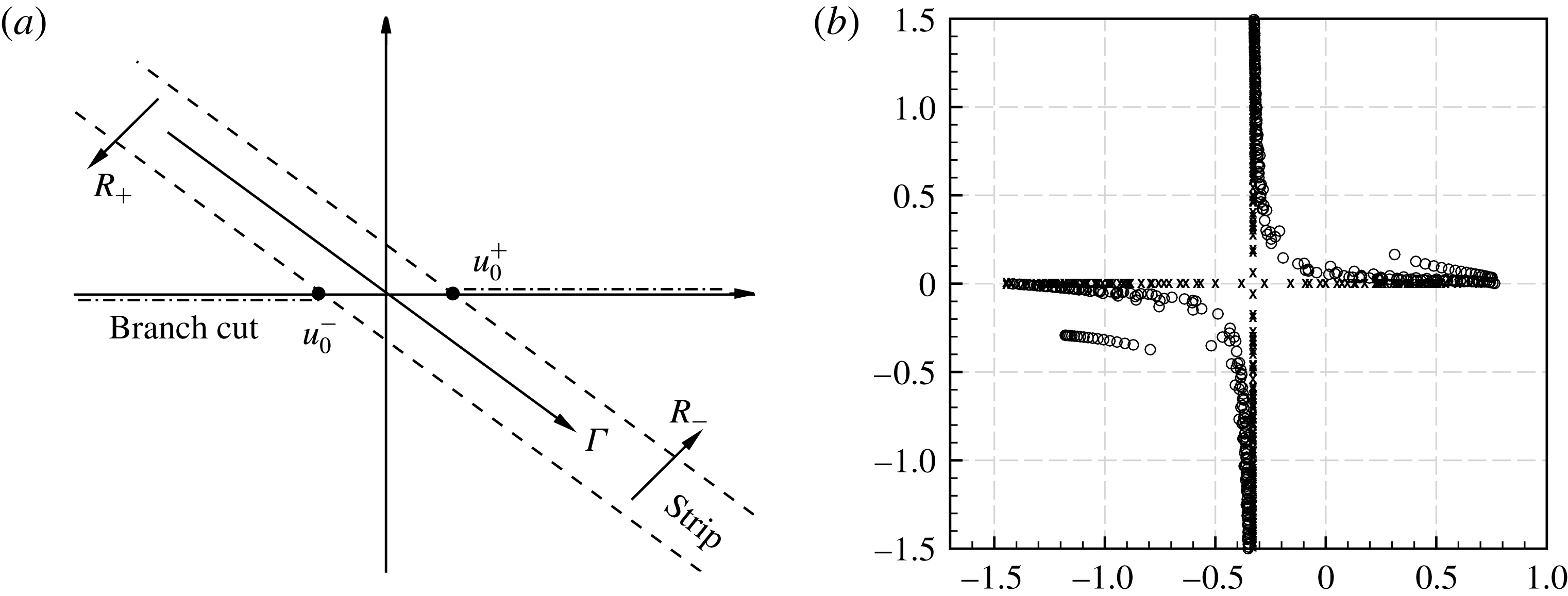
. The two branch cuts are two separate paths joining the branch points
 $u_{0}^{\pm }=1/(M\pm 1)$
to
 $\pm \infty$
through the two half-planes
 $R_{\mp }$
as shown in figure 3(a), respectively, where
 $R_{\pm }$
are defined as:
 $\pm \text{Im}(u-u_{0}^{\pm })<\mp \text{tan}(\unicode[STIX]{x1D716})\text{Re}(u-u_{0}^{\pm })$
, with
 $\unicode[STIX]{x1D716}=\text{tan}^{-1}(\text{Im}(\unicode[STIX]{x1D714})/\text{Re}(\unicode[STIX]{x1D714}))$
. The intersection of the two half-planes is a strip
 ${\mathcal{S}}$
. The solutions of (2.11) should have the form:
 $$\begin{eqnarray}\unicode[STIX]{x1D6FD}^{\unicode[STIX]{x1D705}}(u,r)=A^{\unicode[STIX]{x1D705}}(u)\text{J}_{m+\unicode[STIX]{x1D705}}(\unicode[STIX]{x1D706}\unicode[STIX]{x1D714}r),\end{eqnarray}$$
where
 $\text{J}_{m+\unicode[STIX]{x1D705}}$
is the
 $(m+\unicode[STIX]{x1D705})$
th-order Bessel function of the first kind and
 $A^{\unicode[STIX]{x1D705}}$
is the associated amplitude. From (2.12), The scattered field might consist of a series of circumferential modes other than the original mode
 $m$
of the incident wave, due to non-uniform impedance in the
 $\unicode[STIX]{x1D703}$
-direction.
(a) Schematic of the two complex half-planes
 $R_{\pm }$
and the overlapped strip when
 $M=0.3$
. The path of integration should be carefully designed to avoid all possible acoustic zeros and poles. (b) Poles (
 $\times$
) and zeros (○) of the matrix kernel
 $\mathscr{K}$
. The definition of poles and zeros of a matrix kernel can be found in our recent work (Huang Reference Huang2017). Incident wave with
 $\unicode[STIX]{x1D714}=25$
, mode
 $(18,1)$
,
 $M=0.3$
. The corresponding azimuthally non-uniform impedance distribution satisfies (4.1) that is to be defined in the following section, with
 $Z_{\unicode[STIX]{x1D6FC}}=1+0.5\text{i},Z_{\unicode[STIX]{x1D6FD}}=2-\text{i}$
and
 $N=1$
.

Similarly, we expand the Fourier transform of the vortex sheets into
 $$\begin{eqnarray}F_{+}(u,\unicode[STIX]{x1D703})=\int _{0}^{+\infty }\unicode[STIX]{x1D709}(x,\unicode[STIX]{x1D703})\text{e}^{-\text{i}\unicode[STIX]{x1D714}ux}\,\text{d}x=\mathop{\sum }_{\unicode[STIX]{x1D705}=-\infty }^{\infty }F_{+}^{\unicode[STIX]{x1D705}}(u)\text{e}^{\text{i}\unicode[STIX]{x1D705}\unicode[STIX]{x1D703}}.\end{eqnarray}$$
By first applying Fourier transform to (2.6) and then making use of (2.12)–(2.13), we will have the following relation:
 $A^{\unicode[STIX]{x1D705}}(u)=-\text{i}(1-uM)F_{+}^{\unicode[STIX]{x1D705}}(u)/\unicode[STIX]{x1D706}\text{J}_{m+\unicode[STIX]{x1D705}}^{\prime }(\unicode[STIX]{x1D706}\unicode[STIX]{x1D714})$
. Here
 $(\cdot )_{\pm }$
denotes the regularity in the half-planes
 $R_{\pm }$
, respectively, and all the functions
 $(\cdot )_{\pm }$
are regular in the overlapped strip
 ${\mathcal{S}}$
.
Then, we make one of the most important definitions as follows:
 $$\begin{eqnarray}\displaystyle & & \displaystyle \!\!G(u,\unicode[STIX]{x1D703})\triangleq \underbrace{\int _{0}^{+\infty }-\text{i}\unicode[STIX]{x1D714}\unicode[STIX]{x1D713}(x,\unicode[STIX]{x1D709}^{+},\unicode[STIX]{x1D703})\text{e}^{-\text{i}\unicode[STIX]{x1D714}ux}\,\text{d}x}_{\text{I}}\underbrace{-\int _{0}^{+\infty }\left(-\text{i}\unicode[STIX]{x1D714}+M\frac{\unicode[STIX]{x2202}}{\unicode[STIX]{x2202}x}\right)\unicode[STIX]{x1D713}_{s}(x,\unicode[STIX]{x1D709}^{-},\unicode[STIX]{x1D703})\text{e}^{-\text{i}\unicode[STIX]{x1D714}ux}\,\text{d}x}_{\text{II}}\nonumber\\ \displaystyle & & \displaystyle \quad \underbrace{-\int _{-\infty }^{0}\left(-\text{i}\unicode[STIX]{x1D714}+M\frac{\unicode[STIX]{x2202}}{\unicode[STIX]{x2202}x}\right)\unicode[STIX]{x1D713}_{s}(x,\unicode[STIX]{x1D709}^{-},\unicode[STIX]{x1D703})\text{e}^{-\text{i}\unicode[STIX]{x1D714}ux}\,\text{d}x}_{\text{III}},\end{eqnarray}$$
where
 $$\begin{eqnarray}\text{Term}\;\text{I}=\int _{0}^{+\infty }-p(x,\unicode[STIX]{x1D709}^{+},\unicode[STIX]{x1D703})\text{e}^{-\text{i}\unicode[STIX]{x1D714}ux}\,\text{d}x=\int _{0}^{+\infty }\text{i}\unicode[STIX]{x1D714}\unicode[STIX]{x1D709}(x,\unicode[STIX]{x1D703})Z(\unicode[STIX]{x1D714},\unicode[STIX]{x1D703})\text{e}^{-\text{i}\unicode[STIX]{x1D714}ux}\,\text{d}x,\end{eqnarray}$$
where
 $Z(\unicode[STIX]{x1D714},\unicode[STIX]{x1D703})$
is
 $2\unicode[STIX]{x03C0}$
-periodic in the
 $\unicode[STIX]{x1D703}$
-direction and, therefore, can be expanded into
 $$\begin{eqnarray}Z(\unicode[STIX]{x1D714},\unicode[STIX]{x1D703})=\mathop{\sum }_{\unicode[STIX]{x1D705}=-\infty }^{+\infty }Z^{\unicode[STIX]{x1D705}}(\unicode[STIX]{x1D714})\text{e}^{\text{i}\unicode[STIX]{x1D705}\unicode[STIX]{x1D703}},\quad Z^{\unicode[STIX]{x1D705}}(\unicode[STIX]{x1D714})=\frac{1}{2\unicode[STIX]{x03C0}}\int _{0}^{2\unicode[STIX]{x03C0}}Z(\unicode[STIX]{x1D714},\unicode[STIX]{x1D703})\text{e}^{-\text{i}\unicode[STIX]{x1D705}\unicode[STIX]{x1D703}}\,\text{d}\unicode[STIX]{x1D703},\end{eqnarray}$$
which leads Term I to
 $$\begin{eqnarray}\text{Term}\;\text{I}=\text{i}\unicode[STIX]{x1D714}\mathop{\sum }_{\unicode[STIX]{x1D705}=-\infty }^{+\infty }\mathop{\sum }_{\unicode[STIX]{x1D705}_{1}=-\infty }^{+\infty }Z^{\unicode[STIX]{x1D705}_{1}}(\unicode[STIX]{x1D714})F_{+}^{\unicode[STIX]{x1D705}-\unicode[STIX]{x1D705}_{1}}(u)\text{e}^{\text{i}\unicode[STIX]{x1D705}\unicode[STIX]{x1D703}}.\end{eqnarray}$$
Making use of (2.12), we also have
 $$\begin{eqnarray}\text{Terms}\;\text{II}+\text{III}=\mathop{\sum }_{\unicode[STIX]{x1D705}=-\infty }^{+\infty }\frac{\unicode[STIX]{x1D714}(1-uM)^{2}}{\unicode[STIX]{x1D706}}\frac{\text{J}_{m+\unicode[STIX]{x1D705}}(\unicode[STIX]{x1D706}\unicode[STIX]{x1D714})}{\text{J}_{m+\unicode[STIX]{x1D705}}^{\prime }(\unicode[STIX]{x1D706}\unicode[STIX]{x1D714})}F_{+}^{\unicode[STIX]{x1D705}}\text{e}^{\text{i}\unicode[STIX]{x1D705}\unicode[STIX]{x1D703}}.\end{eqnarray}$$
We can further define
 $G_{+}(u,\unicode[STIX]{x1D703})=\text{Terms I + II}$
and derive its analytical expression,
 $$\begin{eqnarray}\displaystyle G_{+}(u,\unicode[STIX]{x1D703})=\int _{0}^{+\infty }\left(-\text{i}\unicode[STIX]{x1D714}+M\frac{\unicode[STIX]{x2202}}{\unicode[STIX]{x2202}x}\right)\unicode[STIX]{x1D713}_{i}(\unicode[STIX]{x1D709}^{-})\text{e}^{-\text{i}\unicode[STIX]{x1D714}ux}\,\text{d}x=\frac{1-\unicode[STIX]{x1D707}_{mn}^{+}M}{\unicode[STIX]{x1D707}_{mn}^{+}-u}\text{J}_{m}(\unicode[STIX]{x1D6FC}_{mn}), & & \displaystyle\end{eqnarray}$$
which is obtained by using (2.7) along with (2.3), and the approximation
 $\unicode[STIX]{x1D709}^{-}\simeq 1$
. Meanwhile, we define
 $G_{-}(u,\unicode[STIX]{x1D703})\triangleq \text{Term}\;\text{III}=\sum _{\unicode[STIX]{x1D705}}G_{-}^{\unicode[STIX]{x1D705}}(u)\text{e}^{\text{i}\unicode[STIX]{x1D705}\unicode[STIX]{x1D703}}$
. Throughout this paper,
 $(\cdot )_{\pm }$
represents analytic functions in the upper and lower half-planes
 $R_{\mp }$
(as defined before (2.12)), respectively. Finally, by combining (2.17)–(2.19), we obtain the Wiener–Hopf equation:
 $$\begin{eqnarray}G_{+}+G_{-}=\text{i}\unicode[STIX]{x1D714}\mathop{\sum }_{\unicode[STIX]{x1D705}=-\infty }^{+\infty }\left(\mathop{\sum }_{\unicode[STIX]{x1D705}_{1}=-\infty }^{+\infty }Z^{\unicode[STIX]{x1D705}_{1}}(\unicode[STIX]{x1D714})F_{+}^{\unicode[STIX]{x1D705}-\unicode[STIX]{x1D705}_{1}}-\text{i}\frac{(1-uM)^{2}}{\unicode[STIX]{x1D706}}\frac{\text{J}_{m+\unicode[STIX]{x1D705}}(\unicode[STIX]{x1D706}\unicode[STIX]{x1D714})}{\text{J}_{m+\unicode[STIX]{x1D705}}^{\prime }(\unicode[STIX]{x1D706}\unicode[STIX]{x1D714})}F_{+}^{\unicode[STIX]{x1D705}}\right)\text{e}^{\text{i}\unicode[STIX]{x1D705}\unicode[STIX]{x1D703}},\end{eqnarray}$$
which leads to a matrix Wiener–Hopf model by equating the terms with the same
 $\text{exp}(\text{i}\unicode[STIX]{x1D705}\unicode[STIX]{x1D703})$
:
 $$\begin{eqnarray}\mathscr{K}\unicode[STIX]{x1D641}_{+}(u)=(\unicode[STIX]{x1D646}+\unicode[STIX]{x1D63E})\unicode[STIX]{x1D641}_{+}(u)=\unicode[STIX]{x1D642}_{-}(u)+\unicode[STIX]{x1D642}_{+}(u),\end{eqnarray}$$
with
 $$\begin{eqnarray}\displaystyle \left.\begin{array}{@{}c@{}}\unicode[STIX]{x1D646}=\left(\begin{array}{@{}ccccc@{}}\ddots & & & & \\ & K^{-1} & & & \\ & & K^{0} & & \\ & & & K^{1} & \\ & & & & \ddots \\ \end{array}\right);\quad \unicode[STIX]{x1D63E}=\text{i}\unicode[STIX]{x1D714}\left(\begin{array}{@{}ccccc@{}}\ddots & & & & \\ \cdots \, & 0 & Z^{-1} & Z^{-2} & \cdots \\ \cdots \, & Z^{1} & 0 & Z^{-1} & \cdots \\ \cdots \, & Z^{2} & Z^{1} & 0 & \cdots \\ & & & & \ddots \\ \end{array}\right);\\ \unicode[STIX]{x1D641}=\left(\begin{array}{@{}c@{}}\vdots \\ F_{+}^{-1}\\ F_{+}^{0}\\ F_{+}^{1}\\ \vdots \\ \end{array}\right);\quad \unicode[STIX]{x1D642}_{-}=\left(\begin{array}{@{}c@{}}\vdots \\ G_{-}^{-1}\\ G_{-}^{0}\\ G_{-}^{1}\\ \vdots \\ \end{array}\right);\quad \unicode[STIX]{x1D642}_{+}=\left(\begin{array}{@{}c@{}}\vdots \\ G_{+}^{-1}\\ G_{+}^{0}\\ G_{+}^{1}\\ \vdots \\ \end{array}\right).\end{array}\right\}\quad & & \displaystyle\end{eqnarray}$$
Here the constant matrix
 $\unicode[STIX]{x1D63E}$
is dependent on
 $Z(\unicode[STIX]{x1D714},\unicode[STIX]{x1D703})$
, and
 $\unicode[STIX]{x1D646}$
has the diagonal entries:
 $$\begin{eqnarray}K^{\unicode[STIX]{x1D705}}(u)=\unicode[STIX]{x1D714}(1-uM)^{2}\frac{\text{J}_{m+\unicode[STIX]{x1D705}}(\unicode[STIX]{x1D706}\unicode[STIX]{x1D714})}{\text{J}_{m+\unicode[STIX]{x1D705}}^{\prime }(\unicode[STIX]{x1D706}\unicode[STIX]{x1D714})}+\text{i}\unicode[STIX]{x1D714}Z^{0}(\unicode[STIX]{x1D714}).\end{eqnarray}$$
Physically, the poles and zeros (see figure 3
b) of each
 $K^{\unicode[STIX]{x1D705}}(u)$
correspond to the acoustic modes. The group of zeros of the determinant, det
 $\mathscr{K}$
(see (2.21)), is related to the dynamic behaviour of the vortex sheet. The equation of
 $K^{\unicode[STIX]{x1D705}}=0$
corresponds to the dispersion relation for uniformly lined ducts with a single azimuthal mode
 $m+\unicode[STIX]{x1D705}$
, while the matrix
 $\unicode[STIX]{x1D63E}$
represents the coupling between different azimuthal scattering waves excited by non-uniform impedance. It can be seen that (2.21) contains two unknowns,
 $\unicode[STIX]{x1D641}_{+}(u)$
and
 $\unicode[STIX]{x1D642}_{-}(u)$
. Hence, we utilise the analytic properties and apply the Wiener–Hopf method to solve this equation in the next section. A useful property for the application of the Wiener–Hopf method is the behaviour of the Wiener–Hopf kernel when
 $|u|\rightarrow \infty$
. Similar to Gabard & Astley (Reference Gabard and Astley2006), we find
 $\mathscr{K}\sim O(u^{2})$
as
 $|u|\rightarrow \infty$
in the strip
 ${\mathcal{S}}$
(as defined before (2.12)).
3 The revised Wiener–Hopf solution
The most essential (and usually difficult) step in the Wiener–Hopf method is the kernel factorisation. For the current matrix kernel
 $\mathscr{K}$
, we use the pole-removal method (Rawlins Reference Rawlins1980; Abrahams Reference Abrahams1987; Veitch & Peake Reference Veitch and Peake2008) to conduct the matrix factorisation. First, we directly factorise the diagonal matrix as:
 $\unicode[STIX]{x1D646}=\unicode[STIX]{x1D646}_{-}^{-1}\unicode[STIX]{x1D646}_{+}$
, where
 $\unicode[STIX]{x1D646}_{+}$
and
 $\unicode[STIX]{x1D646}_{-}$
are analytic, invertible and show algebraic behaviours at
 $\pm \infty$
. Then, from (2.21), we have:
 $$\begin{eqnarray}\displaystyle \unicode[STIX]{x1D646}_{+}(u)\unicode[STIX]{x1D641}_{+}(u)-\unicode[STIX]{x1D646}_{-}(\unicode[STIX]{x1D707}_{mn}^{+})\unicode[STIX]{x1D642}_{+}(u) & = & \displaystyle [\unicode[STIX]{x1D646}_{-}(u)-\unicode[STIX]{x1D646}_{-}(\unicode[STIX]{x1D707}_{mn}^{+})]\unicode[STIX]{x1D642}_{+}(u)\nonumber\\ \displaystyle & & \displaystyle +\,\unicode[STIX]{x1D646}_{-}(u)\unicode[STIX]{x1D642}_{-}(u)-\unicode[STIX]{x1D646}_{-}(u)\unicode[STIX]{x1D63E}\unicode[STIX]{x1D641}_{+}(u).\end{eqnarray}$$
The left-hand side of (3.1) is regular and non-zero in the plane
 $R_{+}$
(as defined before, see (2.12)). The subtraction of
 $\unicode[STIX]{x1D646}_{-}(\unicode[STIX]{x1D707}_{mn}^{+})\unicode[STIX]{x1D642}_{+}(u)$
on both sides of (3.1) cancels the pole
 $\unicode[STIX]{x1D707}_{mn}^{+}$
of
 $\unicode[STIX]{x1D642}_{+}(u)$
. Nevertheless, the right-hand side of (3.1) is still not regular in
 $R_{-}$
due to
 $\unicode[STIX]{x1D646}_{-}(u)\unicode[STIX]{x1D63E}\unicode[STIX]{x1D641}_{+}(u)$
. However, we can infer the singularity property of
 $\unicode[STIX]{x1D641}_{+}(u)$
in
 $R_{-}$
by studying
 $\mathscr{K}_{+}^{-1}=\mathscr{K}^{-1}\mathscr{K}_{-}^{-1}$
, where
 $\mathscr{K}_{-}^{-1}$
is analytic and invertible in
 $R_{-}$
. Then, apart from
 $\unicode[STIX]{x1D707}_{mn}^{+}$
, all singularities of
 $\unicode[STIX]{x1D641}_{+}(u)$
in
 $R_{-}$
are the same as the singularities of
 $\mathscr{K}^{-1}$
in
 $R_{-}$
(the detailed derivations can be found in appendix A). In addition,
 $\unicode[STIX]{x1D641}_{+}(u)$
only consists of meromorphic functions with a number of simple poles (denoted by
 $\unicode[STIX]{x1D6FD}_{j}^{-}$
with order
 $s_{j}$
,
 $j=0,1,2,\ldots$
), which are either poles of
 $\mathscr{K}$
(as shown in figure 3(b) with circular symbols in
 $R_{-}$
) or solutions of det
 $\mathscr{K}=0$
(since
 $\mathscr{K}^{-1}=\text{adj}\,\mathscr{K}/\text{det}\,\mathscr{K}$
, where
 $\text{adj}$
denotes the associated adjugate). Then, we first cancel the effect of the singularity
 $u=\unicode[STIX]{x1D707}_{mn}^{+}$
by introducing a term to both sides of (3.1) as follows:
 $$\begin{eqnarray}\displaystyle & & \displaystyle \unicode[STIX]{x1D646}_{+}(u)\unicode[STIX]{x1D641}_{+}(u)-\unicode[STIX]{x1D646}_{-}(\unicode[STIX]{x1D707}_{mn}^{+})\unicode[STIX]{x1D642}_{+}(u)+\unicode[STIX]{x1D646}_{-}(\unicode[STIX]{x1D707}_{mn}^{+})\unicode[STIX]{x1D63E}\unicode[STIX]{x1D641}_{+}(u)\nonumber\\ \displaystyle & & \displaystyle \quad =[\unicode[STIX]{x1D646}_{-}(u)-\unicode[STIX]{x1D646}_{-}(\unicode[STIX]{x1D707}_{mn}^{+})]\unicode[STIX]{x1D642}_{+}(u)+\unicode[STIX]{x1D646}_{-}(u)\unicode[STIX]{x1D642}_{-}(u)-[\unicode[STIX]{x1D646}_{-}(u)-\unicode[STIX]{x1D646}_{-}(\unicode[STIX]{x1D707}_{mn}^{+})]\unicode[STIX]{x1D63E}\unicode[STIX]{x1D641}_{+}(u).\quad\end{eqnarray}$$
Next, we apply the general pole-removal method to cancel the remaining poles,
 $\unicode[STIX]{x1D6FD}_{j}^{-}$
, of
 $\unicode[STIX]{x1D641}_{+}(u)$
in the half-plane
 $R_{-}$
,
 $$\begin{eqnarray}\displaystyle & & \displaystyle \unicode[STIX]{x1D646}_{+}(u)\unicode[STIX]{x1D641}_{+}(u)-\unicode[STIX]{x1D646}_{-}(\unicode[STIX]{x1D707}_{mn}^{+})[\unicode[STIX]{x1D642}_{+}(u)-\unicode[STIX]{x1D63E}\unicode[STIX]{x1D641}_{+}(u)]+\mathop{\sum }_{j=0}^{\infty }\frac{\mathscr{R}_{j}^{-}}{u-\unicode[STIX]{x1D6FD}_{j}^{-}}\nonumber\\ \displaystyle & & \displaystyle \quad =[\unicode[STIX]{x1D646}_{-}(u)-\unicode[STIX]{x1D646}_{-}(\unicode[STIX]{x1D707}_{mn}^{+})][\unicode[STIX]{x1D642}_{+}(u)-\unicode[STIX]{x1D63E}\unicode[STIX]{x1D641}_{+}(u)]+\unicode[STIX]{x1D646}_{-}(u)\unicode[STIX]{x1D642}_{-}(u)+\mathop{\sum }_{j=0}^{\infty }\frac{\mathscr{R}_{j}^{-}}{u-\unicode[STIX]{x1D6FD}_{j}^{-}},\end{eqnarray}$$
where
 $\mathscr{R}_{j}^{-}$
is a constant matrix, each element of which is the residue of the corresponding element in
 $[\unicode[STIX]{x1D646}_{-}(u)-\unicode[STIX]{x1D646}_{-}(\unicode[STIX]{x1D707}_{mn}^{+})]\unicode[STIX]{x1D63E}\unicode[STIX]{x1D641}_{+}(u)$
at the pole
 $u=\unicode[STIX]{x1D6FD}_{j}^{-}$
. Now both sides of (3.3) are analytic in the corresponding half-planes. By applying analytic continuation in complex analysis, (3.3) defines an entire function
 $\unicode[STIX]{x1D640}(u)$
that is regular in the whole complex
 $u$
plane. It is also easy to see that
 $\unicode[STIX]{x1D646}(u)\sim O(u^{2})$
and
 $\unicode[STIX]{x1D646}_{\pm }(u)\sim O(u^{\pm 1})$
as
 $|u|\rightarrow \infty$
. For outlet cases with
 $M>0$
, the full Kutta condition (Gabard & Astley Reference Gabard and Astley2006) should be adopted, so
 $\unicode[STIX]{x1D641}_{+}(u)\sim O(u^{-5/2})$
,
 $\unicode[STIX]{x1D642}_{-}(u)\sim O(u^{-1})$
; while for inlet cases with
 $M<0$
, we adopt the leading edge condition, resulting in
 $\unicode[STIX]{x1D641}_{+}(u)\sim O(u^{-3/2})$
. Therefore, we can obtain the entire function
 $\unicode[STIX]{x1D640}(u)\equiv 0$
for (3.3) as
 $u\rightarrow \infty$
. Here we wish to mention that it is possible to have a non-zero entire function if a different Kutta condition is adopted (Rienstra Reference Rienstra2007). However, the current governing equation is linear wave equation, and the unmodelled physics, such as nonlinearity and viscosity, should lead to a smooth behaviour of the edge condition that results in
 $\unicode[STIX]{x1D640}=0$
. A similar discussion can be found in Rienstra (Reference Rienstra2007)(before (32) therein). As a result,
 $$\begin{eqnarray}\unicode[STIX]{x1D641}_{+}(u)=[\unicode[STIX]{x1D646}_{+}(u)+\unicode[STIX]{x1D646}_{-}(\unicode[STIX]{x1D707}_{mn}^{+})\unicode[STIX]{x1D63E}]^{-1}\left[\unicode[STIX]{x1D646}_{-}(\unicode[STIX]{x1D707}_{mn}^{+})\unicode[STIX]{x1D642}_{+}(u)-\mathop{\sum }_{j=0}^{\infty }\frac{\mathscr{R}_{j}^{-}}{u-\unicode[STIX]{x1D6FD}_{j}^{-}}\right],\end{eqnarray}$$
where the infinitely many unknown residues,
 $\mathscr{R}_{j}^{-}$
, can be obtained by the approach proposed in the following (3.7). Finally, the solution of the total sound pressure fields is:
 $$\begin{eqnarray}p(x,r,\unicode[STIX]{x1D703})=p_{i}+\frac{\unicode[STIX]{x1D714}^{2}}{2\unicode[STIX]{x03C0}}\int _{\unicode[STIX]{x1D6E4}}\mathop{\sum }_{\unicode[STIX]{x1D705}=-\infty }^{+\infty }\frac{(1-uM)^{2}}{\unicode[STIX]{x1D706}}\frac{\text{J}_{m+\unicode[STIX]{x1D705}}(\unicode[STIX]{x1D706}\unicode[STIX]{x1D714}r)}{\text{J}_{m+\unicode[STIX]{x1D705}}^{\prime }(\unicode[STIX]{x1D706}\unicode[STIX]{x1D714})}F_{+}^{\unicode[STIX]{x1D705}}(u)\text{e}^{\text{i}(m+\unicode[STIX]{x1D705})\unicode[STIX]{x1D703}}\text{e}^{\text{i}\unicode[STIX]{x1D714}ux}\,\text{d}u,\end{eqnarray}$$
where the integral path
 $\unicode[STIX]{x1D6E4}$
is a curve from
 $-\infty \text{e}^{-\text{i}\unicode[STIX]{x1D716}}$
to
 $+\infty \text{e}^{-\text{i}\unicode[STIX]{x1D716}}$
in the strip
 ${\mathcal{S}}$
(Gabard & Astley Reference Gabard and Astley2006).
To enable the above pole removal in (3.3), we need to know the values of the residue. To this end, the values are still unknown. Here we propose an effective and interesting algorithm to obtain these values approximately. First, we rewrite (3.1) to
 $$\begin{eqnarray}\displaystyle & & \displaystyle \unicode[STIX]{x1D646}_{+}(u)\unicode[STIX]{x1D641}_{+}(u)-\unicode[STIX]{x1D646}_{-}(\unicode[STIX]{x1D707}_{mn}^{+})\unicode[STIX]{x1D642}_{+}(u)+\unicode[STIX]{x1D646}_{-}(u)\unicode[STIX]{x1D63E}\unicode[STIX]{x1D641}_{+}(u)\nonumber\\ \displaystyle & & \displaystyle \quad =[\unicode[STIX]{x1D646}_{-}(u)-\unicode[STIX]{x1D646}_{-}(\unicode[STIX]{x1D707}_{mn}^{+})]\unicode[STIX]{x1D642}_{+}(u)+\unicode[STIX]{x1D646}_{-}(u)\unicode[STIX]{x1D642}_{-}(u),\end{eqnarray}$$
where
 $\unicode[STIX]{x1D646}_{-}(\unicode[STIX]{x1D707}_{mn}^{+})\unicode[STIX]{x1D642}_{+}(u)$
on both sides of (3.6) cancels the pole
 $\unicode[STIX]{x1D707}_{mn}^{+}$
of
 $\unicode[STIX]{x1D642}_{+}(u)$
. However, the left-hand side of (3.6) is still not regular in
 $R_{+}$
due to
 $\unicode[STIX]{x1D646}_{-}(u)$
with poles in
 $R_{+}$
(these poles in
 $R_{+}$
are denoted by
 $\unicode[STIX]{x1D6FD}_{j}^{+},j=0,1,2,\ldots$
). By using the pole removal technique to further remove these poles from (3.6), we have
 $$\begin{eqnarray}\displaystyle & & \displaystyle \unicode[STIX]{x1D646}_{+}(u)\unicode[STIX]{x1D641}_{+}(u)-\unicode[STIX]{x1D646}_{-}(\unicode[STIX]{x1D707}_{mn}^{+})\unicode[STIX]{x1D642}_{+}(u)+\left[\unicode[STIX]{x1D646}_{-}(u)\unicode[STIX]{x1D63E}\unicode[STIX]{x1D641}_{+}(u)-\mathop{\sum }_{j=0}^{\infty }\frac{\mathscr{R}_{j}^{+}}{u-\unicode[STIX]{x1D6FD}_{j}^{+}}\right]\nonumber\\ \displaystyle & & \displaystyle \quad =[\unicode[STIX]{x1D646}_{-}(u)-\unicode[STIX]{x1D646}_{-}(\unicode[STIX]{x1D707}_{mn}^{+})]\unicode[STIX]{x1D642}_{+}(u)+\unicode[STIX]{x1D646}_{-}(u)\unicode[STIX]{x1D642}_{-}(u)-\mathop{\sum }_{j=0}^{\infty }\frac{\mathscr{R}_{j}^{+}}{u-\unicode[STIX]{x1D6FD}_{j}^{+}},\end{eqnarray}$$
where
 $\mathscr{R}_{j}^{+}$
is the residue for
 $\unicode[STIX]{x1D646}_{-}(u)\unicode[STIX]{x1D63E}\unicode[STIX]{x1D641}_{+}(u)$
at the corresponding pole
 $u=\unicode[STIX]{x1D6FD}_{j}^{+}$
in the upper half-plane. Now both sides of (3.7) are analytic in the corresponding half-planes. Once again, it is easy to obtain an entire function
 $\unicode[STIX]{x1D640}(u)\equiv 0$
for (3.7) as
 $u\rightarrow \infty$
, resulting in
 $$\begin{eqnarray}\unicode[STIX]{x1D641}_{+}(u)=[\unicode[STIX]{x1D646}_{+}(u)+\unicode[STIX]{x1D646}_{-}(u)\unicode[STIX]{x1D63E}]^{-1}\left[\unicode[STIX]{x1D646}_{-}(\unicode[STIX]{x1D707}_{mn}^{+})\unicode[STIX]{x1D642}_{+}(u)+\mathop{\sum }_{j=0}^{\infty }\frac{\mathscr{R}_{j}^{+}}{u-\unicode[STIX]{x1D6FD}_{j}^{+}}\right].\end{eqnarray}$$
We have two different solutions for
 $\unicode[STIX]{x1D641}_{+}(u)$
, i.e. (3.4) and (3.8), with many unknown residue values
 $\mathscr{R}_{j}^{\pm }$
,
 $j=0,1,\ldots .$
By carefully comparing (3.4) and (3.8), we find that from (3.4) we can calculate
 $\mathscr{R}_{j}^{+}$
, while from (3.8) we can calculate
 $\mathscr{R}_{j}^{-}$
, together these constitute a closed set of equations. For simplicity, we assume a problem set-up with only four residues,
 $\mathscr{R}_{0}^{\pm }$
and
 $\mathscr{R}_{1}^{\pm }$
. Then, the corresponding equations are
 $$\begin{eqnarray}\left.\begin{array}{@{}c@{}}\displaystyle \mathscr{R}_{1}^{+}=\boldsymbol{U}(\unicode[STIX]{x1D6FD}_{1}^{+})\left[\unicode[STIX]{x1D646}_{-}(\unicode[STIX]{x1D707}_{mn}^{+})\unicode[STIX]{x1D642}_{+}(\unicode[STIX]{x1D6FD}_{1}^{+})-\frac{\mathscr{R}_{0}^{-}}{\unicode[STIX]{x1D6FD}_{1}^{+}-\unicode[STIX]{x1D6FD}_{0}^{-}}-\frac{\mathscr{R}_{1}^{-}}{\unicode[STIX]{x1D6FD}_{1}^{+}-\unicode[STIX]{x1D6FD}_{1}^{-}}\right],\\ \displaystyle \mathscr{R}_{0}^{+}=\boldsymbol{U}(\unicode[STIX]{x1D6FD}_{0}^{+})\left[\unicode[STIX]{x1D646}_{-}(\unicode[STIX]{x1D707}_{mn}^{+})\unicode[STIX]{x1D642}_{+}(\unicode[STIX]{x1D6FD}_{0}^{+})-\frac{\mathscr{R}_{0}^{-}}{\unicode[STIX]{x1D6FD}_{0}^{+}-\unicode[STIX]{x1D6FD}_{0}^{-}}-\frac{\mathscr{R}_{1}^{-}}{\unicode[STIX]{x1D6FD}_{0}^{+}-\unicode[STIX]{x1D6FD}_{1}^{-}}\right],\\ \displaystyle \mathscr{R}_{0}^{-}=\boldsymbol{V}(\unicode[STIX]{x1D6FD}_{0}^{-})\left[\unicode[STIX]{x1D646}_{-}(\unicode[STIX]{x1D707}_{mn}^{+})\unicode[STIX]{x1D642}_{+}(\unicode[STIX]{x1D6FD}_{0}^{-})+\frac{\mathscr{R}_{0}^{+}}{\unicode[STIX]{x1D6FD}_{0}^{-}-\unicode[STIX]{x1D6FD}_{0}^{+}}+\frac{\mathscr{R}_{1}^{+}}{\unicode[STIX]{x1D6FD}_{0}^{-}-\unicode[STIX]{x1D6FD}_{1}^{+}}\right],\\ \displaystyle \mathscr{R}_{1}^{-}=\boldsymbol{V}(\unicode[STIX]{x1D6FD}_{1}^{-})\left[\unicode[STIX]{x1D646}_{-}(\unicode[STIX]{x1D707}_{mn}^{+})\unicode[STIX]{x1D642}_{+}(\unicode[STIX]{x1D6FD}_{1}^{-})+\frac{\mathscr{R}_{0}^{+}}{\unicode[STIX]{x1D6FD}_{1}^{-}-\unicode[STIX]{x1D6FD}_{0}^{+}}+\frac{\mathscr{R}_{1}^{+}}{\unicode[STIX]{x1D6FD}_{1}^{-}-\unicode[STIX]{x1D6FD}_{1}^{+}}\right],\end{array}\right\}\end{eqnarray}$$
where
 $$\begin{eqnarray}\displaystyle & \displaystyle \boldsymbol{U}(\mathfrak{z})=\underset{u\rightarrow \mathfrak{z}}{\text{Res}}[\unicode[STIX]{x1D646}_{-}(u)]\unicode[STIX]{x1D63E}[\unicode[STIX]{x1D646}_{+}(\mathfrak{z})+\unicode[STIX]{x1D646}_{-}(\unicode[STIX]{x1D707}_{mn}^{+})\unicode[STIX]{x1D63E}]^{-1}, & \displaystyle\end{eqnarray}$$
 $$\begin{eqnarray}\displaystyle & \displaystyle \boldsymbol{V}(\mathfrak{z})=[\unicode[STIX]{x1D646}_{-}(\mathfrak{z})-\unicode[STIX]{x1D646}_{-}(\unicode[STIX]{x1D707}_{mn}^{+})]\unicode[STIX]{x1D63E}\,\underset{u\rightarrow \mathfrak{z}}{\text{Res}}\{[\unicode[STIX]{x1D646}_{+}(u)+\unicode[STIX]{x1D646}_{-}(u)\unicode[STIX]{x1D63E}]^{-1}\}. & \displaystyle\end{eqnarray}$$
The above four equations are closed with four unknown residues
 $\mathscr{R}_{0,1}^{\pm }$
at
 $\unicode[STIX]{x1D6FD}_{0,1}^{\pm }$
. Of course, a practical problem set-up usually contains many poles and zeros and a truncation operation has to be adopted to enable a numerical implementation. Generally, for
 $2\mathscr{N}$
poles (
 $\unicode[STIX]{x1D6FD}_{j}^{\pm }$
,
 $j=0,1,\ldots ,\mathscr{N}-1$
), we can obtain the corresponding residue values by the following generic formulation:
 $$\begin{eqnarray}\mathscr{R}=\mathscr{A}^{-1}\mathscr{B},\end{eqnarray}$$
where
 $$\begin{eqnarray}\displaystyle \mathscr{A}=\left[\left(\begin{array}{@{}cc@{}}\boldsymbol{I} & \mathscr{C}\\ \mathscr{D} & \boldsymbol{I}\\ \end{array}\right)\right]_{2\mathscr{N}\times 2\mathscr{N}},\quad \mathscr{R}=[\ldots ,\mathscr{R}_{1}^{+},\mathscr{R}_{0}^{+},\mathscr{R}_{0}^{-},\mathscr{R}_{1}^{-},\ldots ]^{\text{T}}, & & \displaystyle\end{eqnarray}$$
 $$\begin{eqnarray}\displaystyle & \displaystyle \mathscr{C}_{ij}=\boldsymbol{U}(\unicode[STIX]{x1D6FD}_{\mathscr{N}-i}^{+})/(\unicode[STIX]{x1D6FD}_{\mathscr{N}-i}^{+}-\unicode[STIX]{x1D6FD}_{j-1}^{-}), & \displaystyle\end{eqnarray}$$
 $$\begin{eqnarray}\displaystyle & \displaystyle \mathscr{D}_{ij}=\boldsymbol{V}(\unicode[STIX]{x1D6FD}_{i-1}^{-})/(\unicode[STIX]{x1D6FD}_{\mathscr{N}-j}^{+}-\unicode[STIX]{x1D6FD}_{i-1}^{-}), & \displaystyle\end{eqnarray}$$
 $$\begin{eqnarray}\displaystyle & \displaystyle \mathscr{B}_{i}=\boldsymbol{U}(\unicode[STIX]{x1D6FD}_{\mathscr{N}-i}^{+})\unicode[STIX]{x1D646}_{-}(\unicode[STIX]{x1D707}_{mn}^{+})\unicode[STIX]{x1D642}_{+}(\unicode[STIX]{x1D6FD}_{\mathscr{N}-i}^{+}), & \displaystyle\end{eqnarray}$$
 $$\begin{eqnarray}\displaystyle & \displaystyle \mathscr{B}_{\mathscr{N}+i}=\boldsymbol{V}(\unicode[STIX]{x1D6FD}_{i-1}^{-})\unicode[STIX]{x1D646}_{-}(\unicode[STIX]{x1D707}_{mn}^{+})\unicode[STIX]{x1D642}_{+}(\unicode[STIX]{x1D6FD}_{i-1}^{-}), & \displaystyle\end{eqnarray}$$
 $$\begin{eqnarray}\displaystyle i=1,2,\ldots ,\mathscr{N},\quad j=1,2,\ldots ,\mathscr{N}. & & \displaystyle\end{eqnarray}$$
Physically, the
 $j=0$
pole corresponds to a modal element with the smallest mode number,
 $j=1$
corresponds to the second smallest mode number, and so on.
Given a problem set-up, we will first set an appropriate truncation number
 $\mathscr{N}$
and solve (3.12) to obtain the corresponding residue values. Then, we can use either (3.4) or (3.8) to solve
 $\unicode[STIX]{x1D641}_{+}(u)$
. Eventually, we solve (3.5) to produce the whole sound wave field. If
 $\mathscr{N}$
is set to 0, the effect due to those poles is neglected and the current model follows the same simplification strategy adopted in the previous work (Liu et al.
Reference Liu, Jiang, Huang and Chen2015).
4 Results and discussion
To demonstrate the proposed model, we prepare a couple of test cases. First, we verify the numerical implementation by examining a simple flow duct case with uniform, semi-infinite axial liners. The current model can exactly recover the same results of the previous model (Rienstra Reference Rienstra2007) because
 $\unicode[STIX]{x1D63E}=0$
in that case, meaning that there are no poles to remove. The corresponding results are omitted for brevity. Then, we consider azimuthally non-uniform liner cases with two representative impedance distributions: one has a segmental set-up with two different acoustic impedance values,
 $Z_{\unicode[STIX]{x1D6FC}}$
and
 $Z_{\unicode[STIX]{x1D6FD}}$
, resulting in the following distribution
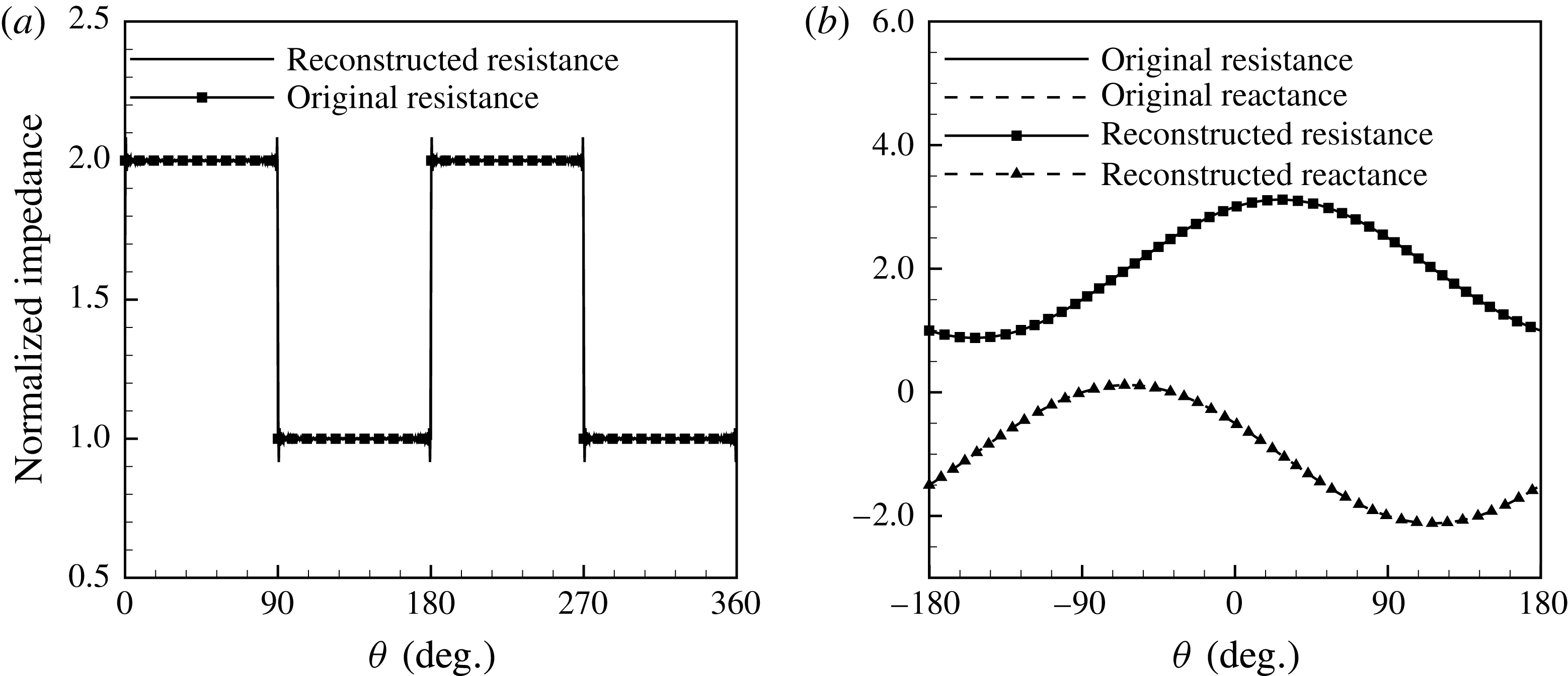
 $$\begin{eqnarray}\displaystyle Z(\unicode[STIX]{x1D703})=\left\{\begin{array}{@{}ll@{}}Z_{\unicode[STIX]{x1D6FC}},\quad & \text{if }(2j-2)\unicode[STIX]{x03C0}/N<\unicode[STIX]{x1D703}\leqslant (2j-1)\unicode[STIX]{x03C0}/N,\\ Z_{\unicode[STIX]{x1D6FD}},\quad & \text{if }(2j-1)\unicode[STIX]{x03C0}/N<\unicode[STIX]{x1D703}\leqslant 2j\unicode[STIX]{x03C0}/N,\end{array}\right. & & \displaystyle\end{eqnarray}$$
where
 $j=1,2,\ldots ,N$
with
 $N$
the number of segments; and the other has a sinusoidal distribution
 $$\begin{eqnarray}\displaystyle Z(\unicode[STIX]{x1D703})=Z_{\unicode[STIX]{x1D6FC}}\text{e}^{\text{i}N\unicode[STIX]{x1D703}}+Z_{\unicode[STIX]{x1D6FD}}, & & \displaystyle\end{eqnarray}$$
where
 $Z_{\unicode[STIX]{x1D6FC}}$
and
 $Z_{\unicode[STIX]{x1D6FD}}$
are two constant parameters to be defined by users. For example, figure 4 shows the associated azimuthal distributions under certain parameters.


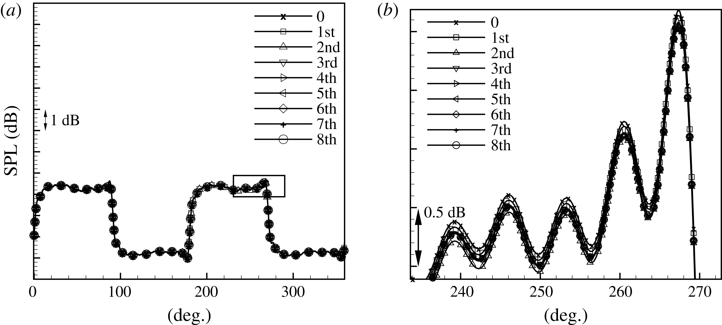
Study of the truncation issue, where (a) the sound pressure level (
 $\text{SPL}=20~\text{log}_{10}(p_{rms}/2\times 10^{-5})$
, with
 $(\cdot )_{rms}$
the root mean square value) results at
 $(x,r)=(0.1,1)$
, where
 $(m,n)=(24,1)$
, Mach number
 $M=0.3$
,
 $\unicode[STIX]{x1D714}=30$
and impedance
 $Z_{\unicode[STIX]{x1D6FC}}=1+1\text{i}$
,
 $Z_{\unicode[STIX]{x1D6FD}}=2+2\text{i}$
and
 $N=2$
. First, we set
 $\mathscr{N}=0$
and do not perform pole removal. Then, we gradually remove the associated 8 poles from
 $K^{0}$
. (b) An enlarged view shows that the pole-removal operation for the current set-up only introduces slight modifications.

First, we use the case set-up with an impedance distribution such as (4.1) to examine the truncation issue. Given a problem set-up (the spinning mode number
 $(m,n)=(24,1)$
, Mach number
 $M=0.3$
,
 $\unicode[STIX]{x1D714}=30$
and impedance
 $Z_{\unicode[STIX]{x1D6FC}}=1+1\text{i}$
,
 $Z_{\unicode[STIX]{x1D6FD}}=2+2\text{i}$
and
 $N=2$
). To check the convergence, we remove those poles one by one, by using either (3.4) or (3.8), and compare the corresponding solutions. The sound pressure results shown in figure 5 shows that the pole-removal technique introduces little difference to the final predictions. Here we only remove the poles of
 $K^{0}$
but the same observations have been found when we further remove the poles of
 $K^{\pm 2}$
. Overall, figure 5 suggests that the effect due to those poles from the matrix kernel is negligible. Therefore, the simplified strategy adopted in the previous work (Liu et al.
Reference Liu, Jiang, Huang and Chen2015) is acceptable, even for the current more generic case set-ups. As a result, we also apply the same strategy to study the set-ups with azimuthally non-uniform liner in this work.
The SPL results at
 $(x,r)=(0.1,1),(0.3,1)$
and
 $(0.5,1)$
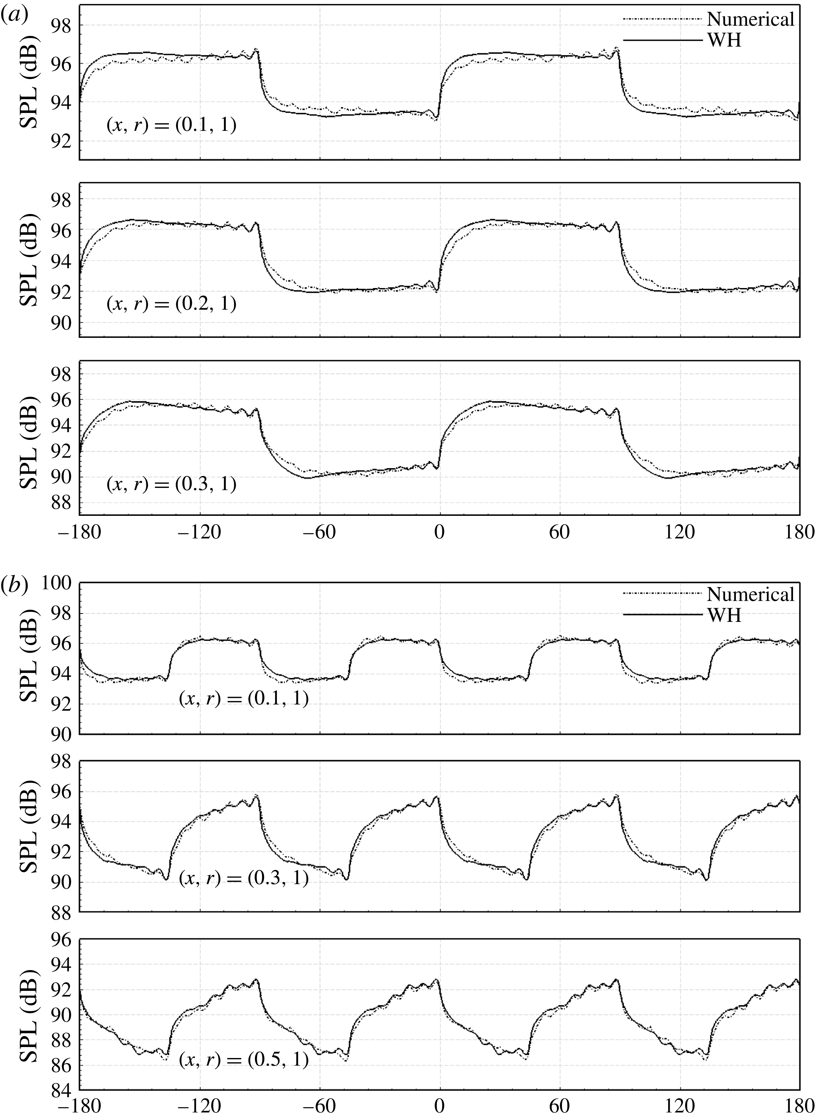
calculated by the proposed Wiener–Hopf analytical model and the numerical solver, respectively. The horizontal axis represents
 $\unicode[STIX]{x1D703}$
(deg.). The set-up is
 $(m,n)=(24,1)$
, Mach number
 $M=0.3$
,
 $\unicode[STIX]{x1D714}=30$
and impedance
 $Z_{\unicode[STIX]{x1D6FC}}=1+1\text{i}$
,
 $Z_{\unicode[STIX]{x1D6FD}}=2+2\text{i}$
, for (a)
 $N=2$
and (b)
 $N=4$
.

Instantaneous sound pressure field, with incident spinning mode
 $(18,1)$
,
 $\unicode[STIX]{x1D714}=25$
,
 $M=0.3$
,
 $N=-1$
and
 $Z$
is given by (4.2), where
 $Z_{\unicode[STIX]{x1D6FC}}=1+0.5\text{i}$
,
 $Z_{\unicode[STIX]{x1D6FD}}=2-1\text{i}$
.

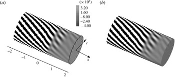
Instantaneous sound pressure field solved (a) by the proposed theoretical model and (b) by the commercial software ACTRAN®, where the incident spinning mode
 $(18,1)$
,
 $\unicode[STIX]{x1D714}=25$
,
 $M=0.3$
,
 $N=-1$
and
 $Z$
is given by (4.2), where
 $Z_{\unicode[STIX]{x1D6FC}}=1+0.5\text{i}$
,
 $Z_{\unicode[STIX]{x1D6FD}}=2-1\text{i}$
.

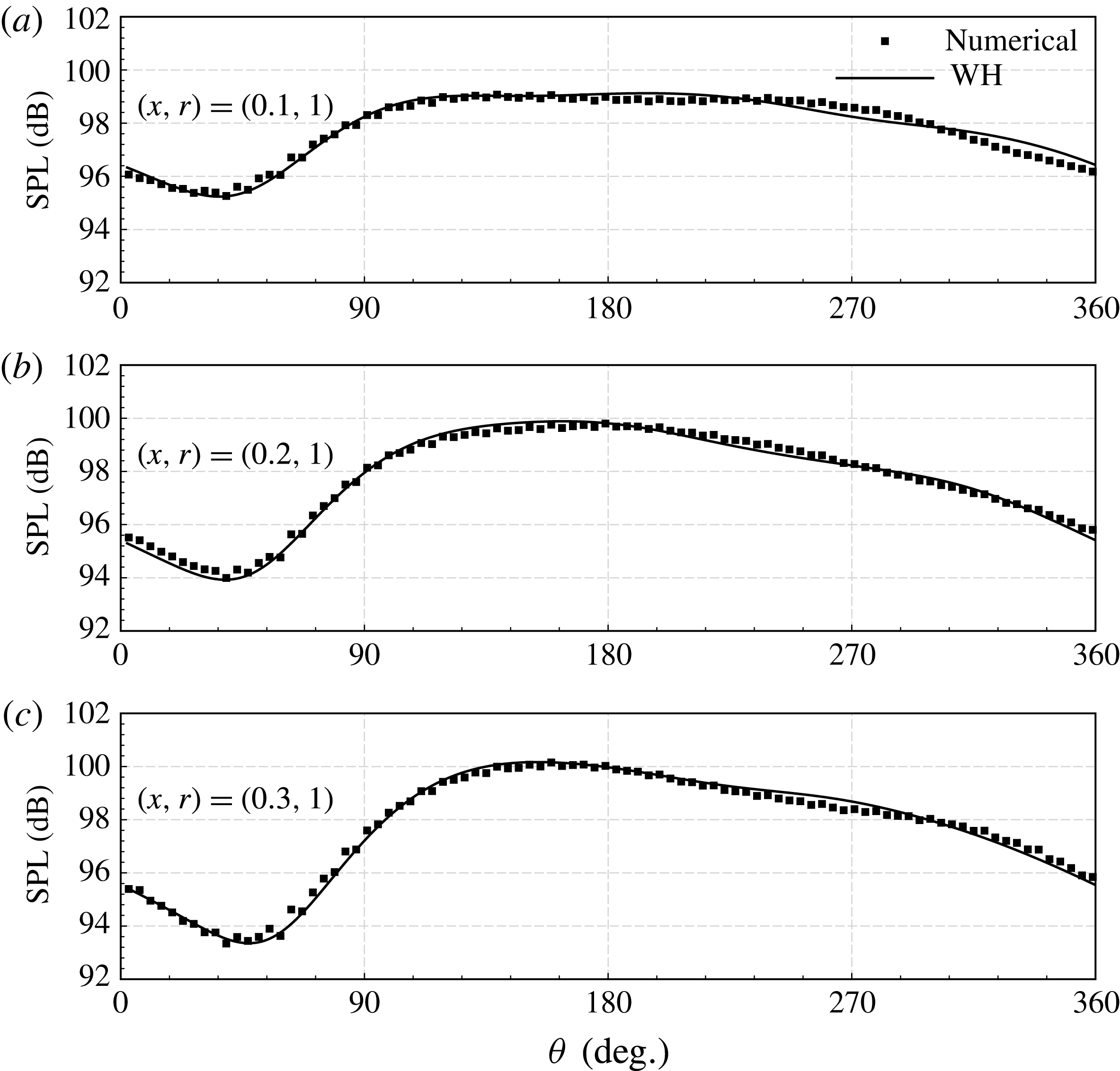
Figures 6 and 7 compare the model predictions to the numerical results from the commercial finite element software, ACTRAN®. Both the piecewise segmental impedance values, (4.1), and the sinusoidal impedance values, (4.2), are examined. It can be seen that the analytical and the numerical results agree very well in most regions, with the largest difference less than 0.5 dB. The wiggles of the sound pressure level (SPL) results around the different interfaces between two lined segments are well captured by the theoretical model. In addition, the SPL results along the duct wall (
 $r=1$
) share the same periodicity with the segments, which indicates that there exist new circumferential modes other than the modes of incident waves, and the new modes should be directly related to the parameter
 $N$
which is defined previously to represent the distribution of liner impedance
 $Z(\unicode[STIX]{x1D703})$
. Finally, figure 8 shows the overall surface sound pressure field for the azimuthally sinusoidal distribution. Once again, it can be seen that the agreement between the theoretical prediction and the computational result is very good.
Instantaneous sound pressure fields in the
 $(r,\unicode[STIX]{x1D703})$
cross-sections at
 $x=0.1,0.3$
and
 $0.5$
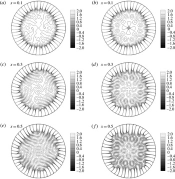
. (a,c,e) Show results for the piecewise segmental liner with (4.1). (b,d,f) Show results for the sinusoidal liner with (4.2). Other configurations are the same as figure 6(b) and figure 8, respectively.

Modal spectrum of instantaneous sound pressure field at
 $x=0.1$
are shown here with respect to circumferential and radial modes. The parameters are same as figure 6, besides (a)
 $N=2$
and (b)
 $N=4$
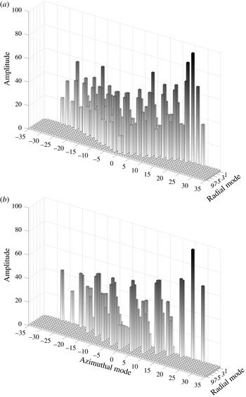
.

To investigate the effect of liner non-uniformity, we first calculate the modal spectrum (shown in figure 10) at
 $x=0.1$
cross-section for results shown in figure 9. For a set-up of dimensionless frequency
 $\unicode[STIX]{x1D714}=30$
and background flow
 $M=0.3$
, modes of circumferential order greater than 28 or less than
 $-$
28 are cutoff (the sign of
 $m$
denotes if the mode is spinning clockwise or counterclockwise). It can be seen that the single mode injected is scattered, yielding many new azimuthal modes. As is expected, the modal spectrum has gaps in azimuthal mode axis and the width of each gap is equal to
 $N$
, which is the number of periods of
 $Z(\unicode[STIX]{x1D703})$
in
 $2\unicode[STIX]{x03C0}$
. Furthermore, the patterns in figure 9 suggest that the single incident mode is scattered into many new azimuthal modes.
In this work, the proposed theoretical model is implemented with MATLAB®. The computational cost on a desktop computer with Intel® Core E5 processor @ 3.30 GHz is of the order of
 $O(10^{2})\;\text{s}$
. As a comparison, the same set-up is solved by a commercial numerical solver, ACTRAN®, on the same computer. Each three-dimensional unstructured mesh used in the calculation has
 $3\times 10^{6}$
grid points and the geometrical domain of
 $-2\leqslant x\leqslant 2$
,
 $0\leqslant r\leqslant 1$
and
 $0\leqslant \unicode[STIX]{x1D703}\leqslant 2\unicode[STIX]{x03C0}$
is considered. The computational cost is of the order of
 $O(10^{4})\;\text{s}$
, which is two orders of magnitude greater than that of the proposed model. Moreover, when a computational solver such as ACTRAN® is used for more complicated set-ups with more irregular and azimuthally non-uniform impedance values, the preparation of the computational meshes and other initial numerical settings will become even more tedious. In contrast, the proposed theoretical model can rapidly predict sound fields for various azimuthal distributions by a simple change of the corresponding mathematical formula. Therefore, the proposed model is more computationally efficient and convenient to use compared to three-dimensional numerical solvers.
Overall, figures 8 and 9 suggest two possible new noise control strategies by using azimuthally non-uniform liner designs. First, when the number of segments is much larger than the azimuthal mode of incident waves, it is possible to make all the scattered modes cutoff. As a result, each azimuthal segment can be designed to especially attenuate a particular incident wave at a certain frequency, which will enable a broadband liner design. Second, the azimuthal distribution can be carefully designed to re-direct sound propagation to certain angles and thus minimise the interference to other regions.
5 Summary
In this work, we have developed an analytical model for the modelling of flow duct liners with azimuthally non-uniform impedance. To enable the theoretical development, we have to assume an axial symmetrical duct enclosing uniform mean steady flow. By adopting some modifications, it may be possible to apply the proposed modelling method to a slightly curved duct with non-uniform steady flow. However, we believe the resultant model will become less (mathematically) delicate and a direct numerical simulation may be more appropriate for such practical set-ups.
For the current idealised set-up with straightened ducts, we have incorporated Fourier series expansion into the Wiener–Hopf method to investigate spinning modal sound wave scattering from the axial hard–soft interface and azimuthally non-uniform lined walls. The key achievement of this work is the development of the mathematical model and the interesting technique applied in the pole-removal process. In particular, two sets of Wiener–Hopf equations are organised to infer the residues in the upper and lower half-planes, which enable the subsequent matrix kernel factorisation. Another key observation is that the effect due to the removed poles are usually negligible, at least for the current segmental and sinusoidal impedance distributions in the azimuthal direction. As a result, we are also able to validate the simplified strategy adopted in matrix kernel factorisation in a previous work (Liu et al. Reference Liu, Jiang, Huang and Chen2015). Moreover, the proposed model has a distinctive feature that allows it to shed light on the associated physical mechanism of the scattering process, i.e. new modes directly depend on the azimuthal distribution will be scattered.
Although the rapid development of new materials makes it possible to design and employ liners with azimuthally non-uniform impedance inside engine duct to reduce noise emission more effectively, three-dimensional numerical solvers for non-uniform liners are usually computationally expensive for liner optimisation which often requires thousands of runs (Jiang et al. Reference Jiang, Lau and Huang2017b ). The efficiency of the proposed analytical model is at least two orders of magnitude higher than that of three-dimensional numerical solvers. Therefore, the current analytical model should be very useful for a host of new aeroengine (and even airframe (Boorsma, Zhang & Molin Reference Boorsma, Zhang and Molin2010)) liner design and optimisation problems.
Acknowledgements
This work is partly supported by National Science Foundation of China (Grant no. 11561130148 and 11772005). Lau received Post-Doctoral Fellowship Matching Fund from the Hong Kong University of Science and Technology. Huang received the Newton Advanced Fellowship from the Royal Society (Ref: NA14081).
Appendix A. The singularities of
$\unicode[STIX]{x1D641}_{+}(u)$
in
$R_{-}$


Suppose
 $\mathscr{K}$
in (2.21) can be factorised to:
 $\mathscr{K}_{+}(u)=\mathscr{K}_{-}(u)\mathscr{K}(u)$
, where
 $\mathscr{K}_{\pm }(u)$
are regular and non-zero in
 $R_{\pm }$
, respectively. Then, we have
 $$\begin{eqnarray}\mathscr{K}_{+}(u)\unicode[STIX]{x1D641}_{+}(u)=\mathscr{K}_{-}(u)\unicode[STIX]{x1D642}_{-}(u)+\mathscr{K}_{-}(u)\unicode[STIX]{x1D642}_{+}(u).\end{eqnarray}$$
According to (2.19),
 $\unicode[STIX]{x1D642}_{+}(u)$
is regular in the whole
 $u$
-plane except for the single pole
 $u=\unicode[STIX]{x1D707}_{mn}^{+}$
, which is cancelled by introducing an additional term,
 $-\mathscr{K}_{-}(\unicode[STIX]{x1D707}_{mn}^{+})\unicode[STIX]{x1D642}_{+}(u)$
, on both sides of (A 1):
 $$\begin{eqnarray}\mathscr{K}_{+}(u)\unicode[STIX]{x1D641}_{+}(u)-\mathscr{K}_{-}(\unicode[STIX]{x1D707}_{mn}^{+})\unicode[STIX]{x1D642}_{+}(u)=[\mathscr{K}_{-}(u)-\mathscr{K}_{-}(\unicode[STIX]{x1D707}_{mn}^{+})]\unicode[STIX]{x1D642}_{+}(u)+\mathscr{K}_{-}(u)\unicode[STIX]{x1D642}_{-}(u).\end{eqnarray}$$
To this end, both left- and right-hand sides of (A 2) are regular in
 $R_{+}$
and
 $R_{-}$
, respectively. Then, by analytic continuation, we can find an entire function
 $\unicode[STIX]{x1D640}(u)$
that is regular on the whole
 $u$
-plane and equal to both sides of (A 2). Next, it is easy to see that
 $\mathscr{K}(u)\sim O(u^{2})$
and
 $\mathscr{K}_{\pm }(u)\sim O(u^{\pm 1})$
as
 $|u|\rightarrow \infty$
(see appendix B). For outlet cases with
 $M>0$
, the full Kutta condition (Gabard & Astley Reference Gabard and Astley2006) should be adopted, so
 $\unicode[STIX]{x1D641}_{+}(u)\sim O(u^{-5/2})$
,
 $\unicode[STIX]{x1D642}_{-}(u)\sim O(u^{-1})$
, and
 $\mathscr{E}(u)\sim O(u^{-2})$
; while for inlet cases with
 $M<0$
, we adopt the leading edge condition, resulting in
 $\unicode[STIX]{x1D641}_{+}(u)\sim O(u^{-3/2}),\unicode[STIX]{x1D642}_{-}(u)\sim O(u^{-1/2})$
. Overall, we have
 $\unicode[STIX]{x1D640}(u)\equiv 0$
, as
 $|u|\rightarrow \infty$
. Therefore, we have:
 $$\begin{eqnarray}\unicode[STIX]{x1D641}_{+}(u)=\mathscr{K}_{+}^{-1}(u)\mathscr{K}_{-}(\unicode[STIX]{x1D707}_{mn}^{+})\unicode[STIX]{x1D642}_{+}(u)=\mathscr{K}^{-1}(u)\mathscr{K}_{-}^{-1}(u)\mathscr{K}_{-}(\unicode[STIX]{x1D707}_{mn}^{+})\unicode[STIX]{x1D642}_{+}(u).\end{eqnarray}$$
Then, we achieve the conclusion that all singularities of
 $\unicode[STIX]{x1D641}_{+}(u)$
in
 $R_{-}$
are the same as the singularities of
 $\mathscr{K}^{-1}$
in
 $R_{-}$
plus the additional singularity
 $u=\unicode[STIX]{x1D707}_{mn}^{+}$
.
Appendix B. The property of
$\mathscr{K}_{\pm }(u)$

We have tried the pole-removal method from Veitch & Nigel (2008) in §3, which gives the approximate property of
 $\mathscr{K}_{\pm }(u)$
as
 $u\rightarrow \infty$
. First, we have
 $$\begin{eqnarray}\mathscr{K}_{\pm }=(\hat{k}_{ij}^{\pm }),\quad \mathscr{K}=(k_{ij}),\end{eqnarray}$$
and
 $$\begin{eqnarray}\mathscr{K}_{-}\mathscr{K}=\mathscr{K}_{+}.\end{eqnarray}$$
Then by equating the (1,1) elements in (B 2), we have
 $$\begin{eqnarray}\hat{k}_{11}^{+}=\hat{k}_{11}^{-}k_{11}+\hat{k}_{12}^{-}k_{21}+\hat{k}_{13}^{-}k_{31}+\cdots \,.\end{eqnarray}$$
Here we introduce
 $L=L^{+}L^{-}=1/k_{11}$
, with
 $L^{\pm }$
analytic and non-zero and with algebraic behaviour at infinity in the
 $R_{\pm }$
planes, respectively. Then, rearranging equation (B 3) yields
 $$\begin{eqnarray}\hat{k}_{11}^{+}L^{+}=\frac{\hat{k}_{11}^{-}}{L^{-}}+\frac{\hat{k}_{12}^{-}k_{21}}{L^{-}k_{11}}+\frac{\hat{k}_{13}^{-}k_{31}}{L^{-}k_{11}}+\cdots \,.\end{eqnarray}$$
Now the left-hand side of (B 4) is analytic in the
 $R_{+}$
half-plane, whereas the right-hand side is not analytic in
 $R_{+}$
due to unknown
 $k_{21}/k_{11}$
,
 $k_{31}/k_{11}$
,
 $k_{41}/k_{11},\ldots .$
To address the issue, we express
 $\unicode[STIX]{x1D6FE}_{ij}$
as the
 $j$
th pole of
 $k_{i1}/k_{11}$
, and the corresponding residual
 $\mathscr{R}_{ij}$
of
 $k_{i1}/k_{11}$
at
 $\unicode[STIX]{x1D6FE}_{ij}$
. Then, we reduce the residue contributions at each of these poles and obtain
 $$\begin{eqnarray}\displaystyle & & \displaystyle \hat{k}_{11}^{+}L^{+}-\mathop{\sum }_{i=2}^{\infty }\mathop{\sum }_{j=1}^{\infty }\frac{\hat{k}_{1i}(\unicode[STIX]{x1D6FE}_{ij})\mathscr{R}_{ij}}{L^{-}(\unicode[STIX]{x1D6FE}_{ij})(u-\unicode[STIX]{x1D6FE}_{ij})}=\frac{\hat{k}_{11}^{-}}{L^{-}}\nonumber\\ \displaystyle & & \displaystyle \quad +\,\frac{\hat{k}_{12}^{-}k_{21}}{L^{-}k_{11}}-\mathop{\sum }_{j=1}^{\infty }\frac{\hat{k}_{12}(\unicode[STIX]{x1D6FE}_{2j})\mathscr{R}_{2j}}{L^{-}(\unicode[STIX]{x1D6FE}_{2j})(u-\unicode[STIX]{x1D6FE}_{2j})}+\frac{\hat{k}_{13}^{-}k_{31}}{L^{-}k_{11}}-\mathop{\sum }_{j=1}^{\infty }\frac{\hat{k}_{13}(\unicode[STIX]{x1D6FE}_{3j})\mathscr{R}_{3j}}{L^{-}(\unicode[STIX]{x1D6FE}_{3j})(u-\unicode[STIX]{x1D6FE}_{3j})}+\cdots \,.\quad\end{eqnarray}$$
Now both left-hand side and right-hand side of equation (B 5) are analytic and have algebraic behaviour at infinity in
 $R_{+}$
and
 $R_{-}$
half-planes, respectively. Following Veitch & Nigel (2008), we have an entire function defined in the whole
 $u$
-plane. Furthermore, as
 $u\rightarrow \infty$
and
 $L^{+}\sim O(u)$
, so we have
 $\hat{k}_{11}^{+}\sim O(u)$
. Finally, we can extend this conclusion to the left elements of
 $\mathscr{K}_{+}$
, leading to
 $\mathscr{K}_{+}\sim O(u)$
as
 $u\rightarrow \infty$
.