



%20--%3e%3c!DOCTYPE%20svg%20PUBLIC%20'-//W3C//DTD%20SVG%201.0//EN'%20'http://www.w3.org/TR/2001/REC-SVG-20010904/DTD/svg10.dtd'%3e%3csvg%20version='1.0'%20id='Layer_1'%20xmlns='http://www.w3.org/2000/svg'%20xmlns:xlink='http://www.w3.org/1999/xlink'%20x='0px'%20y='0px'%20width='64px'%20height='64px'%20viewBox='5.5%20-3.5%2064%2064'%20enable-background='new%205.5%20-3.5%2064%2064'%20xml:space='preserve'%3e%3cg%3e%3ccircle%20fill='%23FFFFFF'%20fill-opacity='0'%20cx='37.785'%20cy='28.501'%20r='28.836'/%3e%3cpath%20fill='%23595959'%20d='M37.441-3.5c8.951,0,16.572,3.125,22.857,9.372c3.008,3.009,5.295,6.448,6.857,10.314%20c1.561,3.867,2.344,7.971,2.344,12.314c0,4.381-0.773,8.486-2.314,12.313c-1.543,3.828-3.82,7.21-6.828,10.143%20c-3.123,3.085-6.666,5.448-10.629,7.086c-3.961,1.638-8.057,2.457-12.285,2.457s-8.276-0.808-12.143-2.429%20c-3.866-1.618-7.333-3.961-10.4-7.027c-3.067-3.066-5.4-6.524-7-10.372S5.5,32.767,5.5,28.5c0-4.229,0.809-8.295,2.428-12.2%20c1.619-3.905,3.972-7.4,7.057-10.486C21.08-0.394,28.565-3.5,37.441-3.5z%20M37.557,2.272c-7.314,0-13.467,2.553-18.458,7.657%20c-2.515,2.553-4.448,5.419-5.8,8.6c-1.354,3.181-2.029,6.505-2.029,9.972c0,3.429,0.675,6.734,2.029,9.913%20c1.353,3.183,3.285,6.021,5.8,8.516c2.514,2.496,5.351,4.399,8.515,5.715c3.161,1.314,6.476,1.971,9.943,1.971%20c3.428,0,6.75-0.665,9.973-1.999c3.219-1.335,6.121-3.257,8.713-5.771c4.99-4.876,7.484-10.99,7.484-18.344%20c0-3.543-0.648-6.895-1.943-10.057c-1.293-3.162-3.18-5.98-5.654-8.458C50.984,4.844,44.795,2.272,37.557,2.272z%20M37.156,23.187%20l-4.287,2.229c-0.458-0.951-1.019-1.619-1.685-2c-0.667-0.38-1.286-0.571-1.858-0.571c-2.856,0-4.286,1.885-4.286,5.657%20c0,1.714,0.362,3.084,1.085,4.113c0.724,1.029,1.791,1.544,3.201,1.544c1.867,0,3.181-0.915,3.944-2.743l3.942,2%20c-0.838,1.563-2,2.791-3.486,3.686c-1.484,0.896-3.123,1.343-4.914,1.343c-2.857,0-5.163-0.875-6.915-2.629%20c-1.752-1.752-2.628-4.19-2.628-7.313c0-3.048,0.886-5.466,2.657-7.257c1.771-1.79,4.009-2.686,6.715-2.686%20C32.604,18.558,35.441,20.101,37.156,23.187z%20M55.613,23.187l-4.229,2.229c-0.457-0.951-1.02-1.619-1.686-2%20c-0.668-0.38-1.307-0.571-1.914-0.571c-2.857,0-4.287,1.885-4.287,5.657c0,1.714,0.363,3.084,1.086,4.113%20c0.723,1.029,1.789,1.544,3.201,1.544c1.865,0,3.18-0.915,3.941-2.743l4,2c-0.875,1.563-2.057,2.791-3.541,3.686%20c-1.486,0.896-3.105,1.343-4.857,1.343c-2.896,0-5.209-0.875-6.941-2.629c-1.736-1.752-2.602-4.19-2.602-7.313%20c0-3.048,0.885-5.466,2.658-7.257c1.77-1.79,4.008-2.686,6.713-2.686C51.117,18.558,53.938,20.101,55.613,23.187z'/%3e%3c/g%3e%3c/svg%3e)
%20--%3e%3c!DOCTYPE%20svg%20PUBLIC%20'-//W3C//DTD%20SVG%201.0//EN'%20'http://www.w3.org/TR/2001/REC-SVG-20010904/DTD/svg10.dtd'%3e%3csvg%20version='1.0'%20id='Layer_1'%20xmlns='http://www.w3.org/2000/svg'%20xmlns:xlink='http://www.w3.org/1999/xlink'%20x='0px'%20y='0px'%20width='64px'%20height='64px'%20viewBox='5.5%20-3.5%2064%2064'%20enable-background='new%205.5%20-3.5%2064%2064'%20xml:space='preserve'%3e%3cg%3e%3ccircle%20fill='%23FFFFFF'%20fill-opacity='0'%20cx='37.637'%20cy='28.806'%20r='28.276'/%3e%3cg%3e%3cpath%20fill='%23595959'%20d='M37.443-3.5c8.988,0,16.57,3.085,22.742,9.257C66.393,11.967,69.5,19.548,69.5,28.5c0,8.991-3.049,16.476-9.145,22.456%20C53.879,57.319,46.242,60.5,37.443,60.5c-8.649,0-16.153-3.144-22.514-9.43C8.644,44.784,5.5,37.262,5.5,28.5%20c0-8.761,3.144-16.342,9.429-22.742C21.101-0.415,28.604-3.5,37.443-3.5z%20M37.557,2.272c-7.276,0-13.428,2.553-18.457,7.657%20c-5.22,5.334-7.829,11.525-7.829,18.572c0,7.086,2.59,13.22,7.77,18.398c5.181,5.182,11.352,7.771,18.514,7.771%20c7.123,0,13.334-2.607,18.629-7.828c5.029-4.838,7.543-10.952,7.543-18.343c0-7.276-2.553-13.465-7.656-18.571%20C50.967,4.824,44.795,2.272,37.557,2.272z%20M46.129,20.557v13.085h-3.656v15.542h-9.944V33.643h-3.656V20.557%20c0-0.572,0.2-1.057,0.599-1.457c0.401-0.399,0.887-0.6,1.457-0.6h13.144c0.533,0,1.01,0.2,1.428,0.6%20C45.918,19.5,46.129,19.986,46.129,20.557z%20M33.042,12.329c0-3.008,1.485-4.514,4.458-4.514s4.457,1.504,4.457,4.514%20c0,2.971-1.486,4.457-4.457,4.457S33.042,15.3,33.042,12.329z'/%3e%3c/g%3e%3c/g%3e%3c/svg%3e)
1. Introduction
Parametric instability (PI) is a ubiquitous phenomenon in nonlinear wave systems, arising from the nonlinear interaction among a strong pump wave and two daughter waves (Chen Reference Chen1984). When the wavenumber and frequency of the three waves satisfy the matching condition, and the pump intensity exceeds a threshold, the pump will transfer energy to the daughter waves, resulting in exponential growth of the daughter waves.
PI plays an important role in plasma physics and controlled fusion experiments (Liu & Tripathi Reference Liu and Tripathi1985). In magnetic fusion, for instance, radio-frequency wave injection is widely employed for plasma heating and toroidal current drive (Fisch Reference Fisch1987), typically designed based on the linear and quasi-linear behaviour of waves. However, as the plasma parameters approach fusion reactor level (Qiu et al. Reference Qiu2025) and the required wave power injection increases, PI-driven daughter waves are generated, leading to pump energy depletion, and may further trigger undesired phenomena beyond the intended design (Xiang & Cary Reference Xiang and Cary2008; Ding et al. Reference Ding2018; Yan et al. Reference Yan2024). Similarly, in inertial confinement fusion, PI in the form of stimulated Raman or Brillouin scattering can reduce laser energy coupling efficiency and compromise compression uniformity, generating backward daughter waves such as plasma waves and producing non-thermal electrons (Hellwarth Reference Hellwarth1963; Afeyan & Williams Reference Afeyan and Williams1995).
Models for predicting and controlling PI have been extensively developed over the past decades. They can be classified according to their physical fidelity and treatment of spatial and nonlinear effects. At the simplest level, local growth-rate models based on parametric dispersion relations in homogeneous plasmas (Porkolab Reference Porkolab1970; Porkoláb Reference Porkoláb1972; Liu & Tripathi Reference Liu and Tripathi1985) provide rapid estimates of instability thresholds (Liu et al. Reference Liu, Tripathi, Chan and Stefan1984) and parameter dependencies (Zhao & Gao Reference Zhao and Gao2013; Yang & Gao Reference Yang and Gao2025). Extending this approach, gain-integral (Rosenbluth Reference Rosenbluth1972) and WKB-type (White et al. Reference White, Kaw, Pesme, Rosenbluth, Laval, Huff and Varma1974) models allow distinction between convective and absolute instabilities (Picard & Johnston Reference Picard and Johnston1983). These models are most widely used because they can incorporate effects such as weak plasma inhomogeneity (Li et al. Reference Li, Zhou, Li, Ding, Gan, Yan and Xiang2024; Chen & Gao Reference Chen and Gao2025), finite pump length (Chen & Berger Reference Chen and Berger1977; Cesario et al. Reference Cesario, Cardinali, Castaldo, Paoletti, Fundamenski and Hacquin2006) and altered wave trajectories (Huang et al. Reference Huang, Su, Chen, Zeng and Gao2026). Beyond these, full-wave simulations based on the governing partial differential equations capture broadband spectra and wave propagation effects, albeit often in reduced dimensionality (Napoli et al. Reference Napoli, Castaldo, Cesario and Schettini2013; Castaldo & Napoli Reference Castaldo and Napoli2024). Reduced nonlinear models, such as three-wave coupling equations (Kaup, Reiman & Bers Reference Kaup, Reiman and Bers1979; Reiman Reference Reiman1979), provide a more energy-conserving description, capturing both pump depletion and saturation dynamics. At the highest level of fidelity, kinetic simulations with particle-in-cell methods (Bao et al. Reference Bao, Lin, Kuley and Wang2016; Zhou et al. Reference Zhou, Xiang, Gan, Wang, Jia, Chen, Zhai and Huang2022), self-consistently incorporate wave–particle interactions and nonlinear feedback, albeit at the cost of substantial computational cost. Finally, for incoherent or broadband drivers, statistical models are employed to describe phase randomness and spectral effects (DuBois, Bezzerides & Rose Reference DuBois, Bezzerides and Rose1992; Ma et al. Reference Ma, Li, Weng, Yew, Kawata, Gibbon, Sheng and Zhang2021).
Among these models, the WKB approximation (Bahar Reference Bahar1967) is a commonly used analytical tool in reducing PI coupling models. Within this framework, the wave field is represented as a product of a slowly varying amplitude and an exponential of a rapidly varying phase, typically written as
 $\exp (i\int ^x k(x){\rm d}x)/\sqrt {k(x)}$
, where
 $k(x)$
denotes the local wavenumber. However, as an asymptotic approximation, the conventional WKB expansion becomes divergent in regions where its validity condition
 $|k|^2\gg \epsilon$
breaks down. Here,
 $\epsilon$
characterises the scale of background inhomogeneity. Furthermore, the conventional WKB framework relies on wavenumbers predicted by the linear wave equations, whereas in wave–wave coupling regions, it cannot capture nonlinear modifications to the wavenumbers (Qiu, Chen & Zonca Reference Qiu, Chen and Zonca2014), leading to a biased understanding of underlying dynamics.
The exact WKB method (Kawai & Takei Reference Kawai and Takei2005; Iwaki Reference Iwaki2024), originally developed in the mathematical analysis of linear differential equations (Balian, Parisi & Voros Reference Balian, Parisi and Voros1978; Voros Reference Voros1983), has undergone substantial development in recent decades in high-energy physics (Sueishi et al. Reference Sueishi, Kamata, Misumi and Ünsal2020, Reference Sueishi, Kamata, Misumi and Ünsal2021) and quantum mechanics (Yan Reference Yan2022; Ito & Yang Reference Ito and Yang2024; Suzuki, Taniguchi & Iwamura Reference Suzuki, Taniguchi and Iwamura2024). It provides a systematic framework for overcoming the limitations of conventional WKB. The method was first established for Airy-like equations (Voros Reference Voros1983; Kawai & Takei Reference Kawai and Takei2005), subsequently extended to second-order Schrödinger-type equations with polynomial potentials (Takei Reference Takei2017; Ito, Mariño & Shu Reference Ito, Mariño and Shu2019; Nemes Reference Nemes2021) and has recently been generalised to higher-order ordinary differential equations (ODEs) with varying coefficients (Honda, Kawai & Takei Reference Honda, Kawai and Takei2015; Nemes Reference Nemes2025). By employing the Borel–Padé resummation technique to reconstruct convergent solutions from the formal WKB expansions, the exact WKB method yields globally defined solutions on the complex plane. These solutions asymptotically reduce to the familiar conventional WKB forms away from turning points, while near the turning points, their discontinuous behaviour is governed by the Stokes diagrams and connection formulae. Consequently, exact WKB retains the clear physical interpretation of conventional WKB while achieving quantitative exact solutions, thereby providing a distinctive analytical framework for the study of PIs.
Since its development, exact-WKB analysis has been successfully applied to a wide range of physical problems, in which physically observable quantities can often be understood in terms of exact-WKB structures such as Stokes phenomena, Voros multipliers and connection formulae. For example, in quantum spectral problems involving double-well (Kamata et al. Reference Kamata, Misumi, Sueishi and Ünsal2023) and periodic-well potentials (Dunne & Ünsal Reference Dunne and Ünsal2017; Imaizumi Reference Imaizumi2020), Voros multipliers are closely related to quantum periods (Codesido & Mariño Reference Codesido and Mariño2018), Floquet effective Hamiltonian (Fujimori et al. Reference Fujimori, Kamata, Misumi, Sueishi and Taya2025) and non-perturbative instanton contributions (Zinn-Justin Reference Zinn-Justin1981). In black-hole perturbation theory, reflection and transmission coefficients can be determined through the connection formulae (Konoplya, Zhidenko & Zinhailo Reference Konoplya, Zhidenko and Zinhailo2019; Miyachi et al. Reference Miyachi, Namba, Omiya and Oshita2025). In cosmology, particle-pair production from the vacuum can be interpreted as a manifestation of the Stokes phenomenon (Taya et al. Reference Taya, Fujimori, Misumi, Nitta and Sakai2021; Enomoto & Matsuda Reference Enomoto and Matsuda2023). In the context of PI considered here, similar physical interpretations emerge. We shall show that the Voros multiplier is directly connected to the exponential amplification factor of daughter waves, while the Stokes phenomena may correspond to the abrupt onset of a daughter wave or quasi-mode. The connection formula is the key in determining daughter-wave amplitudes across different spatial regions.
To facilitate practical applications, we have developed a Mathematica–MATLAB code that combines the symbolic computation capabilities of Mathematica with the data visualisation functionality of MATLAB. As an initial step in code validation, we revisit a prototypical problem: convective PI in inhomogeneous plasmas. This system admits four distinct regimes: resonant forward scattering, resonant backward scattering, non-resonant forward scattering and non-resonant backward scattering. The classification into resonant and non-resonant regimes is determined by the second daughter wave (denoted as ‘u’), while the other daughter wave (denoted as ‘1’) is always resonant. Forward (backward) scattering refers to the case where the two daughter waves propagate in the same (opposite) directions. To the best of our knowledge, this work also represents the first application of the exact WKB method to plasma physics.
This problem was previously studied by the authors, who proposed an approach that first combines the two daughter-wave equations into a single ODE and then solves the ODE using the conventional WKB method (Zhou et al. Reference Zhou, Xiang, Gan and Xia2025). In this work, we revisit this problem using the exact WKB method instead. Mathematically, the resulting ODE is equivalent to a Weber-type equation, a class of problems that has already been extensively investigated within the framework of exact WKB analysis (Sueishi et al. Reference Sueishi, Kamata, Misumi and Ünsal2020, Reference Sueishi, Kamata, Misumi and Ünsal2021; Fujimori et al. Reference Fujimori, Kamata, Misumi, Sueishi and Taya2025). Our interest here is therefore not in the mathematical solution itself, but in the physical insights that the exact WKB framework can provide for PI.
We will see that for PI problems, conventional WKB may fail in backward scattering regimes due to its inability to enforce boundary conditions for daughter waves incident from both sides, whereas numerical approaches often obscure the underlying wave structure. Exact WKB overcomes these limitations by providing globally defined eigenmodes that can reduce to a simple WKB-type wave description far from the turning points while retaining full accuracy near them.
The rest of this work is organised as follows. Section 2 provides a concise review of the conventional WKB approach applied to four types of PIs, including the reduction of the two daughter-wave equations into a single ODE. Section 3 presents the exact WKB method as a systematic procedure for solving Schrödinger-like equations. In § 4, we apply the exact WKB method to the four types of convective PIs in inhomogeneous plasmas and compare the results with those obtained from conventional WKB. A unified formula for the PI amplification factor of all four types will be presented. Finally, § 5 summarises the main results and discusses the PI amplification factor in strong inhomogeneity.
2. Brief review of conventional WKB approach
Considering a PI process in which a fixed-amplitude pump wave with frequency and wavenumber
 $(\omega _0,k_0)$
decays into a propagating wave
 $(\omega _1,k_1)$
and another wave
 $(\omega _u,k_u)$
in an inhomogeneous plasma, the simplest first-order form of the governing daughter-wave equations is given by
 \begin{align} \phi _{u}^{\prime }- i\kern-1pt K_{u}\phi _{u}=\dfrac {\varGamma }{v_{gu}} e^{iK_0x}\phi _{1}, \end{align}
 \begin{align} \phi _{1}^{\prime }- i\kern-1pt K_{1}\phi _{1}=\dfrac {\varGamma ^{*}}{v_{g1}}e^{-iK_0x}\phi _{u}. \end{align}
Here,
 $\varGamma$
is the nonlinear coupling coefficient,
 $v_{g1}$
and
 $v_{gu}$
are the group velocities of the daughter waves,
 $\phi _1(x)$
and
 $\phi _u(x)$
are wave functions of daughter waves ‘u’ and ‘1’, respectively, and
 $\phi '$
represents spatial differentiation
 $({\rm d}/{{\rm d}x})\phi (x)$
. The linear wavenumbers of the pump, daughter ‘u’ and daughter ‘1’ waves are denoted by
 $K_0, K_u, K_1$
, respectively. Here, we focus on a prototype PI problem (Rosenbluth Reference Rosenbluth1972) that captures the effect of wavenumber mismatch on the PI process, where we take
 $K_1(x)= \epsilon x$
and assume all other parameters are approximately spatially uniform. In the conventional WKB framework, the inhomogeneity
 $\epsilon$
should be weak by
 $\epsilon \leqslant \max (|K_j|^2)$
, with
 $j=u,0,1$
.
Taking a rescaling transformation
 $x\to x/\epsilon$
, (2.1) and (2.2) can be combined into a second-order ODE with respect to
 $\phi _1$
as
 \begin{align} \epsilon ^{2}\phi _{1}^{\prime \prime }+i(K_{0}-K_{u}-x)\epsilon \phi _{1}^{\prime } + \left [(K_{0} - K_{u}) \, x- \dfrac {|\Gamma|^2} {v_{g1}v_{gu}} -i \epsilon \right]\,\phi _{1}=0. \end{align}
In conventional WKB, this equation can be directly written into a local parametric dispersion relation form by taking
 $\partial _x \simeq (iK_1+\gamma _{k1})/\epsilon$
, and we obtain
 \begin{align} \text{Re}(\gamma _{k1})=-\dfrac {1}{2}K_{ui}+\text{sgn}(v_{gu}v_{g1})\text{Re}\left [\sqrt {\dfrac {|\varGamma |^2}{v_{gu}v_{g1}}+i\epsilon -\dfrac {1}{4}\left (K_u-K_0-x\right )^2}\right ], \end{align}
where
 $\text{Re}$
indicates the real part,
 $\gamma _{k1}$
denotes the slowly amplitude evolution in
 $x$
and
 $K_{ui}$
is the imaginary part of
 $K_u$
. The amplification factor of wave ‘1’ is defined as the logarithm of the difference in the daughter-wave amplitude between the probe point and the noise-seeding point. The seeding point is generally chosen at the location that yields the maximal amplitude contrast. Here, the maximal magnitude difference is obtained by integrating (2.4) from
 $-\infty$
to
 $+\infty$
, resulting in
 \begin{align} A_{\text{inhom}}=\begin{cases} \begin{array}{c} -\left [\dfrac {2|\varGamma |^2}{\epsilon v_{gu}v_{g1}}\text{asin}\left (\dfrac {-K_{ui}}{2\sqrt {-|\varGamma |^2/v_{gu}v_{g1}}}\right )\right .\\[18pt] \left .+\dfrac {K_{ui}}{\epsilon }\sqrt {-\dfrac {|\varGamma |^2}{v_{gu}v_{g1}}-\dfrac {K_{ui}^{2}}{4}}\right ] \end{array} & \!\!\text{(nearly) resonant backward scattering},\\ \dfrac {\pi |\varGamma |^2}{\epsilon v_{gu}v_{g1}} & \!\!\text{elsewise}. \end{cases} \end{align}
This unified formalism is a more precise version of (48) in our previous work (Zhou et al. Reference Zhou, Xiang, Gan and Xia2025). For most types of PI, the amplification factor conserves at simple form
 ${(\pi |\varGamma |^2)}/{(\epsilon v_{gu}v_{g1})}$
, except for the backward scattering resonant PI and its intermediate state transiting into non-resonant, and this special regime satisfies
 $K_{ui}\leqslant 0,v_{gu}v_{g1}\lt 0$
, and
 $|K_{ui}|\lt 2\sqrt {|\varGamma |^2/|v_{gu}v_{g1}|}$
.
3. Recipe of exact WKB
As exact WKB provides a clearer wave picture and exact solutions beyond the validity condition of conventional WKB, we use it to study the four types of PI by solving (2.3). Since this is its first application to plasma physics, we present a brief recipe as follows.
Consider a general one-dimensional Schrödinger-type equation
 \begin{align} \delta ^2\frac {\mathrm{d}^2\phi (x)}{\mathrm{d}x^2}-Q(x) \phi (x)=0, \end{align}
where
 $\delta$
is a small parameter. The WKB solution is in a form
 $\phi (x)=\exp [\int ^x S \,{\rm d}x]$
, where the Ricatti-WKB coefficient
 $S\equiv \sum _{n=-1}^\infty \delta ^nS_n$
can be solved order by order as
 \begin{align} S_{-1}^\pm =\pm \sqrt {Q},S^\pm _{0}=-\dfrac {Q'}{4Q},S^\pm _{1}=\pm \dfrac {4QQ''-5Q^{\prime 2}}{32Q^{5/2}},\cdots . \end{align}
Conventional WKB relies on approximate truncation of the above-mentioned series; the eigenfunctions can be obtained by keeping the first two terms as
 \begin{align} \phi ^{\pm }_{\text{C}}=\dfrac {\exp (\pm \int ^x \delta ^{-1}\sqrt {Q}\,{\rm d}x)}{Q^{1/4}}. \end{align}
When
 $Q(x)\to 0, \infty$
or when
 $\delta$
becomes large, the WKB approximation breaks down and the expansion becomes divergent.
In exact WKB, this limitation can be overcome by resumming the divergent series into a convergent one, including steps such as Borel resummation
 $\mathcal{B}$
, Padé approximation and inverse-Laplacian transformation
 $\mathcal{L}^{-1}$
. Details of this technique can be found from Kawai & Takei (Reference Kawai and Takei2005, Chapter 1). For any divergent series
 $S=\sum _{n=0}^\infty \delta ^n S_n$
, we note its well-resumed value as
 $\mathcal{L}^{-\text{1}}\mathcal{B}[S]$
.
The convergence of the resummed WKB series enables the construction of exact WKB eigen-solutions that reduce to the conventional WKB approximation in its domain of validity while remaining exact elsewhere. Although these solutions are discontinuous across Stokes lines, the discontinuities obey a simple universal connection formula. In practice, one first constructs the Stokes diagram, then determines the exact WKB solutions in each Stokes sector and fixes their coefficients via boundary or initial conditions. The global solution is obtained by tracking the Stokes transitions along a given path and solving the resulting connection formula.
The detailed procedure takes the following steps.
3.1. Construction of the Stokes diagram
Stokes diagram provides a graphical representation illustrating how WKB solutions change dominance across different regions in the complex
 $\mathbb{C}$
plane and the detailed construction includes the following. (i) Determining the turning points
 $x_t$
by solving
 $Q(x_t)=0$
. (ii) Plotting the Stokes lines emanating from each turning point, defined by
 $\text{Im}(\int _{x_t}^x S_{-1}\,{\rm d}x)=0$
. Along a Stokes line, the WKB wave functions exhibit purely exponential behaviour without phase variation. The relative dominance between the two eigenfunctions is determined by the sign of
 $\text{Re}(\int _{x_t}^xS_{-1}\,{\rm d}x)$
. We use outward (inward) arrows to indicate the ‘+’ (‘–’) eigenmode dominance. (iii) Introducing branch cuts to partition the Riemann surface into sheets mapped bijectively to the
 $\mathbb{C}$
plane.
3.2. Exact WKB eigenfunctions
The solution of (2.3) can be expressed as a linear combination of exact WKB eigenfunctions
 $\phi ^\pm$
, i.e.
 $\phi (x)=c^+\phi ^+(x)+c^-\phi ^-(x)$
, where
 $c^\pm$
are constant coefficients.
In the vicinity of a simple regular turning point satisfying
 $\partial _xQ(x_t)\neq 0$
, the original ODE can be mapped to the canonical Airy equation
 $\delta ^2 \partial _z^2\psi (z)-z\psi (z)=0$
via a local coordinate transformation
 $z(x)$
expanded as
 $z(x)\equiv \sum _{n,m}\delta ^n z_{n,m}\Delta x^m$
, where
 $\Delta x \equiv x-x_t$
. The practical steps for computing the expansion coefficients
 $z_{n,m}$
are given by Kawai & Takei (Reference Kawai and Takei2005, Chapter 2.3). The exact WKB eigenfunctions in this region are
 \begin{align} \phi ^\pm =\psi ^\pm (\mathcal{L}^{-\text{1}}\mathcal{B}[z(x)]). \end{align}
Away from the turning point, the eigenfunctions take the form
 \begin{align} \phi ^{\pm }=\psi ^\pm \left (\mathcal{L}^{-\text{1}}\mathcal{B}[z(x_0)]\right )\exp \left (\int _{x_0}^x\mathcal{L}^{-\text{1}}\mathcal{B}[S^{\pm }]\,{\rm d}x\right )\!, \end{align}
where
 $x_0$
is a reference point chosen sufficiently far away from the turning point that both the Padé approximation of the Borel-resummed quantity
 $\mathcal{B}[S^{\pm }]$
and Taylor expansion of
 $z(x)$
in
 $\Delta x$
remain valid.
3.3. Connection formula
The solution path, i.e. the daughter-wave trajectory defined on the complex
 $\mathbb{C}$
plane, is typically taken along the real axis. We denote its initial and final points by
 $x_a$
and
 $x_b$
, respectively.
In contrast to the conventional analytical approach, coefficients
 $c^\pm$
are constant only within each Stokes sector. Due to the discontinuous behaviour of the exact-WKB eigenfunctions across the Stokes lines,
 $c^\pm$
must undergo corresponding discontinuous jumps to ensure the continuity of the full solution
 $\phi (x)$
.
The connection formula illustrates how the coefficients
 $c^\pm$
are transformed along the path. We denote by
 $c^\pm _a$
and
 $c^\pm _b$
the values of
 $c^\pm$
at the endpoints
 $x_a$
and
 $x_b$
, respectively. The connection formula is then expressed as
 \begin{align} \left (\begin{array}{c} c_{b}^{+}\\[3pt] c_{b}^{-} \end{array}\right )= \unicode{x1D648}_{j}\cdots \unicode{x1D648}_{2} \unicode{x1D648}_{1}\left (\begin{array}{c} c_{a}^{+}\\[3pt] c_a^- \end{array}\right ). \end{align}
The matrices
 $ \unicode{x1D648}_{1\sim j}$
represent the transition matrices induced each time the solution path crosses the Stokes lines and branch cuts, encoding the jump of
 $c^{\pm }$
. The explicit form of
 $ \unicode{x1D648}$
depends on the local crossing geometry between the solution path and the lines. In particular, when the solution path crosses a Stokes line, the transition matrix is
 $ \unicode{x1D648}_{\pm }=\begin{pmatrix} 1 & \quad i\\ 0 & \quad 1 \end{pmatrix}$
for Stokes lines where ‘+’ eigenmode is dominant and
 $\begin{pmatrix} 1 & \quad 0\\ i & \quad 1 \end{pmatrix}$
for Stokes lines where ‘–’ eigenmode is dominant. By default, the wave path is taken counter-clockwise around the relevant turning point; for clockwise traversal, the corresponding transition matrix is
 $ \unicode{x1D648}_{\pm }^{-1}$
. Similarly, crossing a branch cut corresponds to the transition matrix
 $ \unicode{x1D648}_c=\begin{pmatrix} 0 & \quad -i\\ -i & \quad 0 \end{pmatrix}$
.
When a wave sequentially encounters Stokes lines from different turning points, a normalisation matrix must be applied before introducing the transition matrix of the subsequent turning point:
 \begin{align} \unicode{x1D648}_V=\left (\begin{array}{c@{\quad}c} \mathcal{L}^{-\text{1}}\mathcal{B}[e^{({1}/{2})\oint _I S^{+}{\rm d}x}] & 0\\[5pt] 0 & \mathcal{L}^{-\text{1}}\mathcal{B}\left [e^{({1}/{2})\oint _{I}S^{-}{\rm d}x}\right ] \end{array}\right ). \end{align}
The total transition matrix is then given by
 $ \unicode{x1D648}_V^{-1} \unicode{x1D648} \unicode{x1D648}_V$
, with
 $ \unicode{x1D648}$
in
 $ \unicode{x1D648}_\pm$
,
 $ \unicode{x1D648}_c$
. This matrix ensures the consistency of the global connection procedure. The Voros multiplier
 $V\equiv ({1}/{2})\oint _I(S^+-S^-)\,{\rm d}x$
, with
 $I$
denoting the closed contour encircling two associated turning points, is a key quantity for analysing wave coupling and potential well/barrier problems. Methods for calculating the Voros multiplier can be found elsewhere (Kreshchuk & Gulden Reference Kreshchuk and Gulden2019; Grassi, Hao & Neitzke Reference Grassi, Hao and Neitzke2022).
3.4. Boundary condition of a daughter wave
For convective PIs, one is often interested in how a pure incident daughter-wave perturbation at
 $x=x_a$
nonlinearly grows to a significant amplitude when it reaches a probe point
 $x=x_b$
. In conventional WKB, one might set initial conditions such as
 $\phi (x_a)=c_a, \phi ^\prime (x_a)=c_a S^+_{-1}(x_a)/\delta$
to represent a pure incident ‘+’ eigenmode. However, this introduces WKB approximation errors, generating a small admixture of the ‘–’ eigenmode that might grow exponentially and obscure the ‘+’ eigenmode of interest.
In the exact WKB framework, a pure incident daughter wave can be represented without admixture by
 \begin{align} \phi (x_a)=c^+_a, \phi ^\prime (x_a)=c_a^+ \mathcal{L}^{-\text{1}}\mathcal{B}[S^+(x_a)]. \end{align}
During the nonlinear coupling, mode exchange can occur: a daughter wave corresponding to ‘+’ eigenmode at
 $x_a$
may become a ‘–’ eigenfunction at
 $x_b$
, or vice versa. Considering this scenario, the amplification factor of this daughter wave is
 \begin{align} A_{\text{inhom}}=\ln \dfrac {|c_b^-\phi ^-(x_b)|}{|c_a^+\phi ^+(x_a)|}=\ln \frac {|c_b^-|}{|c_a^+|} +\ln \dfrac {|\phi ^{-}(x_b)|}{|\phi ^{+}(x_a)|}, \end{align}
with the contributions from both the Stokes jump of constant coefficients and the amplitude difference of the eigenmodes at the endpoints, given by the two terms on the right-hand side of (3.9), respectively.
4. Exact WKB revisit of parametric instability in inhomogeneous plasmas
For the exact WKB analysis, we perform the transformation
 $\phi _1$
to
 $\psi _1 \exp (-({1}/{2\epsilon })$
 $\int ^x (K_0-K_u-x) {\rm d}x)$
, which reduces the system to the one-dimensional Schrödinger-type equation
 \begin{align} \epsilon ^2\psi _1''-\left [\dfrac {|\varGamma |^2}{v_{gu}v_{g1}}+\frac {i\epsilon }{2}-\dfrac {1}{4}\left (x-K_u+K_0\right )^2\right ]\psi _1=0. \end{align}
As indicated by (3.9), the PI amplification consists of the Stokes jumps of the coefficients and the intrinsic evolution of the eigenmodes. Accordingly, in the following, we present: figure 1, the Stokes diagrams identifying locations of Stokes jumps and the associated transition matrices; figure 2, the wavenumber evolutions clarifying the correspondence between the two daughter waves and the ‘
 $\pm$
’ eigenmodes; and figure 3, the amplitude evolution of eigenmodes. Results for different PI regimes are shown together for direct comparison, followed by a case-by-case analysis of the resulting daughter-wave behaviour in the subsections.
Stokes diagrams for PI regimes: (a) resonant forward scattering; (b) resonant backward scattering; (c) non-resonant forward scattering; (d) non-resonant backward scattering. Turning points are marked by triangles and branch cuts are represented by grey crosses. Solid blue lines are the Stokes lines, with arrows indicating the dominance of the ‘+’ or ‘−’ eigenmodes. The wave trajectory is noted by the pink dashed line. The propagating direction of each daughter wave is indicated by labelled arrows. The points
 $P_j$
label the locations of Stokes jumps.

Since (4.1) can also reduce to a Weber-type equation, an alternative analytical approach is available in terms of the parabolic cylinder functions
 $D_\nu$
. The eigenfunctions of the original ODE (2.3) can then be written as
 \begin{align} \phi _1^{[1]} & = \text{e}^{\int ^x({i}/{2\epsilon })(x+K_u-K_0)\,{\rm d}x} D_\nu \left (\sqrt {\dfrac {i}{\epsilon }}(x-K_u+K_0)\right )\!,\nonumber\\[3pt] \phi _1^{[2]} & = \text{e}^{\int ^x({i}/{2\epsilon })(x+K_u-K_0)\,{\rm d}x} D_{-\nu -1}\left (\sqrt {\dfrac {-i}{\epsilon }}(x-K_u+K_0)\right )\!, \end{align}
where
 $\nu =({(i|\varGamma |^2)}/{\epsilon v_{gu}v_{g1}})-1$
. These analytical solutions, together with direct numerical solutions, will be used as mutual consistency checks for the exact WKB solutions developed in this work.
All figures are generated using the following parameter settings. The common parameters are
 $K_{ur}\equiv \text{Re}(K_u)=1.5, K_0=0.5$
. The inhomogeneity
 $\epsilon$
is chosen as 0.1, a value that exceeds the conventional WKB limit established in our previous work. For non-resonant PI, the ‘u’ mode is strongly damped, which is modelled by setting
 $K_{ui}\equiv \text{Im}(K_u)=\pm 2.0$
, with the sign chosen such that damping occurs along the propagation direction:
 $K_{ui}\gt 0$
for forward scattering and
 $K_{ui}\lt 0$
for backward scattering. For resonant PI,
 $K_{ui}=0$
. The coupling strength is chosen as
 ${(|\varGamma |^2)}/{v_{gu}v_{g1}}=0.25$
for forward scattering and –0.25 for backward scattering.
Figure 1 clearly shows how the wave path intersects the Stokes lines, where Stokes jumps occur. These intersection points are labelled as red
 $P_j$
. The Stokes diagrams qualitatively reflect the distinct characteristics of different PI regimes. In the resonant forward scattering regime, the Stokes jump point lies close to the turning point, resulting in a well-localised and finite coupling region. By contrast, in the resonant backward scattering regime, the propagation path crosses the Stokes line nearly perpendicularly, so that no definite amplification or attenuation of the eigenmodes occurs along the real axis. As the system transitions from the resonant to the non-resonant regime, i.e. from figures 1(a,b) to figures 1(c,d), the increase of
 $K_{ui}$
causes the Stokes jump points to move outward. Consequently, the coupling region becomes broader and less localised, and the growth is no longer confined to a specific interval.
These Stokes diagrams also exhibit several universal features. From (4.1), the two turning points are located at
 \begin{align} x_t=K_u-K_0\pm 2\sqrt {\frac {|\varGamma |^2}{v_{gu}v_{g1}}+\frac {i\epsilon }{2}}. \end{align}
It follows that the separation between the turning points is independent of the PI regime, i.e. it is unaffected by variations in
 $K_{ui}$
. Accordingly, the Stokes diagrams for different regimes are essentially equivalent up to global transformations. A variation in
 $K_{ui}$
results in a vertical translation of the diagram, corresponding to the transition between resonant and non-resonant regimes. A sign change of
 $v_{gu}v_{g1}$
induces a
 $90^\circ$
rotation of the diagram, corresponding to the transition between forward and backward scattering.
In all cases, the distance between the turning points remains invariant, as does the Voros multiplier associated with the turning-point pair. It is given by
 \begin{align} V=\frac {1}{2}\oint _I \sqrt {Q(x)}\,{\rm d}x=\pi \left(\frac {|\varGamma |^2}{v_{gu}v_{g1}} +i\epsilon \right)\!, \end{align}
and its real part
 $V_r\equiv \text{Re}(V)$
coincides exactly with the common amplification factor obtained from the conventional WKB result in (2.5).
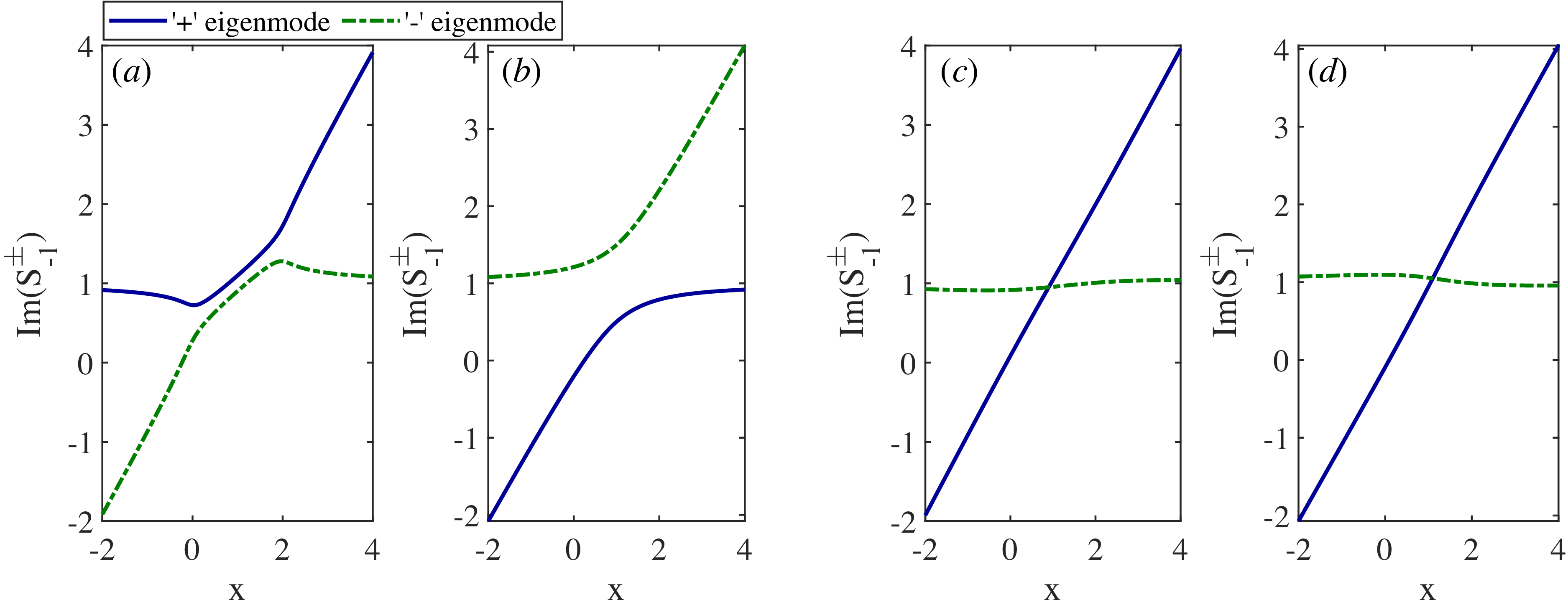
The linear wavenumber of the daughter wave ‘1’ varies linearly as
 $K_1=\epsilon x$
, whereas that of the daughter wave ‘u’ remains constant
 $K_u-K_0$
. As shown in figure 2(a,b), mode exchange occurs: for instance, in figure 2(a), the ‘+’ eigenmode behaves as the ‘u’ wave in the limit
 $x\to -\infty$
, while it evolves into the ‘1’ wave as
 $x\to +\infty$
. This exchange indicates the presence of strong Stokes jumps in the resonant PI regime. By contrast, figure 2(c,d) shows no mode exchange, suggesting that the associated Stokes jumps are weak for non-resonant regimes.
Eigenmode wavenumbers along the wave trajectory for PI regimes: (a) resonant forward scattering; (b) resonant backward scattering; (c) non-resonant forward scattering; (d) non-resonant backward scattering. These figures allow identification of which eigenmode corresponds to each daughter wave as
 $x\to \pm \infty$
.

Eigenmode evolution of resonant forward scattering in figure 3(a) differs from resonant backward scattering in figure 3(b). In the coupling region defined by the interval between the jump positions noted by red dashed lines, the eigenmodes in the resonant forward scattering regime vary quickly. In contrast, those in the resonant backward scattering merely change. For the non-resonant regimes in figures 3(c,d), the wave ‘1’ slowly varies, while the quasi-mode ‘u’ linearly damps.

Now, we discuss the four different PI regimes one by one.
4.1. Resonant forward scattering
In the resonant forward scattering regime, both daughter waves ‘1’ and ‘u’ are resonant and propagate from
 $-\infty$
to
 $+\infty$
. As shown in figure 2(a), wave ‘1’ corresponds to eigenmode ‘–’ at
 $x\to -\infty$
and ‘+’ at ‘
 $x\to +\infty$
’, while wave ‘u’ behaves inversely. Assuming the coefficients
 $c_a^\pm$
before coupling are known, the coefficients
 $c_b^\mp$
after coupling can be determined by the connection formula.
According to the Stokes diagram in figure 1(a), the wave encounters two Stokes lines and the connection formula is
 \begin{align} \left (\begin{array}{c} c_{b}^{+}\\[3pt] c_{b}^{-} \end{array}\right )=\left (\begin{array}{c@{\quad}c} 1 & 0\\[3pt] ie^{2V/\epsilon } & 1 \end{array}\right )\left (\begin{array}{c@{\quad}c} 1 & -i\\[3pt] 0 & 1 \end{array}\right )\left (\begin{array}{c} c_{a}^{+}\\[3pt] c_{a}^{-} \end{array}\right ). \end{align}
Consequently, for wave ‘1’, the Stokes jump yields
 \begin{align} c_{a}^{-}\to c_{b}^{+}=c_{a}^{+}-ic_{a}^{-}. \end{align}
However, for wave ‘u’, the jump result yields
 \begin{align} c_{a}^{+}\to c_{b}^{-}=ic_{a}^{+}e^{2V/\epsilon }+c_{a}^{-}\left (1+e^{2V/\epsilon }\right ). \end{align}
The final amplitude of one daughter wave depends not only on its incident amplitude, but also on that of the other daughter wave. Since daughter waves are typically seeded by background noise, arbitrary initial conditions
 $c_a^\pm$
may in principle be realised. Special cases, such as
 $c_a^+=ic_a^-$
, which lead to the vanishing of wave ‘1’ after coupling, are also possible. However, our physical interest usually lies in the strongly amplified daughter waves that grow from the noise floor to amplitudes large enough to affect the system dynamics. Since this requires amplification over many orders of magnitude, the relevant regime is typically of large amplification (
 $A\gg 1$
). In this limit, even a modest difference in amplification factor is exponentially magnified, such that the seed corresponding to the maximum amplification overwhelmingly dominates the final wave amplitude. Therefore, for most practical purposes, such as evaluating the PI-induced lower hybrid sidebands in tokamaks (Cesario et al. Reference Cesario, Cardinali, Castaldo, Paoletti and Mazon2004) or estimating the worst gain induced by stimulated Raman scattering in inertial confinement fusion (Rosenberg et al. Reference Rosenberg2018), it is sufficient to consider only the boundary condition that yields the maximum amplification.
In figure 4, the actual wave amplitude evolution is traced by combining the eigenmode evolution with the Stokes jumps. When focusing on the evolution of a single wave, the incident coefficient of the other daughter wave is set to zero. It can be observed that, although the final amplification predicted by the exact WKB and the conventional WKB approaches is identical, the local wave behaviours exhibit clear differences near the boundaries of the coupling region, i.e. in the vicinity of the turning points. In this region, higher-order WKB corrections become significant and the conventional WKB validity condition breaks down. Remarkably, the higher-order contributions from the two turning points cancel each other, which ultimately leads to the same prediction for the final amplification factor.
Amplitude evolution of (a) daughter wave ‘u’ and (b) daughter wave ‘1’ for resonant forward scattering PI. From the exact WKB perspective, the green solid lines represent waves with well-defined wavenumbers, while purple-shaded regions indicate intervals where the daughter waves are strongly coupled and cannot be clearly distinguished. The blue dashed lines show the amplitude evolution predicted by the conventional WKB method. The incident coefficients are
 $c_a^+=1, c_a^-=0$
for panel (a) and
 $c_a^+=0, c_a^-=1$
for panel (b).

Consistency checks of the exact WKB solutions of the original ODE (2.3) are presented in figure 5, where they are found to be in indistinguishable agreement with numerical solutions and the parabolic cylinder representation.
The
 $\phi _1$
solution of (2.3) obtained via exact WKB (solid line), a numerical ODE solver (crosses) and the parabolic cylinder function representation in (4.2) (circles) for the resonant forward scattering regime. Black curves/markers denote the amplitude of
 $\phi _1$
, while red curves/markers denote the unwrapped phase. Parameters of panels (a) and (b) are the same as those used in figures 4(a) and 4(b), respectively.

4.2. Resonant backward scattering
In the resonant backward scattering regime, wave ‘u’ propagates in the opposite direction. From the wave-vector evolution shown in figure 2(b), we identify that the ‘+’ eigenmode at
 $x\to -\infty$
and the ‘–’ eigenmode
 $x\to +\infty$
correspond to wave ‘1’, whereas the ‘–’ eigenmode at
 $x\to -\infty$
and ‘+’ eigenmode at
 $x\to +\infty$
correspond to wave ‘u’. Therefore, the two coefficients representing the incident waves are
 $c_a^+$
and
 $c_b^+$
. Indicated by the Stokes diagram in figure 1(b), the connection formula is
 \begin{align} \left (\begin{array}{c} c_{b}^{+}\\[3pt] c_{b}^{-} \end{array}\right )=\left (\begin{array}{c@{\quad}c} 1 & ie^{2V/\epsilon }\\[3pt] 0 & 1 \end{array}\right )\left (\begin{array}{c@{\quad}c} 1 & 0\\[3pt] -i & 1 \end{array}\right )\left (\begin{array}{c} c_{a}^{+}\\[3pt] c_{a}^{-} \end{array}\right )\!. \end{align}
For wave ‘1’, the Stokes jump is
 \begin{align} c_{a}^{+}\to c_{b}^{-}=ie^{-2V/\epsilon }(c_{a}^{+}-c_{b}^{+}), \end{align}
while for wave ‘u’, which propagates in the opposite direction to wave ‘1’, the Stokes jump reads
 \begin{align} c_{b}^{+}\to c_{a}^{-}=ie^{-2V/\epsilon }(c_{a}^{+}-c_{b}^{+})+ic_{a}^{+}. \end{align}
Note that in backward-scattering regimes,
 $V_r\lt 0$
because
 $v_{gu}v_{g1}\lt 0$
. Since we are only interested in the maximally amplified PI response, we focus on cases in which the large factor
 $\exp (2|V_r|/\epsilon )$
appears in the post-coupling coefficients
 $c_a^-$
and
 $c_b^-$
. Combinations such as
 $c_a^+=c_b^+$
are therefore disregarded.
The amplitudes of the
 $\pm$
eigenmodes shown in figure 3(b) vary little across space, yet the amplitude difference between the ‘+’ and ‘–’ eigenmodes becomes pronounced. This disparity arises from the
 $\mathcal{L}^{-\text{1}}\mathcal{B}[S^+]$
integral evaluated from the upper turning point in figure 1(b) to 0, together with the
 $\mathcal{S}[R^-]$
integral from the lower turning point to 0. These two contribute to an amplitude disparity approximately
 $|\phi _-/\phi _+|\simeq \exp (-|V_r|/\epsilon )$
.
Taking into account that the Stokes jump already provides an amplification of
 $\exp (-2V_r/\epsilon )$
, the final amplification factors of both daughter waves are estimated as
 $\exp (-V_r/\epsilon )$
. To confirm this precisely, figure 6 shows the amplitude evolution from the perspective of exact WKB. Again, when examining the growth of a particular daughter wave, the incident coefficient of the other wave is set to 0. The logarithmic amplitude difference between ends of the interval results in
 $7.854$
for both daughter waves, consistent with the estimated amplification factor
 $A_{\text{inhom}}=|V_r|/\epsilon$
, identical to the resonant forward scattering case. Verification of the exact WKB solution for this regime is shown in figure 7, demonstrating full consistency among all methods.
Amplitude evolution of (a) wave ‘1’ and (b) wave ‘u’ in resonant backward scattering PI. The purple shaded regions represent coupling intervals where the two daughter waves cannot be distinguished from each other. The incident coefficients are chosen as
 $c_a^+=1, c_b^+=0$
in panel (a) and
 $c_a^+=0, c_b^+=1$
in panel (b).

Comparison of the solution
 $\phi _1$
of (2.3) obtained from the exact-WKB method (solid lines), a numerical ODE solver (crosses) and the parabolic-cylinder-function representation (4.2) (circles) for the resonant backward scattering regime. Black curves/markers denote the amplitude of
 $\phi _1$
, and red curves/markers denote the unwrapped phase. Panels (a) and (b) use the same parameters as figures 6(a) and 6(b), respectively.

The
 $\exp (|V_r|/\epsilon )$
amplification appears to contradict the zero amplification predicted by (2.5). From the conventional WKB perspective, the zero amplification results from the fact that none of the phase integrands
 $\pm \sqrt {Q(x)}$
on the entire real axis possesses a real part, except for small corrections of order
 $O(\epsilon )$
.
The discrepancy originates from an intrinsic limitation of the conventional WKB method, which ignores Stokes jumps. This ignorance of Stokes jumps is equivalent to an implicit boundary condition that the amplitude of the unconcerned wave vanishes at the incident side of the concerned wave; only then can the eigenmode corresponding to the incident concerned wave evolve without a coefficient jump. In the resonant forward scattering regime, where both daughter waves propagate in the same direction, this assumption causes no issue. However, in the resonant backward scattering regime, it effectively sets the outgoing amplitude of the counter-propagating wave ‘u’ to zero. Since parametric amplification relies on a positive-feedback loop between both waves, suppressing one prevents the growth of the other, leading to the zero amplification predicted by conventional WKB. This can be verified by substituting
 $c_a^-=0$
into (4.9) and (4.10), which yields
 $c_b^-=-ic_a^+$
and a final attenuation of wave ‘1’ about
 $\exp (-|V_r|/\epsilon )$
.
As shown within the exact WKB framework, the zero amplification predicted by the conventional WKB treatment for resonant backward scattering PIs (
 $({\varGamma \varGamma ^*}/{v_{gu}v_{g1})}\lt 0$
) is invalid, due to the omission of boundary-condition data, in particular, Stokes jumps. In our previous work (Zhou et al. Reference Zhou, Xiang, Gan and Xia2025), the condition
 $\alpha \alpha ^*\lt 0$
was expressed in terms of
 $\alpha =\varGamma /v_{gu}$
and
 $\alpha ^*=\varGamma ^*/v_{g1}$
without distinguishing whether it arises from
 $\varGamma \varGamma ^*\gt 0$
,
 $v_{gu}v_{g1}\lt 0$
or
 $\varGamma \varGamma ^*\lt 0$
,
 $v_{gu}v_{g1}\gt 0$
(in the latter case,
 $\varGamma ^*$
is no longer the complex conjugate of
 $\varGamma$
). The present analysis shows that these cases lead to fundamentally different behaviours. The former, i.e. the resonant backward scattering considered here, yields finite amplification, whereas the latter corresponds to the resonant forward scattering with zero amplification. Nevertheless, the previously reported mechanism, whereby increasing the linear growth rate of the daughter wave ‘u’ in the latter regime breaks the negative feedback loop and restores PI amplification, remains applicable.
4.3. Non-resonant forward scattering
Compared with the resonant type, where the incident amplitudes of both daughter waves must be prescribed, the non-resonant regime allows a much simpler boundary condition, as the heavily damping quasi-mode cannot exist as an incident wave and is instead generated exclusively through nonlinear coupling.
Figure 2(c) shows that the ‘+’ eigenmode corresponds to daughter wave ‘1’ and the ‘–’ eigenmode corresponds to the quasi-mode ‘u’ throughout the domain, without any mode exchange as in the resonant regimes.
Given that the quasi-mode’s incident coefficient
 $c_a^-$
is zero and Stokes diagram in figure 1(c), we have the connection formula:
 \begin{align} \left (\begin{array}{c} c_{b}^{+}\\[3pt] c_{b}^{-} \end{array}\right )=\left (\begin{array}{c@{\quad}c} 1 & 0\\[3pt] ie^{2V/\epsilon } & 1 \end{array}\right )\left (\begin{array}{c@{\quad}c} 1 & 0\\[3pt] i & 1 \end{array}\right )\left (\begin{array}{c@{\quad}c} 1 & i\\[3pt] 0 & 1 \end{array}\right )\left (\begin{array}{c} c_{a}^{+}\\[3pt] 0 \end{array}\right ). \end{align}
Solving the connection formula, we find that the Stokes jump for wave ‘1’ is
 \begin{align} c_{a}^{+}\to c_{b}^{+}=c_{a}^{+}, \end{align}
while the quasi-mode’s Stokes jump yields
 \begin{align} c_{a}^{-}=0\to c_{b}^{-}=ic_{a}^{+}\left (1+e^{2V/\epsilon }\right ). \end{align}
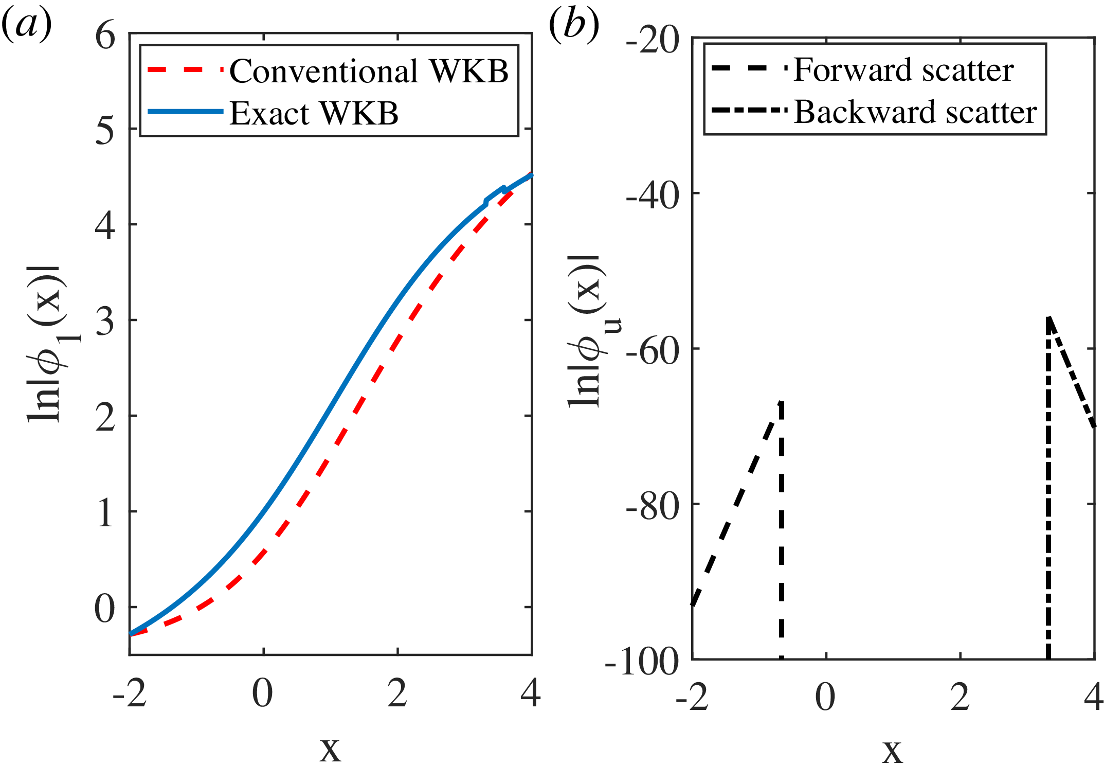
Therefore, amplification of wave ‘1’ does not depend on the Stokes jump and is entirely governed by its intrinsic spatial evolution, as illustrated in figure 8(a). Because of the absence of Stokes jump contribution and mode exchange, the conventional WKB treatment remains valid in this regime.
Amplitude evolution of (a) wave ‘1’ and (b) quasi-mode ‘u’ for non-resonant parametric instability (PI) within the exact WKB framework. The behaviour of wave ‘1’ in panel (a) is identical for forward and backward scattering; thus, only one case is shown. The conventional WKB result is included as a blue solid line for comparison. In panel (b), the quasi-mode ‘u’ exists only over part of the spatial interval, as it is generated solely through nonlinear coupling.

In the conventional WKB approach, increasing the linear spatial damping rate
 $K_{ui}$
of quasi-mode ‘u’ causes the effective growth rate to spread across the entire real axis, rather than remaining localised between the turning points. Consequently, the integral evaluated over a finite region becomes smaller than the standard value
 $V_r/\epsilon$
.
We also compare the conventional WKB prediction with the evolution obtained from the exact WKB analysis in figure 8(a). The final amplification factor of daughter wave ‘1’ between a fixed spatial interval is found to be identical in both approaches. Although the higher-order WKB terms included in the exact WKB framework modify the local amplitude, these contributions are axially symmetric about the midpoint between the two turning points, and thus their net contribution to the integral over the entire interval vanishes.
The evolution of the quasi-mode is shown in figure 8(b). It is triggered by a Stokes jump at the second crossing point, with an amplitude much smaller than wave ‘1’, and quickly decays due to strong linear damping. This may account for the difficulty in experimentally detecting the quasi-mode. Figure 9(a) compares exact WKB solutions in this regime with other methods, showing that the results of all the approaches are numerically distinguishable.
Comparison of the solution
 $\phi _1$
of (2.3) obtained from the exact-WKB method (solid lines), a numerical ODE solver (crosses) and the parabolic-cylinder-function representation in (4.2) (circles). Panel (a) is the non-resonant forward scattering PI regime, while panel (b) is the non-resonant backward scattering. Black curves/markers denote the amplitude of
 $\phi _1$
and red curves/markers denote the unwrapped phase. The linear growth trend observed in the parabolic cylinder representation and numerical solution in panel (b) indicates the onset of numerical stability.

4.4. Non-resonant backward scattering
Finally, the results in the non-resonant backward scattering case are nearly identical to those of the non-resonant forward scattering case. The key difference is that the quasi-mode ‘u’ propagates and damps in the negative
 $x$
-direction, leading to the boundary condition
 $c_b^-=0$
.
The connection formula based on Stokes diagram in figure 1(d) is
 \begin{align} \left (\begin{array}{c} c_{b}^{+}\\[3pt] 0 \end{array}\right )=\left (\begin{array}{c@{\quad}c} 1 & -ie^{2V/\epsilon }\\[3pt] 0 & 1 \end{array}\right )\left (\begin{array}{c@{\quad}c} 1 & 0\\[3pt] -ie^{-2V/\epsilon } & 1 \end{array}\right )\left (\begin{array}{c@{\quad}c} 1 & 0\\[3pt] -i & 1 \end{array}\right )\left (\begin{array}{c} c_{a}^{+}\\[3pt] c_{a}^{-} \end{array}\right ). \end{align}
The Stokes jump of wave ‘1’ is the same as (4.12), indicating no contribution to PI amplification. The Stokes jump of quasi-mode ‘u’ is given by
 \begin{align} c_b^-=0\to c_a^-=ic_a^+(1+e^{-2V/\epsilon }). \end{align}
The intrinsic amplitude evolution of wave ‘1’ is the same as in the non-resonant forward regime shown in figure 8(a). As shown in figure 8(b), the quasi-mode ‘u’ is generated at the crossing point
 $P_2$
in figure 1(d), with again an amplitude that remains negligibly small and rapidly decays due to linear damping.
Cross-validation for this regime is presented in figure 9(b). The numerical solution becomes unstable beyond
 $\text{Re}(x)=-0.74$
, as the quasi-mode exponentially amplifies the small numerical errors during propagation toward increasing x. The analytical solution based on parabolic cylinder functions also breaks down beyond
 $\text{Re}(x)=1.08$
, where severe cancellation occurs between the two large contributions satisfying
 $c^{[1]}\phi _1^{[1]}\simeq -c^{[2]}\phi ^{[2]}_1$
. In contrast, the exact WKB solution remains stable throughout the entire domain, maintaining a well-behaved amplitude and phase without any sign of breakdown. This demonstrates the superior robustness of the exact WKB approach compared with both direct numerical integration and analytical representations via special functions.
5. Conclusions and discussions
In this work, the exact WKB method is employed to examine the coupled daughter-wave equations governing various types of convective parametric instability (PI) in inhomogeneous plasmas, including both resonant and non-resonant regimes as well as forward scattering and backward scattering regimes. While this problem has been previously studied by Zhou et al. (Reference Zhou, Xiang, Gan and Xia2025) within the conventional WKB framework, we revisit it here using the exact WKB approach to overcome several limitations inherent in the conventional WKB treatment.
Compared with the conventional WKB approach, the exact WKB method offers two key advantages. First, it is not restricted by the WKB validity conditions and can be systematically applied to ODEs with spatially varying coefficients at arbitrary order. Second, it naturally incorporates the boundary conditions, whereas conventional WKB typically tracks only the integral of a single eigenvalue, thus failing to capture the effects of Stokes jumps.
From the exact WKB perspective, the amplification of the daughter waves arises from two mechanisms: the Stokes jumps and the intrinsic spatial evolution of the eigenmodes. As a result, the amplification factor of all four types of PI is found to be
 \begin{align} A_{\text{inhom}}=|V_r|/\epsilon =\dfrac {\pi |\varGamma |^2}{\epsilon |v_{gu}v_{g1}|}, \end{align}
where it depends on the coupling coefficient
 $\varGamma$
, the group velocities
 $v_g$
of the daughter waves and the strength of inhomogeneity
 $\epsilon$
. The term
 $V_r$
originates from the real part of the Voros multiplier, namely the contour integral around the turning points. Variations in the PI regime merely induce global translations or rotations of the Stokes diagram and therefore do not affect the value of
 $V_r$
.
As a complementary remark, we briefly comment on certain resonant PI regimes that lie outside the noise-seeded large-amplification regime primarily considered in this work. In these cases, the amplification remains small, and both daughter-wave incident amplitudes are explicitly specified. The amplification factor then becomes additionally dependent on the initial amplitude ratio. Using the Stokes jump relations in (4.6) and (4.9), as well as their eigenfunction evolution shown in figure 3(a,b), the amplification factor is corrected as
 $|V_r|/\epsilon +\ln |c_1-ic_u|-\ln |c_1 |$
, where
 $c_1$
and
 $c_u$
are initial coefficients of wave ‘1’ and ‘u’, respectively.
Results previously obtained using the conventional WKB approach are also corrected by the exact WKB method. Owing to its inability to account for Stokes jumps, the conventional WKB treatment predicts zero amplification for resonant backward scattering PI, as indicated by (2.5). In contrast, the exact WKB analysis shows that Stokes jumps dominate the amplification in this regime, yielding an amplification factor
 $|V_r|/\epsilon$
.
It is noteworthy that the present study primarily serves as an initial demonstration of the applicability of the exact WKB method to the analysis of PIs. More complex scenarios, such as the influence of daughter-wave reflection or mode conversion on the PI process governed by a third-order ODE or higher, can in principle be treated within the exact WKB framework, but are not considered in the present revisit and will be addressed in future work.
While such more complex scenarios are not included in the present analysis, the effect of strong plasma inhomogeneity for PIs described by (2.1) and (2.2) can already be examined within the current framework. As long as the governing ODE can be reduced to a Weber equation like (4.1), its amplification factor is universally inversely proportional to the parameter gradient
 $\epsilon$
, regardless of the value of
 $\epsilon$
. The Voros multiplier
 $V$
is independent of
 $\epsilon$
because the net contribution of the higher-order WKB terms vanishes, yielding
 \begin{align} V=\dfrac {\epsilon }{2}\oint _I \mathcal{L}^{-\text{1}}\mathcal{B}[S^+-S^-]{\rm d}x=\dfrac {1}{2}\oint _I (S^+_{-1}-S_{-1}^-) {\rm d}x. \end{align}
For more complex systems, such as higher-order ODEs or Schrödinger-type equations with polynomial potentials
 $Q(x)$
containing quartic terms, the associated Picard–Fuchs equation for
 $V$
generally has differential order higher than one. In such cases, the Voros multiplier exhibits a non-trivial dependence on the inhomogeneity parameter
 $\epsilon$
. These more intricate scenarios will be systematically investigated within the exact WKB framework in future work.
Acknowledgements
Editor Louise Willingale thanks the referees for their advice in evaluating this article.
Funding
This work was supported by the Hundred Talents Program of the Chinese Academy of Science, the Strategic Priority Research Program of Chinese Academy of Sciences (Grant Nos. XDB0790000 and XDB0500302) and the National Natural Science Foundation of China (Grant Nos. 12375231 and 12575245).
Declaration of interests
The authors report no conflict of interest.


 Pj
 x→±∞


 ca+=1,ca−=0
 ca+=0,ca−=1

 ϕ1
 ϕ1

 ca+=1,cb+=0
 ca+=0,cb+=1

 ϕ1
 ϕ1

 ϕ1
 ϕ1

 Open access

