


Politics is replete with principal-agent relationships. Research often conceptualizes politicians, bureaucrats, and courts as agents of their own principals and models the principal as the rule-making body and the agent as the implementing body. Electorates elect politicians based on a policy mandate that they are expected to implement once in office; executives appoint bureaucrats to implement the laws of the land; lower courts implement the rules dictated by upper courts. Yet, principals often delegate to their agents the authority to make the rules themselves. For example, in the United States, bureaucracies such as the Food and Drug Administration and the Environmental Protection Agency (EPA) are often charged with rule-making responsibilities, but are subject to oversight by Congress and the courts.
The judicial hierarchy is a particularly important example of this phenomenon. Judge-made law constitutes a large portion of the rules that affect the daily lives of most people in the United States. Courts make law on such important constitutional matters as whether public education may be segregated along racial lines and on more routine matters such as the conditions that constitute wrongful termination. Because of its position at the apex of the judicial hierarchy, the Supreme Court is usually the focus of the study of judge-made law. That focus, however, misses how a substantial amount of judge-made law is created in the United States. The Supreme Court hears only a very small fraction of the cases filed in federal courts (about 0.02%); most law is both made and applied in the lower courts, especially the federal courts of appeals. Indeed, the Supreme Court is often guided by law that has previously been created by lower courts.Footnote 1
To the degree that lower courts appear in theories of judicial lawmaking, they are usually treated as subordinate institutions responsible only for implementing rules generated by the Supreme Court. Scholars examine issues such as whether and to what degree lower courts deviate from applying the rules generated by the Supreme Court and under what conditions the Supreme Court reviews and reverses lower court decisions (e.g., Cameron, Segal and Songer Reference Cameron, Segal and Songer2000).
In this article we develop and test a theory of rulecreation and application in which the lower court is explicitly allowed to formulate its own rules, subject to possible review by an upper court. Introducing the ability of lower courts to choose rules as well as to decide cases allows us to answer three unexplored questions about law creation in a judicial hierarchy. First, how do characteristics of a case (i.e., the facts of the case, its importance, and the degree to which the lower and upper court have differing preferences over what rules should govern the relevant body of law) affect the rules the lower court will choose? Second, under what conditions is the upper court more likely to review the lower court's decision in light of the rule the lower court declares? And third, how is the upper court likely to treat the lower court's decision—the way a lower court decides a case and the rule used to justify that decision?
Several our theoretical findings represent surprising and normatively important relationships in answer to these questions. For example, the facts of a case can significantly influence the rule the lower court declares, and therefore the merits of the case can potentially substantially influence the future direction and content of judge-made law. Further, surprisingly, at times the upper court intentionally allows the lower court to establish rules that are relatively distant from the upper court's preferred rule and (seemingly ironically) potentially reviews and reverses decisions that appear, on the surface, far more consonant with the upper court's preferences. This theoretical finding has important implications for the extent to which Supreme Court preferences over law determine how U.S. law is actually made and applied. Finally, we find non-monotonic relationships between the ideological divergence of the lower court from the upper court and the likelihood of both review and reversal by the upper court. This finding is novel and has substantial implications for the Supreme Court's influence on the application of law. We find empirical support for this last pair of theoretical predictions.
PREVIOUS APPROACHES
Past research in this area has focused most directly on how or to what extent judges higher in the hierarchy—e.g., the Supreme Court—can control or influence the decisions made by judges lower in the hierarchy. Rather than examining the rule-making function, it has focused on error correction (for a discussion, see Friedman Reference Friedman2006). Research has demonstrated that, when lower courts disregard their superiors’ preferences, they are more likely to be reviewed (e.g., Cameron, Segal, and Songer Reference Cameron, Segal and Songer2000; Clark Reference Clark2009). The operative assumption is that higher courts seek strategically to audit lower courts in an effort to “catch” those cases that it finds most displeasing. Recent studies of the rule-creation function of superior courts have examined the review strategies that they use to exercise control over the large bureaucracy of lower courts that interprets and applies those rules (e.g., Jacobi and Tiller Reference Jacobi and Tiller2007; Lax Reference Lax2009; Staton and Vanberg Reference Staton and Vanberg2008). This research characterizes rule making in a political hierarchy as a classical moral hazard problem (see also McNollgast 1995).
We approach the principal-agent problem from the bottom up, focusing on the role lower courts play in rule making. Although much of the research on lower courts has centered on the votes that lower court judges cast (e.g., Hettinger, Lindquist, and Martinek Reference Hettinger, Lindquist and Martinek2006), scholars lately have been paying greater attention to the role judges play in the construction of law.Footnote 2 In the most detailed study, Klein (Reference Klein2002) examines the creation of legal rules by circuit courts in the absence of guidance from the Supreme Court. Klein considers cases where the Supreme Court has not offered an authoritative legal rule to govern a situation (cases of first impression). Although he does not develop an explicit theory of intercourt interactions, Klein argues that the extent to which a judge adopts an existing rule depends critically on whether the judge is in sympathy with that rule. Importantly, however, Klein argues that judges on the court of appeals are not influenced by the anticipated preferences of the Supreme Court when deciding a case of first impression. From a different, purely theoretical perspective, Hammond, Bonneau, and Sheehan (Reference Hammond, Bonneau and Sheehan2006) develop a trio of formal models they use to investigate how the Supreme Court's internal bargaining process influences the policies that the lower courts will adopt, as well as the conditions under which the lower courts can exercise greater or lesser influence over the law. Their analysis centers on the policy choices that lower courts will make under the shadow of oversight by the Supreme Court.
Because (a) most law is created in the courts of appeals and (b) cases enter the system in the lower courts, which have the first opportunity to resolve them, we approach the problem of rule creation in a hierarchy from the perspective of the lower courts. In the next section, we advance a series of formal models of law creation in a judicial hierarchy characterized by an informational asymmetry (i.e., lower courts are better informed about cases than are higher courts, which have not reviewed them). We then discuss the implications of our model and present empirical support for two of the predictions.
THE MODELS
Our models build from canonical principal-agent models. In particular, consistent with Cameron, Segal, and Songer (Reference Cameron, Segal and Songer2000), we assume that a lower court hears a case with specific case facts and must determine the case's outcome. The upper court observes the lower court's decision, but does not observe the case facts unless it chooses to review the lower court's decision. Reviewing the lower court's decision requires paying some cost in time and resources but, in exchange, allows the upper court to learn the case facts and dictate its preferred outcome. Unlike Cameron, Segal, and Songer, we allow the lower court both to declare a rule and dispose of the case.Footnote 3 The rule is observable to the upper court before it decides to grant or deny certiorari, and therefore it potentially provides information that the upper court can use when deciding whether to hear a case. On reviewing the lower court's decision, the upper court can change the rule used in the case, thereby potentially changing the case's disposition (i.e., reversing the lower court). A final key feature of our model is that, whereas most models of judicial hierarchy assume that there is some exogenous cost associated with the displeasure of being reversed (beyond the policy implications; e.g., Kastellec Reference Kastellec2007), we do not assume such a cost. Rather, any reduction in the lower court's utility from review arises as a function of the degree of ideological divergence between the upper and lower courts and the actions that the two courts take.
The primary source of incomplete information between the courts in our model is the contextual nuances of an individual case (the case facts), rather than the courts’ preferences or the actions they have taken (rules and dispositions). We focus on uncertainty about case facts for three reasons. First, judges have a close, long-lived working relationship, both within and across levels of the hierarchy (e.g., Hammond, Bonneau, and Sheehan Reference Hammond, Bonneau and Sheehan2006, 137). Thus, they are likely to have an appreciation of each others’ preferences. Second, their actions are public and the subject of written documentation. Before deciding whether to review a case, the upper court justices are likely to have a fairly clear idea of how a case was decided and why. Third, by contrast, many cases come to the courts that present similar issues and problems, even though the specifics of the cases are always unique. Thus, the nuances of a given case are going to be comparatively hard to assess until it is actually heard. Our assumption of uncertainty about case facts does not, however, imply that the upper court is completely unaware of the case's context or issues. Rather, it implies that, until the upper court agrees to review a case, the lower court has an informational advantage on the particulars of the case and which disposition a given rule might induce.
Our baseline model is of a nonstrategic lower court, one that does not care about subsequent moves made by the Supreme Court and therefore is not influenced by the institutional structure of the hierarchy; this model serves as a benchmark against which we can compare behavior in subsequent extensions. We then introduce a strategic element—we allow the lower court to have preferences over the decisions made by its superior court. This court is similar to those in most models of judicial auditing (e.g., Cameron, Segal, and Songer Reference Cameron, Segal and Songer2000; Clark Reference Clark2009).Footnote 4 Finally, we extend our model by introducing an additional informational asymmetry, assuming that the lower court is uncertain about the cost to the higher court of reviewing its decision. One can interpret this uncertainty as the cost of reviewing a case in terms of resources or interest in the issue (e.g., Clark and Strauss Reference Clark and Strauss2010). Proofs and supplemental results are presented in the Appendix.
Model 1: A Nonstrategic Lower Court
Players and Sequence of Play
We model law creation in the judicial hierarchy as a game between two players, the Upper Court (UC) and the Lower Court (LC), with commonly known “ideal rules” on the real number line, U and L, respectively. We assume, without loss of generality, that U = 0 and L > 0. First, Nature draws the case facts from a unidimensional fact-space. Formally, the case facts are represented by a point on the real number line,  . LC observes f, but UC does not. Second, LC chooses a rule, r, which maps the fact-space into a dichotomous disposition-space.Footnote 5 Third, UC observes r and the resulting disposition and must decide whether or not to audit LC's decision. If UC audits the decision, it observes f (resolving the information asymmetry) and is free to select a new rule it chooses.
Strategies
A strategy for the Lower Court is a rule,  ; a strategy for the Upper Court is a pairing of an audit probability and a rule to select on auditing, 〈a(r), rUC〉. Because the Upper Court always has a dominant strategy to select its ideal rule (rUC = U = 0) on review, we collapse the Upper Court's strategy into a single choice: the probability of auditing the Lower Court, a(r). Throughout this article, we use search-and-seizure cases as a stylized example. The fact-space represents the “intrusiveness” of a search; the disposition-space is the decision either to admit or exclude the evidence from the search. Specifically, a rule divides the fact-space into dispositions so that all cases with f ≥ r are placed into the “exclude” disposition, and all cases with f < r are placed into the “admit” disposition.Footnote 6 One can think of the intrusiveness of the search as the extent to which the police invade one's privacy. A very intrusive search is one in which the police knock down the door to one's home and turn the house upside down looking for something without a warrant or probable cause. A less intrusive search might be one in which a police officer approaches a car that has been stopped for a traffic violation and asks the driver if he may inspect the trunk of the car and the driver consents. A rule is a point along the continuum from least intrusive to most intrusive searches at which the court decides that evidence obtained from searches that are less intrusive than that point is admissible and evidence from more intrusive searches is not admissible. The fact- and disposition-spaces are shown visually in Figure 1. Many rules may lead to the same disposition of any given case. For example, in a intrusive search (one with f very far to the right along
 ), there are many rules to the left of f, which would all yield the “exclude” disposition.
Visual Representation of the Case-space Model
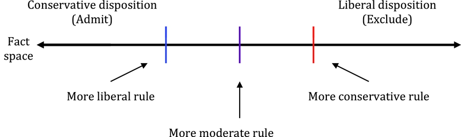
To understand the relationships among rules, facts, and dispositions, consider the following example. In U.S. v. Katz (1967), the Supreme Court was asked to consider whether warrantless wiretapping constitutes an unconstitutional search. The Court had previously chosen a rule in Olmstead v. U.S. (1928), which held that electronic eavesdropping without a warrant did not constitute an impermissible search. In Katz, however, the Court decided that warrantless wiretapping does constitute an unconstitutional search. Thus, the Court in Katz chose a rule that was further to the left than the rule in Olmstead—the Katz rule implied that a greater range of searches were too invasive to have their evidence placed into the “admit” category. In other words, the Katz rule is one to the left of the Olmstead rule, taking cases that would have been mapped into the “admit” disposition and now mapping them into the “exclude” disposition. In this example, the warrantless wiretap constitutes the facts of the case (i.e., the level of intrusiveness), though the two cases do differ in the precise location of the case facts (the exact nature of the search). The Olmstead and Katz rules constitute the rules that decide which disposition should be given to that set of facts.
Beliefs
The source of uncertainty is the facts of the case, f. Formally, UC's uncertainty about f is characterized by a belief that f is distributed across the fact-space according to an unbounded distribution g(·). For any rule selected by the Lower Court, this uncertainty induces a potential uncertainty about whether the disposition produced by the Lower Court's rule corresponds to the disposition that would be produced by the Upper Court's ideal rule. Let b(r) represent UC's belief that the disposition announced by LC and, induced by rule r, corresponds to UC's preferred disposition.
Utilities
The two players receive utility from the rules they select and whether the resulting disposition results in his or her preferred disposition. A player's ideal rule defines her preferred disposition. Specifically, a player with ideal rule i receives −(i − r)2 from selecting rule r; each player also receives positive utility, φ>0, if the disposition induced by her selected rule accords with her preferred outcome. In other words, we assume each player receives additive utility from the two components of a decision—the rule and the case disposition. We have assumed a nonstrategic lower court: LC's utility is not affected by any change either to the rule or disposition by UC or any other consequence of being reversed, such as the professional cost of being rebuked by the Supreme Court. Finally, we also assume that UC must pay a cost, k, to audit LC's decision.Footnote 7 This cost represents an opportunity or effort associated with auditing the Lower Court; it can also capture other nonspatial features of a case, such as its political or legal salience. The more important (salient legally or politically) the case, the smaller k. We are implicitly assigning a weight of 1 to the rule. The values of φ, k, and the ratio of those two parameters therefore tell us the relative weights of the rule, disposition, and the costs of review for the courts. The smaller φ and/or k, the greater relative importance of the legal rule to the courts.Footnote 8 Each court's utility is an additive combination of the two (Lower Court) or three (Upper Court) relevant components.
Equilibrium
The solution is a unique perfect Bayesian equilibrium in which the Lower Court always chooses its ideal rule and the Upper Court reviews the decision if it finds the rule sufficiently unattractive (i.e., far away from its own ideal rule). What constitutes a sufficiently far away rule is a function of (a) the cost of reviewing the Lower Court, k, and (b) the Upper Court's belief that it dislikes the disposition (it may still be uncertain whether it agrees with the disposition; i.e., whether f falls between LC's rule and UC's ideal rule). The two courts’ optimal behavior is driven entirely by our assumption that the Lower Court is nonstrategic and therefore does not care about any move the Upper Court might make.
Proposition 1(Nonstrategic Lower Court Equilibrium).The Lower Court's strictly dominant strategy is always to set the rule at its ideal point. The Upper Court reviews the case if the rule is sufficiently far away from the Upper Court's ideal rule to justify the cost of review.
Comparative Statics
The nonstrategic model yields a series of comparative statics. First, the Upper Court is (weakly) more likely to review a decision when the costs of review (k) are smaller,Footnote 9 the Upper Court values the disposition (φ) more, or the preference divergence between the Upper and Lower Court is larger (as L increases). Second, the Upper Court is also more likely to reverse a decision when the preference divergence between the courts is larger. As L increases, the range of cases for which the courts disagree about the disposition increases, and therefore a review is more likely to yield a reversal.
Although these predictions are highly intuitive and, in some cases, essentially guaranteed by the strong assumptions we have made about the lower court's preferences, they serve two important functions. First, they establish a benchmark against which we can compare the predictions of our subsequent models. Second, as will become apparent later, they reveal that some of the most common empirical tests in the literature may not be discriminating among competing theories of judicial hierarchy.
Model 2: A Strategic Lower Court
We now consider the possibility of a strategic Lower Court. The only distinction between the strategic lower court model (SLCM) and the nonstrategic lower court model (NSLCM) is that we now assume that the Lower Court cares about the final disposition and legal rule ultimately applied in its case. That is, the Lower Court's utility is now determined by both its decision and its interaction with the Upper Court.
Players, Sequence of Play, and Beliefs
The players, sequence of play, and information environment are identical to the baseline model.
Utilities
UC's sources of utility and its utility function are identical to the baseline model. LC's utility, however, now depends on UC's moves. Rather than deriving utility from the rule it selects, LC receives utility from the rule and disposition standing at the end of the game. That is, LC receives −(L − x)2, where x is either the rule selected by LC, if UC does not audit the decision, or the rule selected by UC if UC audits the decision. LC receives φ if and only if the disposition at the end of the game corresponds to LC's preferred disposition. All components of the utility functions are additive.
Equilibrium
To solve the model, we identify the set of isomorphic pure-strategy perfect Bayesian equilibria—there is a set of equilibria in which the Upper Court and Lower Court strategies are essentially identical functions of the case facts, but the precise rule selected depends on the precise facts of the case.Footnote 10 The set of equilibria is summarized next and illustrated in the left-hand panel of Figure 2. In Figure 2a and the statement of Proposition 2, we restrict attention to the case where  , because this condition gives rise to the fullest range of possible equilibrium behavior. In the Appendix, we derive the full equilibrium and behavior without restriction on L. All equilibrium behavior discussed later holds independent of the relative location of L, and where relevant, we discuss the implications of
 .
Equilibrium Rules in Models 2 (Strategic Lower Court Model) and 3 (Stochastic Cost of Review Model) as a Function of Case Facts

Depending on the case facts, one of three outcomes obtains. When a search is not intrusive (i.e., case facts are far to the left in Figure 2a, f < ra) the lower court sets a rule at r* = ra. For moderately intrusive searches (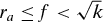 ), the Lower Court sets the rule at the case facts (r* = f), and when the search is sufficiently intrusive (
 ), the Lower Court sets the rule at
 . (As we demonstrate in the Appendix, if L < r* then the Lower Court sets the rule at L.) The disposition is a direct consequence of the rule, so the disposition is Admit if r* = ra and Exclude otherwise. The Upper Court never reviews the Lower Court. This solution characterizes a set of equilibria because ra can take on any value between r and r (we define these boundaries later). That is, the Lower Court and the Upper Court can arbitrarily coordinate on any
 .
To provide intuition for this equilibrium, we first discuss the choice of rule and then the Upper Court's decision not to review. All else equal, a Lower Court prefers a rule closer to its ideal point than further away, and it prefers a rule that yields its preferred disposition over one that does not. The further the Lower Court's ideal rule from the Upper Court's ideal rule, however, the greater the chance that the rule does not produce the Upper Court's preferred disposition (i.e., there is a larger range of case facts for which the two courts disagree about the disposition). Consequently, the Upper Court has a stronger incentive to review the case. If the Upper Court reviews the case, the Upper Court's dominant strategy is to set the rule at its ideal point, which can cost the Lower Court its preferred disposition if the case facts lie between the courts’ ideal rules. This result illustrates the following strategic tension: The Lower Court prefers to avoid review, because review always leaves the Lower Court worse off. Avoiding review requires one of two strategies. One is for the Lower Court to offer a rule that the Upper Court prefers not to review even though the Upper Court is unsure if it is getting its preferred disposition. The alternative strategy is for the Lower Court to reassure the Upper Court that it is getting its preferred disposition so that the Lower Court can pull the rule closer to its ideal point, which means selecting the best rule it can and still yield the Upper Court's preferred disposition.
Now return to Figure 2a. Lower Courts with case facts f ≤ 0 want the same disposition as the Upper Court, Admit. These Lower Courts ideally would like to take advantage of this situation by signaling that the case disposition corresponds to the Upper Court's preferences and selecting a comparatively favorable rule (from the Lower Court's perspective). An optimal rule under this strategy would be one the Upper Court would have no incentive to review. However, any Lower Court with case facts between the Upper Court's ideal point and the declared rule would want to mimic this rule if the Upper Court is not going to review it. Doing so would again produce a disposition of Admit, but this time only the Lower Court wants this disposition. As a result, the Upper Court is going to be unsure if it agrees with the disposition induced by the Lower Court's rule. Lower Courts with case facts f ≤ ra will pool on a rule in the set r to r. Specifically, let r be the rule the Upper Court does not review even if it knows it is getting the undesired disposition and r be the rule the Upper Court is indifferent over reviewing, given all Lower Courts with case facts less than r are pooling on that rule.Footnote 11 There exists an equilibrium for any ra ∈ [r, r]. In equilibrium, when the Upper Court observes that the Lower Court plays r = ra and the disposition Admit, the Upper Court has beliefs that make it weakly prefer to not review the case.
This strategy is not feasible for f > ra. If the Upper Court observes r > ra and Admit, the Upper Court would prefer to review the case. Thus, Lower Courts with case facts greater than ra make a different choice. If these courts choose the rule ra they will produce the disposition Exclude. Because the Upper Court knows that the Lower Court wants a more permissive standard (i.e., a rule that leads to more Admit dispositions), the Upper Court knows it wants Exclude whenever the Lower Court makes that determination. Thus, the Lower Court is in a position to choose a more favorable rule than ra. In fact, the Lower Court can choose any rule that produces the Exclude disposition up to one that the Upper Court would review solely to bring the rule back into line,  . (The Upper Court prefers to pay the cost of review, k, to move any rule
 to its own ideal rule, regardless of the disposition.) If the case facts are less than
 , the Lower Court sets the rule at f (any rule to the right of f would produce the Admit disposition and get reviewed). If
 , the best the Lower Court can do is to set the rule at
 ; any rule greater than
 will always be reviewed. In each case, however, if the Lower Court can select its preferred rule and reach an Exclude disposition (i.e., if L ≤ f), then the Lower Court will select its preferred rule. As the Lower Court's ideal point, L, approaches the Upper Court's ideal point, 0, the range of case facts for which the Lower Court can select its ideal point expands and overtakes the regions where the Lower Court must concede somewhat on the legal rule.
To develop a substantive intuition for how the Lower Court might choose to balance a trade-off between the rule used and the case disposition, consider the question of whether to allow a warrantless search of a mobile home. This issue arose in a series of court of appeals decisions during the 1980s. The primary issue at stake was to determine which mobile homes should be treated like homes and which should be treated like cars for the purposes of a search. In terms of our model, the question is where in the fact-space to divide cases into those in which a warrantless search is permissible (“admit” disposition) and those in which a warrantless search is impermissible (“exclude” disposition). The Sixth Circuit Court of Appeals had an opportunity to weigh in on this issue in U.S. v. Markham (1988). In that case, the Court had to decide whether to allow a warrantless search of a mobile home. The mobile home was from out of state, had license plates on it, and had no utilities connected. The court of appeals allowed the search (it chose the more conservative “admit” disposition), but in doing so it adopted a more liberal rule than was necessary to reach the conclusion. In particular, the court held that if obtaining a warrant is not an unreasonable burden, then the law enforcement officials should do so. However, in this case, the facts were sufficiently inoffensive—the mobile home was clearly more of a car than a home—that a warrant was not necessary. The rule it used to reach that disposition was a more liberal rule than it needed to be, because it stated that under different circumstances, where the mobile home was more of a home than a car, law enforcement officials should seek to obtain a search warrant if possible. The court of appeals could have opted for a more conservative rule that simply held that searches of mobile homes fall under the “automobile exception” and do not require a warrant and still reached the “admit” disposition. This is notable, because the court of appeals panel was composed of three Reagan appointees who may reasonably have believed the Supreme Court was more liberal than the panel. In fact, in its opinion, the court of appeals explicitly noted the more liberal views of the Supreme Court, citing Justice Stevens’ dissent in a previous mobile home search case. Thus, this example illustrates how the more conservative lower court adopted a relatively liberal rule while reaching a conservative disposition, thereby trading off the disposition and rule components of its decision. The Supreme Court denied a petition for certiorari in this case.
Notice that the Upper Court never reviews in equilibrium. When case facts are to the left of ra, the Lower Court pools on a rule that the Upper Court prefers not to review, even though the Upper Court is unsure whether it agrees with the disposition induced by the Lower Court's rule. When case facts are to the right, the Lower Court and Upper Court know that they agree on the disposition. The Lower Court uses this slack to declare a rule that is as close to its ideal point as possible, but that the Upper Court still prefers not to review. Thus, the threat of review shapes the rule the Lower Court will apply. Because the Lower Court can perfectly anticipate the Supreme Court's decision, it can always choose a rule that is immune from review.
Proposition 2(Strategic Lower Court Equilibrium).In any equilibrium to the SLCM, the rule selected by the Lower Court depends on the facts of the case. For case facts far enough to the left, the Lower Court pools on a rule that yields the “admit” disposition. For middle-range case facts, the Lower Court chooses a unique rule for each value of the case facts, where the rule yields the “exclude” disposition. For case facts far enough to the right, the Lower Court pools on the best rule the Upper Court will not review, which yields the “exclude” disposition. In equilibrium, the Upper Court never reviews the Lower Court decision.
Model 3: Uncertainty about Upper Court Preferences
Although no review happens in equilibrium in the SLCM, we might easily imagine that review could happen if the Lower Court were uncertain about the Upper Court's preferences. Indeed, a standard feature of principal-agent models is that increasing uncertainty about the principal's preferences increases the chance of auditing. Simply assuming that observed review is a function of such uncertainty, however, is insufficient. Specifically, we desire to know two things. First, in what ways does review vary with such uncertainty? Second, and more important for our purposes, how might such uncertainty affect the law-creation choices made by the Lower Court? To answer these questions, we allow for uncertainty about Upper Court preferences by assuming that the Upper Court's cost to review a case is unknown to the Lower Court.Footnote 12
As we demonstrate, Lower Court behavior in this model is almost identical to Lower Court behavior in the SLCM. The purchase from the stochastic cost of review model (SCRM) concerns Upper Court behavior. Whereas in the SLCM review never occurs because the Lower Court can anticipate the Upper Court's preferences perfectly and so can avoid review, the SCRM allows auditing to take place in equilibrium. As we describe later, we derive not just the possibility of review but also a variety of counterintuitive equilibrium relationships in the use of review.
Players, Sequence of Play, and Beliefs
The players and sequence of play in this model are essentially the same as in the preceding model, except that we now assume that the model begins with Nature drawing a “type” for the Upper Court. Specifically, Nature selects i ∈ {l, h}, which is private information to the Upper Court. The Upper Court's type determines the Upper Court's cost to review a Lower Court decision. Substantively, an Upper Court with low review costs can be thought of as a Court that cares a great deal about a case below or finds that reviewing a case is less taxing of its resources (not that the disposition or rule is more valuable but simply that the effort associated with reviewing the case is less).Footnote 13 The Upper Court's uncertainty about the facts of the case is characterized by the same beliefs as described earlier. The Lower Court's uncertainty about the Upper Court's type, i, is characterized by a belief  .
Utilities
The Lower Court's utility function is the same as in the SLCM. The Upper Court's utility function is the same except that the cost of reviewing a Lower Court decision is now indexed by the Upper Court's type, with kl < kh.
Equilibrium
To solve the model, we again identify the set of isomorphic pure-strategy perfect Bayesian equilibria.Footnote 14 The set of equilibria is characterized in Figure 2b.Footnote 15 As in the previous model, we again restrict attention to the case where  in the formal statement of the equilibrium and Figure 2b. We also assume a particular ordering of the various cutpoints; these restrictions are for illustrative purposes and do not affect the equilibria or their substantive interpretation.
As Figure 2b reveals, the strategies are isomorphic to the equilibrium strategy from the SLCM. The critical difference is that, if the Lower Court believes it is sufficiently likely that the Upper Court is a high-cost type (that is, p is sufficiently low), then the Lower Court will play the risk-seeking strategy that involves choosing a rule that an Upper Court with low costs would review. The intuition behind this result is straightforward: If the Lower Court believes the Upper Court is a high-cost type, then it will be willing to play a strategy that the high-cost type would find acceptable, but the low-cost type is willing to pay the cost to review.
Consider first Regions I and II in Figure 2b. In these regions, the Lower Court always pools on a rule—which rule it pools on is determined by the Lower Court's decision to pursue either the risk-seeking or risk-avoiding strategy. If it pursues the risk-seeking strategy (the dotted line), review occurs with positive probability. Sometimes the Upper Court will reverse the Lower Court (Region II), but sometimes it will affirm the Lower Court (Region I). The logic here is that the Upper Court is strategically auditing these cases—it prefers to review the case when it believes it is sufficiently likely that it has not received its preferred disposition. As in all situations of auditing under incomplete information, there will be instances in which the Upper Court reviews and learns that it would have preferred not to review (i.e., it prefers not to reverse the Lower Court). If the Upper Court had known it was receiving its preferred disposition (i.e., f<0), then it would have been willing to accept the Lower Court's rule.
In Region III, a Lower Court playing the risk-avoiding strategy will switch from the pooling strategy to the separating strategy, giving the Upper Court its preferred disposition while choosing the best rule it can (from its own perspective) to reach that disposition. Meanwhile, a Lower Court playing the risk-seeking strategy will continue to pool on a comparably favorable rule that leads to its preferred disposition. A low-cost Upper Court will find this combination of an unfavorable rule and uncertainty about whether the disposition accords with its preferences worth the cost of review. If the Upper Court is a low-cost type then it reviews and reverses the Lower Court.
In Region IV, both the risk-seeking and the risk-avoiding strategies prescribe the same equilibrium rule: the separating strategy that induces the Upper Court's preferred disposition using the best rule from the Lower Court's perspective. In this region, review never takes place.
Finally, in Region V, if the Lower Court pursues the risk-seeking strategy (i.e., it continues the separating strategy through  and then pools on
 ), then review happens with positive probability (whenever the Upper Court is a low-cost type). A remarkable feature of the Upper Court's strategy in this case is that it is reviewing cases it intends to affirm. This is because, in contrast with standard principal-agent models of the judiciary (e.g., Cameron, Segal, and Songer Reference Cameron, Segal and Songer2000; Clark Reference Clark2009; Haire, Songer, and Lindquist Reference Haire, Songer and Lindquist2003), in our model the Supreme Court cares not just about the case disposition but also about the rule used to reach that disposition. As a consequence, the Court will sometimes review cases where it believes it agrees with the disposition but is willing to spend the effort to change the rule used by the Lower Court. That is, in equilibrium, affirmances are not simply the product of cases where the Upper Court would have preferred ex post not to have reviewed the Lower Court; rather they can occur intentionally. Of course, this dynamic is distinct from models that consider multiple courts and the possibility of conflict among lower courts, where the Supreme Court may take a case it intends to affirm in order to resolve conflict among multiple lower courts. Such dynamics cannot arise in our model, because we have assumed a single lower court. Thus, perhaps surprisingly, our model predicts this behavior independent of those dynamics.
That final feature of the equilibrium is particularly striking—consider a final substantive illustration. In Delaware v. Prouse (1979), the Supreme Court was asked to decide whether a police officer violated the Fourth Amendment when he stopped a car simply to check the driver's registration and then observed marijuana on the floor of the car, seized the marijuana, and arrested the driver. The lower court, the Delaware Supreme Court, applied a rule that included a relatively limited view of the Fourth Amendment, resting its decision to exclude the evidence on the Delaware Constitution's protections. The Supreme Court chose to review the case to make clear that the Federal Constitution's Fourth Amendment indeed prohibited the search in this case. The Supreme Court affirmed the Delaware Supreme Court's decision to exclude the evidence, but applied a rule more protective of privacy. Thus, the Supreme Court intervened to review a case, the disposition with which it agreed, in order to move the rule closer to its own ideal point (further to the left), thereby offering a wider range of privacy protection than the rule applied by the lower court would have.
So long as the Lower Court plays the risk-avoiding strategy, it can always avoid review. Although it may sometimes concede more than it needs to in order to avoid review (it will choose a rule acceptable to the low-cost type when it faces a high-cost type), this strategy will never be reviewed by either type. When it plays the risk-seeking strategy, however, it runs the chance that it faces a low cost type and therefore will be reviewed when case facts are far to the left or right (when the two strategies do not prescribe the same equilibrium rule).
Proposition 3(Stochastic Cost of Review Equilibrium).In any equilibrium to the SCRM behavior is characterized as follows. The Lower Court's strategy is isomorphic to its strategy in the SLCM; however, the Lower Court must choose between a risk-averse and risk-seeking strategy. The only difference between the risk-seeking and risk-avoiding strategies is that the risk-seeking strategy prescribes a rule that is (weakly) closer to the Lower Court's ideal rule than the risk-avoiding strategy. The Lower Court chooses the risk-seeking strategy if it believes, with sufficiently high probability, that the Upper Court is a high-cost type. The Upper Court reviews the Lower Court's decision if it is a low cost type, the Lower Court has played a risk-seeking strategy, and the case facts are either sufficiently far to the left or sufficiently far to the right.
IMPLICATIONS
The models developed in the preceding section yield a variety of implications about lawmaking in a judicial hierarchy—some of which are very natural and intuitive, others of which represent previously unappreciated insights—as well as implications for other institutions. First, they provide implications concerning the degree to which lower courts can influence the content of judge-made law. Second, they provide novel implications for the conditions under which and the ways in which superior courts oversee their inferior court's decision making. Third, our models provide insights that inform the microfoundations of some common assumptions used in theoretical models of strategic auditing. Finally, they provide implications for the kinds of evidence scholars can use to empirically evaluate theories of lawmaking in a judicial hierarchy.
Lower Court Influence on Legal Rules
Previous studies of the judicial hierarchy generally have not focused explicitly on the choice of rules by lower courts (but see Klein Reference Klein2002). Instead, most theories focus on whether case dispositions are influenced by Supreme Court preferences (e.g., Cameron, Segal, and Songer Reference Cameron, Segal and Songer2000; Hettinger, Lindquist, and Martinek Reference Hettinger, Lindquist and Martinek2006). Two of our results about the influence that lower courts exercise over the legal rules they apply bear discussion. We first note a completely natural result: As the cost of reviewing a case increases (for example, as the Supreme Court becomes less interested in a particular area of the law), the Lower Court is able to apply rules that are closer to its own ideal rules.Footnote 16 The intuition is straightforward: The more costly the review, the more dissatisfied the Upper Court has to be with the Lower Court's decision for it to hear an appeal, and therefore the more slack the Lower Court has in setting a rule. This result, of course, is quite intuitive.
Second, our analysis shows that the Lower Court's proposed rule depends on the facts in the case. In particular, the Lower Court will be able to choose to apply legal rules that are more consistent with its own ideal rule when the context of the particular case (in our models, the facts of the case) allows it to do so while inducing a case disposition that is consistent with the Supreme Court's preferences.Footnote 17 Thus, in our search-and-seizure example, a liberal lower court is going to be able to issue a more desirable rule (from its perspective) when the police engage in an extremely intrusive search than when they engage in a less intrusive one. We note that this finding is consistent with the model developed in Cameron, Segal, and Songer (Reference Cameron, Segal and Songer2000), but our model yields insights regarding the rule the Lower Court will apply and makes this relationship explicit.
A related but counterintuitive finding is that the more the Upper Court cares about the disposition relative to the rule being produced, the less influence the Lower Court has on the rule. So, if the Lower Court is making a decision in a case where the rule has broad implications relative to the significance of the particular case's outcome, the Lower Court actually has more freedom to sculpt a desirable rule (from its own perspective) than if the case is primarily important for the consequences of its immediate outcome. For example, how the courts weight the significance of the decision to invalidate a major piece of legislation (i.e., will the Social Security Act stand or fall) relative to the significance of the rule used to reach that decision (what types of federal taxes are permissible) can have an unexpected and counterintuitive effect on the courts’ influence over the rule. To see why, notice first that the Upper Court's intensity of preferences over the disposition (φ) has no impact on the rule when the case facts are sufficiently far right (f > ra—in our search-and-seizure example, when a search is sufficiently intrusive). In this case the Upper Court knows it is getting its preferred disposition, and the Lower Court is simply pulling the rule toward its ideal point as much as possible. How much it can do so solely depends on the costs of review. The disposition comes into play when the case facts are sufficiently close to the Upper Court's most preferred rule (f ≤ ra—in our search-and-seizure example, when a search is sufficiently not intrusive). Here, the more the Upper Court cares about the disposition, the stronger the incentive for the Upper Court to review a case where it is unsure whether the disposition is in line with its own preferences (i.e., whether it agrees with the disposition induced by the rule applied in the Lower Court). As a consequence, the Lower Court must apply a rule that is sufficiently attractive to the Upper Court to offset that uncertainty. As the Upper Court cares more about the disposition, that uncertainty becomes increasingly unattractive for the Upper Court, requiring an increasingly attractive rule to offset the risk of having a “bad disposition.” Thus, the more the Upper Court cares about the disposition relative to the rule, the (weakly) less influence the Lower Court has on the law.Footnote 18
Supreme Court Oversight
Of course, the models’ implications for lower court influence over the law are just one side of the equation. The SCRM model also provides an account of how a strategic upper court chooses to review rules produced by strategic lower courts. These results are particularly instructive because review and reversal of lower courts are central behaviors at the core of studies of compliance and judicial hierarchy. On this point, our analysis of the SCRM reveals a series of novel implications that bear discussion. First, we uncover two non-monotonic relationships concerning Supreme Court review and reversal of lower court decisions. These findings contrast with existing literature, which generally predicts (weakly) monotonic relationships between upper-lower court preference divergence and the rate of both review and reversal (e.g., Cameron, Segal, and Songer Reference Cameron, Segal and Songer2000; Clark Reference Clark2009; Lindquist, Haire, and Songer Reference Lindquist, Haire and Songer2007).
First, we find a non-monotonic relationship regarding the Upper Court's decision to review the Lower Court. To see this relationship, note that as the Lower Court's ideal rule moves from the Upper Court's ideal rule, the various regions depicted in Figure 2b come into existence. As the Lower Court moves right from the Upper Court's ideal rule, it enters Regions II and then III. In these regions there is a constant rate of probabilistic review. Further along, however, the Lower Court enters Region IV, where review does not occur. Then, as the Lower Court continues to diverge, it enters Region V, at which point the Upper Court again begins to review the Lower Court (probabilistically). Thus, the effect of increasing the divergence between the Lower Court and the Upper Court is first to decrease and then to increase the rate of review. In other words, because review takes place in Regions I–III and V (Figure 2b), but not in region IV, there is a non-monotonic relationship between Lower Court-Upper Court preference alignment and the probability that the Upper Court reviews a Lower Court decision.
We also find a comparable non-monotonic relationship concerning the Upper Court's decision to reverse a Lower Court decision. Again, as the Lower Court's ideal rule moves away from the Upper Court's ideal rule through Regions II and III, the probability that the Lower Court declares a disposition with which the Upper Court disagrees increases. As a result, conditional on reviewing the Lower Court, the probability that the Upper Court will reverse the disposition induced by the Lower Court's decision increases. Once the Lower Court's ideal rule enters Region V, however, the Upper Court is reviewing not because it is suspicious of the disposition, but rather because it finds the applied rule sufficiently distasteful (see Figure 2b). Thus, our model yields a second non-monotonic relationship: As the Lower Court diverges from the Upper Court, the rate of reversal should initially increase and then begin to decrease.
In addition to these two relationships, our model also demonstrates that the value of the case disposition affects patterns of review and reversal in unexpected ways. In particular, as the value the Upper Court places on the case disposition increases, so too does the ratio of affirmances to reversals. One might suppose that this relationship is the result of a simple expected utility calculation: The more the Upper Court cares about the disposition, the more cases it is willing to review to catch ones it wants to reverse. However, such behavior cannot arise in equilibrium. The rules it reviews to catch “bad” dispositions are those that yield an “admit” (i.e., rules that are relatively attractive but leave the Upper Court uncertain about whether it agrees with the disposition). Therefore, the Upper Court could review more cases overall, but it cannot affect the rate of affirmances to reversals. Rather, this result arises in our model for a different, less intuitive, reason. Consider again Figure 2b; as the value of the case disposition (φ) increases, so too does the lower boundary on Region IV. Thus, increasing the value of the disposition increases the range of case facts for which the Lower Court plays a strategy that is not reviewed by either type of Upper Court. (As a consequence, the range of cases that will be probabilistically reversed decreases, whereas the range of case facts that will be probabilistically affirmed remains constant.) The intuition behind this result is straightforward: Following from our previous discussion, as the Upper Court cares more about the disposition, the Lower Court is constrained in which rules it can use to reach its own preferred disposition. In particular, the Lower Court can only leave the Upper Court uncertain about whether it agrees with the disposition if it is applying a sufficiently attractive rule (from the Upper Court's perspective). This constraint causes the Lower Court to apply rules that induce the Upper Court's preferred disposition for a greater range of case facts. The Upper Court is therefore able to allocate its effort to cases in which it wants to affirm the Lower Court and simply revise the rule the Lower Court has applied.
Microfoundations for Common Theoretical Assumptions
Models of strategic auditing commonly assume an exogenous cost to the lower courts associated with being reversed. This cost is variably framed as a reputation cost or a cost associated with losing the case (e.g., Cameron, Segal, and Songer Reference Cameron, Segal and Songer2000; Clark Reference Clark2009; Kastellec Reference Kastellec2007). However, past research has criticized this modeling assumption (e.g., Cross Reference Cross2005; Klein and Hume Reference Klein and Hume2003). Our model assumes no such cost; instead the cost of review arises endogenously from our model. Here, lower courts seek to avoid being reviewed in order to exercise control over the law; review is costly because it takes their influence and control away from them. Because judges surely have an interest in exercising influence over the law (Posner Reference Posner1995), our model helps provide deeper microfoundations for models of compliance that make use of a cost associated with being reversed.
Implications for Empirical Analyses
A final set of implications that derives from our theoretical models concerns the empirical analysis of compliance in the judicial hierarchy. The first, and perhaps most surprising, finding is that the Upper Court reviews cases in equilibrium that it intends to affirm. This is because, in contrast with standard principal-agent models of the judiciary (e.g., Cameron, Segal, and Songer Reference Cameron, Segal and Songer2000; Clark Reference Clark2009; Haire, Songer, and Lindquist Reference Haire, Songer and Lindquist2003), in our model the Supreme Court cares not just about the case disposition but also about the rule used to reach that disposition. As a consequence, the Court will sometimes review cases where it believes it agrees with the disposition, but is willing to spend the effort to change the rule used by the Lower Court. That is, in equilibrium, affirmances are not simply the product of cases where the Upper Court would have preferred ex post not to have reviewed the Lower Court (of course, such affirmances do occur in our model, as in Region I of Figure 2). Instead, affirmances sometimes occur intentionally. Our model is the first, to our knowledge, that predicts such behavior.Footnote 19 This result is particularly instructive, given that some research has suggested that relying on affirmances to understand the Supreme Court's motivations may be misleading, because affirmances occur primarily because of incomplete information on the part of the Supreme Court (McGuire et al. Reference McGuire, Vanberg, Smith and Caldeira2009).
Second, our analysis highlights the need to account for the dual components of judicial decision making—dispositions and legal rules—when evaluating compliance. Our analysis demonstrates that the relationship between the legal rule and the disposition is complicated. Although scholars have been widely interested in legal rules, at least theoretically (e.g., Lax Reference Lax2007; Staton and Vanberg Reference Staton and Vanberg2008), they have paid less attention to them empirically (but see, Clark and Lauderdale Reference Clark and Lauderdale2010; Klein Reference Klein2002). Instead, as a proxy, studies of compliance have often used case dispositions (e.g., Cameron, Segal, and Songer Reference Cameron, Segal and Songer2000; Clark Reference Clark2009). In the context of judicial hierarchy, our models demonstrate that case disposition can be quite misleading. In fact, as the Lower Court moves the rule further away from the Upper Court's preferred rule, it must compensate by doing so in cases that allow it to give the Upper Court its preferred disposition. Thus, the disposition can actually be inversely correlated with the legal rule used by the Lower Court. Moreover, if we compare the nonstrategic lower court model with the SLCM and SCRM, we find that, in each model, the rule applied by the Lower Court is monotonically moving away from the Upper Court's preferred rule as a function of preference divergence between the Lower and Upper Court. Thus, if one were to examine the relationship between the rules adopted by the lower courts and their underlying preferences (e.g., Klein Reference Klein2002), it might appear that the lower courts are not sensitive to Supreme Court preferences. However, because we find such a correlation in both the nonstrategic and strategic versions of our model, this relationship is insufficient to establish a claim that lower courts do not strategically anticipate the Supreme Court's intervention. In other words, finding, for example, that a lower court judge is more likely to make a liberal decision as he or she becomes more liberal relative to the Supreme Court is observationally equivalent across the nonstrategic and strategic versions of our model. This implies that very natural empirical tests of strategic behavior cannot necessarily discriminate among those different sets of premises about judicial preferences.
Implications beyond the Supreme Court
Although our argument has been cast in the context of the U.S. Supreme Court, the formal models and their insights should be applicable to a variety of other institutional settings. Most obviously, the basic argument closely maps to any judicial system with a hierarchical judicial structure in which the lower courts decide not just the decision in the case but also the underlying rule (rationale) justifying that decision. In virtually all advanced industrial democracies with judicial review, there is a judicial hierarchy in which the bulk of cases are handled by lower courts that have to reach dispositions and provide rationales (rules) for their decisions and are subject to review by the supreme tribunal. We also observe this type of structure in some international settings, including the European Union (since 1989 when the Court of First Instance was created to carry some of the European Court of Justice's caseload). More generally, these features can be found in settings outside of the judicial hierarchy. In particular, frequently administrative agencies issue and apply rules under the shadow of possible review and reversal by one or more principals, including presidents, legislatures, and even judiciaries. For example, when a legislature observes the implementation of a rule by the EPA, such as the standard it chooses to decide whether to issue a permit to build on a wetlands, that overseeing legislature observes the rule used and the outcome (was the permit issued), but does not know with certainty if it, too, would do the same thing. It can then choose whether to invest the time and energy to hold hearings, investigate the decision, and undertake the effort of rewriting law or otherwise working to change the agency's decision. Indeed, similar dynamics are at work in a wide array of administrative agencies engaged in rule making. Thus, our model suggests broader implications for the study of rule making in a political hierarchy beyond the particular setting within which we have developed our argument.
In sum, our models yield a series of implications concerning lower court influence over rule creation and application, Supreme Court oversight of lower court decision making, standard modeling approaches to judicial compliance, and empirical strategies for evaluating theories of compliance. Some of these implications conform to well-documented empirical regularities and theoretical results, whereas others offer novel insights that have not been previously appreciated.
EMPIRICAL ANALYSIS
In this section, we provide an empirical analysis of the third model developed earlier. Specifically, we consider two of the substantively most intriguing and counter intuitive relationships in the model: the relationships between the ideological divergence of the lower court and the likelihood of (i) review and (ii) reversal. First, as noted in the preceding section, our model predicts a non-monotonic relationship between lower court-Supreme Court divergence and the probability that a decision is reviewed.
Hypothesis 1(Non−MonotonicReview). Ideological distance between the Supreme Court and the lower court has a non-monotonic effect on the probability of review. The likelihood of review should initially decrease and then increase in ideological distance.
We note that this prediction contrasts with the nonstrategic lower court model, which predicts a monotonically increasing rate of review in ideological divergence. Second, as discussed earlier, our model also predicts a non-monotonic relationship between lower court-Supreme Court divergence and the probability that a decision is reviewed.
Hypothesis 2(Non−MonotonicReversal). Ideological distance between the Supreme Court and the lower court has a non-monotonic effect on the probability of reversal. The likelihood of reversal should initially increase and then decrease in ideological distance.
We note that this prediction also contrasts with the nonstrategic lower court model, which predicts a monotonic relationship between ideological divergence and the probability of reversal.
Data
To test these two predictions, we require data on cases decided by a rule-making/rule-applying lower court and decisions by a superior court to review those decisions (as well as whether to reverse them). We compiled a dataset from the U.S. Courts of Appeals (the mid-level court in the federal judiciary) and the U.S. Supreme Court. These data for our analysis came from several sources. First, to create a dataset of cases, we combined the Phase I and Phase II of the U.S. Courts of Appeals Database. Phase I is a dataset containing a random sample of cases decided by the court of appeals between 1925 and 1996; Phase II is a dataset containing every court of appeals decision subsequently reviewed by the Supreme Court. By combining these two databases, we had a set of cases, some of which were reviewed by the Supreme Court, providing the variation needed to test Hypothesis 1. However, we also needed to know whether the Supreme Court ultimately affirmed or reversed the Court of Appeals decision, and this information is not provided in the Phase II database. It is provided, however, in the U.S. Supreme Court Judicial Database. Unfortunately, there is no link between these databases. Thus, we traced every case in the Phase II database to its Supreme Court decision and linked the Supreme Court database with our combined Court of Appeals database.Footnote 20 We then created two variables, reviewedi and reversedi, which equal 0 if the Supreme Court did not review or did not reverse case i, and 1 if the Supreme Court did review or did reverse case i (conditional on review).Footnote 21 The resulting dataset included 9,485 cases; the Supreme Court reviewed 1,854 (just under 20%) of the cases and reversed the lower court 921 times (just under 50%).
The key predictor of review and reversal decisions is the degree of ideological preference divergence between the two courts. To measure preference divergence between the circuit court panel that decided the case and the Supreme Court, we employed the Judicial Common Space scores (Epstein et al. Reference Epstein, Martin, Segal and Westerland2007) of the panel median and the Supreme Court median during the year the panel made its decision. These scores are transformed versions of the Martin and Quinn (Reference Martin and Quinn2002) ideal point estimates of Supreme Court justices and the Giles, Hettinger, and Peppers (Reference Giles, Hettinger and Peppers2002) estimates of courts of appeals judges’ preferences (in the Common Space dimension). We created a variable distancei, which equals the absolute difference between the panel median and Supreme Court median for case i. The observed range of distancei is from 0 to 0.83; the average distance between a lower court panel and the Supreme Court is 0.27 (sd = 0.18).
The Raw Data
We begin by considering the raw data. Figure 3 shows a nonlinear scatterplot smoother (loess) for each of the two relationships. Specifically, it shows the relationship between the ideological distance from the lower court panel to the Supreme Court and the probability of review and of reversal. A striking pattern emerges: The probability of review initially decreases in ideological distance and then increases. By contrast, but again as predicted, the probability of reversal initially increases in ideological distance and then decreases. These patterns in the raw data strongly support the two non-monotonic predictions described by Hypotheses 1 and 2. Indeed, it is striking that the nonparametric fit to these data conforms so closely to the non-monotonic relationships predicted by the models of strategic lower courts. Moreover, these relationships are inconsistent with the model of a nonstrategic lower court.
Patterns in the Raw Data

Estimation
One feature of these data bears attention. Our data constitute a choice-based sample—we have the universe of cases reviewed by the Supreme Court, but only a sample of the cases not reviewed. As a consequence, we worried that bias in the sample would lead to bias in the estimated relationship among variables in the data; to correct for this, we must weight each observations appropriately (Greene Reference Greene2003, 673). Specifically, the cases heard by the Supreme Court were overrepresented by a factor of 5.1; the cases not reviewed were underrepresented by a factor of 0.8. To account for the nature of our sample, we employed a quasi-likelihood empirical model in which each observation is weighted according to its under- or over-representation.
We specified an empirical model that considers the relationship between the lower court's ideological divergence from the Supreme Court and the decisions to review and reverse the lower court.Footnote 22 Specifically, we empirically modeled the Supreme Court's two related decisions. First, it must decide whether to review a case and, then if so, whether to affirm or reverse the case. To do so, we specified a likelihood function customized to the Supreme Court's choice set.
Following our hypotheses, we modeled the probability that the Supreme Court reviews a case as a function of the ideological distance between the Supreme Court and the panel that decided the case. To capture the hypothesized non-monotonic relationship between ideological distance and the Supreme Court's decisions, we included both a measure of the absolute distance between the Supreme Court and the lower court and the square of that measure. (There are, of course, many ways of modeling the non-monotonicity, but the relationships uncovered in Figure 3 suggest that a parabolic relationship is a good approximation.) We modeled the probability a case is reviewed as a logistic function of these covariates as follows:

Similarly, we modeled the probability that a case is reversed, on review, as a function of the ideological distance between the lower court and the Supreme Court. Formally, we modeled the probability of reversal as a logistic function of these covariates as follows:

Again, we included both distancei and distance2i as predictors of review to capture the nonmonotonic relationship predicted by Hypothesis 2. Given these representations, the likelihood model for the data is given by
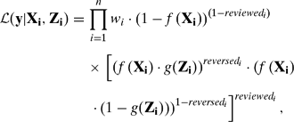
where wi is the weight (capturing over- or underrepresentation in the sample) for observation i. We programmed and maximized the log-likelihood in R.
One might also suppose that strategic whistleblowing by potential dissenting lower court judges may be correlated both with the lower court's ideological alignment with the Supreme Court and the Supreme Court's decision to review and/or reverse the lower court's decision (e.g., Hettinger, Lindquist, and Martinek Reference Hettinger, Lindquist and Martinek2004; Kastellec Reference Kastellec2007). Thus, we also estimated our empirical model including this control variable.Footnote 23
RESULTS
Our results are reported in Table 1. Notice first that the point estimates and variance for each of the parameters are essentially identical across the two specifications (with and without the dissent control). Because Model 2 is the best fit to the data (according to the AIC), we focus on it for our substantive interpretations. All of the substantive conclusions we draw, however, hold for both models.
Estimates from the Empirical Model

Notes: Estimates from maximizing the log of equation (1); point estimates with standard errors in parentheses; review parameters capture effect of covariates on the decision to review a case; reversal parameters capture effect of covariates on the decision to reverse a case once reviewed.
Our empirical analysis results are consistent with our theoretical predictions. Consider the review parameters (the β's). The negative estimate of β1 and the positive estimate of β2 indicate that the probability of review is a non-monotonic function of distancei; as expected, the probability of review initially decreases and then increases as the courts become more ideologically divergent. In fact, the substantive magnitude of this effect is considerable, as is demonstrated in the top-left panel in Figure 4. As a lower court becomes more ideologically divergent, the probability of review initially decreases, but then begins to increase. The bottom-left panel in Figure 4, moreover, shows the marginal effect of ideological distance on the probability of review. As predicted, the marginal effect of preference divergence changes from a negative effect at low levels of divergence to an increasingly positive effect at high levels of divergence. This differential effect of ideological distance on the probability of review is precisely what was predicted in Hypothesis 1.
Substantive Effect of Ideological Distance on Probability of Review and Reversal

Consider next our estimates of the reversal parameters (the γ's). Again, we find support for our hypothesis: The positive estimated coefficient associated with distancei and the negative estimated coefficient associated with distance2i together indicate a pattern whereby the probability of reversal initially increases as the courts become more divergent and then decreases. This relationship is shown in the top-right panel in Figure 4: The probability of reversing a decision that has been reviewed initially increases as the lower court becomes more divergent from about 40% to nearly 55%; however, as the lower court becomes increasingly distant, the probability of reversal drops to about 35%. The bottom-right panel shows the marginal effect of ideological divergence across the range of observed divergence. As predicted, the marginal effect of preference divergence changes from a positive effect at low levels of divergence to an increasingly negative effect at high levels of divergence. This empirical pattern comports with the expectation outlined in Hypothesis 2, providing additional support for the (counterintuitive) predictions derived from the theoretical model.
We briefly note in conclusion the estimates associated with our control variable. A nonunanimous lower court decision (one with a dissenting judge) is much more likely to be reviewed by the Supreme Court than a unanimous decision; the point estimates associated with this variable in the review part of the model are substantively very large. The predicted probability that a case from a lower court of average distance will be reviewed is 2% without a dissent, but 9% with a dissent. The presence of a dissent in the lower court has a comparable effect on the probability that the Supreme Court will reverse the lower court. In the absence of a dissent, the predicted probability that the Supreme Court will reverse a lower court decision is 52% (average distance, using estimates from Model 2). When there is a dissenting opinion, the predicted probability rises to 60%. This finding is largely in line with the literatures on certiorari and whistleblowing, which suggests an incentive for lower court judges to dissent in an effort to signal to the Supreme Court that it should hear the case (e.g., Beim and Kastellec Reference Beim and Kastellec2011; Caldeira, Wright, and Zorn Reference Caldeira, Wright and Zorn1999; Perry Reference Perry1991). However, as noted earlier, the inclusion of this control variable does not considerably change the estimated relationship between ideological alignment and the Supreme Court's decisions.
The implications of these empirical findings are considerable. As noted earlier, many of the standard tests used in the literature to assess whether the lower courts have strategic or myopic preferences cannot discriminate among various accounts of judicial behavior. In particular, by considering dispositions or rules alone, those studies risk missing important dynamics. Our theoretical model, by incorporating those dual considerations, reveals a series of discriminating predictions, and the analysis here reveals striking support for those hypotheses.
CONCLUSION
A major area of inquiry in the study of American politics concerns rule making in a hierarchical institution. Perhaps chief among the substantively compelling institutions are the courts. With the judicial hierarchy's broad powers for lawmaking, the ways in which it shapes or constrains judicial decisions have broad implications for understanding much of the law. As noted at the outset of this article, the courts of appeals are often the final voice on important legal questions. We have developed a model of Supreme Court-lower court interactions that goes beyond existing theory. By combining a theoretical analysis of rule creation with a bottom-up perspective on the judicial hierarchy, we have uncovered a variety of striking features about the way in which law is created by lower courts. Our analysis yields several equilibrium predictions about judicial behavior that intuition predicts should exist yet no previous theory can explain. For example, our model predicts that the Supreme Court will intentionally review and affirm lower courts to alter the legal rule used in their decisions. In addition, our model highlights several difficulties with previous empirical strategies used to assess compliance and strategic behavior in the judicial hierarchy. Moreover, several of the results and comparative statics that derive from our analysis run counter to modal perceptions and intuitions and lead naturally to new empirical tests that future research can and should contemplate.
An empirical analysis of two of the SCRM model's most striking predictions has yielded results consistent with two of its counterintuitive predictions. Specifically, we have shown that there is a non-monotonic relationship between ideological divergence and both the likelihood of review and the likelihood of reversal. As lower courts become more divergent, they become at first less likely to be reviewed and then more likely to be reviewed. In contrast, as lower courts become more divergent, they become first more likely, but then less likely, to be reversed. Although we investigated only a limited set of the model's predictions, the evidence is striking.
Nevertheless, there is work still to be done. The findings reported here are but one step forward. The results of this study can and should be incorporated into the broader literatures on the development of law (e.g., Kornhauser Reference Kornhauser1992; Lax Reference Lax2007), judicial compliance and top-down rule making (e.g., Cameron, Segal, and Songer Reference Cameron, Segal and Songer2000; Clark Reference Clark2009), and the structure of legal rules (e.g., Lax Reference Lax2009; Staton and Vanberg Reference Staton and Vanberg2008). The formal models we develop have broader implications for rule making in a hierarchy (e.g., other judicial hierarchies, administrative bureaucracies). Our results may be exported to those settings for further interpretation and empirical analysis. Short of that future research, our study yields a series of important lessons about the judicial hierarchy. Perhaps most important, the evidence reveals that strategic considerations by the lower courts lead to more complicated nuanced incentives and patterns of behavior than standard models would predict.
APPENDIX: PROOFS AND SUPPLEMENTAL RESULTS
Proof.Proof of Proposition 1. The following strategy profile constitutes the unique perfect Bayesian equilibrium to the model:

First notice that because UC's decision cannot affect LC's utility, it is always optimal for LC to select r = L. This gives LC the best possible rule and always results in LC's preferred disposition. Thus, ULC(r = L) = φ; this is the best possible utility for LC. It is optimal for UC to audit LC's decision only when UUC(audit) ≥ EUUC(¬audit). By the utility function defined earlier, USC(audit) = φ − k. UC's expected utility from not auditing depends on the rule selected by LC and whether the realized case facts and disposition implied by r correspond to UC's preferred disposition. When UC observes the rule r = L and the disposition “exclude” (E), then UC knows that f > L. Given f > L, UC prefers the disposition E. Thus, EUUC(¬audit|r = L, E) = φ − L 2. Thus, on observing E, UC prefers to audit only when k ≤ L 2. When UC observes r = L and the disposition “admit” (A), then UC's expected utility from not auditing depends on the realized case facts and the rule selected by LC. Specifically,  . Thus, on observing A, UC prefers to audit only when
 . ■
Proof.Proof of Proposition 2. Note, Proposition 2 characterizes a continuum of isomorphic equilibria where there are three cases. The cases are determined by a cutpoint in the fact-space, rA ∈ [r, r]. To characterize equilibrium behavior, we first establish a series of intermediate results.
Lemma 1.The Upper Court reviews a case whenever  .
Proof.UUC(review|r) = φ − k and EUUC(¬review|r) = −r 2 + bφ, where b is the Upper Court's beliefs over the probability that the Lower Court has declared a rule that yields the Upper Court's preferred disposition. The parameter b is a decreasing function of r; by Brouwer's fixed point theorem a solution to this equality exists. The Upper Court reviews a case whenever EUUC(review|r) > EUUC(¬review|r). ■
Corollary 1.If the Upper Court observes (r ≥ 0, Exclude), the Upper Court reviews if  and does not review if
 .
Proof. If the Upper Court observes (r ≥ 0, Exclude), b = 1 because the Upper Court always wants Exclude for any f > 0, and the Upper Court knows that f > r on observing (r ≥ 0, Exclude). The Upper Court is indifferent over changing the rule when it knows it is getting its preferred disposition when  . ■
Corollary 2.The Upper Court does not review if r ∈ [0, r for any b ∈ [0, 1], where  .
Proof. The Upper Court prefers not to review for b ≥ 0 if EUUC(review|r) = φ − k ≤ EUUC(¬review|r) = −r 2. ■
Lemma 2.The Lower Court never prefers to be reviewed.
Proof. This proof is constructed in three steps. First, the Lower Court never offers r < 0. If the Lower Court offers r = 0, the Upper Court never reviews (UUC(¬review|r = 0)= φ > UUC(review|r = 0)= φ − k). If the Lower Court offers r<0 and is reviewed, the Lower Court gets the same outcome as if it set r = 0. If the Lower Court offers r < 0 and is not reviewed, the Lower Court is strictly worse off. If f < r, ULC(r < 0|¬review) = −(r − L)2 + φ < ULC(r = 0|¬review) = −L 2 + φ. If f ∈ [r, 0], ULC(r < 0|¬review) = −(r − L)2 < ULC(r = 0|review) = −L 2 + φ.
Second, the Lower Court never offers r > L. If the Lower Court offers r = L and is not reviewed, the Lower Court gets its optimal outcome. If the Lower Court offers r = L and gets reviewed, the Lower Court is also reviewed for any r > L. Because  , and we know
 for r > 0, therefore EUUC is decreasing in r.
Because the Lower Court never has an incentive to offer a rule outside of the Pareto set, the Lower Court never prefers to be reviewed. If f < 0, ULC(¬review) = −(r − L)2 + φ > ULC(review) = −L 2 + φ. If f ∈ [0, L], ULC(¬review) = −(r − L)2 + φ or −(r − L)2. Either way, ULC(review) = −L 2 < ULC(¬review|f ∈ [0, L]). And if 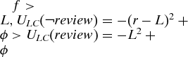 . ■
Corollary 3.By proof of Lemma 2, the Lower Court never makes an offer outside the Pareto set, r ∈ [0, L], for any b ∈ [0, 1].
Lemma 3.For  , the Lower Court's sequentially rational move is to offer
 .
Proof. Consider first f > L. By Corollary 1, the Upper Court reviews if and only if  . By Lemma 2, the Lower Court never prefers to be reviewed. The rule closest to the Lower Court's most preferred rule that will not be reviewed is
 . Consider next
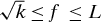 . By Corollary 1, the largest rule that the Upper Court will not review is
 . By Lemma 2, the Lower Court never prefers to be reviewed. Thus, a Lower Court with case facts
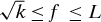 sets
 . ■
Lemma 4.All equilibria Footnote 24must involve pooling by Lower Courts with case facts f < 0 and the subset of Lower Courts with case facts 0 < f < rA over a rule in the set r ∈ [r, r], where  and
 .
Proof. If the Lower Court offers  , the Upper Court reviews by Lemma 1. By Corollary 2, the Upper Court never reviews any rule where 0 ≤ r ≤ r. Because the Lower Court never prefers to be reviewed (Lemma 2), and the Lower Court wants a rule as close to its ideal rule as possible, we know
 must hold.
Suppose ![$r^{\prime}\in (\underline{r},\sqrt{k}]$](https://static.cambridge.org/binary/version/id/urn:cambridge.org:id:binary:20160312035233457-0489:S000305541200024X_inline42.gif?pub-status=live) is offered by a Lower Court with case facts f < 0, and it separates from all Lower Courts with case facts 0 < f < L. The Upper Court does not review by Corollary 1. A Lower Court with case facts 0 < f < L strictly prefers to offer r = r′ over offering r ≤ r because r′ will not be reviewed. Further, if a Lower Court with case facts 0 < f < r chooses any other
![$r\in (\underline{r},\sqrt{k}]$](https://static.cambridge.org/binary/version/id/urn:cambridge.org:id:binary:20160312035233457-0489:S000305541200024X_inline43.gif?pub-status=live) in equilibrium, the Upper Court knows f > 0, b = 0, and by Lemma 1 the Upper Court reviews. Because by Lemma 2 any lower Court with case facts 0 < f ≤ r′ prefers to pool on r′ ratherthan be reviewed, we have a contradiction and separation is unsustainable.
Finally, because the equilibrium must entail pooling behavior, and the Upper Court cannot review the Lower Court with certainty on observing the equilibrium rule, r* (by Lemma 2, the Lower Courts with case facts  would deviate to
 ), the Upper Court at most must be indifferent over reviewing the rule. Because from above all Lower Courts with case facts f ≤ r′ will pool on r′, by Lemma 1 the Upper Court is indifferent over reviewing a rule when
 . Thus
 must hold. ■
Lemma 5.Given the possible equilibrium behavior defined in Lemma 4, the beliefs that can support this behavior are as follows. On equilibrium path, on observing  . Off equilibrium path, on observing (0 ≤ r < r*, Admit), b can cover the entire support. Off equilibrium path, on observing
 ,
 must hold.
Proof. For (r*, Admit), r* is on equilibrium path, and so beliefs must be updated by Bayes rule. Thus, 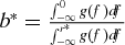 . For (0 ≤ r < r*, Admit), the Lower Court always prefers offering r* to any deviation to the left. Thus, Upper Court moves, and beliefs are unconstrained in this range. Finally, for
 , the Upper Court must prefer to review the rule in equilibrium, otherwise the Lower Court would deviate to r′. The Upper Court prefers to review whenever it believes the likelihood of a reversal on disposition is sufficiently high. By Lemma 1, this condition holds whenever
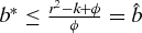 holds. ■
Lemma 6.For a Lower Court with case facts 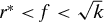 , the optimal r is the one closest to L for which the disposition is Exclude, r = f.
Proof. If a Lower Court with case facts 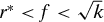 sets the rule greater than f, the disposition would be Admit. As proven in Lemma 5, on observing (r > r*, Admit) the Upper Court reviews and holds off equilibrium path beliefs
 . Thus, the Lower Court sets the rule at the largest value that would yield a disposition of Exclude and not be reviewed, r = f. ■
With these intermediate results established, we now demonstrate equilibrium behavior in each of the three cases. Formally, the equilibria characterized in Proposition 2 are given as follows:
![\begin{eqnarray*}
r^*(f)&=&\left\{
\begin{array}{@{}l@{}l@{}l@{}}
\sqrt{k}%\text{, Exclude}
&\text{if}&f>\sqrt{k}\\[6pt]
f\text%{, Exclude}
&\text{if}&f\in\left(r_a,\sqrt{k}\right]\\[6pt]
r_a%\text{, Admit}
&\text{if}&f\leq r_a
\end{array}
\right.\\
a^*(r)&=&\left\{
\begin{array}{@{}l@{}l@{}l@{}}
1&r\geq\sqrt{k}\\[6pt]
\left[0,1\right]&r\geq r_a&\text{and disposition is admit}\\[6pt]
0&\text{otherwise}
\end{array}
\right.
\end{eqnarray*}](https://static.cambridge.org/binary/version/id/urn:cambridge.org:id:binary:20160312035233457-0489:S000305541200024X_eqnU4.gif?pub-status=live)

where  is defined by Bayes rule and makes the Upper Court indifferent about auditing when r = ra.
Case 1 ( ): By Lemma 3,
 , which leads to the disposition Exclude. By Corollary 1, UC does not review the rule. To see that LC never has an incentive to deviate, consider first a deviation to any r′ < r*. For any beliefs and any move by UC, LC is strictly worse off. Consider next a deviation to any r″ > r*. By Corollary 1, UC reviews this rule. By Lemma 2, LC never prefers to be reviewed and therefore has no incentive to deviate to r″ > r*.
Case 2 ( ): By Lemma 4, LC picks r* = rA, which leads to the disposition Admit. By Lemma 5, on observing (r*, Admit),
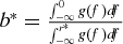 . By Lemma 4,
 and therefore UC does not review.
Suppose a deviation to r′ < r*. For any beliefs and any move by UC, LC is strictly worse off. Now, consider a deviation to r′ where L > r′ > r*. By Lemma 5,  , and UC reviews. By Lemma 2, LC never prefers to be reviewed. Therefore, there is no incentive to deviate. Finally, suppose a deviation to r″ > L. By Corollary 3, LC will never deviate to any r > L. UC's beliefs and moves are unconstrained.
Case 3 (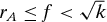 ): In this case, r* = f. r* = f gives a disposition of Exclude. r* = f, Exclude implies f ≥ r*, and therefore b = 1. By Lemma 6, LC has no incentive to deviate from r* in either direction. ■
Lemma 7.Given Proposition 2, if L ≥ r*(f), the behavior characterized by Proposition 2 holds in equilibrium; if L < r*(f), then the following strategy characterizes the Lower Court's strategy in all perfect Bayesian equilibria:
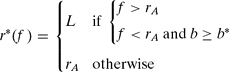
Proof. Suppose first L ≥ rA. Playing r* = L leads to a disposition of Exclude because, by assumption, L < r*(f). By Corollary 1, UC does not review. LC can do no better because it is choosing its optimal rule. Now, suppose L < rA. If on observing r < rA, b ≥ b*, then by Lemma 1, UC does not review. Again, LC is choosing its optimal rule and can do no better. Conversely, if on observing r < rA, b < b*, then by Lemma 1, UC does review. By Lemma 2, LC's best reply remains rA. ■
Proof.Proof of Proposition 3. Note, as in Proposition 2, we characterize a continuum of isomorphic equilibria, where there are multiple cases. To characterize equilibrium behavior in any one of these isomorphic equilibria, we first establish a series of intermediate results.
Lemma 8.The dominant strategies characterized by Lemmas 1 and 2, as well as their corollaries, continue to hold in this model by subscripting the k parameter with ki, i = l, h.
Proof. The Upper Court's objective function has not changed, except that the cost parameter, k is now subscripted by the Upper Court's type. Substituting in a subscripted k parameter does not alter the Upper Court's dominant strategies described by Lemma 1. ■
Lemma 9.All equilibria Footnote 25must involve pooling by Lower Courts with case facts f < 0 and the subset of Lower Courts with case facts 0 < f < rA over a rule in the set  .
Proof. Define 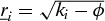 and
 , where i = l, h. If a Lower Court with case facts
 offers
 , the Upper Court always reviews (Lemma 1 and kl < kh). The Upper Court never reviews any rule where
 (Corollary 2, Lemma 8, and kl < kh). Because the Lower Court never prefers to be reviewed (Lemma 2 and 8) and the Lower Court wants a rule as close to its ideal rule as possible, we therefore know
 must hold. Whether
 or
 is the lower boundary on this range depends on whether
 holds. Substituting in for
 and
 , and solving for p yield
 .
Now, to see that only pooling behavior can be supported, assume that a Lower Court with case facts f ≤ 0 separates from all Lower Courts with case facts f ∈ (0, L). Now suppose first the Lower Court with case facts f ≤ 0 is playing  . A Lower Court with case facts 0 < f < r′ strictly prefers to offer r = r′ over offering
 because r′ will not be reviewed and the alternatives guarantee the Lower Court a worse rule and possibly a worse disposition as well. If a Lower Court with case facts f ∈ (0, r′] offers any other
 the Upper Court knows f > 0, b = 0, and by Lemmas 1 and 8 either type of Upper Court reviews. Because the Lower Court never prefers to be reviewed (Lemmas 2 and 8), we have a contradiction.
Suppose, on the other hand, that the Lower Court with case facts f ≤ 0 is playing ![$r^{\prime}\in (\overline{r}_l, \overline{r}_h]$](https://static.cambridge.org/binary/version/id/urn:cambridge.org:id:binary:20160312035233457-0489:S000305541200024X_inline81.gif?pub-status=live) . A Lower Court with case facts 0 < f < r′ strictly prefers to offer r = r′ over offering r ≤ rh because
 and
 must hold (otherwise the Lower Court with case facts f ≤ 0 would deviate and play rl or rh as well). If a Lower Court with case facts f ∈ (0, r′] offers any other
 , the Upper Court knows f > 0, b = 0, and by Lemmas 1 and 8 either type of Upper Court reviews. Because the Lower Court never prefers to be reviewed (Lemmas 2 and 8), we once again have a contradiction. ■
Definition 1. Let  .
Lemma 10.Given the possible equilibrium behavior defined in Lemma 9, beliefs that can support this behavior are as follows. On equilibrium path, on observing 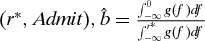 . If
 , on observing the off-equilibrium path play (0 ≤ r′ < r*, Admit), b can cover the entire support. If
![$r^{*}\in (\overline{r}_l, \overline{r}_h]$](https://static.cambridge.org/binary/version/id/urn:cambridge.org:id:binary:20160312035233457-0489:S000305541200024X_inline88.gif?pub-status=live) , on observing the off-equilibrium path play (0 ≤ r′ < r*, Admit), b can cover
 . Off equilibrium path, on observing
 , b can cover
 .
Proof. For (r*, Admit), r* is on equilibrium path, and so beliefs must be updated by Bayes rule. When  , for (0 ≤ r′ < r*, Admit) the Lower Court always prefers offering r* to any deviation to the left. Thus, Upper Court moves, and beliefs are unconstrained in this range. When
![$r^{*}\in (\overline{r}_l, \overline{r}_h]$](https://static.cambridge.org/binary/version/id/urn:cambridge.org:id:binary:20160312035233457-0489:S000305541200024X_inline93.gif?pub-status=live) , for (0 ≤ r′ < r*, Admit) the Lower Court prefers r* to any deviation to the left as long as an Upper Court with ki = kl prefers to review the deviation. By Lemmas 1 and 8, this condition holds when
 holds. Finally, for
 , the Upper Court with ki = kh must prefer to review the rule in equilibrium, otherwise the Lower Court would deviate to r′. The Upper Court prefers to review whenever it believes the likelihood of a reversal on disposition is sufficiently high. By Lemmas 1 and 8, this condition holds whenever
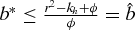 holds. Note that the beliefs described here are sufficient, but not necessarily necessary for the behavior in Lemma 9 to be sequentially rational. ■
Lemma 11.There are multiple types of equilibria that may exist, but we focus on those where courts with f < 0 always pool on a single r. (a) When there are multiple  , the Lower Court always prefers to choose the largest. (b) When there are multiple
 , the Lower Court always prefers to choose the largest. (c) There may be a case where
 . This, however, is a knife-edge condition. (d) We rule out arbitrary mappings from model parameters to rules.
Lemma 12.For a Lower Court with case facts  , where i = l if
 and i = h; otherwise, the optimal r is the largest one for which the disposition is Exclude, r = f.
Proof. If a Lower Court with case facts  sets the rule greater than f, the disposition would be Admit. As proven in Lemma 10, on observing (r′ > rA, Admit), the Upper Court reviews and holds off-equilibrium path beliefs
 . Thus, the Lower Court sets the rule at the largest value that would yield a disposition of Exclude and not be reviewed, r = f. ■
Lemma 13.A Lower Court with case facts  sets
 if
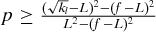 and r = f otherwise.
Proof. By Corollary 1, the Upper Court reviews if and only if  . Thus, if the Lower Court offers
 , the Lower Court receives −(l − r)2. If the Lower Court offers
 , the Upper Court reviews iff k = kl, and the Lower Court receives −pL 2−(1 − p)(L − r)2. Thus, the Lower Court sets the rule closest to its most preferred rule that ensures neither type of Upper Court reviews the case (
 ) when
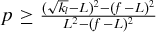 , and r = f otherwise. By Lemmas 2 and 8, the Lower Court never prefers to choose a rule that is reviewed with certainty, so no other behavior obtains. ■
Lemma 14.A Lower Court with case facts  sets
 where i = l if
 and i = h otherwise.
Proof. This proof is the same as Lemma 13, except for the fact that the Lower Court gets reviewed with certainty for any  , and so the best risky proposal the Lower Court can make is
 . ■
Lemma 15.For f > L, the Lower Court's sequentially rational move is to offer  where i = l if
 and i = h otherwise.
Proof. By Corollary 1, the Upper Court reviews if and only if  . By Lemmas 2 and 8, the Lower Court never prefers to be reviewed when k is known. Thus, the Lower Court either sets the rule closest to its most preferred rule that ensures neither type of Upper Court reviews the case (
 ) or that only the Upper Court with low costs, kl, reviews the case (
 ). The Lower Court offers
 when
 . Solving for p yields
 . ■
With these intermediate results established, we demonstrate equilibrium behavior. The following characterizes all pure-strategy perfect Bayesian equilibria to the model.
The Lower Court's equilibrium strategy is given by
![\begin{eqnarray*}
r^*(f;p\le \hat{p})&=&\left\lbrace \begin{array}{@{}l@{}l@{}l@{}}r_{a_h}\in \left[\underline{r_l},\overline{r_h}\right]\text{, Admit}&\text{if}&f\le r_{a_h}\\[6pt]
f\text{, Exclude}&\text{if}&f\in \left(r_{a_h},\sqrt{r_h}\right]\\[6pt]
\sqrt{k_h}\text{, Exclude}&\text{if}&f>\sqrt{k_h} \end{array} \right.\\[6pt]
r^*(f;p>\hat{p})&=&\left\lbrace \begin{array}{@{}l@{}l@{}l@{}}r_{a_l}\in \left[\underline{r_l},\overline{r_l}\right]\text{, Admit}&\text{if}&f\le r_{a_l}.\\[6pt]
f\text{, Exclude}&\text{if}&f\in \left(r_{a_l},\sqrt{r_l}\right]{\!}.\\[6pt]
\sqrt{k_l}\text{, Exclude}&\text{if}&f>\sqrt{k_l} \end{array} \right.
\end{eqnarray*}](https://static.cambridge.org/binary/version/id/urn:cambridge.org:id:binary-alt:20160626053319-76479-mediumThumb-S000305541200024X_eqnU7.jpg?pub-status=live)
The Upper Court's equilibrium strategy is given by
![{\fontsize{8}{10}\selectfont{\begin{eqnarray*}
a^*(r; i=l)&=&\left\lbrace \begin{array}{@{}l@{}l@{}l@{}}
1&\text{if}\left\lbrace \begin{array}{@{}l@{}l@{}l@{}}
r\ge \sqrt{k_l}\\[6pt]
r\in \left(r_{a_l},\sqrt{k_l}\right]\text{and disposition is Admit}\\[6pt]
r\in \left(\overline{r}_l,\overline{r}_h\right]\text{and disposition is Admit} \end{array}\right.\\[26pt]
\left[0,1\right]&\text{if}r\in \left(\underline{r}_l,r_{a_l}\right)\\[6pt]
0&\text{otherwise} . \end{array} \right. \\[6pt]
a^*(r; i=h)&=&\left\lbrace \begin{array}{@{}l@{}l@{}l@{}}
1&\text{if}\left\lbrace \begin{array}{@{}l@{}l@{}}
r\ge \sqrt{k_h}\\[6pt]
r\in \left(r_{a_h},\sqrt{k_h}\right]\text{and disposition is Admit} \end{array}\right.\\[16pt]
\left[0,1\right]&r\in \left(\underline{r}_l,r_{a_h}\right)\\[6pt]
0&\text{otherwise} \end{array} \right.
\end{eqnarray*}}}](https://static.cambridge.org/binary/version/id/urn:cambridge.org:id:binary-alt:20160626053324-13166-mediumThumb-S000305541200024X_eqnU8.jpg?pub-status=live)
The Upper Court's beliefs are given by

where  is defined by Bayes’ rule and makes the Upper Court with type i indifferent about auditing when
 .
Now, consider five cases. Case 1 ( ): By Lemma 9, the Lower Court pools on
 if
 , which leads to a disposition of Admit. If, however,
 , the Lower Court pools on
 , which leads to a disposition of Admit. By Lemmas 1 and 8, the Upper Court reviews if i = l and
![$r_{A_h}\in (\overline{r}_l,\overline{r}_h]$](https://static.cambridge.org/binary/version/id/urn:cambridge.org:id:binary:20160312035233457-0489:S000305541200024X_inline132.gif?pub-status=live) . The Upper Court's beliefs are given by Lemma 10.
Case 2 ( ): By Lemma 9, the Lower Court pools on
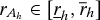 if
 , leading to a disposition of Admit. However, if
 , then by Lemma 12 the Lower Court plays a separating strategy and plays r = f, leading to a disposition of Exclude. By Lemmas 1 and 8, the Upper Court reviews if i = l and the Lower Court plays
![$r_{A_h}\in (\overline{r}_l,\overline{r}_h]$](https://static.cambridge.org/binary/version/id/urn:cambridge.org:id:binary:20160312035233457-0489:S000305541200024X_inline137.gif?pub-status=live) . In the event the Lower Court plays the pooling strategy, and the Upper Court's beliefs are given by Lemma 10. When the Lower Court plays a separating strategy, then the Upper Court believes it has received its preferred disposition with certainty, because any r > 0 and Exclude implies f > 0.
Case 3 ( ): By Lemma 12, the Lower Court plays a separating strategy and plays r = f, leading to a disposition of Exclude. By Lemmas 1 and 8, the Upper Court does not review. Observing r > 0 and Exclude implies f > 0, so b = 1.
Case 4 ( ): By Lemma 13, the Lower Court will play
 if
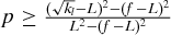 . Otherwise, the Lower Court will continue to play its separating strategy and offer r = f. Both strategies lead to a disposition of Exclude. By Lemmas 1 and 8, the Upper Court does not review
 if i = l, but will review a rule
 if i = l. By Lemmas 1 and 8, the Upper Court reviews neither rule if i = h. In any case, observing r > 0 and Exclude implies f > 0, which implies b = 1.
Case 5 ( ): By Lemma 15, the Lower Court offers
 if
 and
 otherwise. Any of these rules leads to a disposition of Exclude. By Lemmas 1 and 8, the Upper Court does not review either rule if i = h and reviews any rule
 if i = l. Observing r > 0 and Exclude implies f > 0, which implies b = 1. ■
Lemma 16.Given Proposition 3, if L ≥ r*(f; p), the behavior characterized by Proposition 3 holds in equilibrium; if L < r*(f; p), then the following strategy characterizes the Lower Court's strategy in all perfect Bayesian equilibria:

Proof. The proof follows immediately from the proof of Lemma 7 demonstrated above. ■
 and
 is arbitrary. Specifically,
 whenever
 . Because b can vary arbitrarily (for example, as a function of g(·)), the specific ordering can vary arbitrarily.
 all increase.
 , and
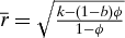 . For k sufficiently small, (e.g., k<1 for
 .
 or where the Lower Court is indifferent between playing a risk-averse and a risk-seeking strategy. For the latter knife-edge condition, this possibility introduces no new observable behavior, because the Lower Court would simply be choosing among already identified equilibrium strategies.
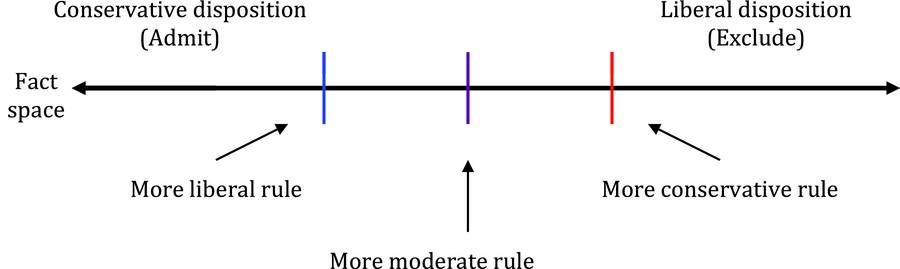
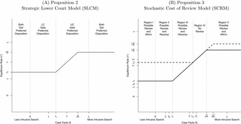
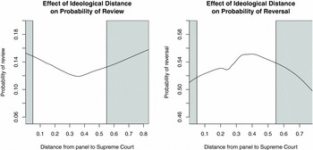
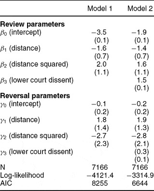
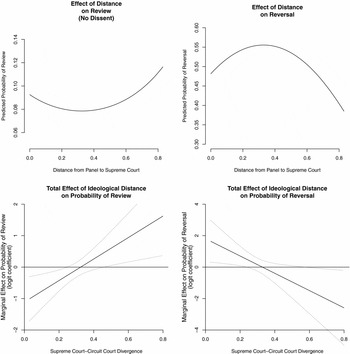



Comments
No Comments have been published for this article.