1. Introduction
Cavitation poses a design concern for liquid-operated devices as per guidelines imposed by international authorities (IMO, 2014), impacting performance by increasing drag in hydronautical vehicles, limiting propulsion system thrust, inducing large-scale underwater radiated noise (URN) (Sezen et al. Reference Sezen, Dogancan, Refik, Osman and Mehmet2021), reducing turbine power output and efficiency, and affecting the pump head and efficiency. This hydrodynamic phenomenon, typically characterised by bubble clusters or clouds, occurs in liquids with significant pressure gradients involving multiple scales in time and space (Arakeri et al. Reference Arakeri and Acosta1973). Cavitation can manifest in different forms (such as bubbles, sheets, clouds and vortexed cavities) (Franc & Michel Reference Franc and Michel2004). The specific appearance is contingent on factors such as flow velocity, fluid quality (presence of dissolved air nuclei) and the geometry of the body involved (Ahn et al. Reference Ahn, Jeong, Park and Kim2020). Cavitation around a hydrofoil encompasses a spectrum of intricate dynamic phenomena, including mass transfer through phase change and diffusion, occurrence of shockwaves, and both large- and small-scale instabilities and turbulence (Smith et al. Reference Smith, Venning, Pearce, Young and Brandner2020). The instability of cavity shedding defines the unstable nature of partially cavitating flows (Franc Reference Franc2001). Understanding this unstable nature is fundamental for understanding this topic. Callenaere et al. (Reference Callenaere, Frank, Michele and Riondet2001) categorised the instabilities of an attached cavity into intrinsic and system instabilities, emphasising the role of the re-entrant jet in inducing unstable oscillating cavity shedding through a simple description of the development of a re-entrant jet in an adverse pressure gradient. As the partial cavity grows and expands towards the trailing edge, an adverse pressure gradient zone at the closure of the sheet cavity causes the re-entrant jet to shift from primary instability, which drives shedding to shockwave instability (Kjeldsen, Arndt Roger & Effertz Reference Kjeldsen, Arndt Roger and Effertz2000). The re-entrant jet advances upstream, breaking up the cavity surface and forming a detached cloud cavity contingent upon closure in a region with a significant adverse pressure gradient and sufficient thickness to limit the re-entrant jet–cavity interface interaction. Periodic cloud shedding and shock propagation are recognised as the primary contributors to instabilities and discrete noise peaks.
Under specific conditions, multiple instabilities may coexist, featuring both bubbly shock propagation and re-entrant jet flow detaching from the sheet cavity, leading to cloud shedding (Ganesh, Simo & Ceccio Reference Ganesh, Simo and Ceccio2016). Venning et al. (Reference Venning, Khoo, Pearce and Brandner2018) explained complex multi-stage shedding cycles involving both re-entrant jet and shockwave instabilities. Shockwave formation and propagation depend on the bubble density and the coherent collapse of bubbles owing to interactions within the detached cloud cavity. Various studies based on Reynolds’s initial investigation have aimed to enhance our understanding of cavitation phenomena by exploring aspects such as cavitation vapour formation (Kadivar et al. Reference Kadivar, Thanh-Hoang, Warn-Gyu and Ould2021), bubble detachment dynamics (Blake & Gibson Reference Blake and Gibson1981), boundary layer behaviour (Franc & Michel Reference Franc and Michel1985), and recent efforts to control or mitigate cavitation strength, extent, dynamics and impact (Kadivar et al. Reference Kadivar, Timoshevskiy, Nichik, Ould, Schellin and Pervunin2020). Cavitation control through flow-control methods refers to instruments used to modify the inherent characteristics of fluid flows, steering them towards controlled and preferred conditions. These approaches can be broadly categorised into passive (Hilo et al. Reference Hilo, Hong, Ahn, Paik, Jeong, Kim and Kim2023) and active (Hilo et al. Reference Hilo, Kim, Hong and Ahn2025) strategies. Passive solutions involve devices that operate independently without requiring external controllers or energy sources, distinguishing them from actively controlled methods (Zaresharif et al. Reference Zaresharif, Florent, David and Yan M.C.2021). Fruman et al. (Reference Fruman, Dugué, Pauchet, Cerrutti and Briançon-Marjollet1992) and Fruman, Cerrutti & Pichon (Reference Fruman, Cerrutti and Pichon1995) investigated cavitation and vortex dynamics on hydrofoils with geometries similar to those used in our experiments. Their studies highlighted the sensitivity of viscous flows to leading-edge roughness and Reynolds number scaling, providing critical insights into boundary layer development, vortex roll-up and tip vortex cavitation phenomena.
Hence, the primary goal of this study is to assess the efficacy of protuberances for passive cavitation control experimentally. This involves examining cavitation-related parameters, including the cavitation inception number, cavity shedding volume, cavitation structural characteristics and sound pressure level (SPL) in the frequency domain, to suppress cavitation and minimise flow-induced noise. This study explores the physics characterising diverse cavitation regimes around hydrofoils mimicking biological structures featuring leading-edge (L-E) protuberances with varying geometrical parameters within a cavitation tunnel. This study employs high-speed imaging, synchronised force measurements and noise signal measurements. Furthermore, this investigation emphasises the importance of structural characteristics, sheet cavitation periodicity and subsequent cloud cavity shedding, both with and without L-E protuberances. Increasing the Reynolds number on the cavitation intensity and flow-induced noise production are also considered. A combination of high-speed pressure transducers is used for the assessment. Notable reductions in the cavitation and noise are observed under specific operating conditions. Moreover, the conditions for the initial occurrence of noticeable cavitation (cavitation inception), including the cavitation number and Reynolds number, are identified. Comparative analyses among the modified hydrofoils are conducted to discern the specific roles of the amplitude and wavelength in the L-E sinusoidal geometries.
2. Background
Biomechanics and functional morphology harness engineering principles to elucidate the intricate relationships between anatomical structures and their functions. Unravelling flight mechanics requires understanding steady and unsteady aerodynamics, whether in avian or insect species. Similarly, understanding the swimming behaviour of aquatic living creatures entails applying the principles of hydrodynamics. This interdisciplinary approach, guided by physics and technology, has enhanced our understanding of biological forms and functions. A continual focal point for hydrodynamic experts is enhancing performance and efficiency in engineering applications by mimicking the flow control mechanisms of aquatic animals and striving to improve hydrodynamic models across diverse contexts (Fish & Lauder Reference Fish and Lauder2006). Incorporating L-E protuberances or sinusoidal wavy structures observed in whale flippers minimises noise and enhances both hydrodynamic and aerodynamic performance (Watts & Fish Reference Watts and Fish2001). Extensive research has established that introducing such protuberances or sinusoidal structures at the L-E of hydrofoils can enhance their hydrodynamic performance, particularly under post-stall conditions and the overall operating envelope of the angle of attack. In a numerical study, Watts and Fish (Reference Watts and Fish2001) used panel methods to simulate the airflow over a wing profile (NACA 634-021), comparing conditions with and without modified L-E protuberances at an angle of attack of 10 and 4.8 % gain in the lift over the baseline wing, and a 10.9 % decrease was observed. Miklosovic et al. (Reference Miklosovic, Murray, Howle and Fish2004) demonstrated that incorporating tubercles resulted in a delayed stall onset to a higher angle by approximately 40 %, accompanied by increased maximum lift, reduced drag and significantly expanded operating envelope. Therefore, the lift coefficient is comparatively lower at pre-stall angles and the modified hydrofoils exhibit improved performance at post-stall angles (Cai et al. 2015).
L-E modifications have been studied across various marine applications, including tidal turbines (Shi et al. Reference Shi, Rosli, Atlar, Norman, Wang and Yang2016), marine propeller blades (Stark, Shi & Troll Reference Stark, Shi and Troll2021) and rudders (Weber, Howle & Murray Reference Weber, Howle and Murray2010), revealing improved lift/drag performance and an expanded operating envelope (Zhao et al. Reference Zhao, Xu, Tang, Zhang, Zhao, Liu and Wei2021).
Various hypotheses have emerged regarding the flow control mechanism of L-E protuberances. While the prevailing theory suggests a similarity to the flow-control mechanisms of vortex generators (Wei, New & Cui Reference Wei, New and Cui2015), alternative studies suggest that the mechanism differs and behaves more akin to a stall strip rather than vortex generators (Seyhan, Sarioglu & Akansu Reference Seyhan, Sarioglu and Akansu2021). Our previous research (Simanto et al. Reference Simanto, Hong, Kim, Ahn Ahn and Shin2022) explored the hydrodynamic performance and cavitation effects of the protuberance functionality as a passive flow control technique on several NACA0012 two-dimensional (2-D) hydrofoils. As a progression from our previous work on 2-D hydrofoils, this study delves into more realistic scenarios involving three-dimensional (3-D) elliptical hydrofoils. This advancement seeks to comprehend the intricate 3-D flow over hydrofoils with L-E protuberances, addressing a research gap in which prior studies have primarily focused on hydrodynamic performance, neglecting cavitation effects and protuberance functionality as passive flow-control techniques.
3. Experimental and numerical methods
3.1. Experimental facility and technique
Measurements were conducted using a variable-pressure high-speed cavitation tunnel at Chungnam National University in the Flow-Induced Noise and Cavitation Control Laboratory (FINCL). The specifications of Chungnam National University Cavitation Tunnel (CNUCT) are detailed in figure 1. The tunnel test section measures 100 square mm by 1000 mm long, enabling the variation of operating velocity and absolute pressure within the ranges of approximately 120 ms−1 and 10–300 kPa, respectively. The contraction ratio was 15 : 1, and the flow speed was calculated with an error of less than 0.1 % using an LDV and absolute pressure sensors (ETM-200–375M, USA). The transparent acrylic walls of the cavitation tunnel enable optical access to capture images of the flow field. The flow characteristics were documented using high-speed cameras capable of capturing the flow field at up to 8 00 000 fps. The cameras were equipped with a maximum shutter speed of 2 μs and a CMOS sensor detected light signals within the field of view. A Gigabit Ethernet cable facilitated the connection between the cameras and the computer. Light-emitting diode (LED) lamps provided illumination for the field of view with a luminous flux of 12 500 lm (150 W).
Simple schematic view of Chungnam National University Cavitation Tunnel (CNUCT).

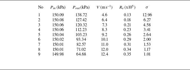
Measurements were conducted at wide ranges of various angles of attack (AOA), at 4°, 8°, 12°, 16° and 20°. Furthermore, chord-based Reynolds numbers (R
e
= U
∞
C/ν) ranged between 0.13 × 10⁵ and 0.34 × 10⁵, where C is the mean chord (m), U
∞ is the free stream velocity (m s–1) and ν is the kinematic viscosity of the water (m2 s–1). The cavitation number (σ), defined as σ = (p
∞
−
 $p_{v}$
)/0.5ρU
∞
2, where p
∞
is the absolute static pressure (Pa),
 $p_{v}$
is the vapour pressure (Pa) and ρ is the water density (kg m–3), was systematically adjusted from 12.96 to 1.17 to explore different cavitation regimes. The sound pressure level was obtained through experimental methods. A pair of XTM-190M (Kulite) pressure transducers were used for this purpose. These transducers were flush mounted on the observation window, with one positioned at 0.5C and the other at 1.5C along the axis of rotation, where C represents the chord length of the hydrofoil. The pressure fluctuation data recorded by the transducers were subsequently converted into frequency-domain data through a Fourier transform. This technique allowed for evaluating both quasi-steady and unstable cavitation oscillation frequencies, providing insight into the acoustic characteristics associated with cavitation. The recorded pressure fluctuation data were then converted into frequency-domain data, enabling the evaluation of both the quasi-steady and unstable cavitation oscillation frequencies. In addition, the noise levels generated during the partial cavity creation and collapse processes were quantified in terms of the SPL for each hydrofoil model and plotted against the Strouhal number (S
t
). Strouhal number (S
t
) is expressed as S
t
= (f C / U
∞
) (here, f represented the noise frequency).
Table 1 provides the specifications of the equipment used in the experimental set-up, detailing the instruments and their operational parameters. Throughout all the measurements, dissolved oxygen levels were maintained within the range of 6–8 ppm. A degassing system was incorporated in the CNUCT to regulate the air nuclei content, effectively ensuring the expulsion of air bubbles from the inflow of the circulating liquid to control the air nuclei. The utility of this system has been demonstrated in previously published studies, particularly in the context of ventilated supercavitation and the effectiveness of bubbly flows. Table 2 outlines the test conditions and experimental parameters, carefully selected based on pre-test evaluations to ensure alignment with the study’s objectives.
Equipment specifications of the experimental set-up.

Test conditions and experiment parameters.

Model hydrofoils (baseline and with L-E modifications) were attached to three-component load cells with an estimated precision of 0.1 %, along with data acquisition software to measure the hydrodynamic forces. The model was secured to the load cell using six fixing bolts, each featuring a radial clearance of 0.5 mm between the load cell and test-section wall to prevent interference with force measurement. Figure 2 shows the configuration of the load cell, depicting how the models are positioned within it and how the angle of attack is measured concerning the rotation point.
Hydrofoil model assembly on load cell and angle of attack. (a) Hydrodynamics force measurement loadcell. (b) Angle of attack (AOA) in the x–z plane. (c) Angle of attack (AOA) in the x–y plane.

3.2. Experimental uncertainty
A comprehensive uncertainty analysis was conducted to ensure the experimental findings’ reliability, precision and reproducibility. Recognising the importance of addressing potential sources of error, we systematically evaluate the accuracy of the instruments, calibration methods and data collection processes. The study aims to provide confidence in the experimental results and minimise ambiguity by thoroughly validating measurements through repeatability tests and cross-verifications. Velocity measurements were conducted using laser Doppler velocimetry (LDV) positioned at the tunnel inlet, where cavitation and bubbles were absent. To verify the accuracy, the LDV readings were compared with velocities derived from pressure differences, demonstrating excellent agreement (e.g. LDV measured 9.2 m s–1, while calculated velocities from absolute pressure transducers ranged between 9.10 and 9.12 m s–1). Data collection commenced only after stable readings were achieved from both methods. The LDV uncertainty, specified as 0.067 % by the manufacturer, was calibrated to ensure precision in velocity measurements.
The uncertainty in SPL measurements was analysed using pressure fluctuations recorded by a pair of XTM-190M (Kulite) pressure transducers, which were flush-mounted on the observation window at 0.5C and 1.5C along the hydrofoil’s axis of rotation. The recorded pressure fluctuation data were converted into the frequency domain using a Fourier transform, and the resulting spectral peaks were validated against the periodic cloud shedding observed during cavitation tests on a NACA 0012 hydrofoil across various cavitation numbers. This validation process aligns with the findings in figure 13 of Ahn et al. (Reference Ahn, Jeong, Park and Kim2020). To ensure accuracy, we calibrated the transducers to confirm the absence of pressure fluctuations in the tunnel when no obstacles were present, thus minimising external sources of uncertainty.
The performance of the 3-component force transducer was evaluated to ensure its accuracy and reliability in measuring forces (F x , F y ) and moment (M z ). Load tests were conducted across a range of applied loads, from 0 to 30 kg for F x and F y , and up to 3 kg m for M z . The force measurements demonstrated minimal variations during increasing and decreasing load cycles, confirming high precision. Similarly, the moment measurements exhibited high linearity and negligible deviations, ensuring consistent performance for torque measurement.
Key performance metrics, including linearity, hysteresis and repeatability, were analysed to validate the transducer’s reliability. The output exhibited a strong linear relationship, with deviations of −0.02 % for F x and 0.15 % of full scale (F.S.) for F y . Negligible hysteresis effects were observed between loading and unloading cycles, confirming the absence of measurement memory effects. The transducer also showed excellent repeatability, with variations remaining within 0.05 % of F.S. across repeated measurements, highlighting its reliability under consistent load conditions.
The transducer’s capacity and output sensitivity were verified for compatibility with the experimental set-up. The measurement range was confirmed as ±30 kg for F x and F y , and ±3 kg m for M z , with output sensitivities of 0.4155, 0.4119 and 1.2653 mV V–1, respectively. Input/output resistances of 350 Ω (F x and F y ) and 700 Ω (M z ) further validated the system’s robustness and compatibility with instrumentation. These evaluations demonstrate the transducer’s ability to provide precise, repeatable and reliable measurements, meeting the stringent requirements of the experimental study.
3.3. Designing of L-E protuberances
This study focused on four NACA 16020 profile 3-D elliptical hydrofoil models consisting of one baseline and three modified models at the L-E (depicted in figure 3). Each model had a chord length of 60 mm and a span length of 60 mm, deliberately selected to examine the impact of L-E tubercles on cavitation, hydrodynamic performance, and noise emission arising from solid–fluid interaction and cavitation propagation. Previous experimental and numerical studies predominantly explored the capability and applicability of L-E protuberances under cavitating conditions using rectangular hydrofoils.
Test models from different views: (a) Baseline, (b) W06S, (c) W12S, (d) W12AS, (e) bottom view, ( f) top view.

The credibility of this investigation technique for rectangular hydrofoils has been established in various contexts, aligning with applications involving wing sections and allowing the examination of flow on 2-D rectangular hydrofoils to avoid the complexities associated with integrated 3-D flow. However, when extending passive control using LE modification to other aquatic applications such as propulsion or water turbine blades, relying solely on investigations with 2-D rectangular foils becomes inadequate for accurately predicting applicability. With this consideration in mind and to explore more realistic scenarios, our experimental investigation used elliptical hydrofoil models. These models, characterised by 3-D multiphase flow under the applied conditions, offer a more comprehensive understanding of the effectiveness of the concept in diverse hydrodynamic environments.
Designing of L-E protuberances on elliptical hydrofoils: (a) W06S; (b) W12S; (c) W12AS.

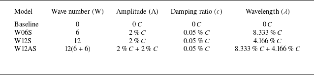
The amplitude (A) and wavelength (λ) constitute the primary criteria for LE modification with a sinusoidal protuberance on rectangular hydrofoils. As elucidated in previous studies (Custodio, Henoch & Johari Reference Custodio, Henoch and Johari2018; Simanto et al. Reference Simanto, Hong, Kim, Ahn Ahn and Shin2022), the performance of the modified hydrofoils varies significantly based on these two parameters. In this study, A and λ are also regarded as significant design parameters. Given that the models in this investigation are elliptical, damping (ε) is applied to the sinusoidal wave to ensure the smoothness of the design (design concepts are illustrated in figure 4). The LE geometry of all modified models is defined by (4), along with the wavenumber (W), amplitude (A) and wavelength (λ), as listed in table 3.
Specification of the test models.

 \begin{align} Y_{\textit{LE}\left(W06S\right)} &=A_{1}\, e^{-\varepsilon j}\sin \left(\frac{180j}{\lambda _{1}S}\right), \end{align}
 \begin{align} Y_{\textit{LE}\left(W12S\right)} &=A_{2}\, e^{-\varepsilon j}\sin \left(\frac{180j}{\lambda _{2}S}\right), \end{align}
 \begin{align} Y_{\textit{LE}\left(W12AS\right)} =Y_{\textit{LE}\left(W06S\right)}+Y_{\textit{LE}\left(W12S\right)}. \end{align}
The Y
LE
values for the `W06S’ model have been determined by solving (3.1), substituting the values of wavelength (λ
1) as 8.333 % C, amplitude (A) as 2 % C and damping
 $\varepsilon \, =$
0.05 % C. Here, C, S and W were set to 60 mm, 60 mm and 6, respectively, and j is the position concerning the y-axis. To obtain the Y
LE
values for the L-E of the ‘W12S’ model from (3.2), λ
2
was adjusted to 4.166 % of C. To calculate the appropriate value for λ, W was altered to 12 while keeping the other values the same as in the ‘W06S’ model.
In addition to implementing two symmetric modifications to the L-E, we introduce a more realistic third design. This approach, reminiscent of prior aerodynamic studies (Demirci, Seyhan & Sarioglu Reference Demirci, Seyhan and Sarioglu2023), aligns with the experimental inspiration drawn from humpback whale flippers. The asymmetrical sinusoidal tubercles on humpback whale flippers served as a model for the third design. The Y LE values for the ‘W12AS’ model were derived by solving (3.3), a summation of Y LE values from (3.1) and (3.2). This process results in an asymmetrical design along the L-E, encompassing two distinct wavelengths and amplitudes.
3.4. Numerical method
Large eddy simulation (LES) was employed in this numerical study to solve the governing equations, as it is well suited for capturing the complex interactions between turbulence and cavitation. Versteeg and Malalasekera (Reference Versteeg and And Malalasekera2007) noted that LES applies a spatial filtering operation to distinguish between large and small eddies in turbulent flow. This approach directly resolves large-scale coherent structures, while the effects of small-scale structures are modelled using a sub-grid-scale (SGS) model.
LES has been widely recognised for its high fidelity in capturing critical flow phenomena such as cavity growth, collapse and re-entrant jet behaviours, making it particularly effective for complex geometries like hydrofoils. Previous very recently published studies (Liu et al. Reference Liu, Wei, Cao and Wan2023; Wang et al. Reference Wang, Liu, Li, Wang, Huang and Wu2024; Mou et al. Reference Mou, Che, Zhang, Wang, Cao and Wu2024; Chen et al. Reference Chen, Guo, Zhang, Wang, Liu, Wu and Hu2024) have demonstrated the capability of LES to predict the physical characteristics of cavitating flow around hydrofoils accurately. This includes the resolution of coherent turbulent structures and cavity-shedding behaviours. In contrast, conventional turbulence models such as Reynolds-Averaged Navier–Stokes (RANS) often struggle to capture turbulence–cavitation interactions effectively. RANS models are particularly inadequate in resolving features within regions of strong unsteadiness, such as those downstream of the leading-edge protuberance. For this reason, LES was chosen as the primary turbulence model in this study to ensure accurate predictions of the cavitating flow behaviour and its interaction with hydrofoil geometries.
3.4.1. Governing equations
By applying a filtering function, we obtain the following LES continuity and momentum equations:
 \begin{align} \frac{\partial \rho _{m}}{\partial t} + \frac{\partial }{\partial x_{i}}\left(\rho _{m}\bar{u}_{i}\right)& =0, \end{align}
 \begin{align} \frac{\partial }{\partial t}\left(\rho _{m}\bar{u}_{i}\right)+\frac{\partial }{\partial x_{j}}\left(\rho _{m}\bar{u}_{i}\bar{u}_{j}\right)& =-\frac{\partial \bar{P}}{\partial x_{i}} \frac{\partial }{\partial x_{j}}\left({\rm \mu} _{m}\frac{\partial \bar{u}_{i}}{\partial x_{j}}\right)-\frac{\partial \tau _{ij}}{\partial x_{j}}+\rho _{m}g, \end{align}
where
 $\bar{u}$
and
 $\bar{P}$
represent the filtered velocity and pressure field, respectively, and
 $\bar{\tau }_{ij}$
represents the SGS stress. The SGS stress is defined as follows:
 \begin{equation} \bar{\tau }_{ij}=\rho _{m}(\overline{u_{i}u_{j}}-\overline{u_{i}}\overline{u_{j}}). \end{equation}
Furthermore, the SGS stress is modelled using the Smagorinsky–Lilly model, in which the local stresses are assumed to be proportional to the local strain rate tensor (
 $\bar{S}_{ij})$
,
 \begin{equation} \bar{\tau }_{ij}=-2{\rm \mu} _{\textit{SGS}}\bar{S}_{ij}+\frac{1}{3}\tau _{ij}\delta _{ij}=-{\rm \mu} _{\textit{SGS}}\left(\frac{\partial \bar{u}_{i}}{\partial x_{j}}+\frac{\partial \bar{u}_{j}}{\partial x_{i}}\right)+\frac{1}{3}\tau _{ij}\delta _{ij}, \end{equation}
where
 ${\rm \mu}_{\textit{SGS}}$
represents the SGS viscosity and is evaluated by (3.8). In this equation, C
SGS
is constant and C
SGS
= 0.1, as Versteeg & Malalasekera (Reference Versteeg and And Malalasekera2007) recommended. Additionally,
 $\varDelta_{s}$
is the mixing length of the SGS model and is defined as (3.10), where V, K and C
W
represent the volume of the grid cell, the von Kármán constant and the WALE model parameter, respectively. In this study, the WALE model parameter (C
W
= 0.544) was selected (Zhi et al. Reference Zhi, Huang, Qiu, Wang and Huang2022).
 \begin{align} {\rm \mu} _{\textit{SGS}}& =\rho \left(C_{\textit{SGS}}\varDelta _{s}\right)^{2}|\bar{S}| =\rho \left(C_{\textit{SGS}}\varDelta _{s}\right)^{2}\sqrt{2\bar{S}_{ij}\bar{S}_{ij}}, \end{align}
 \begin{align} \bar{S}_{ij}& =\frac{1}{2}\left(\frac{\partial \bar{u}_{i}}{\partial x_{j}}+\frac{\partial \bar{u}_{j}}{\partial x_{i}}\right), \end{align}
 \begin{align} \varDelta _{s}& =\min \left(\mathrm{K }_{d},C_{W}V^{\frac{1}{3}}\right). \end{align}
Cavitation model. In the numerical calculations, the Schnerr–Sauer cavitation model (Schnerr & Sauer Reference Schnerr and Sauer2001) was applied to simulate the phase change from water to vapour. The governing equation for vapour is as follows:
 \begin{align} & \frac{\partial \alpha _{v}}{\partial t}+\frac{\partial \left(\alpha _{v}u_{i}\right)}{\partial x_{i}}=\frac{1}{\rho _{v}}\left( \dot{m}^{+}-\dot{m}^{-}\right), \end{align}
 \begin{align} & \dot{m}^{+}=\alpha _{v}\left(1-\alpha _{v}\right)\frac{\rho _{w}\rho _{v}}{\rho _{m}}\frac{3}{R_{b}}\sqrt{\frac{2}{3}\frac{\left(p_{v}-p\right)}{\rho _{w}}} ,\quad p\leq p_{v}, \end{align}
 \begin{align} & \dot{m}^{-}=\alpha _{v}\left(1-\alpha _{v}\right)\frac{\rho _{w}\rho _{v}}{\rho _{m}}\frac{3}{R_{b}}\sqrt{\frac{2}{3}\frac{\left(p-p_{v}\right)}{\rho _{w}}},\quad p\geq p_{v}, \end{align}
 \begin{align} & \;R_{b}=\left(\frac{\alpha _{v}}{1-\alpha _{v}}\frac{3}{4\pi }\frac{1}{N_{b}}\right)^{\frac{1}{3}}, \end{align}
where
 $\dot{m}^{+}$
and
 $\dot{m}^{-}$
are the mass transfer rates owing to evaporation and condensation, respectively. Here,
 $\alpha _{v}$
, N
b
and R
b
are the volume fraction of the vapour, the nuclei density per volume of liquid water and the bubble diameter, respectively.
3.4.2. Computational set-up and validation
A computational domain was designed based on the experimental conditions for the numerical calculations. A hydrofoil with a chord length of 60 mm at the root was positioned at the centre of the calculation domain. Figure 5 illustrates the three-dimensional computational domain, highlighting the boundary conditions, hydrofoil placement and domain dimensions. The calculation domain had dimensions of 1.67C, 1.67C and 18C, corresponding to the height, width and length, respectively. The inlet was placed 8C upstream and the outlet was located 10C downstream of the centre of the root chord. Uniform free-stream velocity and static pressure were applied at the inlet and outlet, respectively, as the boundary conditions. A no-slip wall condition was set for both the hydrofoil surface and the computational walls.
Three-dimensional representation of the computational domain, showing boundary conditions, hydrofoil placement and domain dimensions.

(a) Computational mesh, (b) non-dimensional v-velocity field (x = 1C), (c) grid convergence test for v-velocity component (y = 0); the experiment was reported by Nagarathinam et al. (Reference Nagarathinam, Hong, Ahn, Park, Kim and Moon2022).

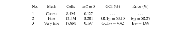
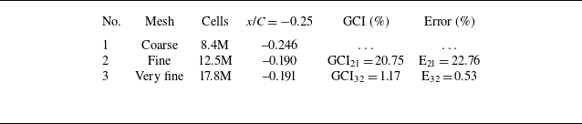
During the simulations, a hexahedral mesh was generated using the STAR-CCM + hexahedral mesh generator, as shown in figure 6(a). To satisfy the requirements of the wall-resolved LES (y+ ≈ 1), a prism layer with 30 layers and a total thickness of 0.5 mm was applied to refine the mesh on the hydrofoil surface. In addition, a tip vortex refinement region was defined to investigate the tip vortex cavitation more accurately. Three meshes were created for comparison: a coarse mesh (8.4 million cells), a fine mesh (12.5 million cells) and a very fine mesh (17.8 million cells). A grid-independence test was conducted for the baseline hydrofoil test model under fixed flow conditions (U ∞ = 8 m s–1, AOA = 10°). Figure 6(b) illustrates a non-dimensional y-velocity field at a location x = 1C downstream of the hydrofoil in the case of the fine mesh.
Tables 4 and 5 present the results of the mesh independence test for v/U∞. Table 4 corresponds to x/C = 0, while table 5 corresponds to x/C = −0.25. These tables provide a clear comparison of the results, demonstrating the mesh-independent behaviour of the solution and ensuring the reliability of the computational analysis.
Mesh independent test for
 $v$
/U
∞ at x/C = 0.

Mesh independent test for v/U ∞ at x/C = −0.25.

Figure 6(c) shows that the numerical results for the v-velocity component for the three grids considered were consistent. The maximum error between the coarse and fine meshes was 16.88 %, whereas that between the fine and very fine meshes was 4.31 %. Considering both the accuracy and computational cost, a fine mesh was selected as the final mesh for all numerical calculations.
To verify the accuracy of the numerical code, we first compared the numerical results with experimental data reported in the previously published work by Nagarathinam et al. (Reference Nagarathinam, Hong, Ahn, Park, Kim and Moon2022). As shown in figure 6(c), the numerical results for the v-velocity component are in good agreement with the experimental data. We then conducted numerical simulations for the four test models: Baseline, W06S, W12S and W12AS. The test models are described in § 3.3. As shown in figure 7, under the same flow conditions as the current experiment (R e = 0.31 × 10⁵, AOA = 12°, σ = 1.17), the numerical results are consistent with the experiment for all considered test models, including cloud cavitation on the hydrofoil’s surface and tip vortex cavitation. Comparisons of the numerical results with previously published works and current experiments show that the numerical simulations accurately predicted the cavitating flow over the hydrofoil.
Comparison of numerical and experimental results (R
e
= 0.31 × 10⁵, AOA = 12°). For the numerical results, the cavity boundaries are defined as the isosurface of vapour volume fraction of 10 % (α
 ${}_{v}$
= 0.1).

4. Results and discussion
4.1. Shedding mechanism and compartmentalisation of cavitation
It has been theorised that LE tubercles employ a flow-control mechanism involving compartmentalisation akin to the functionality observed in fences mounted on aircraft wings. In a numerical investigation, Cai et al. (Reference Cai, Zhou, Liu, Zuo, Zhang and Li2022) detailed the augmentation of hydrodynamic performance and provided compelling evidence supporting the compartmentalisation mechanism attributed to LE tubercles. This theory was also evident in our previous study on rectangular hydrofoils with LE protuberances in 2-D scenarios. The significance of compartmentalisation in cavitation control by LE tubercles has been emphasised, with previous discussions focusing on delaying stalls through flow attachments and detachments on alternate troughs. This study provides insights into how the exact mechanism compartmentalises a cavitating flow, effectively dividing a large sheet cavity into smaller cavity pockets. To understand the formation of cavity pockets as a whole, the flow from each cycle of the protuberance (peak-trough-peak) must be explained. The counter-rotating vortex from each peak towards the trough has been mentioned in previous literature, where the counter-rotating vortex forces the incoming flow towards the trough and the velocity increases; thus, the pressure decreases in the trough, creating pressure differences in the peaks and troughs, confining the flow primarily towards the trough, and restricting the expansion in the spanwise direction. As protuberances introduce a cyclic distribution of circulation in the spanwise direction, following Stokes’ law for spanwise circulation, the spanwise vorticity is expected to vary along the span of the hydrofoil. Each protuberance unit can be considered analogous to a small, finite and spanwise section. Similar to the generation of counter-rotating tip vortices in the streamwise direction, the cyclic variation in spanwise circulation governs the formation of pairs of counter-rotating streamwise vortices. The curl of the velocity vector results in the development of vorticity, which is influenced by the velocity and pressure differences from the peak downstream towards the valley (the development process is illustrated in figure 8). As the cavity incepted and propagated chordwise, the compartmentalisation effect became evident, resulting in cavity pockets.
Flow control mechanism (flow compartmentalisation) of the sinusoidal protuberance.

The compartmentalisation effect induced by LE tubercles significantly alters the shedding dynamics of cavitating flows. Unlike the baseline hydrofoil, which exhibits large, coherent cloud shedding with substantial force fluctuations and unsteady cavitation dynamics, the hydrofoil with LE tubercles breaks these structures into smaller, localised shedding events. This behaviour is directly linked to the compartmentalised cavity pockets formed by the counter-rotating vortices generated within each peak-trough-peak cycle of the tubercles. These vortices confine the flow within specific regions, restricting the spanwise expansion of cavitation structures and promoting a more controlled shedding process.
By disrupting large-scale cloud shedding, the LE tubercles effectively reduce the intensity and scale of shedding events, leading to diminished force fluctuations and a more stable cavitation regime. This study’s phase-averaged flow visualisations and comparative analysis highlight the differences in shedding dynamics between hydrofoils with and without LE tubercles, underscoring the role of tubercles in stabilising cavitating flows. This compartmentalisation mechanism demonstrates the ability of LE tubercles to modulate cavitation behaviour, making them a critical design element in mitigating unsteady cavitation-induced effects.
The experiments were conducted under different flow conditions and at various AOAs ranging from 8° to 20°, explaining the various flow characteristics. As the Reynolds number increases (R e ), the cavitation number (σ) decreases beyond the point of inception and the hydrofoil exhibits various cavitation forms. This encompasses the formation of partial sheet cavities followed by cloud shedding and extends to the occurrence of supercavitation. In addition, if the vorticity attains sufficient strength, leading to a pressure decrease at the core below the vapour pressure, vortex cavitation (VC) may also occur.
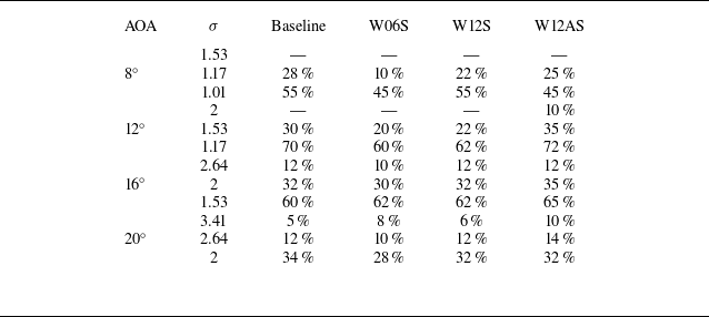
In this study, the investigation focused on a 3-D multiphase flow over elliptical hydrofoils, indicating that all the aforementioned cavitation types are likely to be present under specific conditions. This comprehensive analysis aims to evaluate the influence of a passive control technique, specifically the application of LE protuberances with various geometrical shapes, on various types of cavitation. The primary focus was examining partial cavities, specifically those covering approximately 55 %–65 % of the chord length, as exceeding this range may lead to supercavitation at certain AOAs. The shape and length of these partial cavitations varied with the AOAs. Table 6 presents the experimental measurements of cavity length as a percentage of the chord length for different cavitation numbers (σ) and AOA. The data were derived by averaging instantaneous images of the cavity to capture the extent of cavitation on the hydrofoil surface accurately. The observed variation in cavity length across repeated measurements is within the range of ±0.5 % ∼ 2 %. The results reveal that hydrofoils with leading-edge protuberances (W06S, W12S and W12AS) generally exhibit shorter cavity lengths than the baseline hydrofoil, particularly at lower σ, indicating their effectiveness in reducing cavitation extent. This reduction is more pronounced in configurations with sharper or asymmetrical protuberances, suggesting enhanced control of cavitation dynamics. These findings are crucial for understanding the influence of tubercles on cavitation behaviour under different flow regimes and provide a reliable dataset for comparison with computational analyses, thereby emphasising the potential of leading-edge protuberances in mitigating cavitation effects and improving flow stability. Visualisation data and detailed explanations are provided in § 4.2, which showcases different cavitation numbers while maintaining similar shapes and severities to conduct a thorough analysis of the partial cavities. For example, at an AOA of 8°, the severity and shape of the sheet cavity at σ = 1.01 resembled those at σ = 1.17 for AOA = 12°, and similar cavity formation was observed at 16° and 20° even at higher cavitation numbers.
Averaged cavity length measurements for various angles of attack.

4.2. Numerical results and discussion
As demonstrated by the experimental results, the protuberances on the L-E of a hydrofoil have significant effects on both the cavitating flow and the hydrodynamic characteristics. However, owing to limitations in the experimental conditions, understanding the physical mechanisms underlying the effects of protuberances on cavitating flows remains challenging. Numerical results were considered and investigated at both qualitative and quantitative levels to address this gap. First, as shown in figure 7, under fixed flow conditions (R e = 0.31 × 10⁵, AOA = 12°, σ = 1.17), the protuberances located on the L-E of modified hydrofoils induce the separation of the sheet cavity on the hydrofoil surface. These structures divide the cavity into smaller pockets, with the size of each pocket depending on both the number and height of the protuberances. The numerical results are in good agreement with the experimental results.
Comparisons of the SGS turbulent kinetic energy with instantaneous isosurfaces of Q criterion (Q = 1.000.000 s−2) at a physical time (t 0 to t 0 + 50 ms): (a) Baseline; (b) W06S; (c) W12S; (d) W12AS.

To gain a deeper understanding of the physical mechanisms underlying the effects of protuberances on the formation of the sheet cavity on the hydrofoil, a comparison of the SGS turbulent kinetic energy for the baseline hydrofoil model and other modified hydrofoils is presented in figure 8. This analysis depicted the SGS turbulent kinetic energy using instantaneous isosurfaces of the Q criterion (Q = 1.000.000 s–2) at a fixed physical time (t = 0.15 s). It is worth noting that in LES, the SGS turbulent kinetic energy represents the kinetic energy of unresolved turbulent motions at scales smaller than the grid size. This energy is crucial in LES models because it characterises the energy contained in the unresolved turbulent fluctuations. As depicted in figure 9, the SGS turbulent kinetic energy around the LE region increased with an increase in the number of protuberances. Furthermore, based on the numerical results, the modified hydrofoil model (W12AS) with asymmetric protuberances appeared to induce the highest turbulent kinetic energy compared with the baseline model and the other two modified hydrofoils. To validate this observation, the SGS turbulent kinetic energy at a location of chord length (x = –0.33C) among the considered test models was quantitatively compared in figure 9.
The numerical results in figures 9 and 10 show that hydrofoils with protuberances on the L-E led to an increased turbulent kinetic energy compared with the base hydrofoil. The physical mechanism underlying this finding can be attributed to the following factors. First, the protuberances at the L-E can disrupt the smooth flow of water over the hydrofoil surface, causing the boundary layer to become turbulent. This disturbance increases mixing within the boundary layer, resulting in higher turbulent kinetic energy. Second, the presence of protuberances can trigger the formation of vortices along the hydrofoil surface. These vortices can induce further turbulence in the flow, thereby contributing to higher TKE levels of turbulent kinetic energy. In summary, hydrofoils with protuberances on the L-E introduce disturbances that disrupt the flow, leading to an increased turbulent kinetic energy compared with a base hydrofoil. This phenomenon has implications for the performance and efficiency of hydrofoils in various applications.
Comparisons of SGS turbulent kinetic energy on a location of chord length (x = −0.33C): (a) Baseline; (b) W06S; (c) W12S; (d) W12AS.

Figure 11 shows the streamwise vorticity on the suction side of the considered hydrofoils at different chord locations. Under fixed flow conditions (R e = 0.31 × 10⁵, AOA = 12°, σ = 1.17), the streamwise vorticity distribution varies significantly between the baseline model and the other modified hydrofoils. In particular, a positive vorticity was observed on the L-E of the baseline hydrofoil, as shown in figure 11 (a). However, because of the effects of the protuberance structure, the streamwise vorticity along the L-E was distributed into clockwise and counterclockwise vorticities for all modified hydrofoils (W06S, W12S and W12AS), as depicted in figure 11(b–d). This result was consistent with the numerical observations reported by Pena et al. (Reference Pena, Muk-Pavic, Thomas and Fitzsimmons2019). The numerical results are shown in figures 11 and 12, providing clear evidence of the effects of the protuberance structure on the formation of vortices along the surface of the hydrofoils.
Streamwise vorticity on the surface and at different chord locations: (a) Baseline; (b) W06S; (c) W12S; (d) W12AS.

Comparison of streamwise vorticities at the L-E: (a) Baseline; (b) W06S; (c) W12S; (d) W12AS.

Cavitation pattern with and without LE protuberances at AOA = 8°, σ = 1.53–1.01: (a) Baseline; (b) W06S; (c) W12S; (d)W12AS.

Vortices generated by protuberance structures can help control the separation of the boundary-layer flow. Separation can be induced and controlled by strategically placing these structures, which is beneficial for managing the flow around the hydrofoils. In addition, vortices can increase lift generation on the hydrofoil surface. By energising the flow and preventing premature separation, these vortices contribute to higher lift coefficients, potentially leading to improved hydrofoil performance.
4.3. Cavitation pattern and acoustic performance at AOA = 8°
Under the carefully selected test conditions and evaluation parameters listed in table 2, AOA at 8°, 12°, 16° and 20° was selected for visualisation, ensuring meticulous consideration of the cavitation number criteria to capture cavitating flow propagation within the targeted range of 45 %–55 % of the chord length for each fixed AOA. At 8°, a minimal cavity manifested at σ = 1.53, whereas the partial cavity length expanded to the desired extent at σ = 1.01. Cavitating flow patterns at σ = 1.17 were observed between these two extremes. Figure 13 provides instantaneous images from high-speed videos, providing a comprehensive view of the flow dynamics at these three critical σ values. At σ = 1.53, the curl near the tip lacked sufficient strength to capture continuous tip vortex cavitation (TVC) within a single instantaneous image. No cavity was generated near the L-E for the baseline, W06S or W12S model. However, in the case of W12AS, cavity inception was observed near the trough of LE protuberances with large amplitudes. At σ = 1.17, the inflow velocity increased and the pressure on the suction side decreased. Hence, the vorticity near the tip increased due to the difference in pressure between the pressure and suction sides. Therefore, TVC can be observed on each model. As shown in figure 13, under σ = 1.17, the baseline foil exhibited a full-span partial sheet cavity, extending approximately 25 %–30 % chordwise with oscillating cloud shedding.
Sound pressure level with and without LE protuberances at AOA = 8°: (a) σ = 1.53; (b) σ = 1.17; (c) σ = 1.01.

Cavitation pattern with and without LE protuberances at AOA = 12°, σ = 2.00–1.17: (a) Baseline; (b) W06S; (c) W12S; (d) W12AS.

In contrast, the LE-modified models with protuberances exhibited a distinctive spanwise cavity pattern, effectively fragmenting the large sheet cavity into smaller pockets. This observed phenomenon is attributed to the compartmentalisation effect discussed earlier. Moreover, a similar trend was observed as the sheet cavity expanded to almost 50 % chordwise at σ = 1.01. Under this flow condition, the large cloud shedding from the baseline is divided into smaller bubble clouds and the large hairpin vortices can be observed in smaller sizes.
Compartmentalisation can be observed for the W06S and W12S models; however, the flow becomes more turbulent because of its asymmetrical LE shape and the cavity pockets are spanwise. Figure 14(a–c) presents the acoustic performance analysis, showcasing SPL (dB) against Strouhal’s number (S t ) at σ = 1.53, σ = 1.17 and σ = 1.01 in panels (a), (b) and (c), respectively. The acoustic emissions from hydrofoils with and without protuberances exhibited similar outputs at this specific AOA. The SPL showed no significant decrease or increase for the hydrofoils with protuberances compared with the baseline hydrofoil at this particular AOA. However, it is essential to highlight that the variations in noise levels became more pronounced at higher AOAs. This phenomenon is explored and discussed in detail in the subsequent sections of this study.
4.4. Cavitation pattern and acoustic performance at AOA = 12°
To assess the cavitation pattern with a comparable partial cavity shape, covering nearly 50 % of the chord length, instantaneous images at σ = 2.00–1.17 are shown in figure 15 for the Baseline, W06SS, W12S and W12AS and are denoted as (a), (b), (c) and (d), respectively. Cavity fragmentation is evident in all modified hydrofoils across various cavitating conditions in the range of 10 %–20 % of the chord (at σ = 1.53) to exceed 50 % of the chord (at σ = 1.01), where the partial sheet cavity is prominent. Findings from the acoustic analysis at this AOA align with our previous approach (Simanto et al. Reference Simanto, Hong, Kim, Ahn Ahn and Shin2022) of evaluating the acoustic performance of LE protuberances. As the cavitation number (σ) decreased, the effectiveness of LE protuberances in controlling noise emissions became more prominent.
Sound pressure level with and without LE protuberances at AOA = 12°: (a) σ = 2.00; (b) σ = 1.53; (c) σ = 1.17.

When the cavity on the suction side intensified, the re-entrant jet intersected the large sheet, causing a subsequent burst of significant cloud shedding. This results in a shockwave interacting with the flow and solid surface, contributing to an overall increase in sound pressure. Because of the compartmentalisation effect, hydrofoils with LE and LE protuberances exhibit reduced shockwave amplitudes and lower SPLs, even under conditions of severe cavitation, as smaller cloud shedding results in low-intensity shockwaves. Figure 16(a) shows that the highest noise level was observed for W12AS. The increased turbulence at the L-E, which is attributed to the LE geometry of this model, led to cavitation in the valley of each protuberance. At σ = 1.53, the cavitating flow over W12AS exhibited heightened severity compared with other models, resulting in elevated noise levels (figure 16 b). In addition, the noise levels for other modified models were marginally higher than the baseline hydrofoil, considering that the cloud cavity was not the predominant noise source at this stage. However, as the severity of the sheet cavity increased at σ = 1.17, accompanied by substantial cloud shedding, the noise level control exerted by the modified hydrofoil became distinctly apparent (figure 16 c). At this stage, the average SPL from W12S decreased by nearly 10 % (12–15 dB) compared with the baseline hydrofoil, with W6S and W12AS also exhibiting lower noise emissions than the baseline.
4.5. Cavitation pattern and acoustic performance at AOA = 16°
At higher AOAs, the cavitating flow revealed a distinct pattern compared with the lower and moderate AOAs. Tip vortex cavitation (TVC) at moderate AOAs strengthened as σ decreased. However, at a higher AOA, specifically, AOA = 16°, TVC weakened or almost dissipated with the increased flow velocity. This is because, at higher AOAs, the curl induced by the pressure difference between the sides of the hydrofoil is distributed over a wider area along the upper edge of the foil, extending beyond the tip area. As a result, the vortex becomes larger; however, the core loses strength, hindering the formation of an attached TVC. From the cavitating flow visualisation and SPL demonstrated in figures 17 and 18, respectively, a periodic fluctuation can be observed for all hydrofoils (baseline and modified); this fluctuation is because of the attachment and detachment owing to the re-entrant flow caused by the adverse pressure.
Cavitation pattern with and without LE protuberances at AOA = 16°, σ = 2.64–1.53: (a) Baseline; (b) W06S; (c) W12S; (d) W12AS.

Sound pressure level with and without LE protuberances at AOA = 16°: (a) σ = 2.64; (b) σ = 2.00; (c) σ = 1.53.

Cavitation along the L-E was evident within the initial 10 % chordwise at σ = 2.64. Compartmentalisation was noticeable (figure 17), revealing different cavity patterns on modified hydrofoils, and discerning differences in the sound pressure level (SPL) measurements between the baseline and modified hydrofoils were limited (figure 18 a). As the sheet cavity at σ = 2.00 extended chordwise, covering nearly 30 % of the chord length, fluctuations intensified in the flow dynamics and SPL. Notably, the SPL for the W12S model was lower than that of the baseline and other modified models, owing to the fragmentation into small cavity pockets. However, the W12AS model, despite sharing the same wave number, exhibited higher noise levels than the W12S model, which is attributed to more severe flow conditions arising from the presence of two different wavelengths among neighbouring protuberances.
As σ decreased to 1.53, the sheet cavity extended to approximately 50 %–60 % of the chordwise for all models. The extensive cloud shedding induced a shockwave that propagated on the baseline hydrofoil model, increasing the overall noise level. In contrast, the hydrofoils with LE protuberances exhibited lower SPLs. This reduction can be attributed to the compartmentalisation effect, where the large sheet cavity is divided into smaller pockets and the substantial cloud shedding is fragmented into smaller components. Consequently, this fragmentation results in an overall decrease in the noise level emitted by hydrofoils with LE protuberances.
4.6. Cavitation pattern and acoustic performance at AOA = 20°
At an extreme AOA = 20°, the cavitation pattern exhibited high fluctuations, indicative of the complex flow dynamics. Remarkably, despite extensive experimentation, no instances of TVC have been observed within the experimental range of flow conditions, underscoring the intricacies of cavitation phenomena under extreme operating conditions. The findings from instantaneous images captured by the high-speed video of the cavitating flow, as presented in figure 19, offer compelling insights into the transient nature of the cavitation behaviour across all models, including the baseline configuration.
Cavitation pattern with and without LE protuberances at AOA = 20°, σ = 3.41–2.00: (a) Baseline; (b) W06S; (c) W12S; (d) W12AS.

Notably, the visualisations underscored the significant instability in the cavitating flow regime, highlighting the challenges associated with controlling cavitation-induced effects in hydrodynamic systems. Furthermore, at high flow velocities (σ = 2.00), the occurrence of flow separation at approximately 30 %–40 % chordwise is noteworthy. This phenomenon significantly impacts the extension of the sheet cavity, resulting in an increased frequency of cloud shedding and further complicating the flow dynamics. Analysis of the SPL presented in figure 20(a,b,c) revealed that, despite significant fluctuations, there were no differences in SPL for hydrofoils with protuberances compared with the baseline hydrofoil at this specific AOA. This observation suggests that the presence of LE protuberances did not significantly influence the noise emission characteristics under the investigated flow conditions and AOA. However, while SPL measurements did not exhibit discernible variations between the baseline and modified hydrofoils, the underlying flow dynamics and noise generation mechanisms may differ.
Sound pressure level with and without LE protuberances at AOA = 20°: (a) σ = 3.41; (b) σ = 2.64; (c) σ = 2.00.

4.7. Hydrodynamic performance
Force measurements were systematically performed using a 3-component load cell to analyse the baseline and modified hydrofoil models, each featuring LE protuberances. The experiments covered a range of flow conditions and an AOA range of 4°–20°. The dimensionless parameters C L (lift coefficient) and C D (drag coefficient) used for assessing the hydrodynamic performance were derived from the force measurements of the lift and drag using (3.15) and (3.16), respectively, where F L represents the lift force, F D represents the drag force and A is the area of each model,
 \begin{align} C_{L}& =\frac{F_{L}}{\frac{1}{2}\rho AU^{2}},\end{align}
 \begin{align} C_{D}& =\frac{F_{D}}{\frac{1}{2}\rho AU^{2}}. \end{align}
Hydrodynamic performance evaluations were performed under varying conditions, encompassing both cavitating and non-cavitating states with a σ range of 3.41–1.53. Figures 21–24 depict the lift coefficient (C L ) and drag coefficient (C D ) on the y-axis concerning the AOA on the x-axis. At σ = 3.41, the lift demonstrated a linear increase as AOA varied from 4° to 16°, followed by a subtle decline at 20°. To enhance clarity in the hydrodynamic performance comparison, the notation 5C L and 5C D has been used for C L and C D by scaling their magnitudes by a factor of 5. Additionally, error bars have been added to figures 21, 22, 23 and 24 to represent the uncertainty in the measured loads, with adjustments made to align with the scaled values. This anticipated pattern aligned with the absence of partial cavities across all models up to 16°. However, at 20°, cavitation was apparent, leading to a reduced C L . This decrease can be attributed to the emergence of a spanwise cavity within 5 % of the chord, coupled with flow separation occurring near the mid-chord at the higher AOA. Despite increased C D at high AOAs for models with protuberances, the baseline hydrofoil and the modified models exhibited a similar trend.
Hydrodynamic performance comparison of the lift coefficient (C L ) and drag coefficient (C D ) in the y-axis and AOA in the x-axis of all hydrofoils at σ = 3.41.

Hydrodynamic performance comparison of the lift coefficient (C L ) and drag coefficient (C D ) in the y-axis and AOA in the x-axis of all hydrofoils at σ = 2.64.

Hydrodynamic performance comparison of the lift coefficient (C L ) and drag coefficient (C D ) in the y-axis and AOA in the x-axis of all hydrofoils at σ = 2.00.

Hydrodynamic performance comparison of the lift coefficient (C L ) and drag coefficient (C D ) in the y-axis and AOA in the x-axis of all hydrofoils at σ = 1.53.

At lower AOAs ranging from 4° to 8°, the baseline hydrofoil surpassed all its modified counterparts regarding lift-generating performance.
As the cavitation number decreased to σ = 2.64 (figure 22), the discernible influence of cavitation on lift production became increasingly pronounced. At this stage, various cavitation forms (TVC and partial sheet cavity) manifest and propagate over the hydrofoils, primarily at higher AOAs exceeding 12°. As a result, a significant decline (∼25 %) in the maximum C L was observed for all models at AOA settings of 16° and 20°. This was because of the prevalence of cavitation effects, as the partial cavity covers almost 10 %–15 % chordwise. Among the test models, W12AS generated a higher lift in all ranges of AOAs, particularly within the moderate to higher AOA range of 12°–20° (except the initial low angle). While W06S did not exhibit any significant performance difference compared to the baseline, overall, W12S generated the lowest lift.
A further deduction in C L is evident at higher AOAs (16° and 20°) when the cavitation number is reduced to σ = 2.00 since the sheet cavity covers approximately 25 %–35 % of the suction side chordwise. Even under this severe cavitating condition, the lift generation performance of W12AS outperformed the baseline model, whereas W06S also generated a slightly higher lift than the baseline. W12S remained the lowest lift-generating model. At higher AOAs (16° and 20°), pronounced fluctuations were apparent, stemming from the flow dynamics over the hydrofoil at these elevated AOAs. They occurred intermittently under high flow velocity, separation and reattachment, contributing to the observed fluctuations.
This behaviour intensified at a higher severity when σ = 1.53 for 16° and 20°. Although force measurement was feasible for 16°, the high-vibration conditions hindered accurate force measurement at 20°. Consequently, the results for AOA = 20° at this velocity were excluded from the analysis. Under this condition, W12AS performed better than other models, similar to the trend observed for C L . Furthermore, C D demonstrated significantly narrow distinguishable differences between models, showing a consistent trend identical to previous cavitating conditions.
5. Conclusion
In this study, we thoroughly explored the flow characteristics of elliptical hydrofoils across diverse flow conditions and a broad spectrum of angles of attack (AOAs). Our focus encompassed one baseline model and three LE bio-inspired modifications. We probed the hydrodynamic forces, noise emissions and ramifications of cavitation through meticulous experimental analyses. Furthermore, we employed numerical simulations to scrutinise the turbulent kinetic energy (TKE) and the occurrence of counter-rotating vortex phenomena. The integrity of our numerical findings was ensured through rigorous validation of both past and present experimental data, thereby enhancing the credibility of the results. After conducting investigations across various case scenarios, the following conclusions were drawn after summarising the key findings.
-
(i) Incorporating LE protuberances inspired by humpback whale flippers into modifying elliptical hydrofoil-induced compartmentalisation effects. This design feature effectively restricts the expansion of large sheet cavities and confines them to smaller cavity pockets.
-
(ii) Turbulent kinetic energy (TKE) analysis revealed a heightened energy flow between the peaks of each protuberance in the L-E modified models. This observation suggests that LE protuberances contribute to an enhanced turbulent kinetic energy, leading to a delay in flow separation. These findings imply an improved hydrodynamic performance for hydrofoils with LE protuberances.
-
(iii) Observing a counter-rotating vortex pair moving from the two peaks towards the adjacent trough highlights the modified hydrofoil’s heightened flow intensity in the trough area. In contrast, no counter-rotating vortices were detected in the baseline model under identical flow conditions and AOAs.
-
(iv) The sound pressure level (SPL) investigation revealed heightened efficacy in noise control mechanisms under elevated partial cavitation severity conditions. The interval between 12° and 16° AOA, where the cavity covers approximately half of the chord, is particularly noteworthy. In this range, the impact of LE modifications on the SPL reduction was most prominent, with the W12S model demonstrating the highest effectiveness. These findings underscore the significance of the LE protuberances in mitigating noise levels under specific hydrodynamic conditions.
-
(v) The hydrodynamic force analysis highlighted the positive impact of bio-inspired hydrofoil modifications on enhancing the lift coefficient and optimising the overall hydrodynamic performance. Specifically, the lift coefficient (C L ) revealed that the modified hydrofoils consistently generated a higher lift at both moderate and AOAs under various flow conditions.
This study aimed to evaluate the effectiveness of sinusoidal protuberances along the L-E of elliptical hydrofoils by analysing the flow characteristics and trends in noise and cavitation control. Drawing on previous research on rectangular hydrofoils, this study offers valuable insights into the potential of sinusoidal protuberances to enhance hydrodynamic performance and mitigate cavitation and noise in aquatic systems. These findings lay the foundation for future advancements in bio-inspired flow-control technologies.
5.1. Potential future work
The potential of leading-edge protuberances for enhancing hydrodynamic performance, reducing cavitation and mitigating noise in hydrofoil designs has been demonstrated in this study. However, several areas for future research offer opportunities to expand upon these findings. One promising direction involves extending the current work to actual model-scale propellers. Experimental and numerical investigations on a scaled propeller model (1 : 10) incorporating leading-edge protuberances can evaluate the cavitation suppression capabilities, hydrodynamic efficiency and noise-reduction potential under realistic operating conditions, including varying Reynolds numbers and flow velocities.
Experimental work using particle image velocimetry (PIV) on two-dimensional (2-D) hydrofoils has been conducted to investigate how cavitating and non-cavitating flows interact with the structure. Building on this foundation, future studies expand this research to three-dimensional (3-D) hydrofoils using volume PIV. Such studies could provide a clearer understanding of how cavitating flows disrupt the surrounding flow field and interact with hydrofoil structures. By capturing volumetric flow characteristics, further insights into turbulence generation, flow instability mechanisms, and the complex interplay between cavitation dynamics and overall flow characteristics can be achieved.
Hybrid flow control strategies present another area of interest. Combining passive techniques, such as leading-edge protuberances, with active methods, like air or water jet injection, offers potential synergistic benefits for cavitation suppression and noise control. Exploring the applicability of these approaches to a broader range of marine systems, including turbines and naval vessels, could further enhance their relevance. Additionally, the long-term durability and performance of hydrofoil modifications under operational wear and varying environmental conditions require investigation. Studies examining material degradation and prolonged exposure to cavitation are essential for ensuring the feasibility of these designs.
Future work can also address the scalability of the current findings to larger hydrofoil sections and propeller systems, focusing on practical challenges such as manufacturability and integration with existing technologies. These research directions have the potential to make significant contributions to the advancement of marine hydrodynamics and cavitation control, fostering innovation in propulsion systems, underwater vehicles and renewable energy devices such as tidal turbines.
Supplementary movies
Supplementary movies are available at https://doi.org/10.1017/jfm.2025.10439.
Funding
This work was supported by the National Research Foundation of Korea (NRF) grant funded by the Korean government (MSIT) (No. RS-2023-00208512).
Declaration of interests
The authors have no conflicts to disclose.
Data availability statement
The data supporting this study’s findings are available from the corresponding author upon reasonable request.