1 Introduction
The performance of a weapon system is mainly assessed in terms of the ballistic dispersion. The dispersion of the projectiles is measured in mil (milliradian per range) of the projectile. It has been observed that (Zielinski et al. Reference Zielinski, Weinacht, Webb and Soencksen1997; Erline & Hathaway Reference Erline and Hathaway1999; Soencksen, Newill & Plostins Reference Soencksen, Newill and Plostins2000; Weinacht, Newill & Conroy Reference Weinacht, Newill and Conroy2005) target impact points (TIP) were randomly distributed in large mils even when the same launch conditions are maintained. The theoretical estimation of the aerodynamic jump of projectiles in free flight which has a significant influence on the dispersion mostly relies upon the linear theory of the projectile, which offers physical insight into the projectile flight dynamics as closed-form solutions (Murphy Reference Murphy1963). The linear theory predictions are mainly based on the initial conditions such as the attitude, angular position of centre of gravity and transverse velocity of the projectile just before it enters the exterior ballistic regime. Moreover, experiments (Gay & Elder Reference Gay and Elder1959; Biele Reference Biele1984; Plostins, Bornstein & White Reference Plostins, Bornstein and White1988) conducted to investigate the influencing parameters in the transitional ballistic regime were limited to the measurements of aerodynamic coefficient at very low spatial and temporal resolutions and, hence, lacked physical insight of the fundamental fluid interactions in this regime. The quantitative information based on the fluid dynamic interactions of the flow and the projectile in the vicinity of the gun muzzle is hence known to be of vital importance based on two aspects. One is the estimation of the unsteady forces generated due to the transient interactions of the projectile with the flow field around it, and the second is the input parameters which would help in refining the theories which predict the aerodynamic jump of the projectile in the free flight. A rigorous study of the launch process and the corresponding fluid dynamic phenomena in the near field becomes extremely important at this juncture. The fundamental nature of the flow field which induces perturbations in the aerodynamic characteristics of the projectile needs to be examined critically.
There have been computational studies (Watanabe, Fujii & Higashino Reference Watanabe, Fujii and Higashino1995; Jiang, Takayama & Skews Reference Jiang, Takayama and Skews1998; Jiang Reference Jiang2003; Ahmadikia & Shirani Reference Ahmadikia and Shirani2005; Rajesh et al. Reference Rajesh, Kim, Setoguchi and Raghunathan2007; Rajesh, Kim & Setoguchi Reference Rajesh, Kim and Setoguchi2008; Muthukumaran, Rajesh & Kim Reference Muthukumaran, Rajesh and Kim2013) to address the fundamental fluid flow interactions in the near field of a launch tube, and a reasonable understanding of various types of flow interactions has been acquired as briefly outlined below.
1.1 Projectile interactions with unsteady jet, contact discontinuity and blast waves
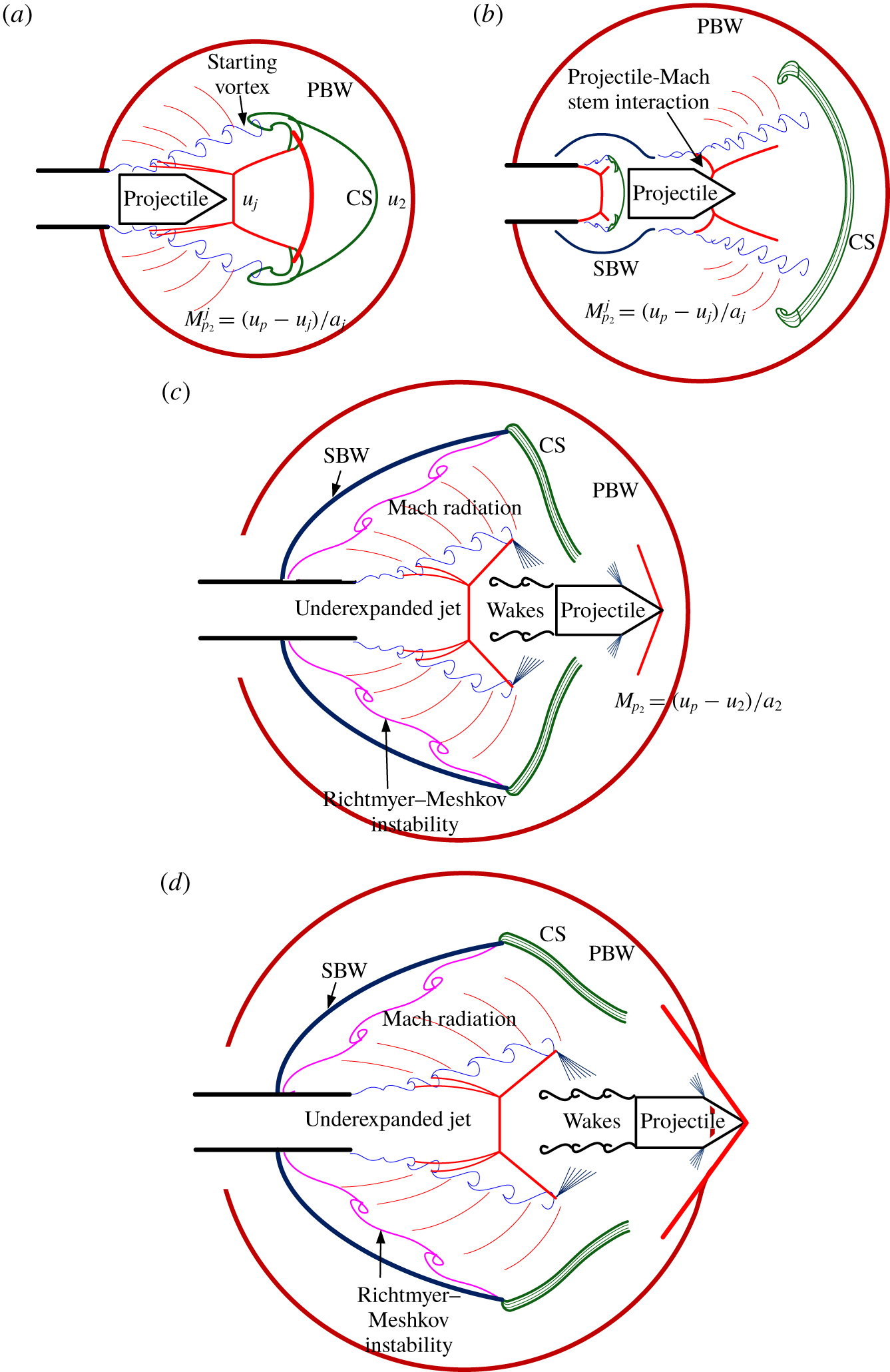
Schematic of the flow structures in the transitional ballistic regime. (a) Shock wave diffraction in an open-ended shock tube. (b) Projectile-unsteady jet interaction. (c) Shock generation due to a change in the relative Mach number ( $M_{p_{2}}$) of the projectile. (d) Projectile overtaking phenomenon.

When the projectile starts moving inside the launch tube at very high acceleration, it compresses the air ahead of it. These compression waves coalesce to form a strong moving normal shock downstream of the launch tube. The normal shock gets diffracted at the exit of the launch tube as a near-spherical blast wave, which is termed as the primary blast wave (PBW). The primary blast wave is followed by a contact discontinuity (contact surface – CS), with associated vortex rings (formed due to the rolling up of the boundary layer at the exit of the launch tube), which distinguishes the unsteady jet from the post-PBW flow. The unsteady jet is created by the launch tube gas expanding to the post-primary blast wave flow. The contact discontinuity refers to an interface between atmospheric air which has already been perturbed by the primary blast wave and the air jet exiting from the launch tube in front of the projectile. The pressure across the contact surface remains the same, in general, while there are discontinuities in velocity, density, temperature and entropy. The contact surface is diffused to the surrounding flow due to a momentum difference in the flow ahead and behind it as it propagates. The above scenario is a classical shock wave diffraction problem in an open-ended shock tube (Skews Reference Skews1967; Sun & Takayama Reference Sun and Takayama1997). Many researchers have studied the shock diffraction process in an open-ended shock tube and observed a characteristic feature that a second shock structure is present in the unsteady jet in order to ensure the pressure matching condition if the primary blast wave Mach number is greater than 1.3 for air (Sun & Takayama Reference Sun and Takayama1997). A schematic of the shock diffraction process is shown in figure 1(a).
The accelerated projectile is discharged to the unsteady jet. The unsteady jet from the launch tube can be subsonic or supersonic depending on the unsteady jet relative Mach number which is defined as  $(u_{j}-u_{2})/a_{2}$, where
 $u_{j}$ is the jet velocity,
 $u_{2}$ is the velocity of the bulk flow induced by the primary blast wave and
 $a_{2}$ is the speed of sound in the bulk flow. Though the unsteady jet velocity is unknown, subsonic and supersonic jets can be identified from the wave structures. When the projectile is discharged into the supersonic unsteady jet, it interacts with the wave structures as shown in figure 1(b), and its relative Mach number changes accordingly within the unsteady jet itself.
When the projectile passes through the unsteady jet, the relative Mach number of the projectile with respect to the unsteady jet decides the flow structures around it. Depending on the relative Mach number of the projectile, there can be an attached or detached or no shock on the projectile. Initially, when the projectile gets discharged from the tube, it passes through the unsteady jet and, therefore, the relative velocity is with respect to the jet velocity. Here, the relative projectile Mach number is defined as  $M_{p_{2}}^{j}$, which is equal to
 $(u_{p}-u_{j})/a_{j}$, where
 $u_{p}$ is the projectile velocity and
 $a_{j}$ is the sound speed in the jet flow. As the projectile moves further, it passes through the contact surface and the relative projectile Mach number now changes to
 $M_{p_{2}}$, defined as
 $(u_{p}-u_{2})/a_{2}$, i.e. with respect to the post-shock flow (figure 1c). In the case of a supersonic jet ahead of the projectile when it is discharged from the launch tube, it so happens that the relative Mach number of the projectile may not be supersonic to generate a shock wave in front of the projectile. However, when the projectile crosses the CS, its relative Mach number may become supersonic leading to the formation of a bow/oblique shock (figure 1c).
While this may be happening at the front of the projectile, the high pressure gas behind the projectile is discharged immediately after the projectile discharges from the launch tube. This generates a secondary blast wave (SBW) followed by a contact discontinuity, which separates the gas in the barrel and the air processed by the secondary blast wave, followed by an underexpanded jet (Jiang et al. Reference Jiang, Takayama and Skews1998). If the projectile is moving with subsonic speed with respect to the laboratory frame of reference, it is observed that the secondary blast wave overtakes the projectile within a short range where the projectile is still passing through the unsteady jet. The projectile overtakes the secondary blast wave at a later instant as the secondary blast wave keeps on attenuating and the projectile velocity is almost the same due to the high inertia that the projectile possesses. This kind of behaviour is reported in the case of supersonic projectiles with high Mach numbers (Rajesh et al. Reference Rajesh, Kim and Setoguchi2008). As the secondary blast wave expands further, it radially develops and passes over the interface between the unsteady jet and the post-primary blast flow (the diffusing contact surface) and results in the formation of the Richtmyer–Meshkov instability (RMI) (figure 1c,d). Richtmyer–Meshkov instability occurs whenever there is a misalignment between the density gradient and the impulsive pressure gradient vectors. A typical example would be a shock wave propagation from a light fluid to a dense fluid ( $\unicode[STIX]{x1D735}\unicode[STIX]{x1D70C}\boldsymbol{\cdot }\unicode[STIX]{x1D735}p<0$) or from a heavy fluid to a light fluid (
 $\unicode[STIX]{x1D735}\unicode[STIX]{x1D70C}\boldsymbol{\cdot }\unicode[STIX]{x1D735}p>0$) (Zhou Reference Zhou2017). When a pressure gradient is applied across the density gradient (the flow interface) by the propagation of the shock wave, it leads to the generation of the vortical structures on the interface leading to roll-up. In the present scenario, both the contact surface and the secondary blast wave are curved, and there is a possibility of the generation of the vortical structures leading to RMI (Jiang Reference Jiang2003). By this time, the projectile might overtake the secondary shock in the unsteady jet and contact discontinuity behind the primary blast wave. Now the projectile starts overtaking the primary blast wave (figure 1d).
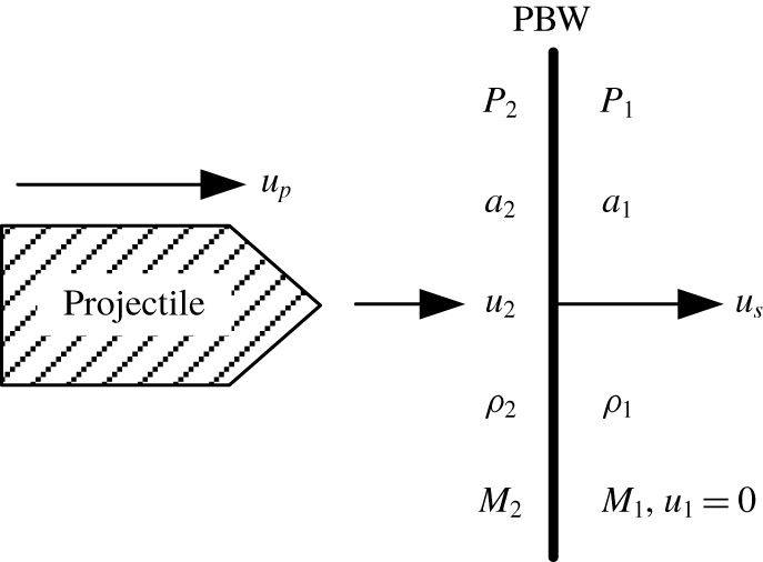
One-dimensional approximation of the primary blast wave as a moving normal shock wave followed by the projectile.

The projectile overtaking phenomenon refers to the unsteady scenario that the primary blast wave Mach number ( $M_{s}=u_{s}/a_{1}$, where
 $u_{s}$ is the velocity of the PBW and
 $a_{1}$ is the speed of sound in the undisturbed atmospheric air) is less than the projectile Mach number (
 $M_{p_{1}}=u_{p}/a_{1}$) (figure 2) and, therefore, the projectile overtakes the primary blast wave after all the projectile-flow interactions inside the primary blast wave as described above. This phenomenon is perceived as a shock–shock interaction by Watanabe et al. (Reference Watanabe, Fujii and Higashino1995) where the shock in front of the projectile along with it interacts with the moving primary blast wave in an unsteady manner. They numerically simulated the interaction of the projectile with the primary blast wave and categorized the overtaking phenomenon as subsonic and supersonic overtaking based on the relative projectile Mach number (
 $M_{p_{2}}$). If the relative Mach number of an overtaking projectile is greater than 1, it is termed as supersonic overtaking and if
 $M_{p_{2}}$ is less than 1, it is a case of subsonic overtaking (Watanabe et al. Reference Watanabe, Fujii and Higashino1995). Each type of overtaking may lead to various kinds of aerodynamic loading on the projectile. Similar studies have been carried out by Ahmadikia & Shirani (Reference Ahmadikia and Shirani2005) and confirmed the possibilities of drastic reduction in projectile drag after the projectile overtakes the primary blast wave due to favourable pressure conditions. Rajesh et al. (Reference Rajesh, Kim and Setoguchi2008) simulated the projectile overtaking phenomenon taking the blast wave attenuation into consideration, and came to a conclusion that a low primary blast wave Mach number at the time of overtaking will not affect the aerodynamic characteristics of the projectile in a noticeable manner. However, it is reported that the overtaking phenomenon has a profound impact if the overtaking happens in the close vicinity of the launch tube when the projectile and the primary blast wave Mach numbers are high enough.
It can be seen from the above discussion that the projectile aerodynamic characteristics in the near field of the muzzle exit of a launching device are quite complicated involving shock–shock interactions, projectile-unsteady jet interactions and projectile-shock interactions (unsteady shock diffraction). The transitional ballistic regime is also identified as one of the main sources of the projectile dispersion as it contains the above projectile interactions. Experimental studies are sparse and also of very low spatial and temporal resolutions from which useful projectile and flow data can be hardly deducted. The available computational studies lack proper validation and do not reveal realistic projectile-flow fields owing to the ambiguous conjectures.
Hence, the main objective of the present study is to experimentally understand the complicated flow features associated with a moving projectile in the transitional ballistic regime at high temporal and spatial resolutions for various flow field and projectile parameters. The study is focused on capturing the flow fields with high accuracy and resolving the projectile-flow field interactions such as the overtaking phenomenon and the unsteady projectile-shock interactions.
Experiments are carried out with various projectile configurations and blast wave Mach numbers and the flow fields are captured using time-resolved schlieren and shadowgraph techniques. The trajectories of the projectile and the blast wave have been obtained from the experimental pictures using image processing through edge detection algorithms. The results are thought to be helpful in understanding the source of the transient loads on the projectile which give rise to dispersion due to the blast disturbances. The data obtained will be useful to quantify the projectile aerodynamic characteristics when it passes through the transitional ballistic regimes, which are helpful for the projectile designers to estimate and reduce the dispersion of the projectile in various applications. The present work would also serve as an excellent database for validating unsteady CFD codes which deal with complicated flow processes such as shock–shock interaction, shock-moving body interactions and various flow instabilities in non-stationary flow fields.
2 Methodology
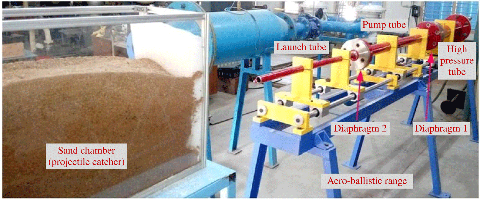
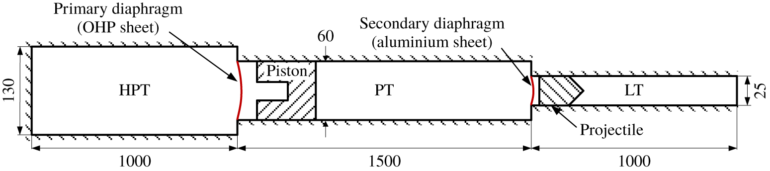
The flow characteristics associated with a moving projectile in the transitional ballistic regime is experimentally studied using an aero-ballistic range (figure 3) which is used to accelerate the projectile. The range consists of three sections, namely, the high pressure tube (HPT), the pump tube (PT) and the launch tube (LT) (figure 4). The required pressure to accelerate the projectile is generated in two stages, where the first stage is the shock compression behind the moving piston (a 1.57 kg stainless steel block) by the air in the high pressure tube and the second stage refers to the isentropic compression of the pump tube air by the moving piston.
Experimental set-up – aero-ballistic range.

Schematic representation of aero-ballistic range (all dimensions in mm).

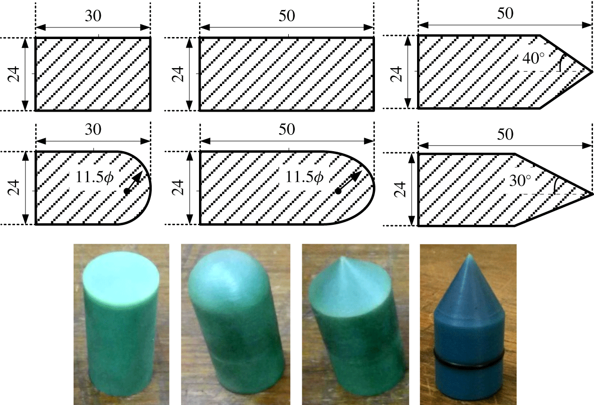
Projectiles having conical, cylindrical and hemispherical geometries of mass ranging from 11 to 16 g, made of metal cast nylon material are employed in the experiments. The dimensions of projectile configurations used in the experiments are shown in figure 5.
Projectile geometries (all dimensions in mm). Additional geometries are mentioned in table 1.

An air compressor of maximum 30 bar pressure capacity provides pressurized air to the high pressure tube. Upon sudden rupture of the primary diaphragm in the high pressure tube, the piston is accelerated to very high speeds and compresses the air in the pump tube to generate very high pressures (of the order of 250–300 bar) to rupture the secondary (aluminum) diaphragm (Rajesh et al. Reference Rajesh, Kim, Setoguchi and Raghunathan2007). The rupture of the secondary diaphragm initiates flow into the launch tube where the projectile is placed, and generates high pressure at the base of the projectile and accelerates it to high velocities inside the launch tube.
The emanating flow field at the end of the launch tube is captured using a time-resolved schlieren/shadowgraph optical flow visualization technique. A conventional Z-type arrangement with a halogen light source, two parabolic concave mirrors of 300 mm diameter and 2000 mm focal length, a vertical knife edge, a convex lens of 150 mm diameter and 480 mm focal length and an ultra-high-speed camera are used to carry out the experiments. Time-resolved images are captured using the Phantom v2512/IX-726 camera which is capable of recording images at  $25\,000/26\,000$ frames per second at full resolution of 1 mega pixels and a maximum of 1 million frames per second at reduced resolutions. The exposure times of both the Phantom v2512 and the IX-726 cameras are 1
 $\unicode[STIX]{x03BC}$s and 289 ns, respectively, which help to freeze the flow field and avoid the motion blur while quantifying the velocity data. Various frame speeds at various resolutions have been used to capture the projectile motion depending on the experimental conditions. The projectile motion and the associated flow structure are analyzed through processing of the time-resolved schlieren/shadowgraph images. The trajectories of both the primary blast wave and the projectile are reconstructed using image processing algorithms.
3 Results and discussion
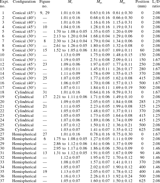
Experiments are conducted on projectiles of various configurations with various initial conditions (table 1). The configurations of the projectiles with half-cone angle (column 2) and length to diameter ratio (column 8) are listed in table 1. The corresponding figure numbers are indicated in column 3. Columns 4, 5 and 6 represent the Mach numbers of the PBW and the projectile along with the relative Mach number, respectively. Initially, the flow field is captured in the immediate vicinity of the launch tube and later the view field is shifted away from the exit of the launch tube in order to capture additional flow interactions. The distance of the view field away from the launch tube exit, corresponding to each experiment is indicated in column 7. Within this small visualization window, the projectile velocity remains almost constant due to the high amount of inertia it possesses when it comes out of the launch tube. The secondary diaphragm pressure ratio is controlled in the experiments using various diaphragms such as plastic and aluminum sheets of different thicknesses (0.9–1.5 mm) to obtain different projectile Mach numbers ranging from subsonic to supersonic.
Summary of the experiments conducted.

3.1 Flow features of supersonic projectile discharge
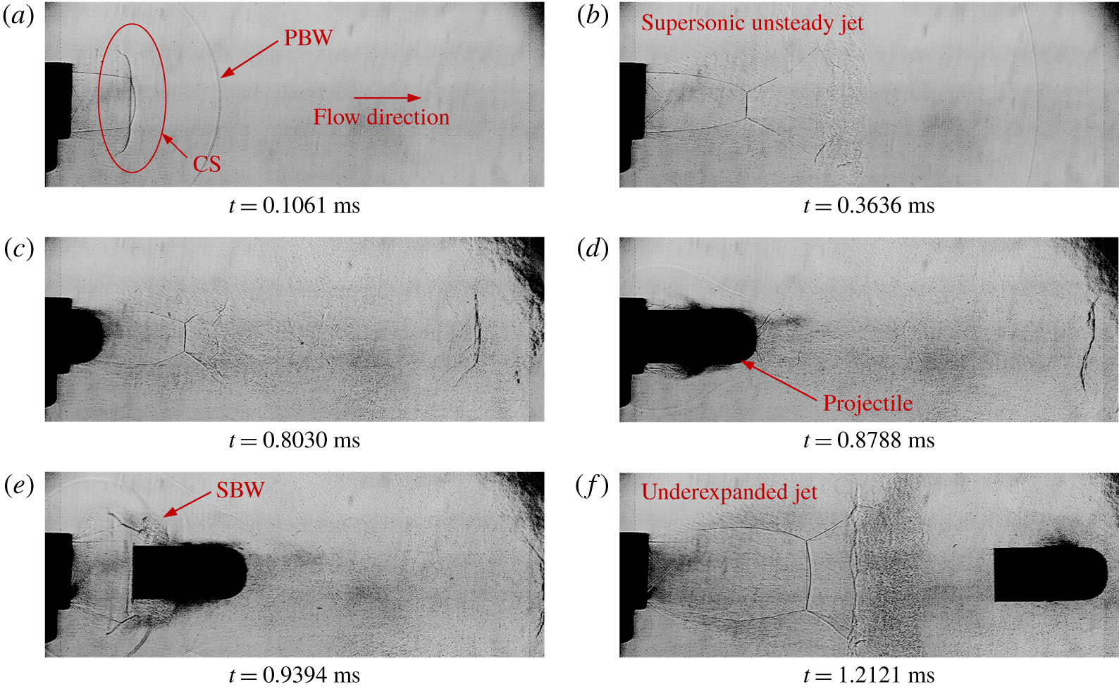
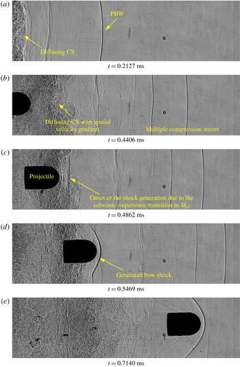
Shadowgraph images of a hemispherical projectile moving at a supersonic Mach number of  $1.27\pm 0.05$. (Images are captured with a resolution of
 $780\times 296$ at 66 000 fps, calibrated to
 $0.2706\pm 0.0034~\text{mm}~\text{pixels}^{-1}$, test-28 in table 1.)

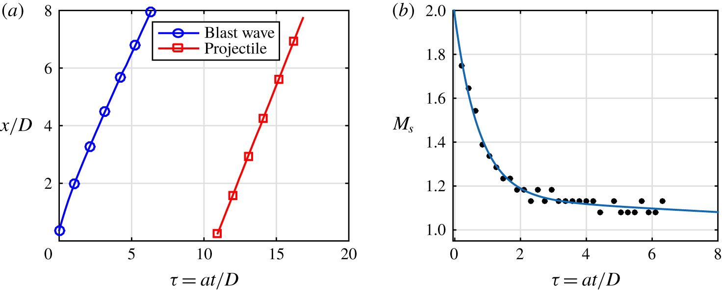
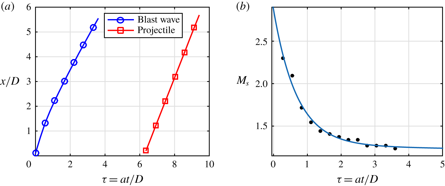
(a) Trajectories of the primary blast wave and the projectile. (b) Attenuation of the primary blast wave (corresponding to figure 6).

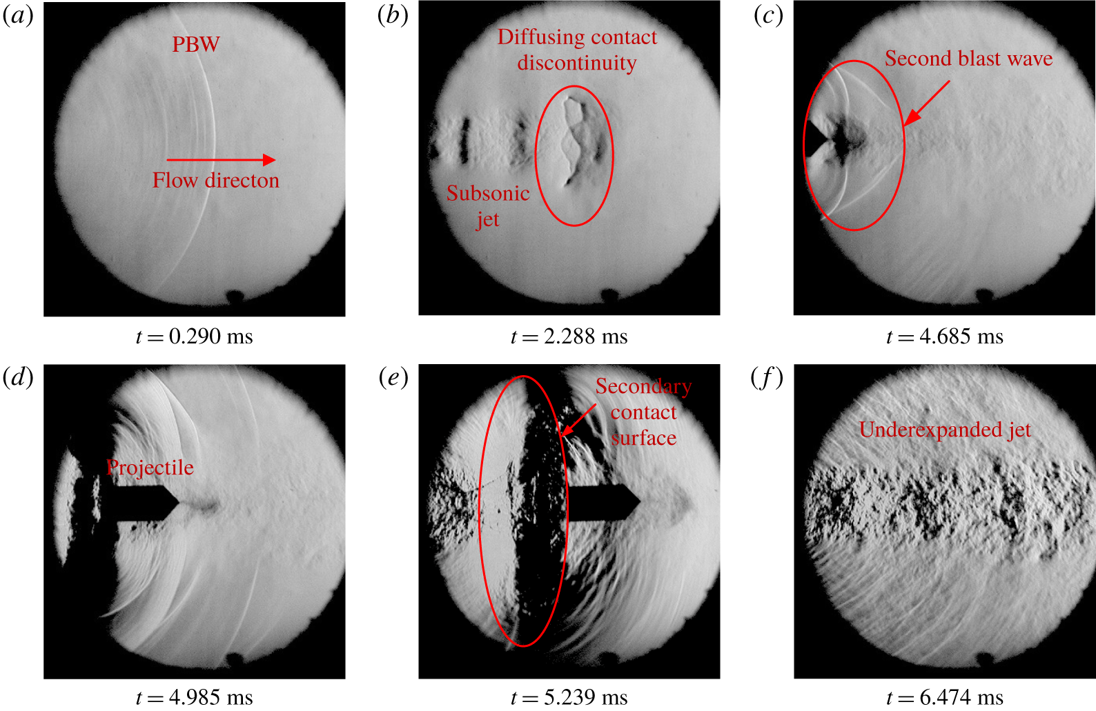
The time-resolved shadowgraph images of a hemispherical projectile moving with supersonic velocity ( $M_{p_{1}}>1$) is shown in figure 6 (test-28 in table 1). The frame on which the primary blast wave appears in the view field for the first time is considered as time instant
 $t=0$. The moving normal shock generated by the accelerated projectile inside the launch tube diffracts as a curved primary blast wave, and is captured in figure 6(a). The primary blast wave is followed by the contact discontinuity (figure 6a). Though the presence of contact discontinuity can be identified in the shadowgraph images, the associated flow structures such as the vortex rings and the vortex induced shock pair (Zhang et al. Reference Zhang, Aubry, Chen, Wu and Sha2019) are hardly noticeable. The unsteady jet emanating due to the discharge of launch tube air is underexpanded with visible shock cells (figure 6b). The projectile is launched to this supersonic jet (figure 6c). The view field is close to the launch tube exit and the projectile is passing through the supersonic unsteady jet within the visible region. In this regime, the moving projectile interacts with the Mach stem, which results in an unsteady shock diffraction phenomenon. In the well-known shock diffraction phenomena over bodies of various configurations (Skews Reference Skews2005), the moving normal shock passes over stationary bodies. The present scenario is different where the moving body passes through a normal shock which is stationary. In figure 6(d) the stationary Mach stem in the jet is seen to be diffracting over the moving projectile. The situation is described in more detail in the following subsection. Behind the projectile, the highly compressed pump tube gas is discharged with an associated secondary blast wave and a secondary contact discontinuity (figure 6e,f). The projectile may experience a significant reduction in the acceleration at this point as the flow has suddenly expanded behind the projectile. The interaction of the secondary blast wave with the projectile can be seen in figure 6(e). At a later instant, the projectile completely moves ahead of the continuously attenuating secondary blast wave. The secondary contact discontinuity is followed by the underexpanded jet (figure 6f).
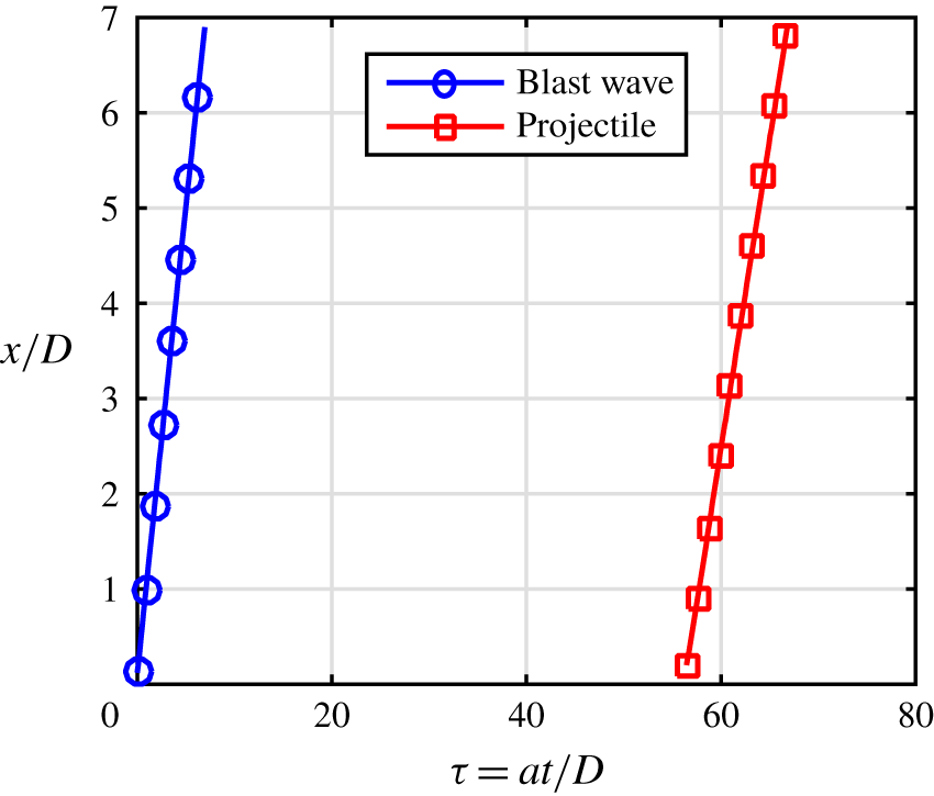
The corresponding trajectories of the blast wave and the projectile are constructed by processing the captured images and are shown in figure 7(a), where  $x$ is the distance from the exit of the launch tube,
 $D$ is the inner diameter of the launch tube and
 $a$ is the speed of sound in the undisturbed air. The projectile is found to be moving with constant velocity as the projectile trajectory is a straight line. The average velocity of the hemispherical projectile (
 $u_{p}$) in this case is
 $440.80\pm 18.72~\text{m}~\text{s}^{-1}$ (
 $M_{p_{1}}=1.27\pm 0.05$). The preceding primary blast wave is attenuating in nature as the trajectory has a higher slope immediately outside the launch tube and the slope reduces towards the end of the visualization window. As the primary blast Mach number is reducing fast due to the blast attenuation, the instantaneous velocities of the primary blast wave are calculated. This is estimated from the successive images by measuring the distance travelled by the blast between consecutive frames. The speed of sound in the stagnant atmosphere in the laboratory is taken as
 $347.27~\text{m}~\text{s}^{-1}$ in all the calculations. The primary blast wave Mach number (
 $M_{s}$) variation with respect to time is plotted in figure 7(b). A curve is fitted along with the experimentally obtained values in order to understand the general trend followed by the attenuating blast wave. Furthermore, a dimensional analysis is carried out for the blast wave decay (appendix A) in order to understand the effect of various non-dimensional parameters.
It is observed that the attenuation is larger and faster in the immediate vicinity of the launch tube and asymptotically reaches a sonic Mach number after a short period. The projectile Mach number ( $M_{p_{1}}$) is calculated from the average velocity, as there is no significant change in the instantaneous velocities. On the other hand, the projectile relative Mach number is continuously varying as it is a function of
 $M_{p_{1}}$,
 $M_{s}$ and
 $\unicode[STIX]{x1D6FE}$, and the primary blast wave is attenuating. In the present experiments, it is noticed that, by the time the projectile reaches the visualization window, the blast wave has either attenuated to a constant Mach number or already moved further away from the visualization window. This can be observed from the trajectory plot in figure 7(a). During the travel of the projectile through the visualization window, the variation in
 $M_{s}$ becomes insignificant owing to which, the changes in the relative Mach number of the projectile (
 $M_{p_{2}}$) can also be neglected. The value of
 $M_{p_{2}}$ is hence calculated using the final value (the attenuated value) of the blast Mach number. In the above-mentioned experiment, the blast Mach number varies from
 $1.75\pm 0.05$ to
 $1.08\pm 0.05$ (
 $u_{s}=609.10\pm 18.53$ to
 $375.00\pm 18.53~\text{m}~\text{s}^{-1}$) within the visible area. The value of
 $M_{p_{2}}$ is
 $1.11\pm 0.09$, which is calculated using the average projectile Mach number (
 $M_{p_{1}}=1.27\pm 0.05$) and the attenuated blast Mach number (
 $M_{s}=1.08\pm 0.05$).
Even though the blast Mach number is greater than the projectile Mach number at the launch tube exit, the blast Mach number reduces to a value less than that of the projectile Mach number ( $M_{p_{1}}$), which implies that the projectile will eventually overtake the blast. The overtaking can be subsonic (
 $M_{p_{1}}>1$ and
 $M_{p_{2}}<1$) or supersonic (
 $M_{p_{1}}>1$ and
 $M_{p_{2}}>1$) depending on the value of
 $M_{p_{2}}$. In this particular case,
 $M_{p_{2}}$ is in the transonic regime, and cannot be exactly distinguished as subsonic or supersonic as these are within the error band in the measured Mach number. The flow features associated with the subsonic overtaking are almost similar to that of supersonic overtaking, except for the presence of a shock structure in front of the projectile as it passes through the post-primary blast flow in the case of supersonic overtaking. However, as the relatively subsonic projectile (
 $M_{p_{1}}>1$ and
 $M_{p_{2}}<1$) overtakes the primary blast wave, it enters the free flight regime where the relative projectile Mach number changes to supersonic (as it is with respect to the ambient conditions), leading to the appearance of a shock wave. The subsonic overtaking rarely happens as the duration for which the relative projectile Mach number remains to be less than one is small due to the rapid attenuation of the primary blast wave (Rajesh et al. Reference Rajesh, Kim and Setoguchi2008). As a result of this, the experiments failed to capture the flow structures for subsonic overtaking as they resulted in either supersonic overtaking or impossible overtaking situations, even with multiple attempts with the extended visualization window.
In figure 6, where the view field is close to the launch exit, the projectile is moving inside the underexpanded unsteady jet. Hence, the relative projectile Mach number based on the jet velocity ( $M_{p_{2}}^{j}$) will not be equal to the value calculated using the post-shock conditions of the primary blast wave. Figures 1(a), 1(b) and 1(c) schematically show the change in the relative Mach number of the projectile during its travel from the launch tube exit to a location where it crosses the contact discontinuity. The absence of a preceding bow shock indicates that the relative Mach number of the projectile with respect to the unsteady jet (
 $M_{p_{2}}^{j}$) is clearly subsonic.
3.1.1 Unsteady shock diffraction and interaction with the secondary blast wave
Shadowgraph images of a conical projectile moving at a supersonic Mach number of  $1.79\pm 0.04$. (Images are captured with a resolution of
 $600\times 500$ and 50 193 fps, calibrated to
 $0.2375\pm 0.0016~\text{mm}~\text{pixels}^{-1}$, test-7 in table 1.)

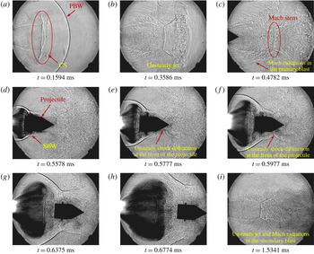
The flow features captured on a conical projectile are shown in figure 8 (test-7 in 1). It is observed that the flow features are quite similar to that of the hemispherical projectile shown in figure 6. The Mach radiation (Mach lines generated due to the interaction of the supersonic jet boundary with the surrounding flow) from the vortical structures in the shear layer as depicted schematically in figures 1(a), 1(b) and 1(c) are clearly visible (figure 8b,c,i). Apart from that, the unsteady shock diffraction is also seen clearly in figures 8(c–h) when the projectile passes through the Mach disk in the underexpanded jet behind the primary blast wave. The unsteady jet exits as a part of the primary blast wave as explained early. The unsteady jet extends up to the contact discontinuity behind the primary blast wave. The jet structure and the Mach stem height depend on the jet pressure ratio, which is defined as the ratio of the static pressure of the jet at the exit of the launch tube to the ambient pressure to which the jet exits. The ambient pressure is the post-shock pressure of the primary blast wave. The projectile is discharged to this unsteady underexpanded supersonic jet. As the projectile passes through the jet, it interacts initially with the expansion fan at the launch tube exit. There will be corresponding changes in the aerodynamic loads acting on the projectile as it passes through the expansion fan. The net aerodynamic load depends on the projectile geometry and the jet structure which is unsteady in nature. The projectile then encounters the Mach stem, which is a standing cylindrical shock within the axisymmetric jet (see figure 1c). This interaction is termed as the unsteady shock diffraction process as the projectile is a moving body which passes through the standing normal shock, which is contrary to the classical shock diffraction phenomenon where the moving shock passes over the stationary body. Being an axisymmetric body, the projectile interacts with the Mach stem symmetrically in an ideal situation. It can be seen that the interaction does not seem to generate similar flow features as that of the classical shock diffraction problem which is approximated through a coordinate transformation as a pseudo-steady/unsteady reflection of a planar shock moving over bodies (Ben-Dor Reference Ben-Dor2007). There are no patterns observed for a pseudo-steady/unsteady regular shock reflection. The shock is found becoming curved when it passes over the conical surface of the projectile (figure 8f). Though this is one of the important features of an apparent Mach reflection in pseudo-steady/unsteady shock reflections, the Mach stem, which is, in general, normal to the reflecting surface, and the reflected shock which are present in the pseudo-steady/unsteady Mach reflection are hardly identifiable in the visualization pictures. This may be due either to the absence of a pseudo-steady/unsteady Mach reflection or the fact that the projectile tip is moving into a perturbed region where the contact discontinuity is continuously diffusing, while the shock is getting diffracted over the projectile.
While this is happening at the front side of the projectile, something similar to the classical (stationary) shock diffraction happens at the rear side of the projectile. Immediately after the projectile discharge from the launch tube, the pump tube gas exits to the atmosphere with an associated secondary blast wave, contact surface and an underexpanded jet. During the initial stages of the projectile motion, the secondary blast is observed to be moving over the projectile (figure 8d). If the velocity of the secondary blast wave ( $u_{s_{2}}$) is higher than the projectile velocity (
 $u_{p}$) it will pass over the projectile. It can be seen from figures 8(d), 8(e) and 8(f) that the secondary blast and projectile have comparable velocities. However, the secondary blast might have been faster in the earlier frames (not shown) when it was developed behind the projectile initially. Due to this, it might have passed over the projectile and is now travelling along with the projectile with a comparable velocity. Considering the relative velocity of the secondary blast with respect to the projectile (
 $u_{s_{2}}-u_{p}$) in the earlier frames, this passing over is a case of a curved shock wave getting diffracted over a stationary blunt body (the rear side of the projectile appears to be a blunt body for the curved portion of the secondary blast) in a classical (stationary) shock diffraction fashion. Hence, during this period, the projectile may experience highly unsteady aerodynamic loads as the net axial force on the projectile is the result of two complicated phenomena; the one at the projectile front is an unsteady shock diffraction problem, and the other at the rear side is a classical (stationary) shock diffraction problem. The relative velocity,
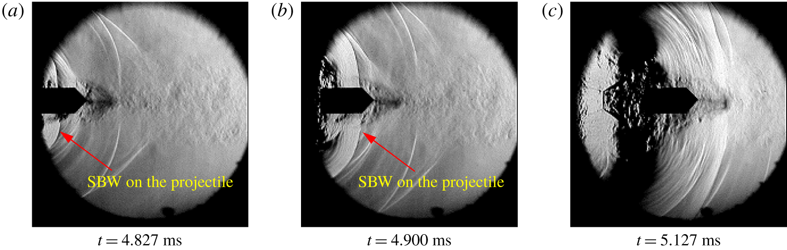
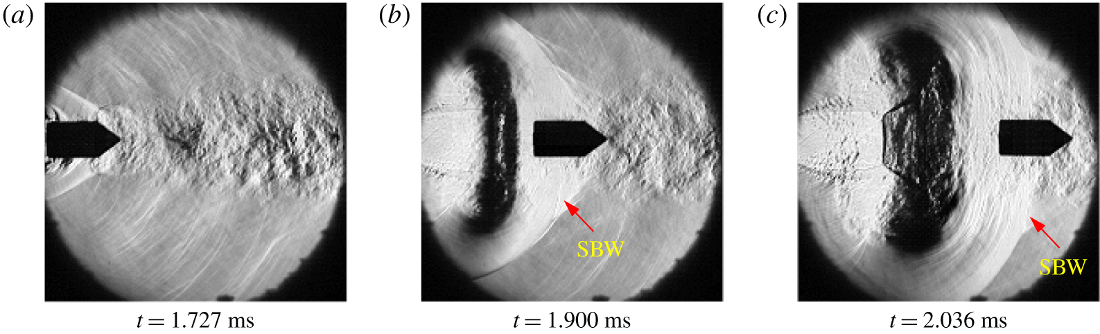
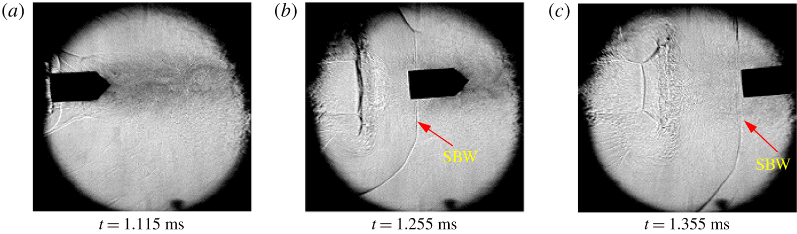
 $u_{s_{2}}-u_{p}$, may vary from positive to zero and finally to negative as the secondary blast develops, depending on launch conditions. For subsonic projectiles, this relative velocity mostly remains as positive at least in the transitional ballistic regimes as seen in some of the experiments (shown in figure 9), but for transonic or supersonic projectiles, the relative velocity is either positive, zero or negative (figures 10 and 11) for most of the projectile travel in the transitional ballistic regime.
Schlieren images of a subsonic projectile interacting with a secondary blast wave (SBW) ( $M_{p_{1}}=0.63\pm 0.16$, test-1 in table 1).

Schlieren images showing a secondary blast wave standing on the projectile within the view field ( $M_{p_{1}}=1.28\pm 0.16$, test-4 in table 1).

Shadowgraph images of a projectile passing through the secondary blast wave ( $M_{p_{1}}=1.47\pm 0.45$).

(a) Trajectories of the primary blast wave and the projectile. (b) Attenuation of the primary blast wave (corresponding to figure 8).

Jiang et al. (Reference Jiang, Takayama and Skews1998) reported that the diffracted shock at the front of the projectile is found to be focusing when it reaches the rear end of the projectile. Such a shock focusing is not observed here, probably due to the interference of the forward-moving, diffracting secondary blast and the associated unsteady jet structures present at the rear end of the projectile, which again depends on the projectile Mach number ranges considered.
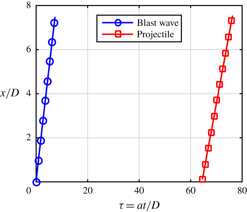
The trajectories of the blast wave and the projectile corresponding to figure 8 are shown in figure 12(a). In figure 12(b) we show the corresponding blast wave attenuation. The corresponding Mach numbers of the projectile and the blast wave are listed as test-7 in table 1. Here, the projectile Mach number is greater than the final Mach number of the blast wave ( $M_{p_{1}}>M_{s}$), which implies that the projectile will finally overtake the blast at a later instant, and the phenomenon can be classified as a supersonic overtaking as the relative projectile Mach number is supersonic (
 $M_{p_{2}}>1$). Even though the calculated
 $M_{p_{2}}$ is supersonic, similar to the experiment with the hemispherical projectile (figure 6), there is no preceding shock wave associated with the projectile. This means that the local relative Mach number is subsonic in figure 8. This is because the projectile in these pictures is moving within the unsteady supersonic jet (the relative projectile Mach number here is
 $M_{p_{2}}^{j}$) inside the view field. The possibility of overtaking phenomenon is further indicated by the converging nature of the
 $x$–
 $t$ diagrams (figures 7a and 12a).
3.1.2 Shock generation due to a change in the relative Mach number
Shadowgraph images of a hemispherical projectile moving at a supersonic Mach number of  $1.91\pm 0.05$ (images are captured with a resolution of
 $950\times 252$ and 65 822 fps, calibrated to
 $0.2558\pm 0.0029~\text{mm}~\text{pixels}^{-1}$, test-31 in table 1), with the view field 90 mm away from the launch tube exit.

Trajectories of the primary blast wave and the projectile corresponding to figure 13.

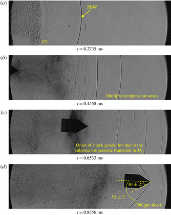
Shadowgraph images of a conical projectile moving at a supersonic Mach number of  $1.81\pm 0.07$ (images are captured with a resolution of
 $924\times 250$ and 65 822 fps, calibrated to
 $0.3197\pm 0.0044~\text{mm}~\text{pixels}^{-1}$, test-9 in table 1), with the view field 60 mm away from the launch tube exit.

Trajectories of the primary blast wave and the projectile corresponding to figure 15.

Shadowgraph images of a cylindrical projectile moving at a supersonic Mach number of  $1.71\pm 0.06$. (Images are captured with a resolution of
 $1000\times 250$ and 62 424 fps, calibrated to
 $0.3076\pm 0.0041~\text{mm}~\text{pixels}^{-1}$, test-19 in table 1.)

Trajectories of the primary blast wave and the projectile corresponding to figure 17.

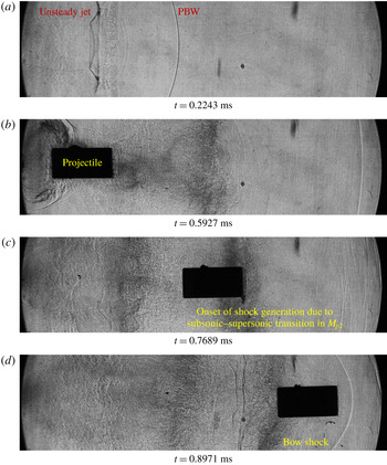
Further experiments are conducted in order to observe the absence of a preceding shock wave in front of the supersonic projectile when it is moving in the unsteady jet, and to confirm the presence of the shock wave at a later stage. The view field is slightly moved away from the launch tube exit in order to capture the interaction of the projectile and the contact surface in the primary blast wave. In figure 13 we show the hemispherical projectile passing through the visualization window which is 90 mm away from the launch tube exit. Along with the primary blast wave, there are multiple compression waves visible in front of the launch tube (figure 13b–d). This may be due to the non-uniform acceleration of the projectile inside the launch tube which is strong enough to produce multiple shock waves inside the tube itself. Multiple reflections of the compression waves generated by the rupture of the secondary diaphragm on the projectile base and piston front end might develop fluctuating projectile base pressures leading to non-uniform projectile acceleration. This effect may not be prominent in the case of subsonic projectiles since the acceleration of the projectile inside the launch tube itself is less and the compression caused by the instantaneous accelerations of the projectile may not be strong enough to generate multiple shock waves. The one-dimensional approximations, used to calculate the post-shock velocity in the primary blast and the relative Mach number of the projectile ( $M_{p_{2}}$) do not consider the presence of the multiple compression waves, instead it takes into account only the primary blast wave properties.
In figure 13(a) we show the primary blast wave and the associated flow structures preceding the launch of a hemispherical projectile. The contact surface is diffusing to the surrounding post-shock flow. The diffusion process involves turbulent mixing between the post-shock flow and the unsteady jet, which is a three-dimensional phenomenon. The schlieren/shadowgraph images indicate the flow field interactions happening in a plane and, therefore, will not be able to capture the non-axisymmetric nature of the contact surface diffusion. Gradients of density, velocity, temperature and entropy may hence be present in all the spatial directions. The projectile discharged to the unsteady jet is visible in figure 13(b), where the relative projectile Mach number seems to be subsonic as there is no visible shock structures in front of the projectile. This implies that the projectile is still in the unsteady jet, behind the contact surface as seen from the pictures, and the relative projectile Mach number is  $M_{p_{2}}^{j}$. In figure 13(c) we show the projectile motion through the diffused contact surface which has a transient spatial Mach number gradient owing to the mixing process. When the projectile is passing through this Mach number gradient, the relative velocity of the projectile is transitioning from
 $M_{p_{2}}^{j}$ to
 $M_{p_{2}}$, which is now decided primarily by the projectile velocity (
 $u_{p}$), the post-primary blast velocity (
 $u_{2}$) and the sound speed in the post-primary blast flow (
 $a_{2}$) (test-31 in table 1). The relative projectile Mach number in this case is now supersonic and a detached bow shock is seen in front of the projectile (figure 13d,e). The onset of the generation of this shock can be seen in figure 13(c) when the relative Mach number of the projectile is transitioning as it passes through the flow region where the spatial flow velocity gradient is present. Considering the aerodynamic characteristics of the projectile, this is an important event in the flow field as the aerodynamic load on the projectile suddenly increases upon the generation of the shock wave.
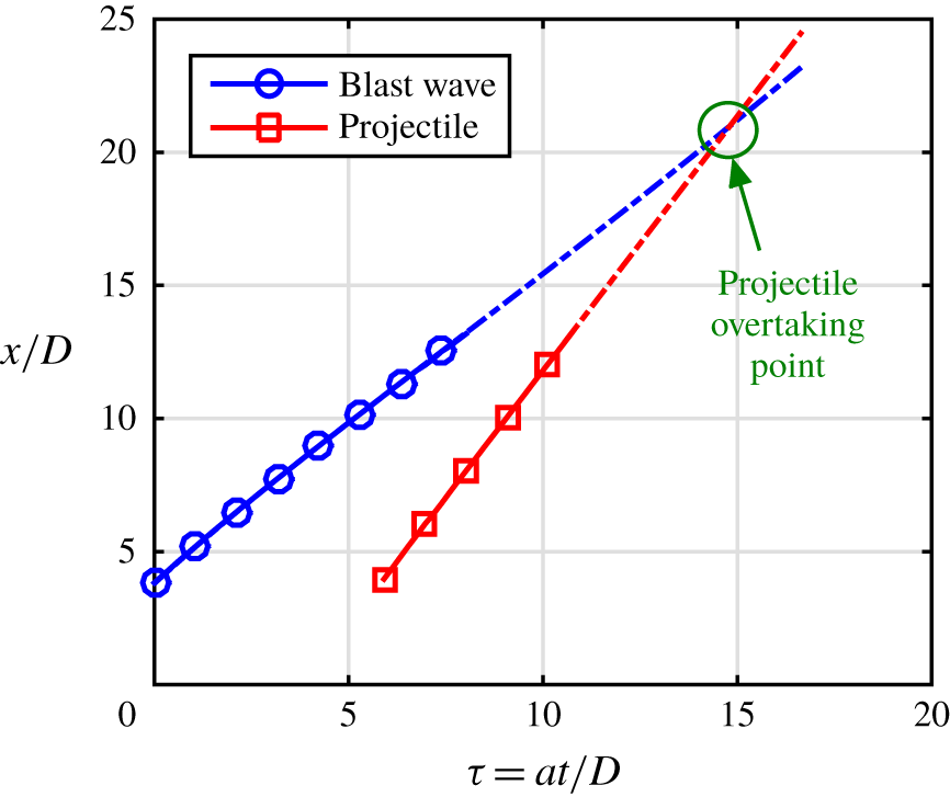
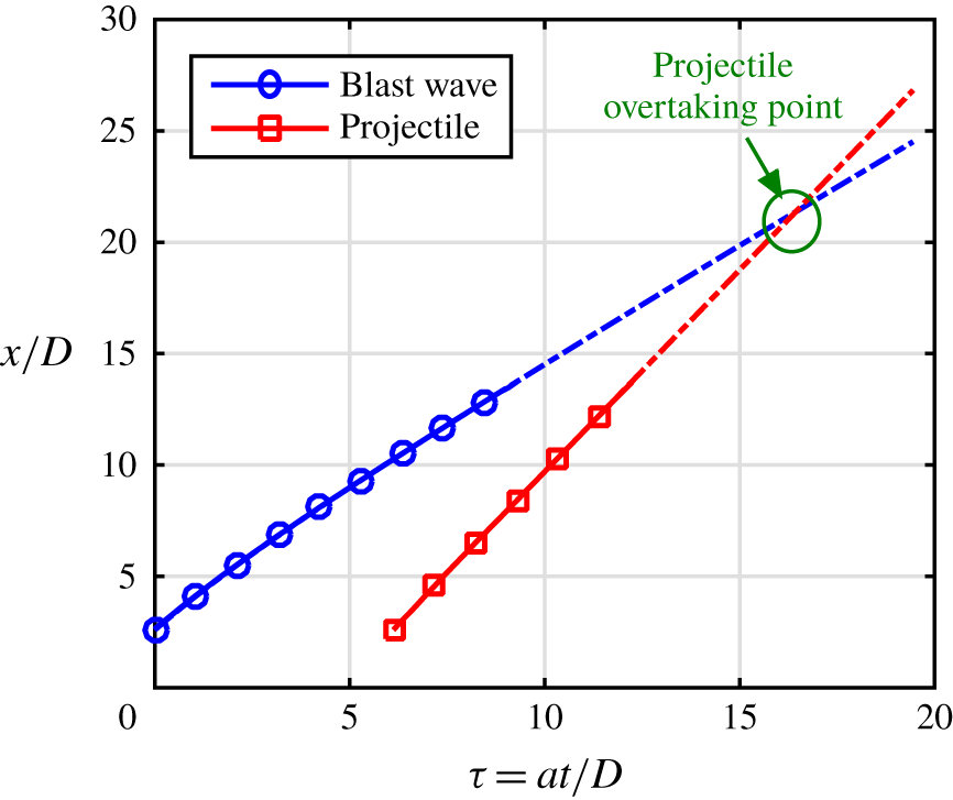
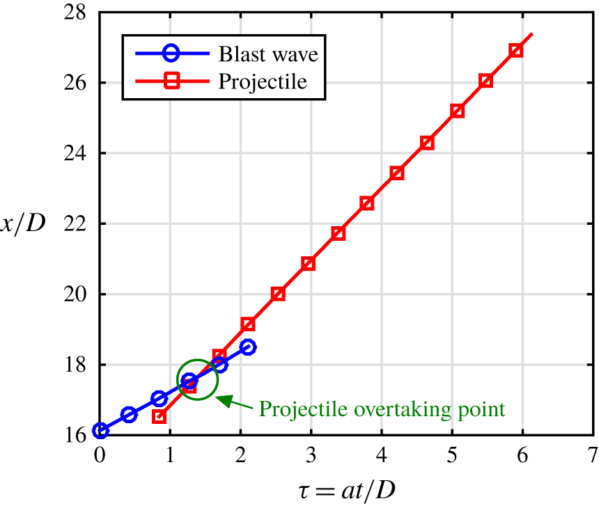
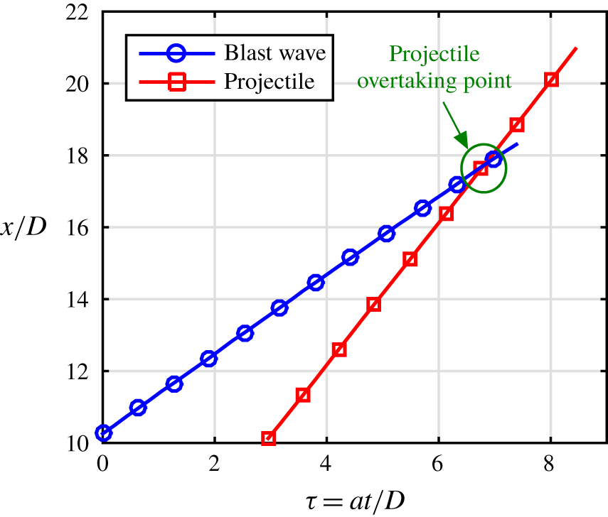
The trajectories of the blast wave and the projectile are plotted in figure 14. As the trajectories are converging in nature, the individual  $x$–
 $t$ diagrams are extrapolated to locate the position and time at which the overtaking phenomenon happens. The supersonic value of the relative Mach number implies that the experiment shown in figure 13 is a case of supersonic overtaking.
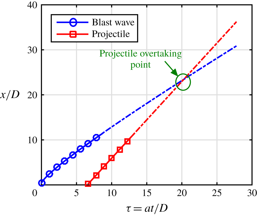
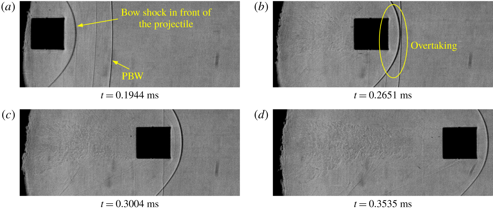
The flow features of a similar experiment conducted with a conical projectile are shown in figure 15 (test-9 in table 1). The  $x$–
 $t$ diagrams for both the blast wave and the projectile are now extrapolated and the overtaking point is calculated and marked in figure 16. This experiment also captured multiple compression/blast waves (figure 15b). The onset of the shock generation and the attached oblique shock are clearly visible (figure 15c,d). From the conical shock relations, for a projectile Mach number of 1.69 and the cone angle of
 $30^{\circ }$, the wave angle is
 $54.93^{\circ }$, which is in fairly good agreement with the measured wave angle of
 $53\pm 2^{\circ }$. The projectile is slightly pitched down in this case and the pitching angle is approximately
 $3^{\circ }$.
Another experiment conducted with the cylindrical projectile, where the view field is close to the launch tube exit, could also capture the generation of the bow shock (figure 17, test-19 in table 1). The extrapolated trajectories of the primary blast wave and the projectile are shown in figure 18. The flow features are similar to that of the hemispherical (figure 13) and conical (figure 15) projectiles. The only difference being the presence of the detached bow shock in front of the hemispherical and the cylindrical projectiles and an attached conical shock for the conical projectile, which purely depends on the geometry and the relative Mach number. Here also, the projectile will be overtaking the primary blast wave at a later instant and is a case of supersonic overtaking as obvious from the value of the  $M_{p_{2}}$ (test-19 in table 1).
3.1.3 Projectile overtaking phenomenon
Shadowgraph images of a hemispherical projectile moving at a supersonic Mach number of  $2.05\pm 0.07$ (Images are captured with a pixel resolution of
 $950\times 252$ and 65 822 fps, calibrated to
 $0.3574\pm 0.0055~\text{mm}~\text{pixels}^{-1}$, test-35 in table 1), with the view field 400 mm away from the launch tube exit.

Trajectories of the primary blast wave and the projectile corresponding to figure 19.

Shadowgraph images of a cylindrical projectile moving at a supersonic Mach number of  $2.23\pm 0.05$ (Images are captured with a resolution of
 $1070\times 252$ and 56 583 fps, calibrated to
 $0.2663\pm 0.0031~\text{mm}~\text{pixels}^{-1}$, test-21 in table 1), with the view field 325 mm away from the launch tube exit.

Trajectories of the primary blast wave and the projectile corresponding to figure 21.

Shadowgraph images of a conical projectile moving at a supersonic Mach number of  $1.97\pm 0.07$ (Images are captured with a resolution of
 $936\times 252$ and 65 822 fps, calibrated to
 $0.3224\pm 0.0044~\text{mm}~\text{pixels}^{-1}$, test-12 in table 1), with the view field 250 mm away from the launch tube exit.

Trajectories of the primary blast wave and the projectile corresponding to figure 23.

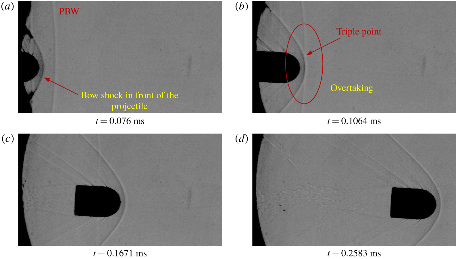
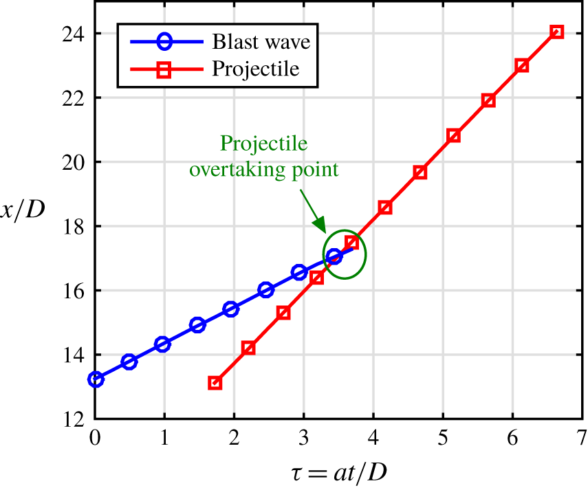
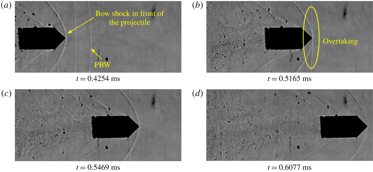
In order to visualize the overtaking phenomenon (the projectile overtaking the primary blast wave) experimentally, the view field is shifted further away from the launch tube exit. In figures 19, 21 and 23 we show the flow features when hemispherical, cylindrical and conical projectiles overtake the primary blast, respectively. The corresponding  $x$–
 $t$ diagrams are also shown in figures 20, 22 and24.
The projectiles are seen to be either slightly pitched up or down and, hence, created a leeward side and a windward side. The shadowgraph being two-dimensional, yaw could not be calculated properly. The merging of the two shock waves, i.e. the primary blast wave and the shock that is formed on the projectile, is clearly visible for all the three cases. It has to be noted that at the time of overtaking the blast wave has significantly attenuated and is almost similar to an acoustic wave. Hence, the overtaking may not have a significant effect on the aerodynamic characteristics of the projectile.
Projectile overtaking with the interaction of the oblique shock and the primary blast wave (shadowgraph images corresponding to test-15 in table 1).

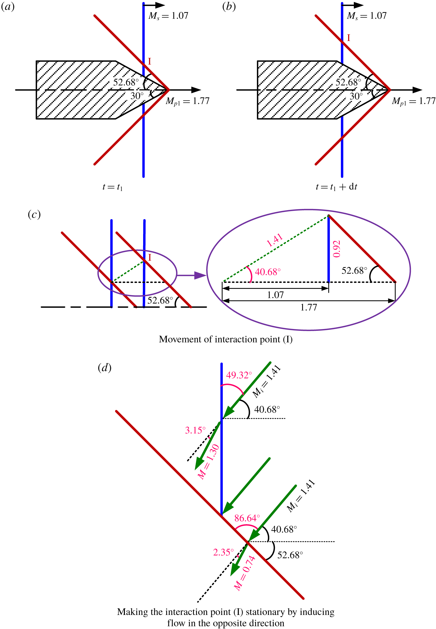
Schematic representation of the interaction point movement.

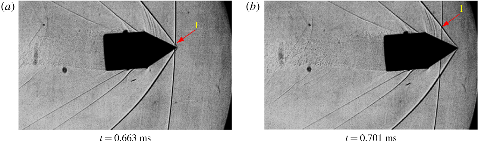
As seen from the above pictures, the overtaking phenomenon is a shock–shock interaction problem in which both the shocks are moving. Law, Felthun & Skews (Reference Law, Felthun and Skews2003) have analytically formulated and solved various shock-on-shock interaction problems and drawn useful conclusions on the types of reflections arising out of such interaction problems. In figure 25 we show the shadowgraph image of a conical projectile with a half-angle of  $30^{\circ }$. The Mach number of the projectile (
 $M_{p_{1}}$) and the blast wave (
 $M_{s}$) are
 $1.77\pm 0.05$ (
 $M_{p_{2}}=1.62\pm 0.08$) and
 $1.07\pm 0.05$, respectively (test-15 in table 1). In order to identify the type of shock–shock interaction, a pseudo-steady analysis (Law et al. Reference Law, Felthun and Skews2003; Law & Skews Reference Law and Skews2003) of the overtaking problem with respect to the Mach number (
 $M_{i}$) of the interaction point (I in figure 25) has been carried out as schematically shown in figure 26. The interaction point is moving over the oblique shock from the leading edge towards the trailing edge (figure 26a,b). The pseudo-steady analysis of the shock–shock interaction is performed by making the interaction point stationary and inducing a flow with Mach number of
 $M_{i}$ in the opposite direction of the propagation of the interaction point (figure 26d). The Mach number of the interaction point is calculated as shown in figure 26(c). In this case, the Mach number of the interaction point is 1.41 and is propagating at an angle of 40.68
 $^{\circ }$ with the horizontal. From the pseudo-steady analysis, the flow Mach number behind the oblique shock is subsonic as shown in figure 26(d) and, therefore, no regular or irregular reflections are possible at the interaction point. This is different from the images in figure 25, which shows a regular reflection like structure after the two shocks interact. One of the possible reasons for this is the three-dimensionality in the flow field which could not be captured by the two-dimensional flow visualization. In the real scenario, the blast wave will be near-spherical and the projectile may have yaw which makes the flow field three-dimensional. Now that the projectile might be moving out of the focal plane of the lens with an aperture of
 $f/2.0$ for which the depth of field is very small, the spatial density gradient generated by the near-spherical blast and the conical shock on the projectile might be misaligned with a two-dimensional light path in the shadowgraph system. This might give rise to additional shock structures in the flow field images even if the shock–shock interaction produced a subsonic flow downstream as depicted in figure 26(d). However, it can be concluded that the important flow features of the supersonic overtaking have been captured reasonably well in the shadowgraph pictures.
3.2 Flow features of subsonic projectile discharge
Schlieren images of a hemispherical projectile moving at a subsonic Mach number ( $M_{p_{1}}$) of
 $0.78\pm 0.16$ (
 $M_{s}=1.01\pm 0.16$,
 $M_{p_{2}}=0.75\pm 0.30$, images are captured with a resolution of
 $384\times 400$ and 110 000 fps, calibrated to
 $0.5111\pm 0.0116~\text{mm}~\text{pixels}^{-1}$, test-27 in table 1).

Trajectories of the primary blast wave and the projectile corresponding to figure 27.

Schlieren images of a conical projectile moving at a subsonic Mach number ( $M_{p_{1}}$) of
 $0.63\pm 0.16$ (
 $M_{s}=1.01\pm 0.16$,
 $M_{p_{2}}=0.61\pm 0.30$, images are captured with a resolution of
 $384\times 400$ and 110 000 fps, calibrated to
 $0.5111\pm 0.0116~\text{mm}~\text{pixels}^{-1}$, test-1 in table 1).

Trajectories of the primary blast wave and the projectile corresponding to figure 29.

Schlieren images of a cylindrical projectile moving at a subsonic Mach number ( $M_{p_{1}}$) of
 $0.64\pm 0.16$ (
 $M_{s}=1.01\pm 0.16$,
 $M_{p_{2}}=0.59\pm 0.30$, images are captured with a resolution of
 $384\times 400$ and 110 000 fps, calibrated to
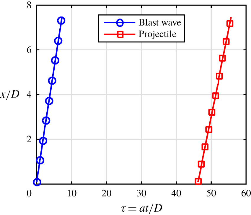
 $0.5111\pm 0.0116~\text{mm}~\text{pixels}^{-1}$, test-18 in table 1).

Trajectories of the primary blast wave and the projectile corresponding to figure 31.

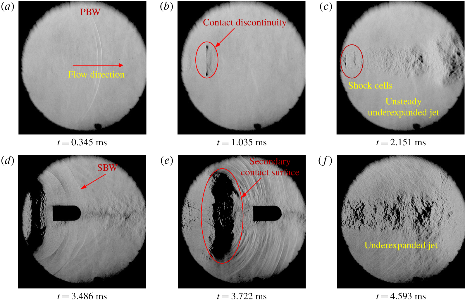
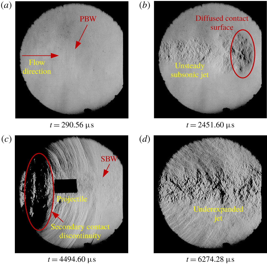
The above discussions were based on a supersonic projectile getting discharged from the launch tubes. The projectile discharging from the launch tube can be subsonic as well. In such flow fields, except the initial shock diffraction, the flow features are different from that of the supersonic projectile discharge. In figure 27 we show the flow structures associated with subsonic hemispherical projectiles. The primary blast wave is followed by the contact discontinuity which is marked in figure 27(b). The contact discontinuity is diffused to the surrounding flow as it moves forward. The launch tube gas ahead of the projectile is discharged as an unsteady jet following the contact discontinuity. This unsteady jet ahead of the projectile is underexpanded as seen in figure 27(c) with visible shock cells. The projectile is discharged to this unsteady jet. As the projectile moves out of the launch tube, the high pressure gas behind it, which was previously present in the pump tube, expands to the open atmosphere. This expansion develops the secondary blast wave followed by contact discontinuity and a highly underexpanded jet. The secondary blast wave is marked in figure 27(d). Since the projectile moves with a subsonic velocity, the secondary blast overtakes the projectile at a later instant, as can be seen in figure 27(e). This is an example of the stationary shock diffraction problem at the rear side of the projectile as explained early where the secondary blast velocity is larger than the projectile velocity. The contact surface separating the underexpanded jet from the preceding flow field is also clearly noticeable in this figure. A highly underexpanded jet with visible shock cells is seen in figure 27(f). In some cases, this unsteady jet also overtakes the projectile when the contact surface is moving over it. The jet pressure may produce significant aerodynamic loads on the projectile. The trajectories are traced through image processing for the primary blast wave and the projectile, and the corresponding  $x$–
 $t$ diagram is shown in figure 28.
Experiments conducted with the conical and cylindrical projectiles also reveal flow features similar to that of the above case and are shown in figures 29 and 31, respectively. One of the noticeable differences is that the unsteady jet in front of the projectile is found to be subsonic in the experiments due to a weakly accelerated projectile inside the launch tube (figures 29b and 31b). The absence of any type of shock waves can be observed on the projectile due to its relative subsonic flight. It can also be noted in figures 29(d) and 29(e) that the contact surface in the secondary blast is overtaking the projectile imparting the unsteady jet momentum on the projectile. The corresponding trajectories are plotted in figures 30 and 32 for the conical and cylindrical projectiles, respectively. In these experiments, the projectile Mach number is always less than that of the primary blast wave. It may also be noted from figures 28, 30 and 32 that the trajectories of the blast wave and the projectile are diverging in nature and, therefore, will never intersect, which implies that the projectile cannot overtake the blast wave as long as the blast wave attenuation is not significant within the investigation window and, therefore, lies in the impossible/no overtaking regime ( $M_{s}>M_{p_{1}}$).
The repeatability of the measured quantities could not be ensured as most of the experiments could not be repeated under the same conditions, as it depends on several factors, such as projectile dimensions, projectile weight, diaphragm thickness, depth of the diaphragm scoring and initial pressure. Therefore, a rigorous quantitative comparison of the experimental results has not been attempted in this work. It can be noticed from the experiments (table 1) that as the projectile Mach number ( $M_{p_{1}}$) increases, there is a corresponding increase in the shock Mach number (
 $M_{s}$) at the exit of the launch tube. The trend of increasing
 $M_{s}$ with increasing
 $M_{p_{1}}$ cannot be observed for various projectile configurations. For example, comparing test-8 and test-29 from table 1, where test-8 represents a conical projectile with a Mach number of 1.80 and test-29 represents a hemispherical projectile of 1.61 Mach number. It was expected that the primary blast wave corresponding to the conical projectile should be stronger than that of the hemispherical projectile. In contrary to the expectation, the experimental values for the primary blast wave initial Mach number were
 $M_{s}=2.61$ for the conical projectile and
 $M_{s}=2.86$ for the hemispherical projectile. Therefore, the trend of increasing
 $M_{s}$ with increasing
 $M_{p_{1}}$ holds for a particular configuration of the projectile, and cannot be compared for various shapes as the internal ballistics itself may vary according to the projectile configuration. Comparison of
 $M_{s}$ and
 $M_{p_{1}}$ values of a projectile in the impossible overtaking, subsonic overtaking and supersonic over taking regimes is illogical as the preceding flow features are extremely different for these cases, as described in the previous sections. Even though there is a quantitative discrepancy in obtaining a general or predictable trend between the experiments, it can be surely stated that the qualitative nature of the projectile-flow field interactions remains the same irrespective of the projectile configurations and launch initial conditions.
The aerodynamic characteristics of the projectile deviate significantly due to the above-mentioned projectile-flow field interactions as described using the acceleration-time history plot obtained from the numerical simulations of projectiles in the intermediate ballistic regime carried out by Rajesh et al. (Reference Rajesh, Kim and Setoguchi2008). In this work, the main emphasis has been given to the experimental identification of the flow structures in these crucial flow phenomena, which are (i) the unsteady shock diffraction on the projectile, (ii) the generation of shock waves when the relative Mach number changes from subsonic to supersonic values, and (iii) the projectile overtaking phenomenon.
A quantitative analysis of the drag characteristics of the projectile attempted was not successful. Instantaneous velocities and accelerations of the projectile have been calculated based on the  $x$–
 $t$ information obtained from the image processing. The error propagation upon successive differentiation of the
 $x$–
 $t$ relation of the projectiles to estimate the instantaneous accelerations and drag was large due to the non-negligible values of the error in the experiments. Moreover, in most of the experiments the change in instantaneous velocities of the projectile due to experimental error (appendix B) was larger than the actual change due to flow interactions. Hence, the obtained drag data were not reasonable.
4 Conclusions
The highly unsteady and complex flow phenomenon across a moving projectile in the transitional ballistic regime have been analyzed experimentally. The configuration effects of the projectile have also been taken into consideration. Even though the shape of the projectile possesses a great effect on the drag force acting on it, the fundamental flow interactions are irrespective of the configuration of the projectile. Time-resolved schlieren/shadowgraph images are used to generate the  $x$–
 $t$ diagrams for both the primary blast wave and the projectile. The blast disturbance effects that change the aerodynamic characteristics of the projectile have been qualitatively analyzed. The discharge of the compressed gas in the launch tube ahead of the projectile gives rise to a shock diffraction at the end of the launch tube with a primary blast wave, contact surface and unsteady supersonic jet and associated flow structures. As the projectile proceeds through the unsteady supersonic jet when it is out of the launch tube, it interacts with the shock cells in the underexpanded jet. The interaction of the moving projectile and the Mach stem is a kind of ‘unsteady shock diffraction’ phenomenon where the moving body interacts with a standing normal shock. The flow patterns are found to be different from that of the classical shock diffraction patterns over stationary bodies. The projectile is found subjected to differential loads owing to the unsteady shock diffraction at the projectile front side and the classical shock diffraction at the rear side where the secondary blast moves over the projectile. Another important phenomenon in the flow field is identified as the generation of the shock wave on the projectile when the projectile moves through the diffused primary contact discontinuity when the projectile relative Mach number becomes supersonic during this process. The projectile may now carry a shock wave when it overtakes the primary blast wave, referred to as a supersonic overtaking problem, leading to a moving shock on shock interaction (Law & Skews Reference Law and Skews2003; Law et al. Reference Law, Felthun and Skews2003). The present experiments reveal that the shock on shock interactions on projectiles within the Mach number range investigated are in the weak shock reflection domain where the downstream flow is subsonic. To the best of the authors knowledge, the present work may be the first of its kind that experimentally visualizes these kinds of phenomena happening in a highly transient flow environment.
A rigorous quantitative analysis of the aerodynamic characteristics of the projectile from image processing could not be carried out, as it requires optimization of the experimental setup such that the errors in the measurements should be less than the actual changes in the instantaneous velocities due to the flow interactions.
Declaration of interests
The authors report no conflict of interest.
Supplementary movies
Supplementary movies are available at https://doi.org/10.1017/jfm.2020.278.
Appendix A. Dimensional analysis
Dimensional analysis is performed on the blast wave decay using Buckingham’s pi theorem. The blast wave location from the launch tube exit ( $x$) can be written as a function of time (
 $t$), the speed of sound in the undisturbed air (
 $a$), the diameter of the launch tube (
 $D$) and the initial blast velocity at the launch exit (
 $u_{s_{0}}$). Therefore,
 $$\begin{eqnarray}\displaystyle f(x,t,a,D,u_{s_{0}})=0. & & \displaystyle\end{eqnarray}$$
The number of variables  $n=5$ (i.e.
 $x,t,a,D,u_{s_{0}}$) and the number of fundamental dimensions
 $=$
 $m=2$ (i.e. [L], [T]). By Buckingham’s theorem, the number of dimensionless groups
 $=$
 $n-m=5-2=3$.
Thus, the blast wave attenuation can be approximated with three dimensionless parameters such as non-dimensional distance ( $x/D$), the Mach number of the blast immediately at the launch tube exit (
 $M_{s_{0}}$) and the quantity (
 $at/x$). Therefore,
 $$\begin{eqnarray}\displaystyle \frac{x}{D}=f\left(M_{s_{0}},\frac{at}{x}\right). & & \displaystyle\end{eqnarray}$$
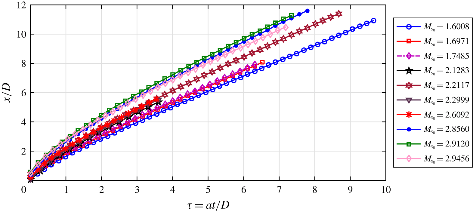
Because of the three  $\unicode[STIX]{x1D6F1}$ groups, it is hardly possible to derive a functional relationship among these parameters. In figure 33 we show the
 $x/D$ variation of the primary blast wave with respect to the non-dimensional quantity
 $at/x$ for various experiments with different initial blast wave Mach numbers (
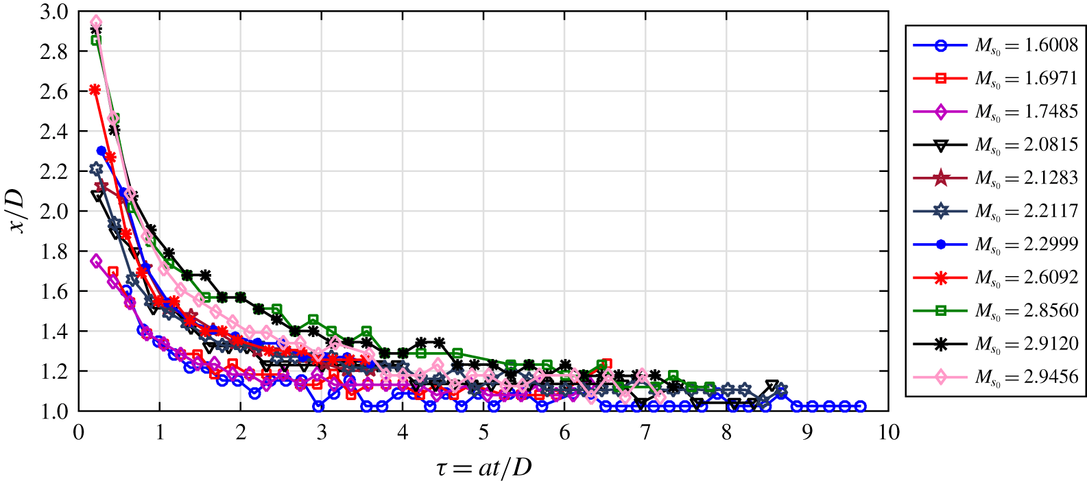
 $M_{s_{0}}$). From the dimensional analysis, it can be inferred that the Mach number (
 $M_{s}$) decay will be a function of
 $M_{s_{0}}$ and
 $at/D$. In figure 34 the Mach number variation is plotted. Hence, it can be concluded that within the range of experiments conducted, the blast wave attenuates towards a near acoustic wave before it starts interacting with the projectile. Even though the attenuation is strongly dependent on the starting Mach number (
 $M_{s_{0}}$), it finally attenuates to Mach 1, which is a well-known fact about blast waves. At the same time, the starting Mach number of the blast wave is a result of the internal ballistics, which is not in the scope of this study.
Blast wave trajectory.

Variation of the blast Mach number ( $M_{s}$) with respect to
 $at/D$.

Appendix B. Uncertainty analysis
B.1 Error in calibration
The experimental images are calibrated using a known dimension such as the base diameter of the projectile or the outer diameter of the launch tube. The error in the measurement of the actual length of the projectile is taken to be  $\pm 0.1~\text{mm}$ (the least count of the Vernier caliper used), i.e.
 $$\begin{eqnarray}\displaystyle & \displaystyle \text{d}l=\pm 0.1\quad \text{mm}, & \displaystyle\end{eqnarray}$$
 $$\begin{eqnarray}\displaystyle & \displaystyle \text{therefore, measured length}=l\pm \text{d}l\quad \text{mm}. & \displaystyle\end{eqnarray}$$
The corresponding number of pixels ( $pxl$) are counted from the edge detected image with an uncertainty of
 $\pm 1$ pixel, i.e.
 $$\begin{eqnarray}\displaystyle & \displaystyle \text{d}pxl=\pm 1, & \displaystyle\end{eqnarray}$$
 $$\begin{eqnarray}\displaystyle & \displaystyle \text{measured length in pixels}=pxl\pm \text{d}pxl. & \displaystyle\end{eqnarray}$$
Therefore, the calibration value is
 $$\begin{eqnarray}c=\frac{l}{pxl}\;\text{mm}/\text{pixels}\end{eqnarray}$$
and the error is
 $$\begin{eqnarray}\displaystyle & \displaystyle \text{d}c=\sqrt{\left(\frac{\unicode[STIX]{x2202}c}{\unicode[STIX]{x2202}l}\text{d}l\right)^{2}+\left(\frac{\unicode[STIX]{x2202}c}{\unicode[STIX]{x2202}pxl}\text{d}pxl\right)^{2}}, & \displaystyle\end{eqnarray}$$
 $$\begin{eqnarray}\displaystyle & \displaystyle \!\!\text{where the error in calibration due to the error in measured length, }\frac{\unicode[STIX]{x2202}c}{\unicode[STIX]{x2202}l}=\frac{1}{pxl}\qquad \;\; & \displaystyle\end{eqnarray}$$
 $$\begin{eqnarray}\displaystyle & \displaystyle \text{and the error in calibration due to the error in counting pixels, }\frac{\unicode[STIX]{x2202}c}{\unicode[STIX]{x2202}pxl}=\frac{-l}{pxl^{2}}.\qquad & \displaystyle\end{eqnarray}$$
B.2 Error in tracing blast wave trajectory
The position of the blast wave ( $xb_{pix}$) in consecutive frames is obtained from the processed images with an error of
 $\pm 1$ pixels and is converted to mm using the calibration value, i.e.
 $$\begin{eqnarray}\displaystyle & \displaystyle \text{d}xb_{pix}=\pm 1, & \displaystyle\end{eqnarray}$$
 $$\begin{eqnarray}\displaystyle & \displaystyle \text{position of blast wave}=xb_{pix}\pm \text{d}xb_{pix}\text{ pixels}, & \displaystyle\end{eqnarray}$$
 $$\begin{eqnarray}\displaystyle & \displaystyle \text{position in mm, }xb=xb_{pix}\times c, & \displaystyle\end{eqnarray}$$
 $$\begin{eqnarray}\displaystyle & \displaystyle \text{with an error of, }\text{d}xb=\sqrt{\left(\frac{\unicode[STIX]{x2202}xb}{\unicode[STIX]{x2202}xb_{pix}}\text{d}xb_{pix}\right)^{2}+\left(\frac{\unicode[STIX]{x2202}xb}{\unicode[STIX]{x2202}c}\text{d}c\right)^{2}}, & \displaystyle\end{eqnarray}$$
 $$\begin{eqnarray}\displaystyle & \displaystyle \text{where the error in }\text{`}xb\text{'}\text{ due to error in locating the exact pixel, }\frac{\unicode[STIX]{x2202}xb}{\unicode[STIX]{x2202}xb_{pix}}=c\qquad & \displaystyle\end{eqnarray}$$
 $$\begin{eqnarray}\displaystyle & \displaystyle \text{and the error due to the error in calibration, }\frac{\unicode[STIX]{x2202}xb}{\unicode[STIX]{x2202}c}=xb_{pix}. & \displaystyle\end{eqnarray}$$
B.3 Error in tracing projectile trajectory
Similar to that of the blast wave, the error in locating the projectile is calculated as follows:
 $$\begin{eqnarray}\displaystyle & \displaystyle \text{d}xp_{pix}=\pm 1, & \displaystyle\end{eqnarray}$$
 $$\begin{eqnarray}\displaystyle & \displaystyle \text{position of projectile}=xp_{pix}\pm \text{d}xp_{pix}\text{ pixels}, & \displaystyle\end{eqnarray}$$
 $$\begin{eqnarray}\displaystyle & \displaystyle \text{position in mm, }xp=xp_{pix}\times c, & \displaystyle\end{eqnarray}$$
 $$\begin{eqnarray}\displaystyle & \displaystyle \text{with an error of, }\text{d}xp=\sqrt{\left(\frac{\unicode[STIX]{x2202}xp}{\unicode[STIX]{x2202}xp_{pix}}\text{d}xp_{pix}\right)^{2}+\left(\frac{\unicode[STIX]{x2202}xp}{\unicode[STIX]{x2202}c}\text{d}c\right)^{2}}, & \displaystyle\end{eqnarray}$$
 $$\begin{eqnarray}\displaystyle & \displaystyle \text{where }\frac{\unicode[STIX]{x2202}xp}{\unicode[STIX]{x2202}xp_{pix}}=c\text{ (due to error in the selected pixel)} & \displaystyle\end{eqnarray}$$
 $$\begin{eqnarray}\displaystyle & \displaystyle \text{and }\frac{\unicode[STIX]{x2202}xp}{\unicode[STIX]{x2202}c}=xp_{pix}\text{ (due to calibration error)}. & \displaystyle\end{eqnarray}$$
B.4 Error in the derived quantities
The velocities of the projectile ( $u_{p}$) and the blast wave (
 $u_{s}$), and the corresponding Mach numbers
 $M_{s}$ and
 $M_{p1}$ are obtained from the trajectories. The frame rate (fps) is constant. Also the speed of sound (
 $a_{1}$) in the stagnant atmosphere is considered as a constant, which is equal to
 $$\begin{eqnarray}\displaystyle & \displaystyle a_{1}=\sqrt{\unicode[STIX]{x1D6FE}RT}=\sqrt{1.4\times 287.14\times 300}=347.27~\text{m}~\text{s}^{-1}. & \displaystyle\end{eqnarray}$$
 $$\begin{eqnarray}\displaystyle & \displaystyle \text{Therefore, }u_{s}=\frac{xb\times fps}{1000}~\text{m}~\text{s}^{-1}, & \displaystyle\end{eqnarray}$$
 $$\begin{eqnarray}\displaystyle & \displaystyle \text{d}u_{s}=\frac{fps}{1000}\,\text{d}xb\text{ (the error in velocity of the blast wave)}, & \displaystyle\end{eqnarray}$$
 $$\begin{eqnarray}\displaystyle & \displaystyle M_{s}=\frac{u_{s}}{a_{1}}, & \displaystyle\end{eqnarray}$$
 $$\begin{eqnarray}\displaystyle & \displaystyle \text{d}M_{s}=\frac{\text{d}u_{s}}{a_{1}}\text{ (the error in Mach number of the blast wave)}, & \displaystyle\end{eqnarray}$$
 $$\begin{eqnarray}\displaystyle & \displaystyle \text{similarly, }u_{p}=\frac{xp\times fps}{1000}~\text{m}~\text{s}^{-1}, & \displaystyle\end{eqnarray}$$
 $$\begin{eqnarray}\displaystyle & \displaystyle \text{d}u_{p}=\frac{fps}{1000}\text{d}xp\text{ (the error in the velocity of the projectile)}, & \displaystyle\end{eqnarray}$$
 $$\begin{eqnarray}\displaystyle & \displaystyle M_{p1}=\frac{u_{p}}{a_{1}}, & \displaystyle\end{eqnarray}$$
 $$\begin{eqnarray}\displaystyle & \displaystyle \text{d}M_{p1}=\frac{du_{p}}{a_{1}}\text{ (the error in Mach number of the projectile)}. & \displaystyle\end{eqnarray}$$
Now, using the moving shock relations, the ratio of the speed of sound across the blast wave is
 $$\begin{eqnarray}a_{12}=\frac{a_{1}}{a_{2}}=\frac{(\unicode[STIX]{x1D6FE}+1)M_{s}}{\sqrt{(2\unicode[STIX]{x1D6FE}M_{s}^{2}-(\unicode[STIX]{x1D6FE}-1))(2+(\unicode[STIX]{x1D6FE}-1)M_{s}^{2})}},\end{eqnarray}$$
the error propagation in calculating  $a12$ due to the error in
 $M_{s}$ is
 $$\begin{eqnarray}\displaystyle & \displaystyle \text{d}a_{12}=\sqrt{\left(\frac{\unicode[STIX]{x2202}a_{12}}{\unicode[STIX]{x2202}M_{s}}\text{d}M_{s}\right)^{2}}, & \displaystyle\end{eqnarray}$$
 $$\begin{eqnarray}\displaystyle & \displaystyle \frac{\unicode[STIX]{x2202}a_{12}}{\unicode[STIX]{x2202}M_{s}}=\frac{(\unicode[STIX]{x1D6FE}+1)}{\sqrt{(2+(\unicode[STIX]{x1D6FE}-1)M_{s}^{2})(2\unicode[STIX]{x1D6FE}M_{s}^{2}-(\unicode[STIX]{x1D6FE}-1))}}, & \displaystyle\end{eqnarray}$$
 $$\begin{eqnarray}\displaystyle & \displaystyle -\frac{(\unicode[STIX]{x1D6FE}+1)M_{s}^{2}[2\unicode[STIX]{x1D6FE}(2+(\unicode[STIX]{x1D6FE}-1)M_{s}^{2})+(\unicode[STIX]{x1D6FE}-1)(2\unicode[STIX]{x1D6FE}M_{s}^{2}-(\unicode[STIX]{x1D6FE}-1))]}{[(2+(\unicode[STIX]{x1D6FE}-1)M_{s}^{2})(2\unicode[STIX]{x1D6FE}M_{s}^{2}-(\unicode[STIX]{x1D6FE}-1))]^{3/2}}. & \displaystyle\end{eqnarray}$$
From the normal shock relations, the Mach number behind a standing normal shock is
 $$\begin{eqnarray}M_{n}=\sqrt{\frac{(2+(\unicode[STIX]{x1D6FE}-1)M_{s}^{2})}{(2\unicode[STIX]{x1D6FE}M_{s}^{2}-(\unicode[STIX]{x1D6FE}-1))}},\end{eqnarray}$$
the error propagation in calculating  $M_{n}$ due to the error in
 $M_{s}$ is
 $$\begin{eqnarray}\displaystyle & \displaystyle \text{d}M_{n}=\sqrt{\left(\frac{\unicode[STIX]{x2202}M_{n}}{\unicode[STIX]{x2202}M_{s}}\text{d}M_{s}\right)^{2}}, & \displaystyle\end{eqnarray}$$
 $$\begin{eqnarray}\displaystyle & \displaystyle \frac{\unicode[STIX]{x2202}M_{n}}{\unicode[STIX]{x2202}M_{s}}=\frac{1}{\sqrt{(2\unicode[STIX]{x1D6FE}M_{s}^{2}-(\unicode[STIX]{x1D6FE}-1))(2+(\unicode[STIX]{x1D6FE}-1)M_{s}^{2})}} & \displaystyle\end{eqnarray}$$
 $$\begin{eqnarray}\displaystyle & \displaystyle \times \left[(\unicode[STIX]{x1D6FE}-1)M_{s}-\frac{2\unicode[STIX]{x1D6FE}M_{s}(2+(\unicode[STIX]{x1D6FE}-1)M_{s}^{2})}{(2\unicode[STIX]{x1D6FE}M_{s}^{2}-(\unicode[STIX]{x1D6FE}-1))}\right]. & \displaystyle\end{eqnarray}$$
The Mach number behind the blast wave is
 $$\begin{eqnarray}\displaystyle & \displaystyle M_{2}=M_{s}\frac{a_{1}}{a_{2}}-M_{n}, & \displaystyle\end{eqnarray}$$
 $$\begin{eqnarray}\displaystyle & \displaystyle \text{d}M_{2}=\sqrt{\left(\frac{\unicode[STIX]{x2202}M_{2}}{\unicode[STIX]{x2202}M_{s}}\text{d}M_{s}\right)^{2}+\left(\frac{\unicode[STIX]{x2202}M_{2}}{\unicode[STIX]{x2202}a_{12}}\text{d}a_{12}\right)^{2}+\left(\frac{\unicode[STIX]{x2202}M_{2}}{\unicode[STIX]{x2202}M_{n}}\text{d}M_{n}\right)^{2}}, & \displaystyle\end{eqnarray}$$
 $$\begin{eqnarray}\displaystyle & \displaystyle \frac{\unicode[STIX]{x2202}M_{2}}{\unicode[STIX]{x2202}M_{s}}=a_{12}\;(\text{the error contribution by }M_{s}), & \displaystyle\end{eqnarray}$$
 $$\begin{eqnarray}\displaystyle & \displaystyle \frac{\unicode[STIX]{x2202}M_{2}}{\unicode[STIX]{x2202}a_{12}}=M_{s}\;(\text{the error contribution by }a12), & \displaystyle\end{eqnarray}$$
 $$\begin{eqnarray}\displaystyle & \displaystyle \frac{\unicode[STIX]{x2202}M_{2}}{\unicode[STIX]{x2202}M_{n}}=-1\;(\text{the error contribution by }M_{n}). & \displaystyle\end{eqnarray}$$
The relative Mach number of the projectile is
 $$\begin{eqnarray}\displaystyle & \displaystyle M_{p2}=M_{p1}\frac{a_{1}}{a_{2}}-M_{2}, & \displaystyle\end{eqnarray}$$
 $$\begin{eqnarray}\displaystyle & \displaystyle \text{d}M_{p2}=\sqrt{\left(\frac{\unicode[STIX]{x2202}M_{p2}}{\unicode[STIX]{x2202}M_{p1}}\text{d}M_{p1}\right)^{2}+\left(\frac{\unicode[STIX]{x2202}M_{p2}}{\unicode[STIX]{x2202}a_{12}}\text{d}a_{12}\right)^{2}+\left(\frac{\unicode[STIX]{x2202}M_{p2}}{\unicode[STIX]{x2202}M_{2}}\text{d}M_{2}\right)^{2}}, & \displaystyle\end{eqnarray}$$
 $$\begin{eqnarray}\displaystyle & \displaystyle \frac{\unicode[STIX]{x2202}M_{p2}}{\unicode[STIX]{x2202}M_{p1}}=a_{12}\;(\text{the error contribution by }M_{p_{1}}), & \displaystyle\end{eqnarray}$$
 $$\begin{eqnarray}\displaystyle & \displaystyle \frac{\unicode[STIX]{x2202}M_{p2}}{\unicode[STIX]{x2202}a_{12}}=M_{p1}\;(\text{the error contribution by }a12), & \displaystyle\end{eqnarray}$$
 $$\begin{eqnarray}\displaystyle & \displaystyle \frac{\unicode[STIX]{x2202}M_{p2}}{\unicode[STIX]{x2202}M_{2}}=-1\;(\text{the error contribution by }M_{2}). & \displaystyle\end{eqnarray}$$
Therefore, from the error analysis it is clear that in order to reduce the cumulative error in the derived quantities, it is necessary to optimize the resolution and the frame rate.