2 Numerical method

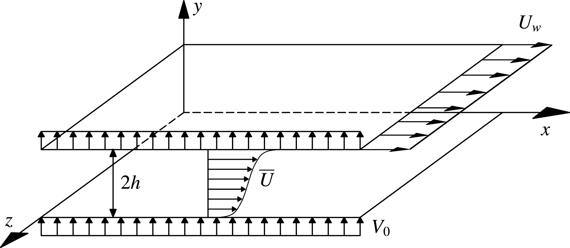
In this work, a new set of DNS of a plane CTF has been conducted within a computational box of $L_{x}=8\unicode[STIX]{x03C0}h$ , $L_{y}=2h$ and $L_{z}=3\unicode[STIX]{x03C0}h$ , with spanwise and streamwise periodicity (figure 1). In the past, this box has been used for very large turbulent Poiseuille flow simulations (Hoyas & Jiménez Reference Hoyas and Jiménez2006; Lee & Moser Reference Lee and Moser2015). However, it is known from the work by Avsarkisov et al. (Reference Avsarkisov, Hoyas, Oberlack and García-Galache2014a ) that this computational box might be too narrow and short to adequately reproduce a turbulent Couette flow. It was confirmed in Pirozzoli et al. (Reference Pirozzoli, Bernardini and Orlandi2014) that for pure Couette flow the correlation length in the spanwise direction is nominally infinity. In the case of the streamwise correlation length, we are interested in investigating if the transpiration velocity is capable of breaking down the large streamwise rolls appearing in classical Couette flows. Thus, the size of the box is a compromise between the capacity of running enough parametric cases and a large enough box to capture some of the largest scales of the flow.

The streamwise, wall-normal, and spanwise coordinates are $x,y$ and $z$ and the corresponding velocity components are $U,V$ and $W$ or, using index notation, $U_{i}$ . Statistically averaged quantities are denoted by an overbar, whereas fluctuating quantities are denoted by lowercase letters, i.e.  $U=\overline{U}+u$ . The flow is driven by a constant velocity of the upper wall such that we have the boundary condition $U(x,0,z)=0$ and $U(x,2h,z)=U_{w}$ . The blowing–suction process is implemented through the following boundary condition at the wall,

(2.1) $$\begin{eqnarray}\displaystyle V(x,0,z)=V(x,2h,z)=V_{0}, & & \displaystyle\end{eqnarray}$$

where $V_{0}$ is the constant transpiration velocity. The nominal Reynolds numbers studied are $Re_{\unicode[STIX]{x1D70F}}=250$ , 500 and 1000, based on the mean friction velocity $u_{\unicode[STIX]{x1D70F}}$ , the viscosity $\unicode[STIX]{x1D708}$ and on the channel half-width $h$ . In all cases the mass flow, and simultaneously the bulk velocity, $U_{b}$ , is kept constant, similar to Hoyas & Jiménez (Reference Hoyas and Jiménez2006), Avsarkisov et al. (Reference Avsarkisov, Hoyas, Oberlack and García-Galache2014a ). The mean friction velocity is defined as

(2.2) $$\begin{eqnarray}\displaystyle u_{\unicode[STIX]{x1D70F}}=\sqrt{\frac{(u_{\unicode[STIX]{x1D70F}}^{b})^{2}+(u_{\unicode[STIX]{x1D70F}}^{s})^{2}}{2}}, & & \displaystyle\end{eqnarray}$$

where the local friction velocities are

(2.3a,b ) $$\begin{eqnarray}\displaystyle u_{\unicode[STIX]{x1D70F}}^{b}=\sqrt{\unicode[STIX]{x1D708}|\unicode[STIX]{x2202}_{y}\overline{U}|_{b}},\quad u_{\unicode[STIX]{x1D70F}}^{s}=\sqrt{\unicode[STIX]{x1D708}|\unicode[STIX]{x2202}_{y}\overline{U}|_{s}}. & & \displaystyle\end{eqnarray}$$

Here and subsequently, superscripts $b$ and $s$ correspond to variables taken on the blowing and the suction side, respectively.

Figure 1.

Schematic view of Couette flow with moving wall velocity $U_{w}$ and wall-normal transpiration velocity $V_{0}$ . Fluid is blown through the lower wall and removed from the upper wall at a constant rate. The computational box is not scaled.

Table 1.

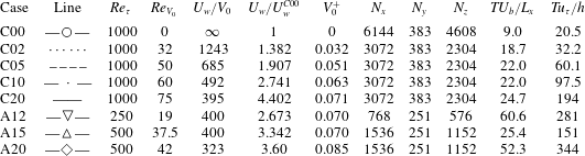
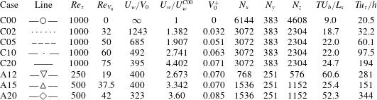
Parameters of the simulations. Three different Reynolds numbers are presented: $Re_{\unicode[STIX]{x1D70F}}$ is based on the mean friction velocity and the channel half-width $h$ and $Re_{V_{0}}$ is based on the transpiration velocity $V_{0}$ and $h$ . The third column, $U_{w}/V_{0}$ , is the ratio between the velocity of the wall $U_{w}$ and $V_{0}$ , which defines a Reynolds number usually employed for TASBL, see Bobke et al. (Reference Bobke, Örlü and Schlatter2015). Next, the velocities $U_{w}$ and $V_{0}$ are given in terms of the wall velocity of the pure Couette case, $U_{w}^{C00}$ , and the mean friction velocity $u_{\unicode[STIX]{x1D70F}}$ , respectively. $N_{x},N_{y},N_{z}$ are the numbers of collocation points. The last two columns denote the computational time span while statistics were taken in washouts ( $U_{b}/L_{x}$ ) and eddy turnovers ( $u_{\unicode[STIX]{x1D70F}}/h$ ).  $T$ is the computational time spanned by those fields. Line shapes given in the second column are used to identify the cases through all the figures of the present paper.

The Navier–Stokes equations, employed to investigate the present flow, are transformed into an equation for wall-normal vorticity $\unicode[STIX]{x1D714}_{y}$ and for the Laplacian of the wall-normal velocity $\unicode[STIX]{x1D719}=\unicode[STIX]{x1D6FB}^{2}v$ as in (Kim et al. Reference Kim, Moin and Moser1987). The spatial discretization uses dealiased Fourier expansions in the $x$ - and $z$ -directions, and seven-point compact finite differences in the $y$ -direction with fourth-order consistency and extended spectral-like resolution (Lele Reference Lele1992). The temporal discretization is a third-order semi-implicit Runge–Kutta scheme (Spalart Reference Spalart1991). Initial fields were either taken from previously calculated classical Couette flows imposing the new boundary conditions, or by further increasing the transpiration velocities in previously computed CTF cases.

Due to the lack of experimental data or numerical simulations, it has been impossible to do a formal validation of the code. However, in the past the code has been employed to successfully run simulations of turbulent Poiseuille flows (Hoyas & Jiménez Reference Hoyas and Jiménez2006; Hoyas & Jiménez Reference Hoyas and Jiménez2008), turbulent Couette flows (Avsarkisov et al. Reference Avsarkisov, Hoyas, Oberlack and García-Galache2014a ) and turbulent PTF (Avsarkisov et al. Reference Avsarkisov, Oberlack and Hoyas2014b ), while the modifications in the code to impose the new boundary conditions have been minimal. In addition, simulations conducted at very low transpiration velocity were similar to pure Couette flows. A comparison with the laminar solution, which can be derived analytically in form of an exponential function, and a comparison with the first $Re_{\unicode[STIX]{x1D70F}}=1000$ simulation reported (Pirozzoli et al. 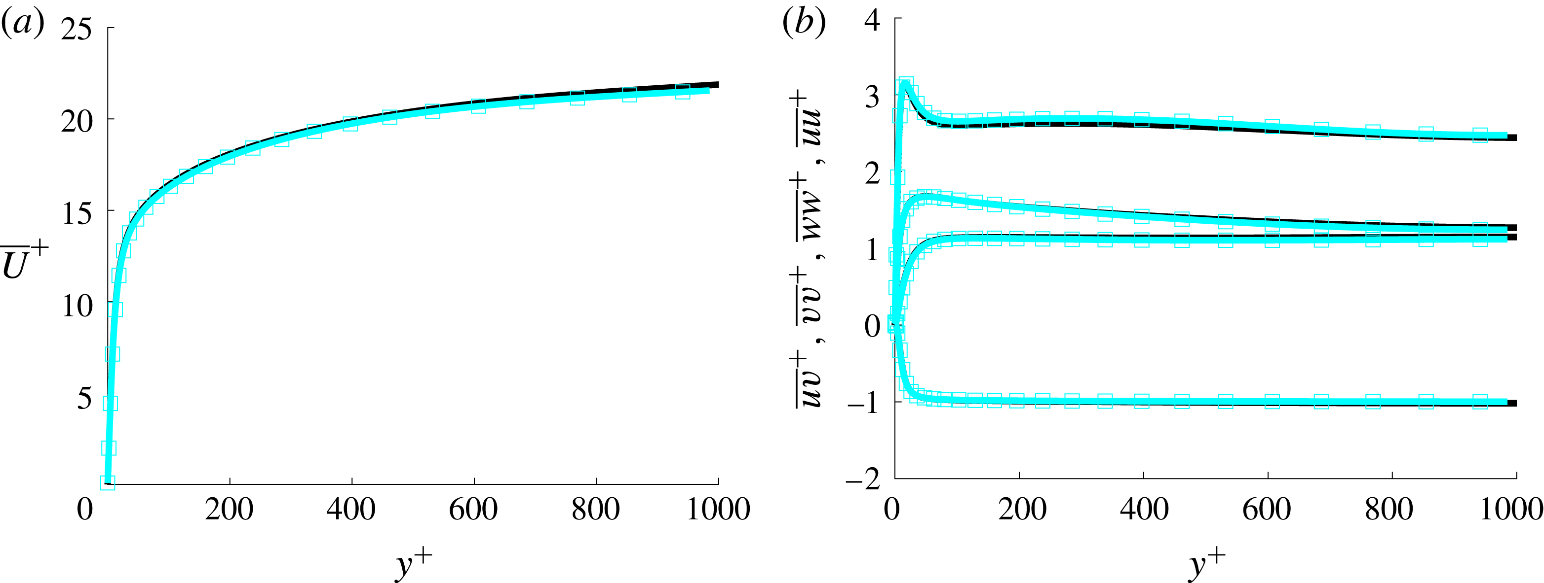Reference Pirozzoli, Bernardini and Orlandi2014) has been performed. Tests show a perfect agreement between DNS data and the analytic solution, though these results are omitted for brevity. The comparison of the present case C00 (explained below) with Pirozzoli et al.’s simulation is shown in figure 2. The agreement is excellent, both for the average velocity and the turbulent intensities.

Figure 2.

Mean velocity profile (a) and Reynolds stresses (b) scaled in inner scales ( $u_{\unicode[STIX]{x1D70F}},^{+}$ ). Black line, case C00 in table 1. Blue squares from Pirozzoli et al. (Reference Pirozzoli, Bernardini and Orlandi2014). Only half of the channel is shown.

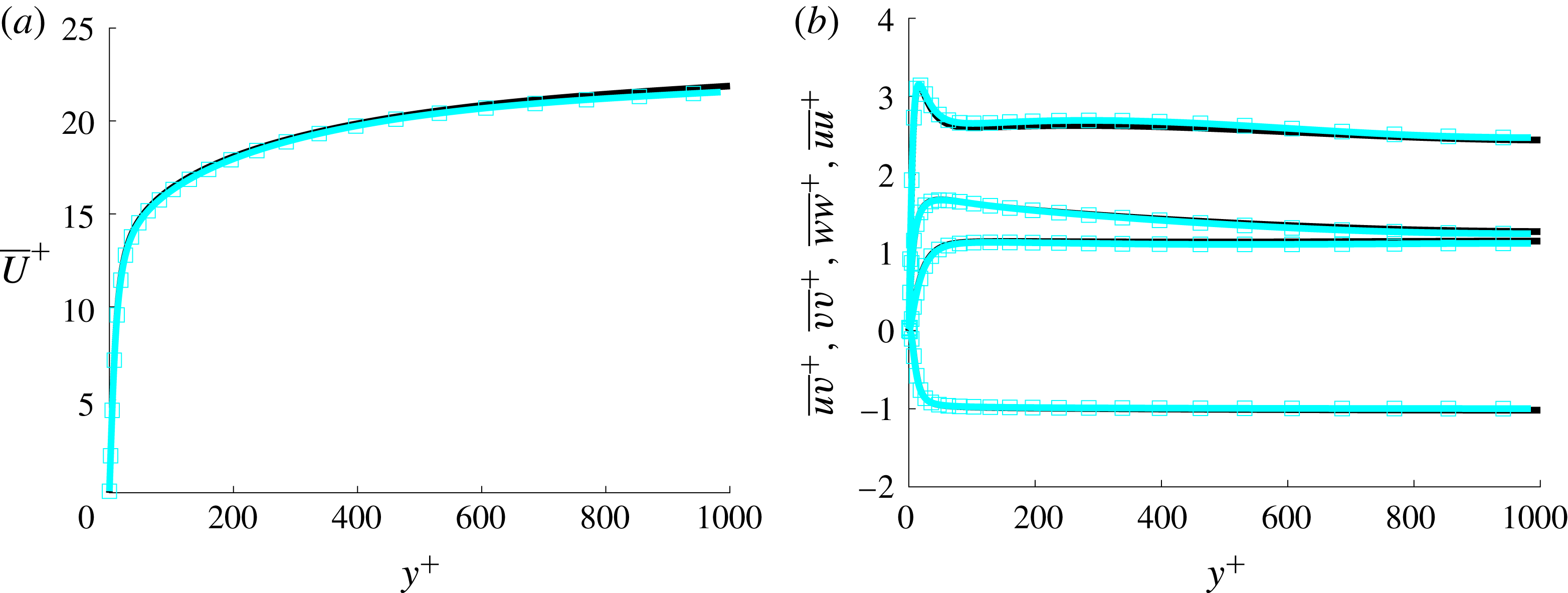
Table 1 summarizes the parameters of the present simulations. The wall-normal grid spacing is adjusted to keep the resolution at $\unicode[STIX]{x0394}y=1.5\unicode[STIX]{x1D702}$ , i.e., approximately constant in terms of the local isotropic Kolmogorov scale $\unicode[STIX]{x1D702}=(\unicode[STIX]{x1D708}^{3}/\unicode[STIX]{x1D716})^{1/4}$ for every $Re_{\unicode[STIX]{x1D70F}}$ case. In wall units, $\unicode[STIX]{x0394}y^{+}$ varies from $0.42$ at the wall up to $\unicode[STIX]{x0394}y^{+}\simeq 7.2$ at the centreline. The wall-parallel resolution in Fourier space for $x$ and $z$ is $\unicode[STIX]{x0394}x^{+}\simeq 12.2$ and $\unicode[STIX]{x0394}z^{+}\simeq 6.13$ . The case C00 is a pure turbulent Couette flow in a $16\unicode[STIX]{x03C0}h\times 2h\times 6\unicode[STIX]{x03C0}h$ computational box used as a reference case. The transpiration velocity grows for the cases C02 to C20. Cases A15 and A12 were ran to study the effect of increasing $Re_{\unicode[STIX]{x1D70F}}$ while keeping the dimensionless parameters $U_{w}/V_{0}$ and $V_{0}^{+}$ approximately constant. Case A20 was employed to see the effects of a higher transpiration rate at a lower Reynolds number.

In every simulation, the flow had to evolve from an initial file, which has been taken from previous different simulations. The code was run until a transition phase was passed and the flow had adjusted to the new set of parameters. The transition phase until the simulations reached a statistically steady state, which can be very time consuming, is not contemplated in the two right-hand columns of table 1. One of the measures used to assess that the code has run enough time to compile accurate statistics is to compute the total shear stress, which for the CTF reads

(2.4) $$\begin{eqnarray}\displaystyle \unicode[STIX]{x1D70F}_{b}+V_{0}\bar{U}=\unicode[STIX]{x1D708}\frac{\text{d}\bar{U}}{\text{d}y}-\overline{uv}, & & \displaystyle\end{eqnarray}$$

and, non-dimensionalized by $u_{\unicode[STIX]{x1D70F}}^{b}$ , yields

(2.5) $$\begin{eqnarray}\displaystyle 1+V_{0}^{+b}\bar{U}^{+b}-\frac{\text{d}\bar{U}^{+b}}{\text{d}y^{+b}}+\overline{uv}^{+b}=0. & & \displaystyle\end{eqnarray}$$

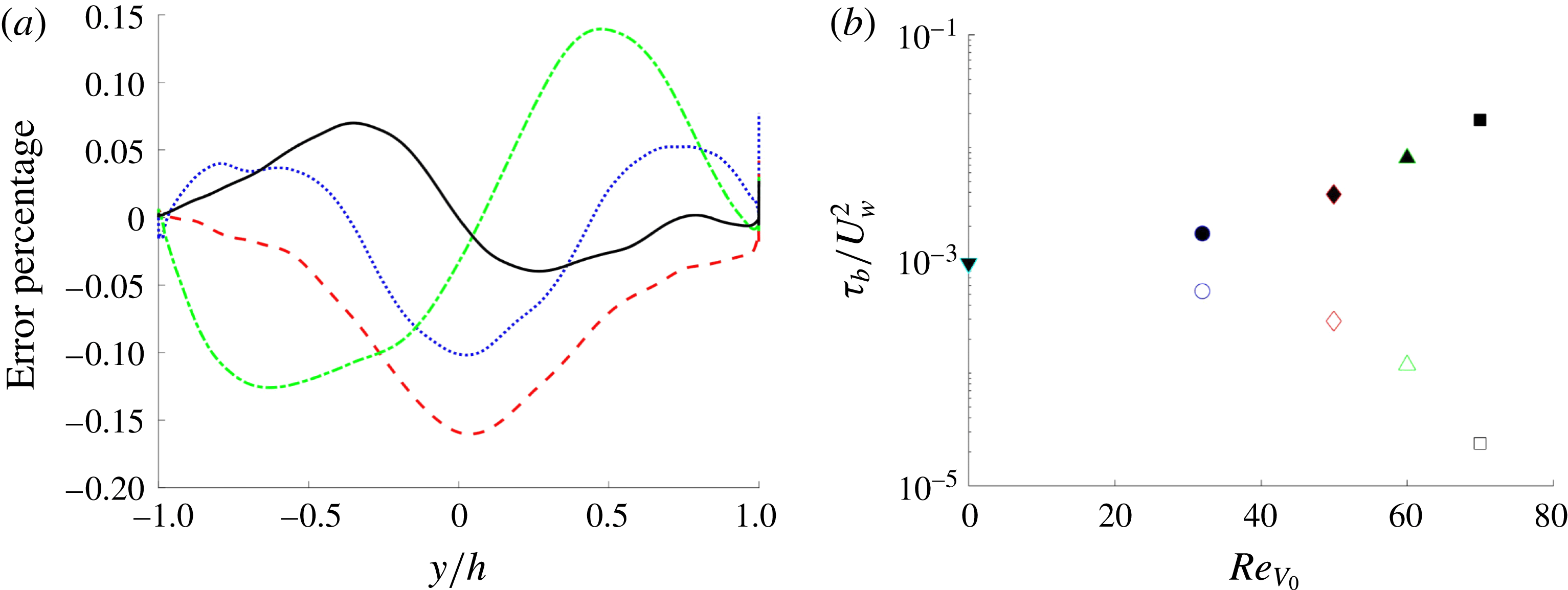
For the most unfavourable cases, i.e. $Re_{\unicode[STIX]{x1D70F}}=1000$ , the verification of (2.4) can be seen in figure 3(a), where the deviation from 0 of the left hand side of (2.5) has been plotted versus $y$ . As some of the terms of this equation can be large, the error has been normalized by the absolute maximum value of the terms presented in (2.5). The deviation in all cases is less than 0.15 % of the maximum value. It is worth noting that the transpiration velocity strongly modifies the shear stress at the wall, reducing it at the blowing wall and increasing it at the suction wall, as seen in figure 3(b). This modification of the value of $\unicode[STIX]{x1D70F}_{b}$ can be up to two orders of magnitude in the cases simulated.

Another important consequence of (2.4) is that, evaluating it at the upper wall and employing equation (2.3), we obtain

(2.6) $$\begin{eqnarray}\displaystyle (u_{\unicode[STIX]{x1D70F}}^{s})^{2}-(u_{\unicode[STIX]{x1D70F}}^{b})^{2}=V_{0}U_{w}, & & \displaystyle\end{eqnarray}$$

linking friction velocities with the value of the transpiration and the moving wall velocity.

Equation (2.6) has a strong effect in the developing processes of the flow once a new simulation is started. To run a simulation at a larger $Re_{V_{0}}$ , a field at smaller $Re_{V_{0}}$ is chosen. Thus the relationship between the local friction velocities changes, and consequently the global $Re_{\unicode[STIX]{x1D70F}}$ . In turn, it is necessary to change both the $Re_{U_{b}}$ and the wall velocity after a few hundred steps to obtain the desired value of the parameters. A second option would have been to increase $Re_{U_{b}}$ , but this option was discarded because the appropriate mesh size changed considerably.

In the present study we restrict ourselves to describing the new data coming from these simulations and comparing them with the results obtained for the pure Couette flow and other flows with wall transpiration, pointing out the key differences.

Figure 3.

Lines as in table 1. The suction wall is on the right of the figure. (a) Deviation of (2.5) from zero given in error percentage of the computation of the transpiration CXX cases. (b) Total shear stress $\unicode[STIX]{x1D70F}_{b}$ at the blowing (open symbols) and suction (closed symbols) walls for the different CXX cases.

3 Statistics

3.1 Mean velocity profile

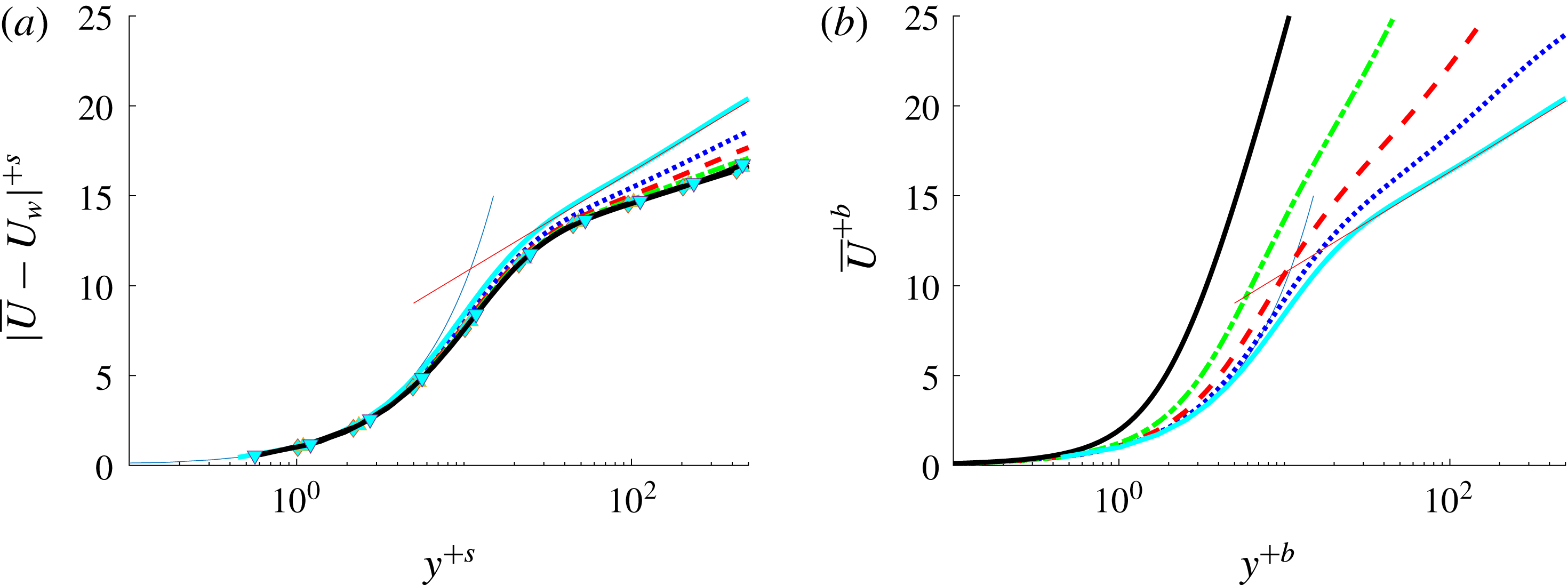
Figure 4 shows $\overline{U}$ at the suction and blowing sides scaled by the local $u_{\unicode[STIX]{x1D70F}}$ . At the suction wall the flow appears to follow the linear law in the viscous sublayer. However, at the blowing wall the interval where the linear law holds is shorter than the one near the suction side, and it gets further reduced as the transpiration number is increased. In the same figure, the red solid line shows the logarithmic profile,

(3.1) $$\begin{eqnarray}\displaystyle \overline{U}=\frac{1}{\unicode[STIX]{x1D705}}\ln y^{+}+B & & \displaystyle\end{eqnarray}$$

at the classical coefficient values of $\unicode[STIX]{x1D705}=0.41$ and $B=5.1$ (Pope Reference Pope2000). Qualitatively, the deviation from this logarithmic profile is in accordance with Sumitani & Kasagi (Reference Sumitani and Kasagi1995) and Kametani et al. (Reference Kametani, Fukagata, Örlü and Schlatter2015). This change in the slope seems to stop when $V_{0}^{+}$ is larger than 0.07 approximately, corresponding to $U_{\infty }/V_{0}\leqslant 400$ . 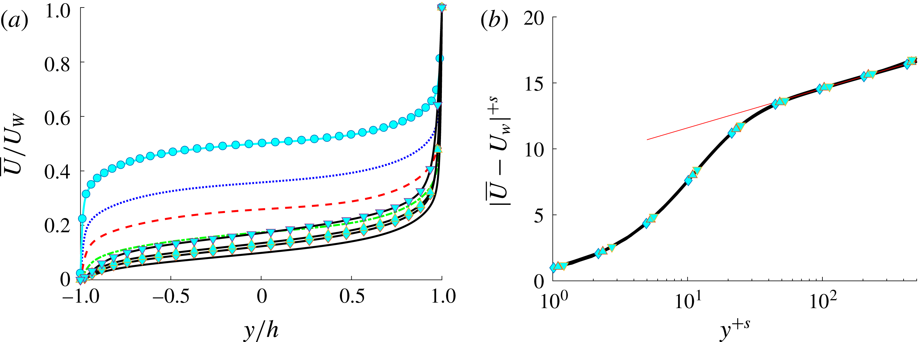Figure 5(b) shows $\overline{U}$ for the C20 and all A cases compared to a modified log law with $\unicode[STIX]{x1D705}=0.77$ and $B=8.7$ , with an excellent agreement.

Figure 4.

Lines as in table 1. Mean velocity profile scaled in inner local scales at the suction (a) and blowing (b) sides. Blue thin solid line corresponds to viscous sublayer linear scaling law; red thin solid line represents near-wall classical logarithmic scaling law at $\unicode[STIX]{x1D705}=0.41$ and $B=5.1$ .

Figure 5.

Lines as in table 1. (a) Mean velocity profile scaled in outer scales ( $U_{w},h$ ). (b) Mean velocity profile at the suction side scaled in $u_{\unicode[STIX]{x1D70F}}^{s}$ . Cases plotted: C20, A12, A15 and A20. Red thin solid line represents a modified logarithmic scaling law for $\unicode[STIX]{x1D705}=0.77$ and $B=8.7$ .

Figure 6.

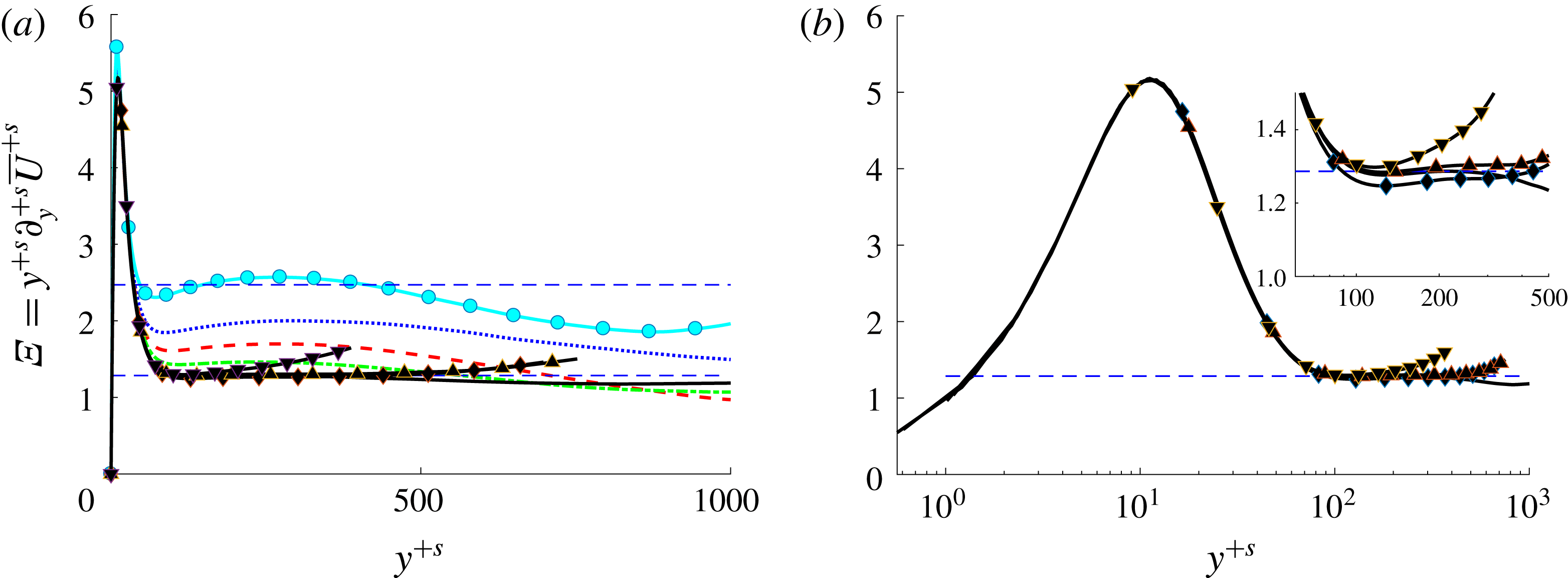
Lines as in table 1. Indicator function for the logarithmic layer, i.e. the inverse of the von Kármán constant scaled with $u_{\unicode[STIX]{x1D70F}}^{s}$ , (a) with dashed lines at $\unicode[STIX]{x1D705}=0.41$ and $\unicode[STIX]{x1D705}=0.77$ , (b) in semilogarithmic plot. Suction wall is at the left side of the plots.

However, using large eddy simulation (LES), Schlatter & Örlü (Reference Schlatter and Örlü2011) gave a value of $\unicode[STIX]{x1D705}=0.82$ and $B=9.2$ for a TASBL, independent of both $U_{\infty }/V_{0}$ and $Re_{\unicode[STIX]{x1D70F}}$ numbers. Further, Bobke et al. (Reference Bobke, Örlü and Schlatter2015) observed $\unicode[STIX]{x1D705}=0.89$ and $B=9.6$ for a TASBL at $U_{\infty }/V_{0}=333$ . It is clear from figure 4(a) that the slope of $\overline{U}$ changes with $U_{\infty }/V_{0}$ .

From a global point of view, the effect of the transpiration velocity in the mean velocity profiles may be taken from figure 5(a). This figure shows how transpiration leads to the loss of symmetry even for small $V_{0}^{+}$ , leading to higher mean velocity gradients at the suction wall and lower gradients at the blowing wall.

Figure 6 shows the mean velocity profile in terms of the inverse of the Kármán constant $1/\unicode[STIX]{x1D705}=y^{+s}\unicode[STIX]{x2202}U^{+s}/\unicode[STIX]{x2202}y^{+s}=\unicode[STIX]{x1D6EF}$ , which is the definition of the log indicator function. Apparently, with increasing transpiration rate, the region where this term is almost constant increases drastically. In fact, for the highest transpiration rate presented here, an approximately constant region between $y^{+s}=80$ and $y^{+s}=1000$ can be observed. This flattening effect is related to the vanishing of the secondary maximum that exists at approximately $y^{+}=300$ for the C00 case. The value of the log indicator function $\unicode[STIX]{x1D6EF}$ for the second set of simulations (C20, A20, A15 and A12) can be seen in the semilogarithmic representation in figure 6(b). There is a perfect collapse of the data below the logarithmic layer, i.e. in the viscous sublayer and the buffer layer, as the lower-Reynolds-number cases AXX collapse onto the $Re_{\unicode[STIX]{x1D70F}}=1000$ curve (cases CXX). All cases present a similarly extended region, and in the range of transpiration numbers studied, this seems to be an intermediate limit. The existence of a displaced secondary maximum or minimum can be discarded in the range of the presently studied parameters.

One of the possible reasons for the greatly extended range of validity of the log-region might be the value of $u_{\unicode[STIX]{x1D70F}}^{s}$ which is ten times larger than the one for the classical Couette flow. As will be shown later, this effect can also be tentatively linked to the size and structure of the eddies present in the flow.

Figure 7.

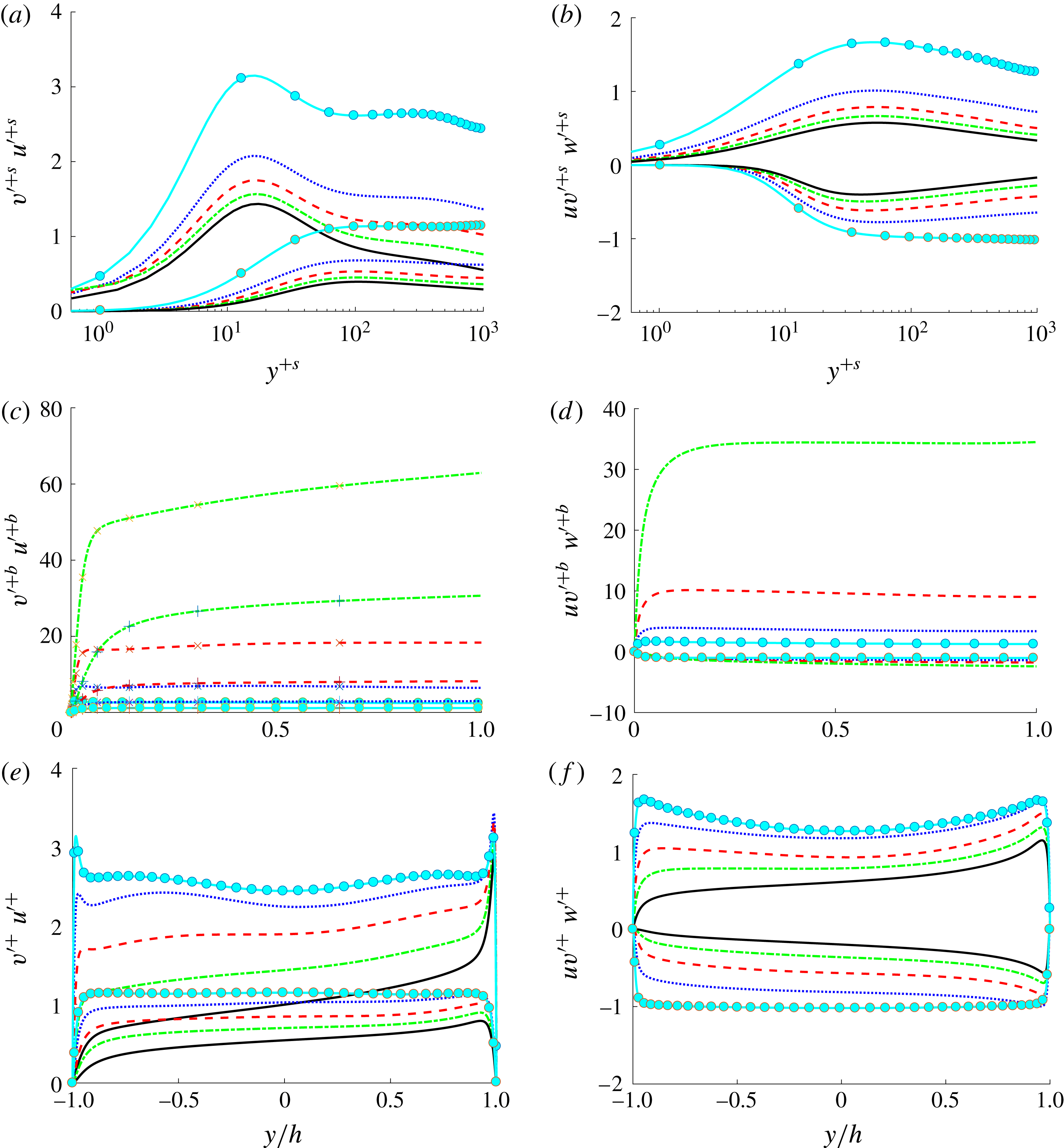
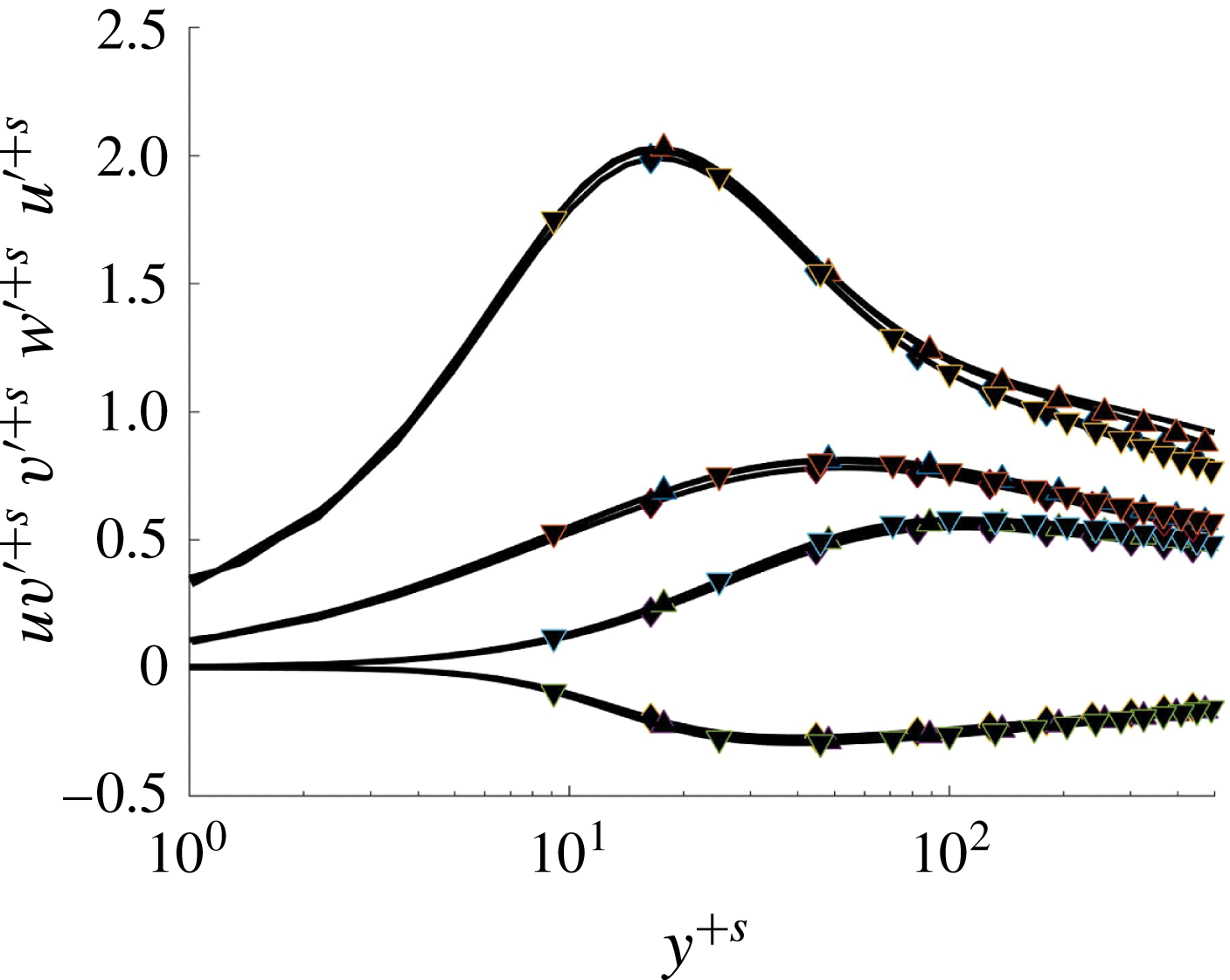
Lines as in table 1. Velocity fluctuation intensities of the CXX cases. (a,c,e) $u^{\prime }$ and $v^{\prime }$ ; (b,d,f) $w^{\prime }$ and $\overline{uv}$ . (a,b) Adimensionalized by $u_{\unicode[STIX]{x1D70F}}^{s}$ , plotted versus dimensionless distance from the suction wall in local inner units, $y^{+s}=(2-y/h)u_{\unicode[STIX]{x1D70F}}^{s}/\unicode[STIX]{x1D708}$ . (c,d) Adimensionalized by $u_{\unicode[STIX]{x1D70F}}^{b}$ , plotted versus distance from blowing wall in outer units. (e,f) Adimensionalized by $u_{\unicode[STIX]{x1D70F}}$ , plotted versus distance from blowing wall in outer units.

3.2 Turbulent intensities

In figure 7, the root-mean-square velocity fluctuations ${u_{i}^{\prime }}^{+}=(\overline{u_{[i]}u_{[i]}}^{\,+})^{1/2}$ , where index in brackets denote no summation, and $u{v^{\prime }}^{+}=\overline{uv}^{+}$ are presented for the different transpiration cases to be also compared to the pure Couette case. As for the mean velocity $\overline{U}$ , the scaling with a local $u_{\unicode[STIX]{x1D70F}}$ does not collapse the data.

It should be mentioned that normalization is not trivial here, since there are several velocity scales acting on the flow. Through the boundary conditions we have the external scales $U_{w}$ and $V_{0}$ , while internally we have the two friction velocities defined in (2.3), which are all related through the global momentum balance in (2.6). As was observed in previous works investigating the TASBL (Sumitani & Kasagi Reference Sumitani and Kasagi1995; Schlatter & Örlü Reference Schlatter and Örlü2011; Bobke et al. Reference Bobke, Örlü and Schlatter2015; Kametani et al. Reference Kametani, Fukagata, Örlü and Schlatter2015), we analogously find that by scaling with the local friction velocity, the turbulent intensities get reduced at the suction wall and increased near the blowing wall. Further, the known peaks of ${u_{i}^{\prime }}^{+}$ and ${w_{i}^{\prime }}^{+}$ (Hoyas & Jiménez Reference Hoyas and Jiménez2006; Avsarkisov et al. Reference Avsarkisov, Oberlack and Hoyas2014b ) disappear at the blowing wall.

The situation when keeping the transpiration rate constant, while at the same time varying the Reynolds number, i.e. comparing the C20 case and all AXX cases, is depicted in figure 8. In this context, at the suction wall the local friction velocity $u_{\unicode[STIX]{x1D70F}}^{s}$ seems to be the most appropriate scaling, as it nicely collapses the data. However, this scaling, using $u_{\unicode[STIX]{x1D70F}}^{b}$ , fails completely at the suction wall (not shown). This failure is apparently a consequence of the term $V_{0}U_{w}$ in the momentum conservation equation (2.4), as the product $U_{w}^{+}V_{0}^{+}$ is constant for the C20 and AXX cases. This obvious scaling problem near the suction side will be studied in a companion paper. To facilitate the visualization and the comparison between both walls, in most of the figures and discussion that follows, global wall units will be used.

Figure 8.

Lines as in table 1. Velocity fluctuation intensities of the AXX and C20 cases are plotted versus the dimensionless distance from the suction wall in local inner units.

3.3 Turbulent budgets

The budget equation for the Reynolds-stress-tensor components $\overline{u_{i}u_{j}}$ , is given by

(3.2) $$\begin{eqnarray}\displaystyle B_{ij}\equiv \frac{\text{D}\overline{u_{i}u_{j}}}{\text{D}t}=P_{ij}+\unicode[STIX]{x1D700}_{ij}+T_{ij}+\unicode[STIX]{x1D6F1}_{ij}^{s}+\unicode[STIX]{x1D6F1}_{ij}^{d}+V_{ij}, & & \displaystyle\end{eqnarray}$$

where $\text{D}/\text{D}t$ is the mean substantial derivative and $(u_{1},u_{2},u_{3})=(u,v,w)$ . The different terms on the right-hand side are referred to as production, dissipation, turbulent diffusion, pressure strain, pressure diffusion, and viscous diffusion, respectively. They are defined according to

(3.3a ) $$\begin{eqnarray}\displaystyle & \displaystyle P_{ij}=-\overline{u_{i}u_{k}}\unicode[STIX]{x2202}_{x_{k}}\overline{U}_{j}-\overline{u_{j}u_{k}}\unicode[STIX]{x2202}_{x_{k}}\overline{U}_{i}, & \displaystyle\end{eqnarray}$$

(3.3b ) $$\begin{eqnarray}\displaystyle & \displaystyle \unicode[STIX]{x1D700}_{ij}=-2\unicode[STIX]{x1D708}\overline{\unicode[STIX]{x2202}_{x_{k}}u_{i}\unicode[STIX]{x2202}_{x_{k}}u_{j}}, & \displaystyle\end{eqnarray}$$

(3.3c ) $$\begin{eqnarray}\displaystyle & \displaystyle T_{ij}=-\unicode[STIX]{x2202}_{x_{k}}\overline{u_{i}u_{j}u_{k}}, & \displaystyle\end{eqnarray}$$

(3.3d ) $$\begin{eqnarray}\displaystyle & \displaystyle \unicode[STIX]{x1D6F1}_{ij}^{s}=\overline{p(\unicode[STIX]{x2202}_{x_{j}}u_{i}+\unicode[STIX]{x2202}_{x_{i}}u_{j})}, & \displaystyle\end{eqnarray}$$

(3.3e ) $$\begin{eqnarray}\displaystyle & \displaystyle \unicode[STIX]{x1D6F1}_{ij}^{d}=-\unicode[STIX]{x2202}_{x_{k}}(\unicode[STIX]{x1D6FF}_{ki}\overline{pu_{j}}+\unicode[STIX]{x1D6FF}_{kj}\overline{pu_{i}}), & \displaystyle\end{eqnarray}$$

(3.3f ) $$\begin{eqnarray}\displaystyle & \displaystyle V_{ij}=\unicode[STIX]{x1D708}\unicode[STIX]{x2202}_{x_{k}}\unicode[STIX]{x2202}_{x_{k}}\overline{u_{i}u_{j}}. & \displaystyle\end{eqnarray}$$

In the previous definitions, $\unicode[STIX]{x1D6FF}_{ij}$ is Kronecker’s delta and repeated indices imply summation over $k=1,2,3$ . In canonical wall flows without wall transpiration (Hoyas & Jiménez Reference Hoyas and Jiménez2008; Avsarkisov et al. Reference Avsarkisov, Oberlack and Hoyas2014b ), $\text{D}\overline{u_{i}u_{j}}/\text{D}t$ is zero. However, as soon as $V_{0}$ is different from zero, the convective derivative in the $y$ -direction does not vanish. Hence, from the four terms, the only remaining one is

(3.4) $$\begin{eqnarray}\displaystyle B_{ij}=V_{0}\unicode[STIX]{x2202}_{x_{2}}\overline{u_{i}u_{j}}. & & \displaystyle\end{eqnarray}$$

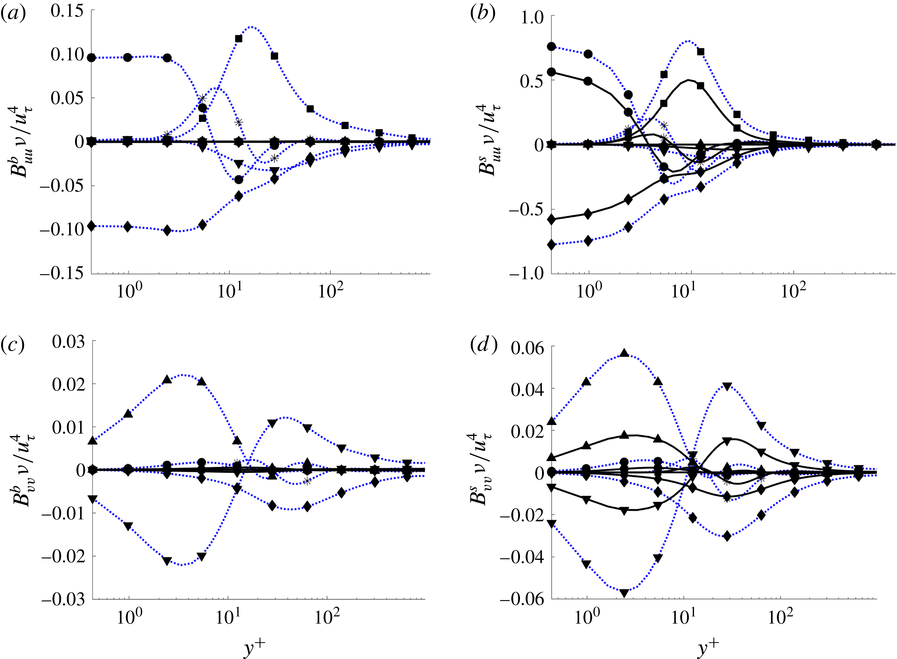
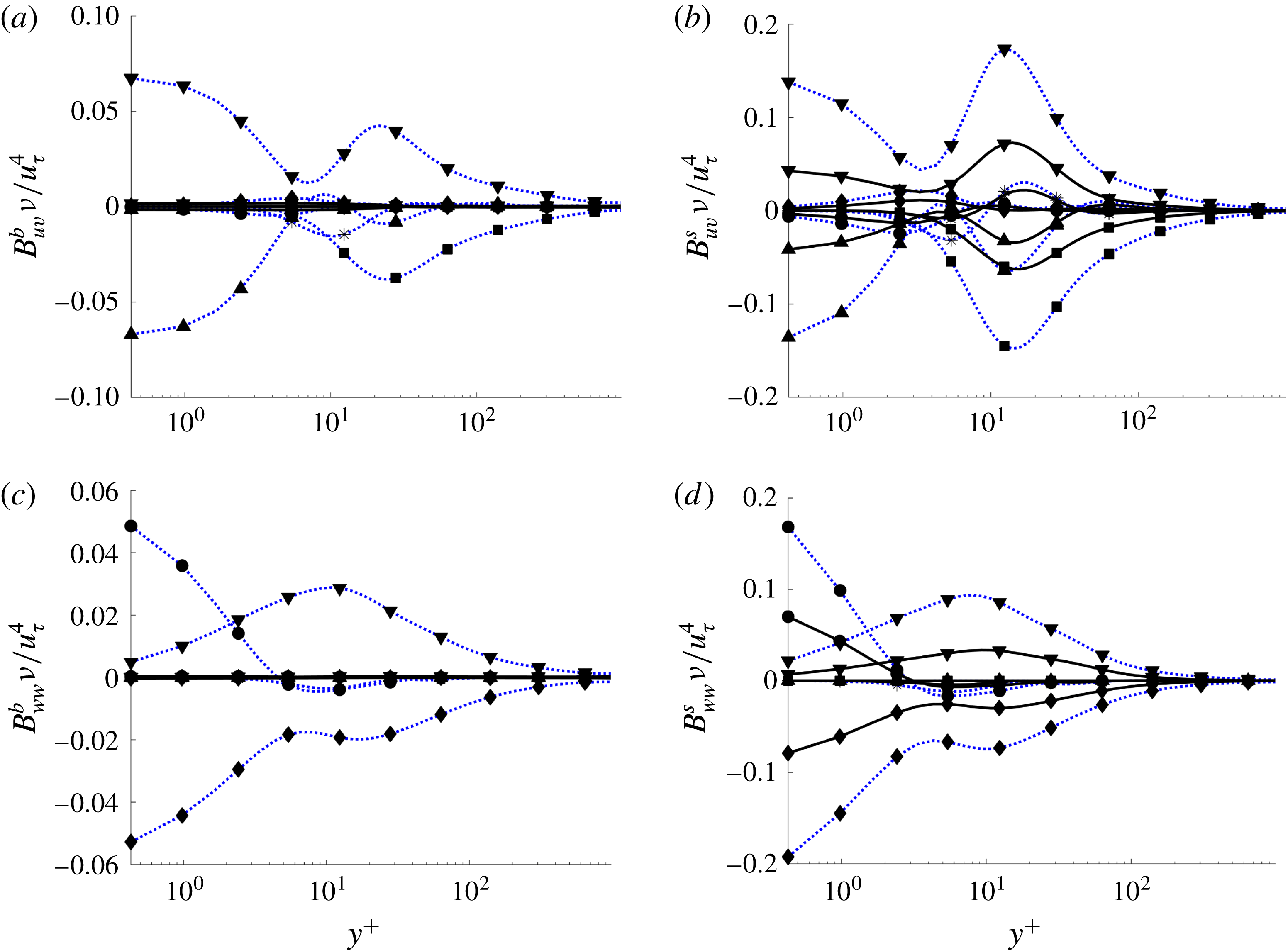
The four non-trivial budgets are shown in figures 9 and 10 non-dimensionalized by $\unicode[STIX]{x1D708}/u_{\unicode[STIX]{x1D70F}}^{4}$ . For the sake of clarity, only the cases C02 and C20 are plotted. The data from all the cases can be downloaded from our webpage given at the end of the abstract above. A general observation is that transpiration leads to a reduction of essentially all terms in the balance equation for $\overline{u_{i}u_{j}}$ in (3.2). Near the blowing wall, the values are several orders of magnitude smaller than at the suction wall. The peaks of the different quantities are in the same location as for the canonical flows (Hoyas & Jiménez Reference Hoyas and Jiménez2008). 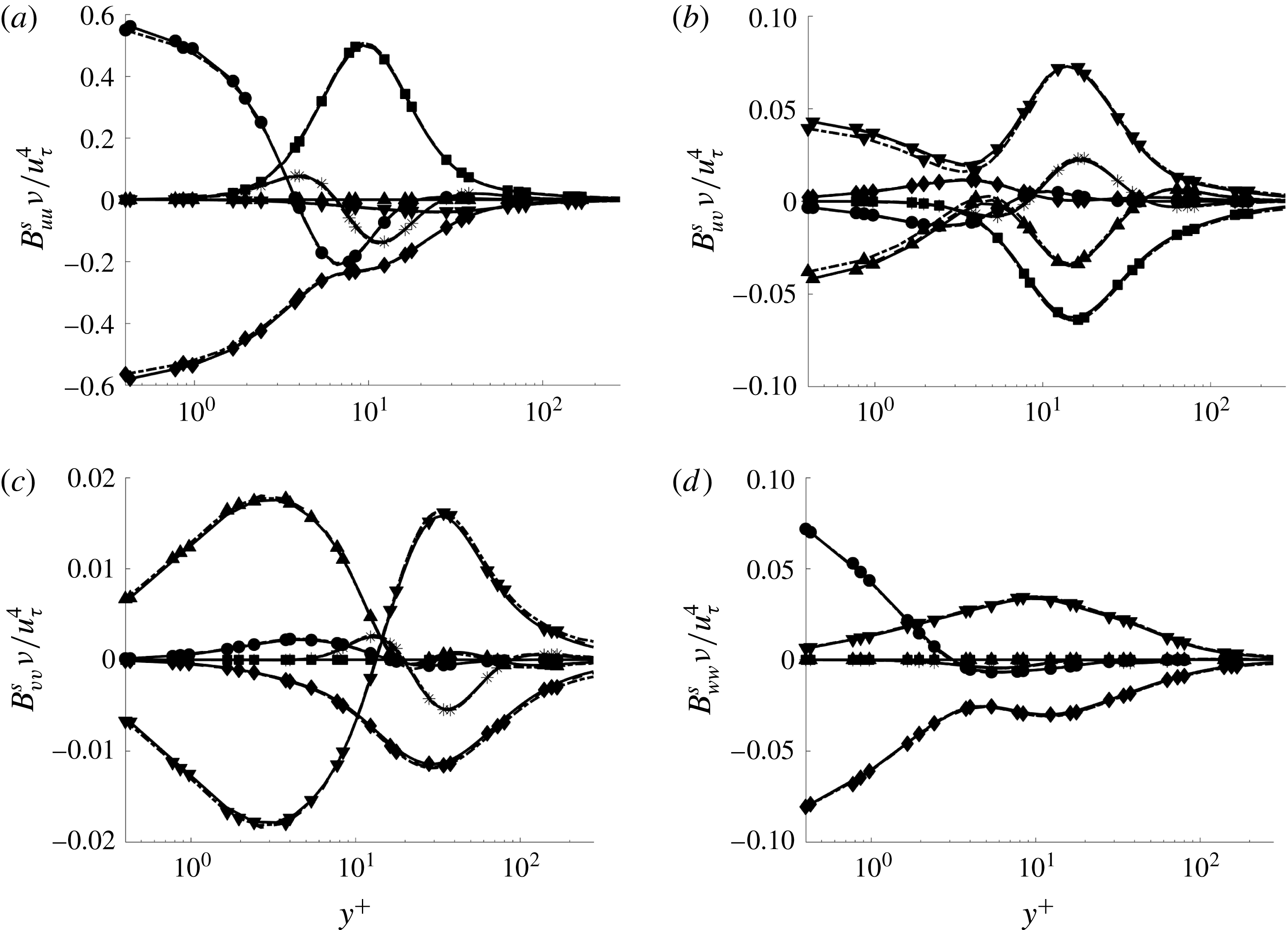In accordance to our observations for the turbulent intensities, $u_{\unicode[STIX]{x1D70F}}$ alone seems not to be sufficient to properly scale, i.e. collapse, the turbulent budget. However, studying a constant suction at varying Reynolds number, i.e. considering $V_{0}^{+}=0.07$ , the curves of the budgets $B_{uu}$ and $B_{ww}$ for the cases A12, A15 and C20 collapse onto one curve, as can be seen in figure 11. This clearly indicates that the value of $V_{0}^{+}$ is the key parameter for most of the turbulence properties.

Figure 9.

Budgets for Reynolds stresses $\overline{uu}$ and $\overline{vv}$ . Only Cases C02 and C20 are shown. (a) $B_{uu}$ , blowing side; (b) $B_{uu}$ , suction side; (c) $B_{vv}$ , blowing side; (d) $B_{vv}$ , suction side. Production ▪, dissipation ♦, viscous diffusion ●, pressure strain ▾, pressure diffusion ▴, turbulent diffusion *. Lines as in table 1.

Figure 10.

Budgets for Reynolds stresses $\overline{uv}$ and $\overline{ww}$ . Only Cases C02 and C20 are shown. (a) $B_{uv}$ , blowing side; (b) $B_{uv}$ , suction side; (c) $B_{ww}$ , blowing side; (d)  $B_{ww}$ , suction side. Production ▪, dissipation ♦, viscous diffusion ●, pressure strain ▾, pressure diffusion ▴, turbulent diffusion *. Lines as in table 1.

Figure 11.

Budgets for Reynolds stresses. Cases for $V_{0}^{+}=0.07$ at the suction side are shown. (a) $B_{uu}$ , (b) $B_{uv}$ , (c) $B_{ww}$ , (d) $B_{ww}$ . Production ▪, dissipation ♦, viscous diffusion ●, pressure strain ▾, pressure diffusion ▴, turbulent diffusion *. Lines differ from table 1: Case C20, solid. Case A15, dashed. Case A12, dash-dotted.

The data presented in this section are in agreement with several other works of Sumitani & Kasagi (Reference Sumitani and Kasagi1995), Kametani et al. (Reference Kametani, Fukagata, Örlü and Schlatter2015), Bobke et al. (Reference Bobke, Örlü and Schlatter2015), if the local friction velocity is used for scaling the flow. The values of the intensities increase near the blowing wall and decrease close to the suction side as expected. However, this effect is larger than in the flows studied previously. At the blowing wall, as the transpiration velocity increases, the value of $Re_{\unicode[STIX]{x1D70F}}^{b}$ gets reduced. For $V_{0}^{+}>0.06$ , the known peaks of the intensities of $u_{i}^{\prime +b}$ and $w_{i}^{\prime +b}$ disappear (see figure 7 c,d). In contrast to the previous works, the existence of the global $u_{\unicode[STIX]{x1D70F}}$ linking both walls can be used to analyse and compare the behaviour of the flow at both walls (see figure 7 e,f). This is not possible in TASBL flows as these experiments have only one type of permeable boundary condition. The damping of turbulence induced by the reduction of the local friction velocity at the blowing wall does not coincide with an increase of the turbulent budgets near the blowing wall when $V_{0}^{+}>0.06$ , as can be seen in figures 9 and 10. Turbulence is dampened in both walls if scaled in global wall units. In the following section, the turbulent structures created by the joint action of both walls will be analysed.

4 Turbulent structures

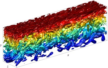
The one-point statistical study conducted in the previous section is complemented here with the analysis of the geometrical structures of the flow. Figure 12 shows the vortical structures for the case A12, computed using Hunt’s vortex criterion (Hunt, Wray & Moin Reference Hunt, Wray and Moin1988). This criterion is based on the second invariant of the velocity gradient tensor, $\unicode[STIX]{x1D64C}$ , defined as

(4.1) $$\begin{eqnarray}\displaystyle \unicode[STIX]{x1D64C}={\textstyle \frac{1}{2}}((\unicode[STIX]{x1D6FA}_{ii}^{2})^{1/2}-(\unicode[STIX]{x1D61A}_{ii}^{2})^{1/2}), & & \displaystyle\end{eqnarray}$$

where $\unicode[STIX]{x1D64E}$ and $\unicode[STIX]{x1D6FA}$ are the symmetric and antisymmetric parts of the gradient tensor,

(4.2a,b ) $$\begin{eqnarray}\displaystyle \unicode[STIX]{x1D61A}_{ij}={\textstyle \frac{1}{2}}(\unicode[STIX]{x2202}_{i}U_{j}+\unicode[STIX]{x2202}_{j}U_{i}),\quad \unicode[STIX]{x1D6FA}_{ij}={\textstyle \frac{1}{2}}(\unicode[STIX]{x2202}_{i}U_{j}-\unicode[STIX]{x2202}_{j}U_{i}) & & \displaystyle\end{eqnarray}$$

and $\unicode[STIX]{x1D61A}_{ii}^{2}=\unicode[STIX]{x1D61A}_{ij}\unicode[STIX]{x1D61A}_{ji}$ , $\unicode[STIX]{x1D6FA}_{ii}^{2}=\unicode[STIX]{x1D6FA}_{ij}\unicode[STIX]{x1D6FA}_{ji}$ . At each point a single value of $\unicode[STIX]{x1D64C}$ is calculated based on the velocity field. If this value of $\unicode[STIX]{x1D64C}$ is larger than a certain threshold, (Chakraborty, Balachandar & Adrian Reference Chakraborty, Balachandar and Adrian2005; del Álamo et al. Reference del Álamo, Jiménez, Zandonade and Moser2006) a vortical structure is detected. Using this method it is possible to define a map, $H(x,y,z)$ , such that

(4.3) $$\begin{eqnarray}\displaystyle H(x,y,z)=\left\{\begin{array}{@{}ll@{}}1 & \text{if }\text{Hunt's criterion is true,}\\ 0 & \text{elsewhere.}\end{array}\right. & & \displaystyle\end{eqnarray}$$

The methods by Jeong & Hussain (Reference Jeong and Hussain1995) and Chong, Perry & Cantwell (Reference Chong, Perry and Cantwell1990) were also implemented, but as the results of all three methods were similar, we only used Hunt’s criterion.

Figure 12.

Vortical structures for the A12 case, coloured by height. Only a fourth of the length in $x$ and an eighth in $z$ is shown.

Figure 13.

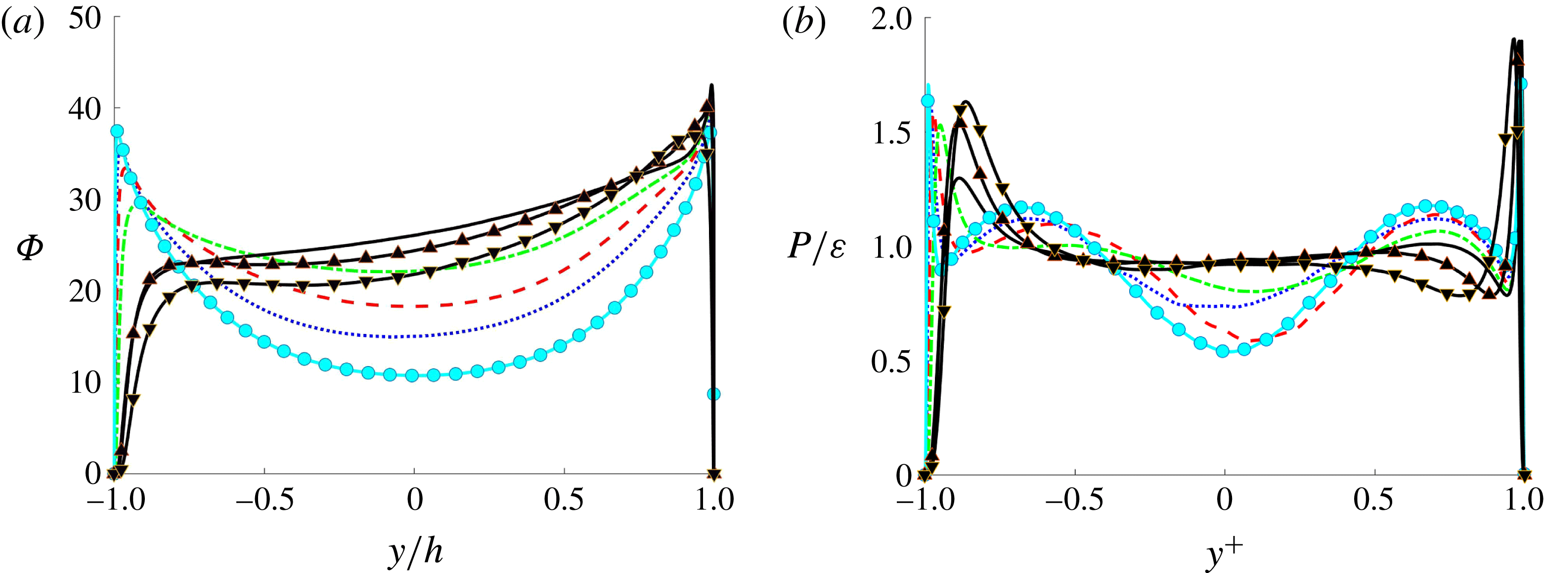
Lines as in table 1. (a) Percentage of points where Hunt’s criterion is positive. (b) Production to dissipation ratio.

It is clear from this figure that the structures at the blowing side are wider, larger and less frequent than those at the suction side. A statistical measure for the distribution of vortices is presented in figure 13(a). This figure shows the function $\unicode[STIX]{x1D6F7}$ , defined as

(4.4) $$\begin{eqnarray}\displaystyle \unicode[STIX]{x1D6F7}(y)=\mathop{\sum }_{x}\mathop{\sum }_{z}H(x,y,z)/(N_{x}\times N_{z})\times 100, & & \displaystyle\end{eqnarray}$$

i.e. for every plane $\unicode[STIX]{x1D6F7}(y)$ is the number of points where Hunt’s criterion is true over the total number of points. This quantifies the average area covered by eddies in the box. When the transpiration velocity is larger than a certain threshold, $\unicode[STIX]{x1D6F7}$ seems to converge to a linear function in the centre region of the channel. This is most clearly visible for the case C20. For the cases A12 and A15, $\unicode[STIX]{x1D6F7}$ still presents some curvature at the centre of the channel. The integral of $\unicode[STIX]{x1D6F7}$ ,

(4.5) $$\begin{eqnarray}\displaystyle V_{\unicode[STIX]{x1D6F7}}=\int _{-h}^{h}\unicode[STIX]{x1D6F7}\,\text{d}y, & & \displaystyle\end{eqnarray}$$

gives an estimation of the part of volume of the channel where a vortical structure exists. This volume grows from $V_{\unicode[STIX]{x1D6F7}}=34.25$ for the pure Couette flow to $V_{\unicode[STIX]{x1D6F7}}=53.12$ for the case C20. Hence, it indicates a greater percentage of vortices as the transpiration velocity is increased. Although the value of $\unicode[STIX]{x1D6F7}$ at the blowing wall is reduced as the transpiration is increased, the growth of $\unicode[STIX]{x1D6F7}$ at the centre of the channel compensates this decrease. Moreover, the values of $\unicode[STIX]{x1D6F7}$ for the case C20 in the outer region of the channel, i.e. 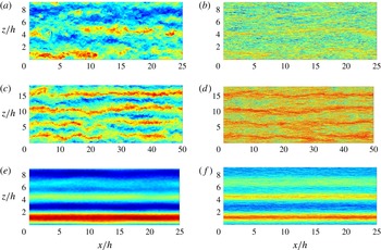from $h=-0.8$ to $h=0.8$ , lie in the range from $\unicode[STIX]{x1D6F7}=22$ to $\unicode[STIX]{x1D6F7}=34$ , which is approximately the range of values for $\unicode[STIX]{x1D6F7}$ in the logarithmic layer of the case C00. This corresponds to more ‘streaky’ flow structures which can be confirmed in figure 14. Here contours of the streamwise velocity in parallel planes to the wall are shown for the pure Couette flow, and instantaneous and ensemble-averaged values for the C20 case are presented at the centreline $y/h=0$ and at $y^{+}=10$ , where the latter is the position of the maximum of the production in figure 9(b).

Figure 14.

$U$ velocity coherent structures in $x$ – $z$ planes. (a,c,e) $y/h=0$ (centreline), (b,d,f) $y^{+}=10$ for the following cases: (a,b) C00, instantaneous field, (c,d) C20, instantaneous field, (e,f) C20, averaged.

As was expected from figure 13(a), it is clear that the density of vortices is larger in case C20 compared to case C00. A clear organization into high-speed (red) and low-speed (blue) streaks is observed. These streaks maintain some coherence along the whole channel. Case C20 shows a stronger organization of the flow than case C00 close to the suction wall. To investigate this further, the ratio of production to dissipation $P/\unicode[STIX]{x1D700}$ is shown in figure 13(b). Following the classical result from Lam & Banerjee (Reference Lam and Banerjee1992), streaks can only be sustained if $P/\unicode[STIX]{x1D700}$ is at least of order unity. This ratio is almost exactly unity for the case C20 case, and the cases A12 and A15 are more flat than any other case. 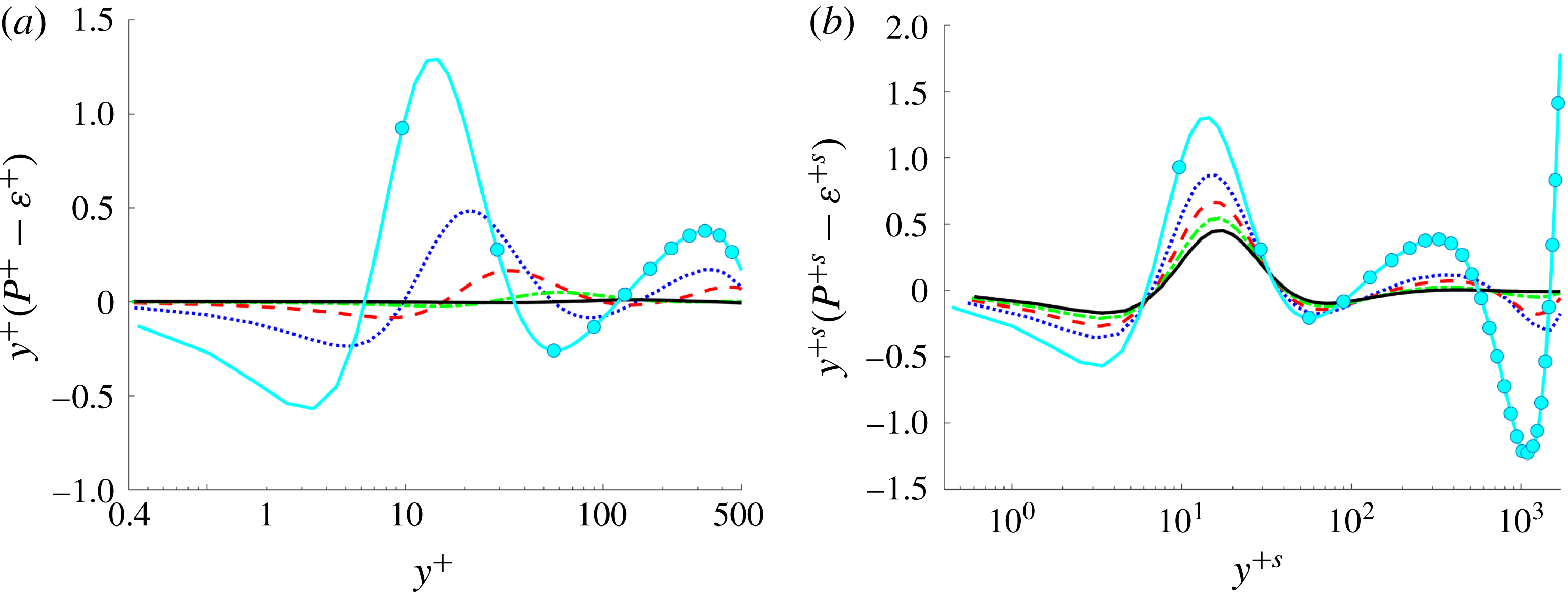The mechanisms triggering these two effects, linear decreasing of the area of eddies and $P/\unicode[STIX]{x1D700}=1$ could be the same which provoke the extremely long region where the indicator function is constant (see § 3.1). One of the arguments in favour of this can be seen in figure 16. Herein, the local excess of $P$ over $\unicode[STIX]{x1D700}$ is plotted, though premultiplied by $y^{+}$ , so that equal areas below the curve correspond to equal contributions. Pirozzoli et al. (Reference Pirozzoli, Bernardini and Orlandi2011) argue that the excess of production over dissipation around the secondary peak of $y^{+}(P-\unicode[STIX]{x1D700})$ at $y^{+}\approx 400$ has to be transferred towards the underlying layers. This secondary peak is dampened as the transpiration velocity is increased. For the case C20 there is no excess of production (or dissipation) for almost the entire core of the channel (see figure 13 b).

Figure 15.

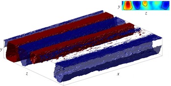
Coherent structures obtained from the ensemble average of the flow field spanning through all the channel length for the C20 case. Only a half of the length in $x$ is shown.

Figure 16.

Distribution of premultiplied turbulence kinetic energy production excess at the blowing (a) and suction wall (b). Lines as in table 1.

A second point of view refers to the very long and wide structures in classical Couette flows (Tsukahara et al. Reference Tsukahara, Kawamura and Shingai2006; Kitoh & Umeki Reference Kitoh and Umeki2008; Avsarkisov et al. Reference Avsarkisov, Hoyas, Oberlack and García-Galache2014a ; Pirozzoli et al. Reference Pirozzoli, Bernardini and Orlandi2014), which can be as long as $310h$ for $Re_{\unicode[STIX]{x1D70F}}=500$ , Lee & Moser (Reference Lee and Moser2017). As Pirozzoli et al. (Reference Pirozzoli, Bernardini and Orlandi2014) indicates, the streaks with a spanwise length of $2h$ basically have an infinite correlation length. This kind of structure has been linked to a quasiperiodic process (Hamilton, Kim & Waleffe Reference Hamilton, Kim and Waleffe1995). In the core region of a turbulent plane Couette flow, low-velocity streaks generate large-scale vortices. The existence of such a regeneration mechanism in the core region was confirmed experimentally by Kitoh & Umeki (Reference Kitoh and Umeki2008) and numerically by Pirozzoli et al. (Reference Pirozzoli, Bernardini and Orlandi2011) and Pirozzoli et al. (Reference Pirozzoli, Bernardini and Orlandi2014). This process does not occur in turbulent Poiseuille flows. Our observations may indicate that the presence of transpiration is not, in all the cases we have studied, able to completely break this mechanism. After averaging the streamwise velocity for 24.7 washouts, the rolls are still present, as can be seen in figure 14(e,f). This phenomenon can be appreciated in figure 15, where we show the different pairs of counter-rotating rolls whose footprints are shown in figure 14(e,f). The contour level of these rolls can be observed in the upper right corner of figure 15. This subplot shows different contour levels for the mean in $x$ of the ensemble average of $U$ . It is clear that some pairs of rolls are stronger than others, differently from Avsarkisov et al. (Reference Avsarkisov, Hoyas, Oberlack and García-Galache2014a ), but they are undoubtedly present.

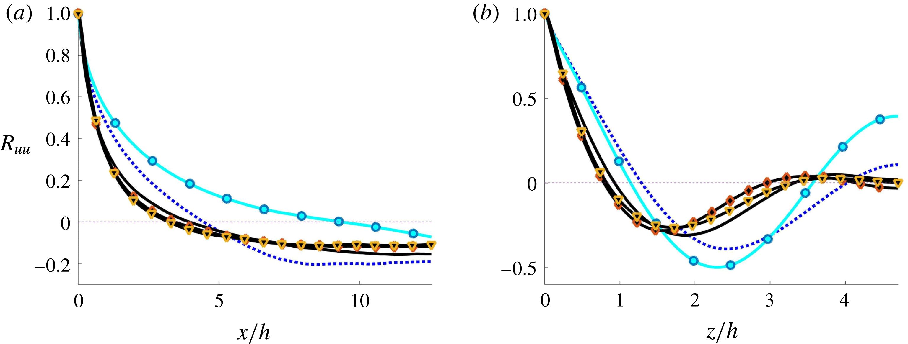
This fact is further confirmed by two-point autocorrelations, to be taken from figure 17. According to figure 17(a), the first zero in $x$ of $R_{uu}$ for the case C00 coincides with the simulation of Pirozzoli et al. (Reference Pirozzoli, Bernardini and Orlandi2011). This first zero is obtained at smaller $x$ -values, if the transpiration number is increased, indicating towards shorter structures, and, furthermore, results appear to be independent of $Re_{\unicode[STIX]{x1D70F}}$ . In the spanwise direction, figure 17(b) indicates that the situation for the two-point autocorrelation changes for large values of the transpiration velocity, and it can be seen that the second extremum, indicating towards a secondary roll, is almost zero. We may interpret that even at the largest transpiration rate, the Couette-type rolls still exist, but their strength is increasingly diminished by transpiration.

Figure 17.

Two-point autocorrelation coefficient $R_{uu}$ for $Re_{\unicode[STIX]{x1D70F}}=1000$ of velocity fluctuations at the centreline, $y/h=0$ . (a) Streamwise, (b) spanwise. Lines as in table 1.

Figure 18.

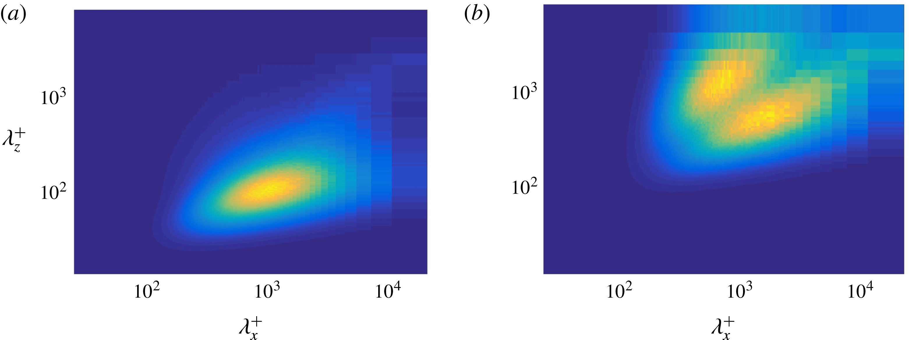
Spectral energy densities in terms of the wavelengths $\unicode[STIX]{x1D706}=2\unicode[STIX]{x03C0}/k$ for the C20 case. Spectra are normalized in wall units. (a) Suction wall, $y^{+s}\approx 15$ . (b) Blowing wall, $y^{+b}\approx 3$ .

Figure 19.

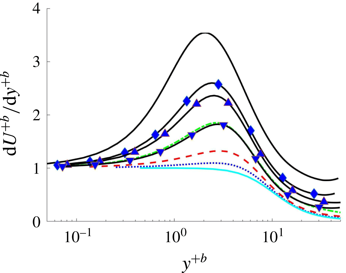
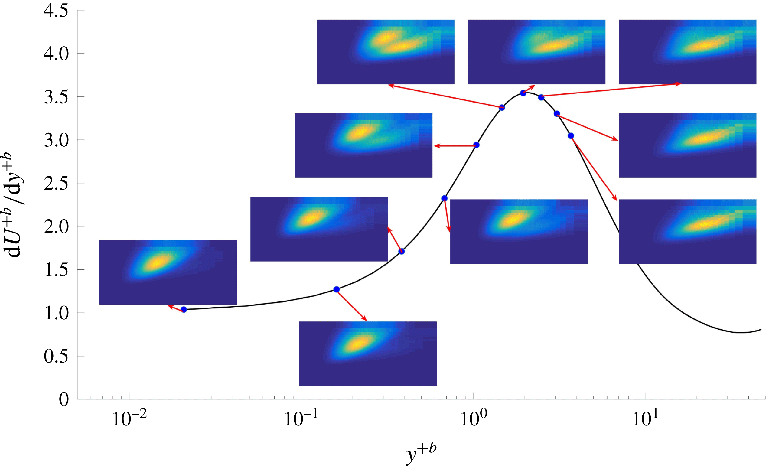
Derivative of the mean streamwise velocity with respect to $y$ scaled in blowing wall units. Lines as in table 1.

Figure 20.

Evolution of the premultiplied spectra of streamwise velocity fluctuations for case C20 in the streamwise direction. The black curve is defined as in figure 19. The points on the curve indicate the height where the different spectra were taken. After the maximum, the spectra evolve to the one expected for a classical Couette flow.

Figure 21.

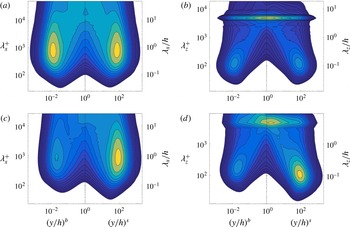
Premultiplied spectra of streamwise velocity fluctuations in the (a,c) stream- ( $k_{x}E_{uu}$ ) and (b,d) spanwise direction ( $k_{z}E_{uu}$ ). In every figure, wavelengths are given adimensionalized in both global wall units (a,c) and $h$ (b,d). The distance from the nearest wall ( $y/h$ ) is reported on the horizontal axis in logarithmic scale to emphasize the near-wall behaviour. (a,b) case C00, (c,d) case C02.

Figure 22.

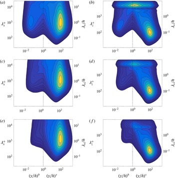
Premultiplied spectra of streamwise velocity fluctuations in the (a,c,e) stream- ( $k_{x}E_{uu}$ ) and (b,d,f) spanwise direction ( $k_{z}E_{uu}$ ). In every figure, wavelengths are given adimensionalized in both global wall units (a,c,e) and $h$ (b,d,f). The distance from the nearest wall ( $y/h$ ) is reported on the horizontal axis in logarithmic scale to emphasize the near-wall behaviour. (a,b) case C05, (c,d) case C10, (e,f) case C20.

In order to attain further structural information on the flow, we consider two-dimensional spectral energy densities $\unicode[STIX]{x1D719}=k_{x}k_{z}E(k_{x},k_{z})$ , as shown in figure 18. Two very different behaviours for the spectrum of $u$ , i.e., $\unicode[STIX]{x1D719}_{uu}$ , have been observed. The spectrum at the suction wall is presented in figure 18(a). This spectrum is similar to the one of pure Poiseuille or Couette flows (Hoyas & Jiménez Reference Hoyas and Jiménez2006; Hoyas & Jiménez Reference Hoyas and Jiménez2008; Bernardini et al. Reference Bernardini, Pirozzoli and Orlandi2014).

The situation is totally different close to the blowing wall. Figure 18(b) shows the spectrum, which we have called butterfly spectrum, at $y^{+b}\approx 3$ . Two kinds of structure, centred at two different values of $\unicode[STIX]{x1D706}$ , can be observed. They are far wider than the structures expected in this area compared to flows without transpiration. They seem to be related to an inflection point in $\overline{U}$ caused by the transpiration velocity. This inflection point appears approximately between $2<y^{+b}<3$ as soon as there is transpiration velocity, as can be seen in figure 19. The butterfly spectra disappear after the maximum of $\overline{U}$ , showing a smooth transition from wider and shorter scales than expected from the classical ones.

Concerning the situation away from the wall, the differences among the spectra of the different cases can be highlighted by representing the spectra in terms of the spanwise or streamwise wavelengths and the distance to the nearest wall. This type of representation was introduced by Hutchins & Marusic (Reference Hutchins and Marusic2007) to understand the energetic relevance of the various scales of motions at different distances from the wall. In figures 21 and 22, we see this representation for all CXX cases with the blowing side in the left columns, and the suction side in the right columns. The left columns show the premultiplied spectra in the streamwise direction, $k_{x}E_{uu}$ , and the right columns in the spanwise direction, $k_{z}E_{uu}$ . The breaking of the reflectional symmetry due to the transpiration and the flow of energy from the blowing to the suction wall can be easily seen from the latter figures. Energy in the lower half of the channel near the blowing side gradually disappears until even the peaks are lost (figure 22 e). The known maximum of the spanwise spectra in Couette flows (Pirozzoli et al. Reference Pirozzoli, Bernardini and Orlandi2014) is kept at the same position near the suction wall, approximately at $y/h\approx 0.01,\,y^{+}\approx 12$ . Energy is concentrated for all cases near $\unicode[STIX]{x1D706}_{z}^{+}\approx 110$ for the spanwise spectra in the suction half of the channel, to be taken from the right columns of figures 21 and 22. The structures appearing at the top of the spanwise spectra, at the centre of the channel at $\unicode[STIX]{x1D706}_{z}/h\approx 5$ , are the footprints of the long rolls of turbulent Couette flows without wall transpiration. Notice that as we are using logarithmic scales, there are just a few points above $\unicode[STIX]{x1D706}_{z}/h\approx 1$ , causing an anomalous shape at the top of the figures representing the spanwise spectra. From these spectra, we may conclude that although the rolls lose energy as the transpiration velocity is increased, they never fully disappear in the range of parameters that have been studied presently.