2.1. Body-forced rotating turbulence

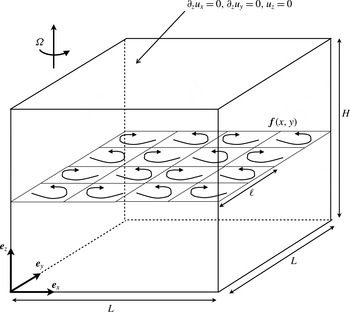
The set-up is sketched in figure 1: an incompressible fluid of kinematic viscosity ${\it\nu}$ flows inside a domain $(x,y,z)\in \mathscr{D}=[0,L]\times [0,L]\times [0,H]$ with a Cartesian frame $(\boldsymbol{e}_{x},\boldsymbol{e}_{y},\boldsymbol{e}_{z})$ . The fluid is subject to background rotation at a rate ${\it\Omega}$ around the $z$ axis, referred to as the vertical axis by convention. It is stirred by a steady divergence-free two-dimensional horizontal body force $\boldsymbol{f}(x,y)=(f_{x},f_{y},0)$ that is periodic on a scale $\ell$ , an integer fraction of $L$ . That is, $\boldsymbol{f}(x,y)=F{\bf\phi}((x/\ell ),(y/\ell ))$ , where ${\bf\phi}$ is periodic of period 1 in each dimensionless variable, has vanishing spatial mean and root-mean-square magnitude $1$ . We refer to $F$ as the amplitude and ${\bf\phi}$ as the shape of the force. We consider periodic boundary conditions in the horizontal directions and stress-free boundary conditions in the vertical (although the proofs of the present study easily carry over to a 3D periodic domain). The velocity field $\boldsymbol{u}(x,y,z,t)$ follows the rotating Navier–Stokes equation,

(2.1) $$\begin{eqnarray}\partial _{t}\boldsymbol{u}+(\boldsymbol{u}\boldsymbol{\cdot }\boldsymbol{{\rm\nabla}})\boldsymbol{u}+2{\it\Omega}\boldsymbol{e}_{z}\times \boldsymbol{u}=-\boldsymbol{{\rm\nabla}}p+{\it\nu}{\rm\Delta}\boldsymbol{u}+\boldsymbol{f},\end{eqnarray}$$

together with the following boundary conditions at the top and bottom boundaries:

(2.2a−c ) $$\begin{eqnarray}\partial _{z}u_{x}=0,\quad \partial _{z}u_{y}=0,\quad u_{z}=0,\quad \text{at }z=0\text{ and }z=H.\end{eqnarray}$$

We consider the solutions of (2.1) that have vanishing total momentum initially, and therefore at any subsequent time: the spatial average of the velocity field $\boldsymbol{u}$ is zero at all time. From (2.1) we define the Reynolds number and the Rossby number based on the root-mean-square velocity $U$ of the flow, where the mean is performed over space and time:

(2.3a,b ) $$\begin{eqnarray}Re=\frac{U\ell }{{\it\nu}},\quad Ro=\frac{U}{\ell {\it\Omega}}.\end{eqnarray}$$

We stress the fact that these dimensionless numbers combine the root-mean-square velocity $U$ of the solution with the forcing scale $\ell$ , instead of the typical scale of the velocity field (the integral scale). While the integral scale is probably close to $\ell$ for non-rotating 3D turbulence, it may increase very greatly and even reach the domain size $L$ for strong rotation, because of two-dimensionalization and enhanced inverse energy transfers. Nevertheless, the Reynolds and Rossby numbers defined in (2.3) are familiar to the theory of rotating turbulence, as well as to experimentalists: single-point velocity measurements usually lead to a good estimate of the root-mean-square velocity and allow one to estimate $Re$ and $Ro$ . Without loss of rigour, we will therefore present some results in terms of $Re$ and $Ro$ defined in (2.3).

Figure 1.

Flow of a Newtonian fluid in a frame rotating at angular velocity ${\it\Omega}$ around the vertical $z$ axis. It is driven by a horizontal body force $\boldsymbol{f}$ that is independent of the vertical. We assume periodic boundary conditions in the horizontal and stress-free boundaries at $z=0$ and $z=H$ .

We also introduce dimensionless numbers based on the strength $F$ of the forcing. The Grashof number and the forcing Rossby number are

(2.4a,b ) $$\begin{eqnarray}Gr=\frac{F\ell ^{3}}{{\it\nu}^{2}},\quad Ro^{(f)}=\frac{\sqrt{F}}{\sqrt{\ell }{\it\Omega}}.\end{eqnarray}$$

In contrast with $Re$ and $Ro$ , $Gr$ and $Ro^{(f)}$ are control parameters: they do not require knowledge of the solution to be evaluated. For instance, $Gr$ and $Ro^{(f)}$ can be specified at the outset of a numerical simulation. In the following we present both results expressed in terms of $Re$ and $Ro$ , which are useful for qualitative comparison with boundary-driven experiments, and results expressed with $Gr$ and $Ro^{(f)}$ , which are useful for comparison with body-forced numerical simulations or experiments.

In the following we use many inequalities. To alleviate the algebra somewhat, we make extensive use of the notation ${\lesssim}$ , where $a\lesssim b$ means that there is a dimensionless constant $c>0$ such that $a\leqslant cb$ , where the constant $c$ is independent of the parameters of the problem: ${\it\nu}$ , $F$ , $U$ , $\ell$ , $L$ , $H$ , etc. This constant can depend only on the precise choice of the dimensionless shape function ${\bf\phi}$ of the forcing. In the following, we denote as $c$ any such positive $\mathit{O}(1)$ constant, and we sometimes use the same symbol $c$ to denote different constants in successive lines of algebra. Numbered constants $c_{i}$ ( $\tilde{c}_{i}$ in the appendix) keep the same value between different lines of algebra.

Finally, we consider only domains that are cubic or shallower than a cube, $H\leqslant L$ , and because we focus on the large-Reynolds-number behaviour of the system, we restrict attention to $Re\geqslant 2$ and $Gr\geqslant 2$ .

2.2. Two-dimensional solutions

Equation (2.1) with the boundary conditions (2.2) admits vertically invariant 2D solutions $\boldsymbol{u}(x,y,z,t)=\boldsymbol{V}(x,y,t)$ , where $\boldsymbol{V}$ satisfies the two-dimensional Navier–Stokes equation,

(2.5) $$\begin{eqnarray}\partial _{t}\boldsymbol{V}+(\boldsymbol{V}\boldsymbol{\cdot }\boldsymbol{{\rm\nabla}})\boldsymbol{V}=-\boldsymbol{{\rm\nabla}}p+{\it\nu}{\rm\Delta}\boldsymbol{V}+\boldsymbol{f}.\end{eqnarray}$$

It should be noted that, in the 2D Navier–Stokes equation, the Coriolis force is a gradient that can be absorbed into the pressure term: ${\it\Omega}$ disappears from the equation (and we keep using $p$ to denote the modified pressure). Here, $\boldsymbol{V}(x,y,t)$ is a horizontal velocity field, with vanishing vertical component (for periodic boundary conditions in the vertical, the vertical component of $\boldsymbol{V}$ satisfies a sourceless advection–diffusion equation and therefore vanishes in the long-time limit).

Rigorous bounds on the time-averaged enstrophy and enstrophy dissipation rate can be computed for solutions of the 2D Navier–Stokes equation (2.5). The derivation of these bounds is recalled in appendix A. In terms of the forcing amplitude $F$ , and denoting as ${\it\omega}$ the vertical vorticity of the 2D flow $\boldsymbol{V}$ , we obtain

(2.6) $$\begin{eqnarray}\displaystyle & \displaystyle \langle \Vert {\it\omega}\Vert _{2}^{2}\rangle \lesssim \frac{F^{2}\ell ^{2}L^{2}H}{{\it\nu}^{2}}, & \displaystyle\end{eqnarray}$$

(2.7) $$\begin{eqnarray}\displaystyle & \displaystyle \langle \Vert \boldsymbol{{\rm\nabla}}{\it\omega}\Vert _{2}^{2}\rangle \lesssim \frac{F^{2}L^{2}H}{{\it\nu}^{2}}, & \displaystyle\end{eqnarray}$$

$\langle \ldots \rangle$

$\Vert \ldots \Vert _{2}$

$L_{2}$

(2.8) $$\begin{eqnarray}\displaystyle \Vert \boldsymbol{h}\Vert _{2}^{2}=\int _{\mathscr{D}}|\boldsymbol{h}|^{2}\,\text{d}^{3}\boldsymbol{x}. & & \displaystyle\end{eqnarray}$$

Alternate bounds were obtained by Alexakis & Doering (Reference Alexakis and Doering2006) in terms of the root-mean-square velocity $U$ . Using our notations, their equations (23) and (19) translate into

(2.9) $$\begin{eqnarray}\displaystyle \langle \Vert {\it\omega}\Vert _{2}^{2}\rangle \lesssim \frac{HL^{2}U^{2}}{\ell ^{2}}\sqrt{Re}, & & \displaystyle\end{eqnarray}$$

(2.10) $$\begin{eqnarray}\displaystyle \langle \Vert \boldsymbol{{\rm\nabla}}{\it\omega}\Vert _{2}^{2}\rangle \lesssim \frac{HL^{2}U^{2}}{\ell ^{4}}Re, & & \displaystyle\end{eqnarray}$$

$Re\geqslant 2$

These bounds for 2D flows can be further reduced if the forcing contains a single wavenumber in Fourier space, i.e. if it is such that $\boldsymbol{f}$ is an eigenmode of the Laplacian operator (see Constantin, Foias & Manley (Reference Constantin, Foias and Manley1994) for a description of 2D turbulence driven by such forcing). These forcings are sometimes called ‘single-mode’ or Kolmogorov forcings. For such forcings the improved bounds on the enstrophy and enstrophy dissipation rate are

(2.11) $$\begin{eqnarray}\displaystyle \langle \Vert {\it\omega}\Vert _{2}^{2}\rangle \lesssim \frac{HL^{2}U^{2}}{\ell ^{2}}, & & \displaystyle\end{eqnarray}$$

(2.12) $$\begin{eqnarray}\displaystyle \langle \Vert \boldsymbol{{\rm\nabla}}{\it\omega}\Vert _{2}^{2}\rangle \lesssim \frac{HL^{2}U^{2}}{\ell ^{4}}. & & \displaystyle\end{eqnarray}$$

3.1. Large versus small horizontal scales of the perturbation

From the spatial Fourier transform (3.2) of $\boldsymbol{v}$ , we define a cutoff $\mathscr{K}$ for the wavenumber $k=|\boldsymbol{k}|$ , and we write $\boldsymbol{v}=\boldsymbol{v}_{{<}}+\boldsymbol{v}_{{>}}$ , where $\boldsymbol{v}_{{<}}$ contains all of the Fourier modes with $k\leqslant \mathscr{K}$ and $\boldsymbol{v}_{{>}}$ contains all of the Fourier modes with $k>\mathscr{K}$ . Equation (3.4) becomes

(3.5) $$\begin{eqnarray}\displaystyle \frac{1}{2}\text{d}_{t}(\ln \Vert \boldsymbol{v}\Vert _{2}^{2}) & = & \displaystyle \frac{1}{\Vert \boldsymbol{v}\Vert _{2}^{2}}\left[-\int _{\mathscr{D}} [\boldsymbol{v}_{{<}}\boldsymbol{\cdot }(\boldsymbol{{\rm\nabla}}\boldsymbol{V})\boldsymbol{\cdot }\boldsymbol{v}_{{<}}+\boldsymbol{v}_{{<}}\boldsymbol{\cdot }(\boldsymbol{{\rm\nabla}}\boldsymbol{V})\boldsymbol{\cdot }\boldsymbol{v}_{{>}}+\boldsymbol{v}_{{>}}\boldsymbol{\cdot }(\boldsymbol{{\rm\nabla}}\boldsymbol{V})\boldsymbol{\cdot }\boldsymbol{v}_{{<}}\right.\nonumber\\ \displaystyle & & \displaystyle +\,\left.\vphantom{\int _{\mathscr{D}}}\boldsymbol{v}_{{>}}\boldsymbol{\cdot }(\boldsymbol{{\rm\nabla}}\boldsymbol{V})\boldsymbol{\cdot }\boldsymbol{v}_{{>}} ]\,\text{d}^{3}\boldsymbol{x}-{\it\nu}\Vert \boldsymbol{{\rm\nabla}}\boldsymbol{v}\Vert _{2}^{2}\right].\end{eqnarray}$$

We now bound all of the terms on the right-hand side that involve $\boldsymbol{v}_{{>}}$ . Using successively Hölder’s, the Cauchy–Schwarz and Young’s inequalities together with an optimization,

(3.6) $$\begin{eqnarray}\displaystyle & & \displaystyle \left|\int _{\mathscr{D}}[\boldsymbol{v}_{{<}}\boldsymbol{\cdot }(\boldsymbol{{\rm\nabla}}\boldsymbol{V})\boldsymbol{\cdot }\boldsymbol{v}_{{>}}+\boldsymbol{v}_{{>}}\boldsymbol{\cdot }(\boldsymbol{{\rm\nabla}}\boldsymbol{V})\boldsymbol{\cdot }\boldsymbol{v}_{{<}}+\boldsymbol{v}_{{>}}\boldsymbol{\cdot }(\boldsymbol{{\rm\nabla}}\boldsymbol{V})\boldsymbol{\cdot }\boldsymbol{v}_{{>}}]\,\text{d}^{3}\boldsymbol{x}\right|\nonumber\\ \displaystyle & & \displaystyle \quad \leqslant \Vert \boldsymbol{{\rm\nabla}}\boldsymbol{V}\Vert _{\infty }[2\Vert \boldsymbol{v}_{{<}}\Vert _{2}\Vert \boldsymbol{v}_{{>}}\Vert _{2}+\Vert \boldsymbol{v}_{{>}}\Vert _{2}^{2}]\nonumber\\ \displaystyle & & \displaystyle \quad \leqslant \frac{{\it\nu}\mathscr{K}^{2}}{4}\Vert \boldsymbol{v}_{{>}}\Vert _{2}^{2}+\frac{4}{{\it\nu}\mathscr{K}^{2}}\Vert \boldsymbol{{\rm\nabla}}\boldsymbol{V}\Vert _{\infty }^{2}\Vert \boldsymbol{v}_{{<}}\Vert _{2}^{2}+\frac{{\it\nu}\mathscr{K}^{2}}{4}\Vert \boldsymbol{v}_{{>}}\Vert _{2}^{2}+\frac{1}{{\it\nu}\mathscr{K}^{2}}\Vert \boldsymbol{{\rm\nabla}}\boldsymbol{V}\Vert _{\infty }^{2}\Vert \boldsymbol{v}_{{>}}\Vert _{2}^{2}\nonumber\\ \displaystyle & & \displaystyle \quad \leqslant \frac{{\it\nu}\mathscr{K}^{2}}{2}\Vert \boldsymbol{v}_{{>}}\Vert _{2}^{2}+\frac{4}{{\it\nu}\mathscr{K}^{2}}\Vert \boldsymbol{{\rm\nabla}}\boldsymbol{V}\Vert _{\infty }^{2}\Vert \boldsymbol{v}\Vert _{2}^{2},\end{eqnarray}$$

where $\Vert \ldots \Vert _{\infty }$ denotes the standard $L_{\infty }$ norm in space. From Poincaré’s inequality, $\Vert \boldsymbol{{\rm\nabla}}\boldsymbol{v}_{{>}}\Vert _{2}^{2}\geqslant \mathscr{K}^{2}\Vert \boldsymbol{v}_{{>}}\Vert _{2}^{2}$ and $\Vert \boldsymbol{{\rm\nabla}}\boldsymbol{v}\Vert _{2}^{2}\geqslant ({\rm\pi}^{2}/H^{2})\Vert \boldsymbol{v}\Vert _{2}^{2}$ , hence

(3.7) $$\begin{eqnarray}\displaystyle -{\it\nu}\Vert \boldsymbol{{\rm\nabla}}\boldsymbol{v}\Vert _{2}^{2}\leqslant -\frac{{\it\nu}}{4}\Vert \boldsymbol{{\rm\nabla}}\boldsymbol{v}\Vert _{2}^{2}-\frac{{\it\nu}\mathscr{K}^{2}}{2}\Vert \boldsymbol{v}_{{>}}\Vert _{2}^{2}-\frac{{\it\nu}{\rm\pi}^{2}}{4H^{2}}\Vert \boldsymbol{v}\Vert _{2}^{2}. & & \displaystyle\end{eqnarray}$$

Inserting inequalities (3.6) and (3.7) in (3.5) results in

(3.8) $$\begin{eqnarray}\displaystyle \frac{1}{2}\text{d}_{t}(\ln \Vert \boldsymbol{v}\Vert _{2}^{2})\leqslant \frac{1}{\Vert \boldsymbol{v}\Vert _{2}^{2}}\left[-\int _{\mathscr{D}}\boldsymbol{v}_{{<}}\boldsymbol{\cdot }(\boldsymbol{{\rm\nabla}}\boldsymbol{V})\boldsymbol{\cdot }\boldsymbol{v}_{{<}}\,\text{d}^{3}\boldsymbol{x}-\frac{{\it\nu}}{4}\Vert \boldsymbol{{\rm\nabla}}\boldsymbol{v}\Vert _{2}^{2}\right]+{\it\lambda}_{1}(t), & & \displaystyle\end{eqnarray}$$

where ${\it\lambda}_{1}(t)=(4/{\it\nu}\mathscr{K}^{2})\Vert \boldsymbol{{\rm\nabla}}\boldsymbol{V}\Vert _{\infty }^{2}-({\it\nu}{\rm\pi}^{2}/4H^{2})$ . It should be noticed that the triple velocity product in (3.8) does not involve $\boldsymbol{v}_{{>}}$ anymore. In the following we choose the value

(3.9) $$\begin{eqnarray}\displaystyle \mathscr{K}=\frac{\sqrt{32}H}{{\rm\pi}{\it\nu}}\sqrt{\langle \Vert \boldsymbol{{\rm\nabla}}\boldsymbol{ V}\Vert _{\infty }^{2}\rangle }, & & \displaystyle\end{eqnarray}$$

which leads to the following time average of ${\it\lambda}_{1}(t)$ :

(3.10) $$\begin{eqnarray}\displaystyle \langle {\it\lambda}_{1}\rangle =-\frac{{\it\nu}{\rm\pi}^{2}}{8H^{2}}, & & \displaystyle\end{eqnarray}$$

which is sufficient control over small horizontal scales $\boldsymbol{v}_{{>}}$ of the perturbation. The quantity $\langle \Vert \boldsymbol{{\rm\nabla}}\boldsymbol{V}\Vert _{\infty }^{2}\rangle$ is bounded from above in appendix A, which provides an upper bound on $\mathscr{K}$ ,

(3.11) $$\begin{eqnarray}\displaystyle \mathscr{K}\lesssim \frac{\sqrt{H}}{{\it\nu}}\sqrt{\langle \Vert \boldsymbol{{\rm\nabla}}{\it\omega}\Vert _{2}^{2}\rangle }\ln ^{1/2}\left(Gr\frac{L}{\ell }\right), & & \displaystyle\end{eqnarray}$$

where the right-hand side involves the time-averaged enstrophy dissipation rate of the 2D base flow, which can be bounded in terms of its root-mean-square velocity $U$ using (2.10) or (2.12), or in terms of the forcing strength $F$ using (2.7).

6.1. Combining the bounds on the four terms

Inserting (5.2) into (5.1), with $K\geqslant {\rm\pi}/H\geqslant 1/H$ , leads to the following inequality:

(6.1) $$\begin{eqnarray}\displaystyle \frac{1}{T}\ln \frac{\Vert \boldsymbol{v}\Vert _{2}(t=T)}{\Vert \boldsymbol{v}\Vert _{2}(t=0)} & {\leqslant} & \displaystyle \frac{L^{2}H^{2}}{2{\it\Omega}}(|\mathscr{T}_{1}|+|\mathscr{T}_{2}|+|\mathscr{T}_{3}|+|\mathscr{T}_{4}|)\nonumber\\ \displaystyle & & \displaystyle -\,\frac{{\it\nu}}{4T}\int _{t=0}^{t=T}\frac{\Vert \boldsymbol{{\rm\nabla}}\boldsymbol{v}\Vert _{2}^{2}}{\Vert \boldsymbol{v}\Vert _{2}^{2}}\,\text{d}t+\frac{1}{T}\int _{t=0}^{t=T}{\it\lambda}_{1}(t)\,\text{d}t.\end{eqnarray}$$

Our goal is to show that the right-hand side of this inequality is negative in the limit $T\rightarrow \infty$ , provided that ${\it\Omega}$ is large enough. We substitute the bounds (5.21) and (5.24) on $|\mathscr{T}_{2}|$ and $|\mathscr{T}_{3}|$ , which indicate that there are two positive dimensionless constants $c_{2}$ and $c_{3}$ such that

(6.2) $$\begin{eqnarray}\displaystyle \frac{1}{T}\ln \frac{\Vert \boldsymbol{v}\Vert _{2}(t=T)}{\Vert \boldsymbol{v}\Vert _{2}(t=0)} & {\leqslant} & \displaystyle \frac{1}{T}\int _{t=0}^{t=T}{\it\lambda}_{1}(t)\,\text{d}t+\frac{L^{2}H^{2}}{2{\it\Omega}}(|\mathscr{T}_{1}|+|\mathscr{T}_{4}|)\nonumber\\ \displaystyle & & \displaystyle +\,c_{3}\frac{H^{3/2}\langle \Vert \boldsymbol{{\rm\nabla}}{\it\omega}\Vert _{2}^{2}\rangle }{{\it\Omega}{\it\nu}^{2}}\ln ^{3/2}\left(Gr\frac{L}{\ell }\right)\frac{1}{T}\int _{t=0}^{t=T}\Vert {\it\omega}\Vert _{2}\Vert \boldsymbol{{\rm\nabla}}\boldsymbol{V}\Vert _{\infty }\,\text{d}t\nonumber\\ \displaystyle & & \displaystyle +\,\left[\frac{L^{2}H^{2}\langle \Vert \boldsymbol{{\rm\nabla}}{\it\omega}\Vert _{2}^{2}\rangle }{\ell ^{3}{\it\Omega}}Gr\ln ^{3/2}\left(Gr\frac{L}{\ell }\right)\left(c_{3}+c_{2}Gr\frac{L^{2}(H+\ell )}{\ell ^{3}}\right)-\frac{{\it\nu}}{4}\right]\nonumber\\ \displaystyle & & \displaystyle \times \,\frac{1}{T}\int _{t=0}^{t=T}\frac{\Vert \boldsymbol{{\rm\nabla}}\boldsymbol{v}\Vert _{2}^{2}}{\Vert \boldsymbol{v}\Vert _{2}^{2}}\,\text{d}t.\end{eqnarray}$$

Because we focus on $Gr\geqslant 2$ , we have $c_{3}+c_{2}Gr((L^{2}(H+\ell ))/\ell ^{3})\leqslant c_{4}Gr$   $((L^{2}(H+\ell ))/\ell ^{3})$ , with $c_{4}=\max (c_{2};c_{3})$ . Hence, a sufficient condition for the square bracket in (6.2) to be negative is

(6.3) $$\begin{eqnarray}\displaystyle {\it\Omega}\geqslant {\it\Omega}_{1}=4c_{4}\frac{L^{4}H^{2}(H+\ell )}{\ell ^{6}}\frac{\langle \Vert \boldsymbol{{\rm\nabla}}{\it\omega}\Vert _{2}^{2}\rangle }{{\it\nu}}Gr^{2}\ln ^{3/2}\left(Gr\frac{L}{\ell }\right). & & \displaystyle\end{eqnarray}$$

When this condition is satisfied, one can drop the last term in (6.2). Then, upon taking the limit $T\rightarrow \infty$ , using the Cauchy–Schwarz inequality for the middle line together with $\langle {\it\lambda}_{1}(t)\rangle =-{\it\nu}{\rm\pi}^{2}/(8H^{2})$ , $\lim _{T\rightarrow \infty }|\mathscr{T}_{4}|=0$ , the bound (5.12) on $\lim _{T\rightarrow \infty }|\mathscr{T}_{1}|$ and (A 33),

(6.4) $$\begin{eqnarray}\displaystyle & & \displaystyle \lim _{T\rightarrow \infty }\frac{1}{T}\ln \frac{\Vert \boldsymbol{v}\Vert _{2}(t=T)}{\Vert \boldsymbol{v}\Vert _{2}(t=0)}\nonumber\\ \displaystyle & & \displaystyle \quad \leqslant \langle {\it\lambda}_{1}(t)\rangle +\frac{L^{2}H^{2}}{2{\it\Omega}}\left(\lim _{T\rightarrow \infty }|\mathscr{T}_{1}|+\lim _{T\rightarrow \infty }|\mathscr{T}_{4}|\right)\nonumber\\ \displaystyle & & \displaystyle \qquad +\,c_{3}\frac{H^{3/2}\langle \Vert \boldsymbol{{\rm\nabla}}{\it\omega}\Vert _{2}^{2}\rangle }{{\it\Omega}{\it\nu}^{2}}\ln ^{3/2}\left(Gr\frac{L}{\ell }\right)\sqrt{\langle \Vert {\it\omega}\Vert _{2}^{2}\rangle \langle \Vert \boldsymbol{{\rm\nabla}}\boldsymbol{ V}\Vert _{\infty }^{2}\rangle }\nonumber\\ \displaystyle & & \displaystyle \quad \leqslant -\frac{{\it\nu}{\rm\pi}^{2}}{8H^{2}}+\frac{c_{1}H^{2}}{{\it\nu}^{2}{\it\Omega}}\langle \Vert \boldsymbol{{\rm\nabla}}{\it\omega}\Vert _{2}^{2}\rangle \ln \left(Gr\frac{L}{\ell }\right)\nonumber\\ \displaystyle & & \displaystyle \qquad \times \,\left[\frac{FL^{2}}{\ell ^{2}}+\left(\frac{1}{H}\sqrt{\langle \Vert {\it\omega}\Vert _{2}^{2}\rangle \langle \Vert \boldsymbol{{\rm\nabla}}{\it\omega}\Vert _{2}^{2}\rangle }+\langle \Vert \boldsymbol{{\rm\nabla}}{\it\omega}\Vert _{2}^{2}\rangle \right)\ln \left(Gr\frac{L}{\ell }\right)\right]\nonumber\\ \displaystyle & & \displaystyle \qquad +\,c_{3}\frac{H^{3/2}\langle \Vert \boldsymbol{{\rm\nabla}}{\it\omega}\Vert _{2}^{2}\rangle }{{\it\Omega}{\it\nu}^{2}}\ln ^{3/2}\left(Gr\frac{L}{\ell }\right)\sqrt{\langle \Vert {\it\omega}\Vert _{2}^{2}\rangle \langle \Vert \boldsymbol{{\rm\nabla}}\boldsymbol{ V}\Vert _{\infty }^{2}\rangle }\nonumber\\ \displaystyle & & \displaystyle \quad \leqslant -\frac{{\it\nu}{\rm\pi}^{2}}{8H^{2}}+\frac{H^{2}}{{\it\nu}^{2}{\it\Omega}}\langle \Vert \boldsymbol{{\rm\nabla}}{\it\omega}\Vert _{2}^{2}\rangle \ln \left(Gr\frac{L}{\ell }\right)\nonumber\\ \displaystyle & & \displaystyle \qquad \times \left[c_{1}\frac{FL^{2}}{\ell ^{2}}+\left(\frac{c_{1}+c_{3}\sqrt{\tilde{c}_{2}}}{H}\sqrt{\langle \Vert {\it\omega}\Vert _{2}^{2}\rangle \langle \Vert \boldsymbol{{\rm\nabla}}{\it\omega}\Vert _{2}^{2}\rangle }+c_{1}\langle \Vert \boldsymbol{{\rm\nabla}}{\it\omega}\Vert _{2}^{2}\rangle \right)\ln \left(Gr\frac{L}{\ell }\right)\right],\qquad\end{eqnarray}$$

$c_{1}$

(6.5) $$\begin{eqnarray}\displaystyle {\it\Omega}\geqslant {\it\Omega}_{2} & = & \displaystyle c_{5}\frac{H^{4}\langle \Vert \boldsymbol{{\rm\nabla}}{\it\omega}\Vert _{2}^{2}\rangle }{{\it\nu}^{3}}\ln \left(Gr\frac{L}{\ell }\right)\nonumber\\ \displaystyle & & \displaystyle \times \left[\frac{FL^{2}}{\ell ^{2}}+\left(\frac{1}{H}\sqrt{\langle \Vert {\it\omega}\Vert _{2}^{2}\rangle \langle \Vert \boldsymbol{{\rm\nabla}}{\it\omega}\Vert _{2}^{2}\rangle }+\langle \Vert \boldsymbol{{\rm\nabla}}{\it\omega}\Vert _{2}^{2}\rangle \right)\ln \left(Gr\frac{L}{\ell }\right)\right],\end{eqnarray}$$

where $c_{5}=c_{1}+c_{3}\sqrt{\tilde{c}_{2}}$ .

To summarize, if ${\it\Omega}>{\it\Omega}_{1}$ and ${\it\Omega}>{\it\Omega}_{2}$ , where ${\it\Omega}_{1}$ and ${\it\Omega}_{2}$ are defined in (6.3) and (6.5) respectively, then

(6.6) $$\begin{eqnarray}\displaystyle \lim _{T\rightarrow \infty }\frac{1}{T}\ln \frac{\Vert \boldsymbol{v}\Vert _{2}(t=T)}{\Vert \boldsymbol{v}\Vert _{2}(t=0)}<0, & & \displaystyle\end{eqnarray}$$

and therefore $\lim _{t\rightarrow \infty }\Vert \boldsymbol{v}\Vert _{2}(t)=0$ : the 2D base flow is linearly stable to 3D perturbations.

As a matter of fact, using the bounds (2.6) and (2.7) one can prove that ${\it\Omega}_{2}\lesssim {\it\Omega}_{1}\ln ^{1/2}(Gr(L/\ell ))$ . Hence, ${\it\Omega}\geqslant c{\it\Omega}_{1}\ln ^{1/2}(Gr(L/\ell ))$ is a sufficient condition to have both ${\it\Omega}\geqslant {\it\Omega}_{1}$ and ${\it\Omega}\geqslant {\it\Omega}_{2}$ . We therefore obtain the following sufficient condition for the flow to be linearly stable to 3D perturbations:

(6.7) $$\begin{eqnarray}\displaystyle {\it\Omega}\geqslant {\it\Omega}_{3}=c_{6}\frac{\langle \Vert \boldsymbol{{\rm\nabla}}{\it\omega}\Vert _{2}^{2}\rangle }{{\it\nu}}Gr^{2}\ln ^{2}\left(Gr\frac{L}{\ell }\right)\frac{L^{4}H^{2}(H+\ell )}{\ell ^{6}}, & & \displaystyle\end{eqnarray}$$

where $c_{6}$ is a dimensionless constant.

6.2. Criteria based on the root-mean-square velocity

The sufficient condition (6.7) indicates unambiguously that the flow is linearly stable to three-dimensional perturbations above a critical value of the rotation rate ${\it\Omega}$ . However, the quantity $\langle \Vert \boldsymbol{{\rm\nabla}}{\it\omega}\Vert _{2}^{2}\rangle$ appearing in this criterion is difficult to measure or evaluate. We therefore use the bounds (2.10) and (2.12) on the time-averaged enstrophy dissipation rate, together with (A 2) and (A 10), to produce alternate sufficient conditions for two-dimensionalization that are expressed in terms of the root-mean-square velocity $U$ .

The bound (2.10) gives

(6.8) $$\begin{eqnarray}\displaystyle \frac{\ell {\it\Omega}_{3}}{U}\lesssim Re^{6}\ln ^{2}\left(Re\frac{L}{\ell }\right)\frac{L^{6}H^{3}(H+\ell )}{\ell ^{10}}, & & \displaystyle\end{eqnarray}$$

hence the two-dimensional flow is stable if the inverse Rossby number is greater than the right-hand side of this inequality, i.e. if

(6.9) $$\begin{eqnarray}\displaystyle Ro\leqslant Ro_{{<}}=c_{7}Re^{-6}\ln ^{-2}\left(Re\frac{L}{\ell }\right)\frac{\ell ^{10}}{L^{6}H^{3}(H+\ell )}, & & \displaystyle\end{eqnarray}$$

where $c_{7}$ is a dimensionless constant that depends on the shape of the forcing only.

A somewhat less stringent criterion for two-dimensionalization can be obtained when the forcing is of single-mode type. By bounding $\langle \Vert \boldsymbol{{\rm\nabla}}{\it\omega}\Vert _{2}^{2}\rangle$ in ${\it\Omega}_{3}$ using (2.12), we obtain the following sufficient condition for the decay of infinitesimal 3D perturbations:

(6.10) $$\begin{eqnarray}\displaystyle Ro\leqslant Ro_{{<}}^{(\mathit{SM})}=c_{8}Re^{-5}\ln ^{-2}\left(Re\frac{L}{\ell }\right)\frac{\ell ^{10}}{L^{6}H^{3}(H+\ell )}, & & \displaystyle\end{eqnarray}$$

where $c_{8}$ is yet another dimensionless constant that depends on the shape of the forcing only.

6.3. Criterion based on the forcing strength

We can derive an alternate sufficient criterion for two-dimensionalization in terms of the forcing strength instead of the root-mean-square velocity. Inserting the upper bound (2.7) on the time-averaged enstrophy dissipation rate into the expression for ${\it\Omega}_{3}$ leads to a criterion in terms of the Grashof and forcing Rossby numbers:

(6.11) $$\begin{eqnarray}\displaystyle Ro^{(f)}\leqslant Ro_{{<}}^{(f)}=c_{9}Gr^{-7/2}\ln ^{-2}\left(Gr\frac{L}{\ell }\right)\frac{\ell ^{10}}{L^{6}H^{3}(H+\ell )}, & & \displaystyle\end{eqnarray}$$

where $c_{9}$ is a dimensionless constant that depends on the shape of the forcing only. When (6.11) is satisfied, the global attractor of the 2D Navier–Stokes equation is stable to infinitesimal 3D perturbations.

7.1. Evolution of the three-dimensional part of the velocity field

We consider the evolution of an initially 3D velocity field under the fully nonlinear 3D rotating Navier–Stokes equation (2.1). We define the vertical average of a field $\boldsymbol{h}$ as

(7.3) $$\begin{eqnarray}\bar{\boldsymbol{h}}(x,y,t)=\frac{1}{H}\int _{z=0}^{z=H}\boldsymbol{h}(x,y,z,t)\,\text{d}z,\end{eqnarray}$$

and decompose the velocity field into

(7.4) $$\begin{eqnarray}\boldsymbol{u}=\boldsymbol{V}(x,y,t)+\boldsymbol{v}(x,y,z,t),\quad \text{with }\boldsymbol{V}=\bar{\boldsymbol{u}}\text{ and }\boldsymbol{v}=\boldsymbol{u}-\boldsymbol{V}.\end{eqnarray}$$

In the following we call $\boldsymbol{V}$ (respectively $\boldsymbol{v}$ ) the two-dimensional (respectively three-dimensional) part of the velocity field. In contrast to the previous sections, here the 3D part $\boldsymbol{v}$ of the velocity field need not be small. Our goal is to find a criterion that ensures the decay of $\boldsymbol{v}$ . The evolution equation for the two-dimensional part of the velocity field is obtained by vertically averaging equation (2.1),

(7.5) $$\begin{eqnarray}\partial _{t}\boldsymbol{V}+(\boldsymbol{V}\boldsymbol{\cdot }\boldsymbol{{\rm\nabla}})\boldsymbol{V}+\overline{(\boldsymbol{v}\boldsymbol{\cdot }\boldsymbol{{\rm\nabla}})\boldsymbol{v}}=-\boldsymbol{{\rm\nabla}}P+{\it\nu}{\rm\Delta}\boldsymbol{V}+\boldsymbol{f}(x,y),\end{eqnarray}$$

where $P$ includes the vertically averaged pressure and the vertically averaged Coriolis force, which is a gradient.

By subtracting this equation from the rotating Navier–Stokes equation, we obtain the evolution equation for the three-dimensional part of the flow:

(7.6) $$\begin{eqnarray}\partial _{t}\boldsymbol{v}+(\boldsymbol{V}\boldsymbol{\cdot }\boldsymbol{{\rm\nabla}})\boldsymbol{v}+(\boldsymbol{v}\boldsymbol{\cdot }\boldsymbol{{\rm\nabla}})\boldsymbol{V}+(\boldsymbol{v}\boldsymbol{\cdot }\boldsymbol{{\rm\nabla}})\boldsymbol{v}-\overline{(\boldsymbol{v}\boldsymbol{\cdot }\boldsymbol{{\rm\nabla}})\boldsymbol{v}}+2{\it\Omega}\boldsymbol{e}_{z}\times \boldsymbol{v}=-\boldsymbol{{\rm\nabla}}(\,p-P)+{\it\nu}{\rm\Delta}\boldsymbol{v}.\end{eqnarray}$$

Incompressibility imposes $\boldsymbol{{\rm\nabla}}\boldsymbol{\cdot }\boldsymbol{V}=0$ and $\boldsymbol{{\rm\nabla}}\boldsymbol{\cdot }\boldsymbol{v}=0$ .

7.2. Control over the small scales of the 3D part of the velocity field

One can obtain the same equation as (3.4) for the evolution of the kinetic energy of the 3D part of the velocity field, where $\boldsymbol{V}$ and $\boldsymbol{v}$ are now solutions of (7.5) and (7.6). Like in § 3.1, we introduce a cutoff wavenumber $\mathscr{K}_{\mathit{abs}}$ and decompose the 3D part of the velocity field into $\boldsymbol{v}=\boldsymbol{v}_{{<}}+\boldsymbol{v}_{{>}}$ , distinguishing between wavenumbers that are lower or greater than $\mathscr{K}_{\mathit{abs}}$ . We then repeat the steps (3.5)–(3.8), and obtain

(7.7) $$\begin{eqnarray}\displaystyle \frac{1}{2}\,\text{d}_{t}(\ln \Vert \boldsymbol{v}\Vert _{2}^{2})\leqslant \frac{1}{\Vert \boldsymbol{v}\Vert _{2}^{2}}\left[-\!\int _{\mathscr{D}}\boldsymbol{v}_{{<}}\boldsymbol{\cdot }(\boldsymbol{{\rm\nabla}}\boldsymbol{V})\boldsymbol{\cdot }\boldsymbol{v}_{{<}}\,\text{d}^{3}\boldsymbol{x}-\frac{{\it\nu}}{4}\Vert \boldsymbol{{\rm\nabla}}\boldsymbol{v}\Vert _{2}^{2}\right]\!+\frac{4}{{\it\nu}{\mathscr{K}_{\mathit{abs}}}^{2}}\Vert \boldsymbol{{\rm\nabla}}\boldsymbol{V}\Vert _{\infty }^{2}-\frac{{\it\nu}{\rm\pi}^{2}}{4H^{2}}. & & \displaystyle \nonumber\\ \displaystyle & & \displaystyle\end{eqnarray}$$

We choose the following value of the cutoff wavenumber:

(7.8) $$\begin{eqnarray}\displaystyle \mathscr{K}_{\mathit{abs}}=\frac{4H}{{\it\nu}{\rm\pi}}\sup _{t>T_{0}}\Vert \boldsymbol{{\rm\nabla}}\boldsymbol{V}\Vert _{\infty }, & & \displaystyle\end{eqnarray}$$

which we know to be a finite quantity thanks to (7.2). This ensures that the sum of the last two terms in (7.7) is negative and can be discarded (again for $t>T_{0}$ ), which leads to

(7.9) $$\begin{eqnarray}\displaystyle \frac{1}{2}\,\text{d}_{t}(\ln \Vert \boldsymbol{v}\Vert _{2}^{2})\leqslant \frac{1}{\Vert \boldsymbol{v}\Vert _{2}^{2}}\left[-\int _{\mathscr{D}}\boldsymbol{v}_{{<}}\boldsymbol{\cdot }(\boldsymbol{{\rm\nabla}}\boldsymbol{V})\boldsymbol{\cdot }\boldsymbol{v}_{{<}}\,\text{d}^{3}\boldsymbol{x}-\frac{{\it\nu}}{4}\Vert \boldsymbol{{\rm\nabla}}\boldsymbol{v}\Vert _{2}^{2}\right]. & & \displaystyle\end{eqnarray}$$

From (7.2), the cutoff wavenumber (7.8) is bounded by an ${\it\Omega}$ -independent and time-independent quantity:

(7.10) $$\begin{eqnarray}\displaystyle \mathscr{K}_{\mathit{abs}}\leqslant \frac{4H}{{\it\nu}{\rm\pi}}\sup _{t>T_{0}}\Vert \boldsymbol{{\rm\nabla}}\boldsymbol{u}\Vert _{\infty }\leqslant C. & & \displaystyle\end{eqnarray}$$

7.3. Control over the large scales of the 3D part of the velocity field

We decompose $\boldsymbol{v}$ and $\boldsymbol{V}$ on the basis of helical modes as in (4.1) and (4.4). Inserting these decompositions into the evolution equation (7.6) and projecting onto each helical mode leads to the evolution equation for the helical amplitudes of $\boldsymbol{v}$ :

(7.11) $$\begin{eqnarray}\displaystyle \partial _{t}b_{s_{\boldsymbol{k}}}=-{\it\nu}k^{2}b_{s_{\boldsymbol{k}}}+\mathop{\sum }_{\substack{ \boldsymbol{p}+\boldsymbol{q}+\boldsymbol{k}=0 \\ s_{\boldsymbol{p}};s_{\boldsymbol{q}}}}C_{\boldsymbol{k}\boldsymbol{p}\boldsymbol{q}}^{s_{\boldsymbol{k}}s_{\boldsymbol{p}}s_{\boldsymbol{q}}}\,\left[b_{s_{\boldsymbol{p}}}^{\ast }B_{s_{\boldsymbol{q}}}^{\ast }\text{e}^{-\text{i}({\it\sigma}_{s_{\boldsymbol{p}}}+{\it\sigma}_{s_{\boldsymbol{k}}}\!)t}+\frac{1}{2}b_{s_{\boldsymbol{p}}}^{\ast }b_{s_{\boldsymbol{q}}}^{\ast }\text{e}^{-\text{i}({\it\sigma}_{s_{\boldsymbol{p}}}+{\it\sigma}_{s_{\boldsymbol{k}}}+{\it\sigma}_{s_{\boldsymbol{q}}}\!)t}\right], & & \displaystyle\end{eqnarray}$$

where $C_{\boldsymbol{k}\boldsymbol{p}\boldsymbol{q}}^{s_{\boldsymbol{k}}s_{\boldsymbol{p}}s_{\boldsymbol{q}}}$ is still given by (4.8). Using the vorticity equation for the 2D part of the flow, we obtain the following evolution equation for the helical amplitudes of $\boldsymbol{V}$ :

(7.12) $$\begin{eqnarray}\displaystyle \partial _{t}B_{s_{\boldsymbol{k}}}=\frac{-s_{\boldsymbol{k}}}{\sqrt{2}k}[-\text{i}\boldsymbol{k}\boldsymbol{\cdot }\{{\it\omega}\boldsymbol{V}\}_{\boldsymbol{k}}+(\text{i}\boldsymbol{k}\times \{\overline{\boldsymbol{v}\times (\boldsymbol{{\rm\nabla}}\times \boldsymbol{v})}\}_{\boldsymbol{k}})\boldsymbol{\cdot }\boldsymbol{e}_{z}-{\it\nu}k^{2}{\it\omega}_{\boldsymbol{k}}+(\text{i}\boldsymbol{k}\times \boldsymbol{f}_{\boldsymbol{k}})\boldsymbol{\cdot }\boldsymbol{e}_{z}],\quad & & \displaystyle\end{eqnarray}$$

where $\boldsymbol{f}_{\boldsymbol{k}}$ and ${\it\omega}_{\boldsymbol{k}}$ are the Fourier amplitudes of $\boldsymbol{f}$ and ${\it\omega}$ , using Fourier series similar to (3.2) and (4.3). Similarly, $\{\ldots \!\,\}_{\boldsymbol{k}}$ denotes the Fourier amplitude of its argument on the wavevector $\boldsymbol{k}$ .

In contrast to the proof of linear two-dimensionalization, here the 3D part of the velocity field contains many Fourier modes in $z$ , the evolution of which is coupled. On writing the vertical component of $\boldsymbol{k}$ as $k_{z}=n{\rm\pi}/H$ , with $n\in \mathbb{Z}_{\neq 0}=\mathbb{Z}\setminus \{0\}$ , the triple velocity product becomes

(7.13) $$\begin{eqnarray}\displaystyle & & \displaystyle \int _{\mathscr{D}}\boldsymbol{v}_{{<}}\boldsymbol{\cdot }(\boldsymbol{{\rm\nabla}}\boldsymbol{V})\boldsymbol{\cdot }\boldsymbol{v}_{{<}}\,\text{d}^{3}\boldsymbol{x}\nonumber\\ \displaystyle & & \displaystyle \quad =-L^{2}H\mathop{\sum }_{n\in \mathbb{Z}_{\neq 0}}\mathop{\sum }_{\substack{ \boldsymbol{p}+\boldsymbol{q}+\boldsymbol{k}=0 \\ k_{z}=n{\rm\pi}/H;k\leqslant \mathscr{K}_{\mathit{abs}};p\leqslant \mathscr{K}_{\mathit{abs}} \\ s_{\boldsymbol{p}};s_{\boldsymbol{q}};s_{\boldsymbol{k}}}}B_{s_{\boldsymbol{q}}}b_{s_{\boldsymbol{k}}}b_{s_{\boldsymbol{p}}}\text{e}^{\text{i}({\it\sigma}_{s_{\boldsymbol{k}}}+{\it\sigma}_{s_{\boldsymbol{p}}})t}s_{\boldsymbol{ k}}s_{\boldsymbol{p}}kp\frac{{\it\sigma}_{s_{\boldsymbol{k}}}+{\it\sigma}_{s_{\boldsymbol{p}}}}{2{\it\Omega}k_{z}}g_{\boldsymbol{q}\boldsymbol{k}\boldsymbol{p}}^{\ast s_{\boldsymbol{q}}s_{\boldsymbol{k}}s_{\boldsymbol{p}}}\nonumber\\ \displaystyle & & \displaystyle \quad =-\frac{L^{2}H^{2}}{{\rm\pi}}\mathop{\sum }_{n\in \mathbb{Z}_{\neq 0}}\frac{1}{n}\mathop{\sum }_{\substack{ \boldsymbol{p}+\boldsymbol{q}+\boldsymbol{k}=0 \\ k_{z}=n{\rm\pi}/H;k\leqslant \mathscr{K}_{\mathit{abs}};p\leqslant \mathscr{K}_{\mathit{abs}} \\ s_{\boldsymbol{p}};s_{\boldsymbol{q}};s_{\boldsymbol{k}}}}B_{s_{\boldsymbol{q}}}b_{s_{\boldsymbol{k}}}b_{s_{\boldsymbol{p}}}\text{e}^{\text{i}({\it\sigma}_{s_{\boldsymbol{k}}}+{\it\sigma}_{s_{\boldsymbol{p}}})t}s_{\boldsymbol{ k}}s_{\boldsymbol{p}}kp\frac{{\it\sigma}_{s_{\boldsymbol{k}}}+{\it\sigma}_{s_{\boldsymbol{p}}}}{2{\it\Omega}}g_{\boldsymbol{q}\boldsymbol{k}\boldsymbol{p}}^{\ast s_{\boldsymbol{q}}s_{\boldsymbol{k}}s_{\boldsymbol{p}}},\nonumber\\ \displaystyle & & \displaystyle\end{eqnarray}$$

which differs from (4.12) by an infinite sum over the vertical Fourier modes of $\boldsymbol{v}$ .

We integrate (7.9) from time $t=T_{0}$ to $t=T_{0}+T$ and divide by $T$ to obtain

(7.14) $$\begin{eqnarray}\displaystyle \frac{1}{T}\ln \frac{\Vert \boldsymbol{v}\Vert _{2}(t=T_{0}+T)}{\Vert \boldsymbol{v}\Vert _{2}(t=T_{0})} & {\leqslant} & \displaystyle -\frac{1}{T}\int _{t=T_{0}}^{t=T_{0}+T}\frac{\displaystyle \int _{\mathscr{D}}\boldsymbol{v}_{{<}}\boldsymbol{\cdot }(\boldsymbol{{\rm\nabla}}\boldsymbol{V})\boldsymbol{\cdot }\boldsymbol{v}_{{<}}\,\text{d}^{3}\boldsymbol{x}}{\Vert \boldsymbol{v}\Vert _{2}^{2}}\,\text{d}t\nonumber\\ \displaystyle & & \displaystyle -\,\frac{{\it\nu}}{4T}\int _{t=T_{0}}^{t=T_{0}+T}\frac{\Vert \boldsymbol{{\rm\nabla}}\boldsymbol{v}\Vert _{2}^{2}}{\Vert \boldsymbol{v}\Vert _{2}^{2}}\,\text{d}t.\end{eqnarray}$$

We insert the expression (7.13) of the triple velocity product, before performing an integration by parts in time, integrating the oscillatory exponential and differentiating the rest of the integrand. This gives

(7.15) $$\begin{eqnarray}\displaystyle -\frac{1}{T}\!\int _{t=T_{0}}^{t=T_{0}+T}\frac{\displaystyle \int _{\mathscr{D}}\!\boldsymbol{v}_{{<}}\boldsymbol{\cdot }(\boldsymbol{{\rm\nabla}}\boldsymbol{V})\boldsymbol{\cdot }\boldsymbol{v}_{{<}}\,\text{d}^{3}\boldsymbol{x}}{\Vert \boldsymbol{v}\Vert _{2}^{2}}\,\text{d}t=\frac{L^{2}H^{2}}{2{\rm\pi}{\it\Omega}}\mathop{\sum }_{n\in \mathbb{Z}_{\neq 0}}\frac{1}{n}\left(\mathscr{T}_{1}^{(n)}+\mathscr{T}_{2}^{(n)}+\mathscr{T}_{3}^{(n)}+\mathscr{T}_{4}^{(n)}\right), & & \displaystyle \nonumber\\ \displaystyle & & \displaystyle\end{eqnarray}$$

where $\mathscr{T}_{1}^{(n)}$ , $\mathscr{T}_{2}^{(n)}$ , $\mathscr{T}_{3}^{(n)}$ and $\mathscr{T}_{4}^{(n)}$ are given by expressions identical to (5.3)–(5.6), apart from two minor changes: the bounds for the time integrations (and for the boundary terms of $\mathscr{T}_{4}^{(n)}$ ) are now $T_{0}$ to $T_{0}+T$ , and the sums are now restricted to wavevectors such that $k_{z}=n{\rm\pi}/H$ , $k\leqslant \mathscr{K}_{\mathit{abs}}$ and $p\leqslant \mathscr{K}_{\mathit{abs}}$ (see, for instance, the second sum on the right-hand side of (7.13)).

Using inequalities (7.1) and (7.2), we prove in appendix B that

(7.16) $$\begin{eqnarray}\displaystyle & \displaystyle \left|\mathop{\sum }_{n\in \mathbb{Z}_{\neq 0}}\frac{1}{n}\mathscr{T}_{1}^{(n)}\right|\leqslant C_{1}, & \displaystyle\end{eqnarray}$$

(7.17) $$\begin{eqnarray}\displaystyle & \displaystyle \left|\mathop{\sum }_{n\in \mathbb{Z}_{\neq 0}}\frac{1}{n}\mathscr{T}_{2}^{(n)}\right|\leqslant C_{2}, & \displaystyle\end{eqnarray}$$

(7.18) $$\begin{eqnarray}\displaystyle & \displaystyle \left|\mathop{\sum }_{n\in \mathbb{Z}_{\neq 0}}\frac{1}{n}\mathscr{T}_{3}^{(n)}\right|\leqslant C_{3}+\frac{C_{4}}{T}\int _{t=T_{0}}^{t=T_{0}+T}\frac{\Vert \boldsymbol{{\rm\nabla}}\boldsymbol{v}\Vert _{2}^{2}}{\Vert \boldsymbol{v}\Vert _{2}^{2}}\,\text{d}t, & \displaystyle\end{eqnarray}$$

(7.19) $$\begin{eqnarray}\displaystyle & \displaystyle \lim _{T\rightarrow \infty }\left|\mathop{\sum }_{n\in \mathbb{Z}_{\neq 0}}\frac{1}{n}\mathscr{T}_{4}^{(n)}\right|=0, & \displaystyle\end{eqnarray}$$

$C_{i}$

${\it\Omega}$

$T$

(7.20) $$\begin{eqnarray}\displaystyle \left|\frac{1}{T}\int _{t=T_{0}}^{t=T_{0}+T}\frac{\displaystyle \int _{\mathscr{D}}\boldsymbol{v}_{{<}}\boldsymbol{\cdot }(\boldsymbol{{\rm\nabla}}\boldsymbol{V})\boldsymbol{\cdot }\boldsymbol{v}_{{<}}\,\text{d}^{3}\boldsymbol{x}}{\Vert \boldsymbol{v}\Vert _{2}^{2}}\,\text{d}t\right| & {\leqslant} & \displaystyle \frac{C_{5}}{{\it\Omega}}+\frac{L^{2}H^{2}}{2{\rm\pi}{\it\Omega}}\left|\mathop{\sum }_{n\in \mathbb{Z}_{\neq 0}}\frac{1}{n}\mathscr{T}_{4}^{(n)}\right|\nonumber\\ \displaystyle & & \displaystyle +\,\frac{L^{2}H^{2}C_{4}}{2{\rm\pi}{\it\Omega}T}\int _{t=T_{0}}^{t=T_{0}+T}\frac{\Vert \boldsymbol{{\rm\nabla}}\boldsymbol{v}\Vert _{2}^{2}}{\Vert \boldsymbol{v}\Vert _{2}^{2}}\,\text{d}t.\end{eqnarray}$$

Using Poincaré’s inequality on (half of) the viscous term in (7.14), we obtain

(7.21) $$\begin{eqnarray}\displaystyle -\frac{{\it\nu}}{4T}\int _{t=T_{0}}^{t=T_{0}+T}\frac{\Vert \boldsymbol{{\rm\nabla}}\boldsymbol{v}\Vert _{2}^{2}}{\Vert \boldsymbol{v}\Vert _{2}^{2}}\,\text{d}t\leqslant -\frac{{\it\nu}{\rm\pi}^{2}}{8H^{2}}-\frac{{\it\nu}}{8T}\int _{t=T_{0}}^{t=T_{0}+T}\frac{\Vert \boldsymbol{{\rm\nabla}}\boldsymbol{v}\Vert _{2}^{2}}{\Vert \boldsymbol{v}\Vert _{2}^{2}}\,\text{d}t, & & \displaystyle\end{eqnarray}$$

and inserting (7.20) and (7.21) in (7.14) gives

(7.22) $$\begin{eqnarray}\displaystyle \frac{1}{T}\ln \frac{\Vert \boldsymbol{v}\Vert _{2}(t=T_{0}+T)}{\Vert \boldsymbol{v}\Vert _{2}(t=T_{0})} & {\leqslant} & \displaystyle \left(\frac{C_{5}}{{\it\Omega}}-\frac{{\it\nu}{\rm\pi}^{2}}{8H^{2}}\right)+\left(\frac{L^{2}H^{2}C_{4}}{2{\rm\pi}{\it\Omega}}-\frac{{\it\nu}}{8}\right)\frac{1}{T}\int _{t=T_{0}}^{t=T_{0}+T}\frac{\Vert \boldsymbol{{\rm\nabla}}\boldsymbol{v}\Vert _{2}^{2}}{\Vert \boldsymbol{v}\Vert _{2}^{2}}\,\text{d}t\nonumber\\ \displaystyle & & \displaystyle +\,\frac{L^{2}H^{2}}{2{\rm\pi}{\it\Omega}}\left|\mathop{\sum }_{n\in \mathbb{Z}_{\neq 0}}\frac{1}{n}\mathscr{T}_{4}^{(n)}\right|.\end{eqnarray}$$

If ${\it\Omega}$ is large enough to satisfy

(7.23) $$\begin{eqnarray}\displaystyle {\it\Omega}>C_{6}=\max \left\{\frac{8C_{5}H^{2}}{{\it\nu}{\rm\pi}^{2}};\frac{4L^{2}H^{2}C_{4}}{{\rm\pi}{\it\nu}}\right\}, & & \displaystyle\end{eqnarray}$$

then the two parentheses on the right-hand side of (7.22) are negative, and these two first terms can be discarded. Upon taking the limit $T\rightarrow \infty$ and using (7.19), we finally obtain

(7.24) $$\begin{eqnarray}\displaystyle \lim _{T\rightarrow \infty }\frac{1}{T}\ln \frac{\Vert \boldsymbol{v}\Vert _{2}(t=T_{0}+T)}{\Vert \boldsymbol{v}\Vert _{2}(t=T_{0})}<0, & & \displaystyle\end{eqnarray}$$

which shows that the three-dimensional part of the velocity field decays in the long-time limit.

To summarize, we have proven that if ${\it\Omega}$ is larger than the value $C_{6}(F,{\it\nu},\ell ,H,L)$ defined in (7.23), then the flow becomes 2D in the long-time limit, regardless of the initial condition, and even if the 3D part of the velocity field is arbitrarily large initially. It should be recalled that we also restricted attention to ${\it\Omega}\geqslant {\it\Omega}^{\prime }$ , to use (7.1) and (7.2). In terms of dimensionless parameters, this proves the existence of a finite threshold value $Ro_{\mathit{abs}}^{(f)}(Gr,\ell /L,H/L)$ of the forcing Rossby number under which absolute two-dimensionalization takes place: for $Ro^{(f)}<Ro_{\mathit{abs}}^{(f)}(Gr,\ell /L,H/L)$ , the flow two-dimensionalizes in the long-time limit, regardless of the initial condition $\boldsymbol{u}_{0}$ for the velocity field.