

INTRODUCTION
The success of breeding programs depends on several factors, such as: (i) the genetic variability of the original population, (ii) selection intensity, (iii) heritability of the selected traits and (iv) genetic correlation between the environment where breeding is performed and the target environment (Bänziger and Cooper, Reference Bänziger and Cooper2001). The genetic correlation between environments refers to the correlation between gene expression controlling traits (e.g., yield, Y) in the environment where germ plasm is selected and in the environment where germ plasm will be cropped (Bänziger and Cooper, Reference Bänziger and Cooper2001). In spite of its importance, genetic correlation is usually low because most breeding programs evaluate genotypes in environments where stress intensity is lower than in farmers’ fields (Bänziger et al., Reference Bänziger, Setimela, Hodson and Vivek2006; Richards, Reference Richards2000). Moreover, while it has been postulated that the potential Y of a genotype is positively related to its Y under stress conditions (Cattivelli et al., Reference Cattivelli, Rizza, Badeck, Mazzucotelli, Mastrangelo, Francia, Mare, Tondelli and Stanca2008; Richards, Reference Richards2000), from a physiological perspective, Y tolerance to stress and potential Y are not necessarily related (Tollenaar and Lee, Reference Tollenaar and Lee2002). For example, in the same mapping population the Quantitative Trait Loci (QTLs) associated to Y in a particular environment are not the same as the QTLs controlling Y in an environment with higher stress intensity (Slafer, Reference Slafer2003). Hence, depending on the differences between breeding and production environments, selection in high-yielding environments may imply discarding genotypes potentially useful in environments with more severe stress.
Among most cropped species, maize involves not only a high initial investment (mainly in seeds and fertilizers) but also an important risk assumption considering its narrow but highly yield determinant critical period. In this context, Y predictability, defined as stability over an entire range of environments or conditions (Francis and Kannenberg, Reference Francis and Kannenberg1978), is also a desirable trait, even in high-yielding environments. Lack of stability in commercial maize hybrids is evidenced by the genotype × environment interactions commonly reported for Y (e.g., Antonietta et al., Reference Antonietta, Fanello, Acciaresi and Guiamet2014; Gallais and Hirel, Reference Gallais and Hirel2004; Paponov et al., Reference Paponov, Sambo, Erley, Presterl, Geiger and Engels2005; Worku et al., Reference Worku, Bänziger, Schulte, auf'm Erley, Friesen, Diallo and Horst2007). If this interaction is high, the ranking of genotypes ordered according to its Y will vary with the environment, resulting in the appearance of ‘cross-over points’ for the relation between Y and some index representing environmental quality. Analizing the presence of these cross-over points in a range of environments and for a large number of genotypes would provide information to evaluate for which environments (i.e., in which range of ‘environmental quality’) the selection of genotypes in high-yielding environments is effective.
In addition, it has been postulated that there is ‘cross-tolerance’ to different types of stress in maize genotypes (Bänziger et al., Reference Bänziger, Edmeades and Lafitte1999; Zaidi et al., Reference Zaidi, Srinivasan, Cordova and Sanchez2004). If this concept extends to modern maize hybrids, the ranking of Y tolerance to stress would be rather independent of the main factor involved in Y reduction. Alternatively, if cross-tolerance is only expressed in particular genotypes, we can expect a weak relationship between the ranking for Y tolerance to a specific stress factor (e.g., drought) and tolerance to other stress factors.
This work evaluated, for a range of environments within the Argentinean central maize region and for a group of contemporary commercial maize hybrids: (i) the relationship between maximum Y (related to potential Y) and minimum Y (related to stress tolerance); (ii) the relationship between Y stability and minimum Y; (iii) the relative Y advantage of high-yielding genotypes and (iv) the relative Y advantage and Y stability of different genotypes under water-limited conditions during the critical period for Y determination, compared with environments exposed to other types of stress.
MATERIALS AND METHODS
Data sources
We used four datasets available on-line obtained by the Argentine Federated Farmers network in 2010/11, 2011/12 and 2012/13 (hereafter, AFA11, AFA12 and AFA13, respectively, http://diario.afascl.coop) and by Experimental Stations of the National Institute of Agricultural Technology (hereafter, INTA, https://inta.gob.ar). The selection of locations (and also seasons for INTA) was restricted to those which fulfilled the following requirements: (a) crops grown without irrigation; (b) using conventional crop management (i.e., recommended plant density and fertilisation rates, and weeds and pests controlled as needed); (c) early or intermediate sowing date and (d) Y data presented together with humidity percentage of grains at harvest, in order to express the whole Y data at 13.5% humidity. For INTA, the dataset included (e) daily potential evapotranspiration (PET) and rainfall and (f) a record of silking date (R 1) for each hybrid.
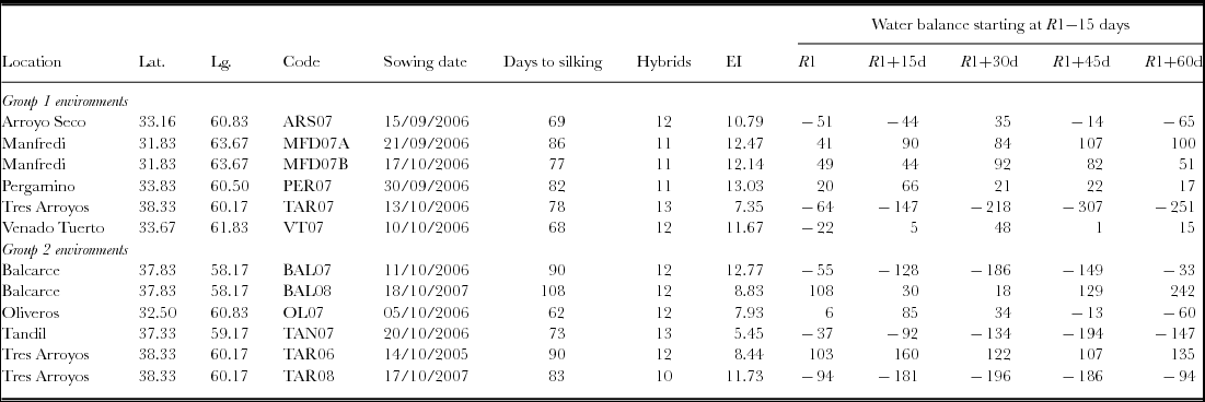
Once all locations satisfying these requirements were gathered, we selected those with the highest number of common hybrids, resulting in 11 locations × 22 hybrids for AFA11, 11 locations × 20 hybrids for AFA12 and AFA13 – Supplementary Material Table S1 (available online at https://doi.org/10.1017/S0014479718000285) – and 12 locations × 13 hybrids for INTA (Table 1). The genotypes compared in each dataset were commercial maize hybrids developed by at least eight different seed companies and, according to the National Register of Cultivars of INASE (National Seed Institute of Argentina, https://www.inase.gov.ar/consultaGestion/gestiones), released within 5 years at most (except for NK900 in the AFA12 dataset) (Tables 2 and S2). Some hybrids were absent from a few environments; when this happened, the missing environments never corresponded to extreme ones (all the hybrids were present in the environments with highest and lowest average yields).
Basic data of each environment (location × year) in INTA trials: latitude (Lat.), longitude (Lg.), code, sowing date, mean days to silking, number of hybrids tested, environmental index (EI, Mg ha−1) and water balance calculations (mm, negative signs indicate water deficit) for the reproductive period starting at R1−15 days. Environments were divided into two groups on the basis of the relation between the environmental index and the water balance at different reproductive periods.

Data analyses
Each dataset was analysed independently. For each hybrid, a maximum and a minimum Y was identified (hereafter, Y max and Y min), which corresponded to the maximum and minimum Y detected across all the field trials of each dataset. For each environment, an environmental index (EI) was calculated as the average Y of all the hybrids present in that environment (i.e., location or location × year).
Yield stability of a hybrid may be assessed by different approaches, such as: (a) the slope (b) of the linear regression between grain Y and EI (Finlay and Wilkinson, Reference Finlay and Wilkinson1963); (b) the estimated variance of genotype deviations from regressions (S2d) (Eberhart and Russell, Reference Eberhart and Russell1966) or (c) the coefficient of variation (CV) for Y across locations (Francis and Kannenberg, Reference Francis and Kannenberg1978). Each approach represents different concepts of stability; we choose the approach (c) for several reasons: (i) it integrates both the unpredictable variations in the response to the environment and the stability across environments; (ii) it is independent on the hybrid average Y; (iii) it is recommended for assessing stability over an entire range of environments (Lin et al., Reference Lin, Binns and Lefkovitch1986) and (iv) there is relatively low variation in the adjustment of fitted regressions among genotypes (there were significant p values for the relation Y vs. EI, as shown in Tables 2 and S2), discouraging the use of other approaches, such as the Wricke's ecovalence analyses (Lin et al., Reference Lin, Binns and Lefkovitch1986). With this approach, Y stability was calculated as
 $$\begin{equation}
{\rm{C}}{{\rm{V}}_i} = \frac{{\sqrt {\frac{1}{{E - 1}}\mathop \sum \nolimits_{J = 1}^E {{\left( {{y_{ij}}\ - {y_i}} \right)}^2}} }}{{{y_i}}}100\% ,
\end{equation}$$
where CVi is the coefficient of variation of the ‘i’ hybrid, E represents de number of environments where it is present, yij is the Y of the ‘i’ hybrid in the ‘j’ environment and yi represents the average Y of the ‘i’ hybrid across environments.
In each dataset and for each hybrid, a cross-over point (CPi) with the 1:1 relation of Y vs. EI was calculated as
 $$\begin{equation}
{\rm{C}}{{\rm{P}}_i} = \frac{a}{{\left( {1 - b} \right)}},
\end{equation}$$
where ‘CPi’ is the cross-over point of the ‘i’ hybrid (a value of EI where hybrid Y changes from being better to being worse than the average of the hybrids in the dataset), and ‘b’ and ‘a’ are the slope and the intercept, respectively, of the relation between Y and EI for that hybrid.
For those hybrids whose Y at the environment with highest EI is lower than the EI, Y performance below the CPi denotes better Y than the average and Y performance above the CPi denotes worse Y than the average. The opposite applies for hybrids whose Y at the highest-yielding environment is higher than the EI. For those hybrids having consistently better or lower Y than the average across the entire environmental range, the CPi values obtained will fall above or below the EI explored in the dataset, and are not shown in Figure 4.
Water balance calculations and environments grouping
For the INTA dataset, an average gross water balance (WB) starting at R1−15 days was calculated as the difference between cumulative rainfall (rf) and PET:
 $$\begin{equation}
{\rm{WB}} = \ \sum\limits_n^{R1 - 15\;{\rm{days}}} {{\rm{rf}}} - \sum\limits_n^{R1 - 15\;{\rm{days}}} {{\rm{PET}}} ,
\end{equation}$$
where ‘n’ are different phenological periods: R1, R1+15 days, R1+30 days, R1+45 days and R1+ 60 days, and R1 corresponds to the average silking date of the hybrids tested in each environment.
In order to assess the existence of ‘cross-tolerance’ to stress, environments were divided into two groups of six: Group 1, where Y was highly determined by (deficient or adequate) WB and Group 2, where Y was determined by many factors, which may involve WB or not. With this approach, Group 1 included environments combining both high water availability and high Y and low water availability and low Y, while environments belonging to Group 2 may have had positive WB combined with low Y because other factors may have been playing the major role in Y achievement. A program was designed in the python 3 language (Van Rossum, Reference Van Rossum2007) in order to obtain all the possible combinations of the 12 environments into groups of 6 (924) that yield the best r 2 in each phenological period. With this approach, the best r 2 (0.93) was obtained for environments shown as group 1 in Figure 4, when EI was regressed by WB during the critical period.
Statistical analyses
Data were evaluated with the STATISTICA 7.1 software (StatSoft, Inc.). Relationships among variables were analysed through linear regressions. In each regression, the r 2 coefficient, the intercept and the slope were calculated and the F-test was used to assess their significance at *p < 0.05, **p < 0.01 and ***p < 0.001.
RESULTS
Relatively high yields in low-yielding environments did not relate to maximum yields but to high Y stability
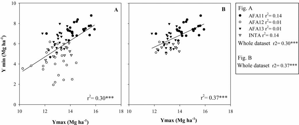
The EI varied widely in each dataset; differences between the best and the worst-yielding environment were 6.6, 8.7, 5.6 and 7.4 Mg ha−1 for AFA11, AFA12, AFA13 and INTA, respectively (Tables 1 and S1). Genotypic variability for Y max and Y min also varied depending on the dataset: the CV for Y max ranged from 3.5% in AFA13 to 8.0% in AFA12, whereas it ranged from 7.7% in AFA11 to 29% in AFA12 (see the scattering of points in both axes in Figure 1A). Overall, the largest difference between Y max and Y min and the largest genotypic variation for both Y max and Y min were detected in the AFA12 dataset. Assuming that improved Y max results in a Y advantage in environments with enhanced stress intensity, a positive relation could be expected between Y max (related to Y potential) and Y min (related to stress tolerance). However, Y max and Y min were not related within each dataset (r 2 < 0.15, Figure 1A) though a trend was detected across them (r 2 = 0.30**, n = 75, Figure 1A). This trend across datasets was reinforced when only Y min higher than 5 Mg ha−1 (usually, the range of expected yields in environments for where breeding is targeted) were considered (r 2 = 0.37**, n = 53, Figure 1B). Nonetheless, since each dataset involved different locations and hybrids, it was not possible to make a statistical comparison among environments to conclude if this trend indicated a genuine relation between Y max and Y min, or if, instead, it was related to intrinsic differences among the datasets.
Correlation between maximum (Y max) and minimum (Y min) yields obtained for each hybrid in the environmental range explored in each dataset (A, n = 75) and the same correlation when only Y min > 5 Mg ha−1 are considered (B, n = 53). Different symbols denote each dataset: AFA11 (black circles, n = 22), AFA12 (white circles, n = 20), AFA13 (black triangles, n = 19) and INTA (white triangles, n = 13); r 2 values obtained for each data set (A) or in the whole dataset (A and B) are shown. *p < 0.05; **p < 0.01; ***p < 0.001.

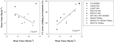
Across datasets, the highest average Y max was reached in AFA11 (14.5 Mg ha−1, p < 0.05), while the lowest Y min was obtained in AFA12 (3.92 Mg ha−1, p < 0.05). Both datasets were pooled together in order to expand the range of Y min and Y max (a difference of 10.4 Mg ha−1 between the highest and the lowest-yielding environment), resulting in nine common hybrids across 22 environments (locations and years). In this combined dataset, a negative relation was detected between mean Y max (average of the three best-yielding environments) and mean Y min (averaged of the three worst-yielding environments) (Figure 2A, r 2 = 0.41, p = 0.06). Enhanced Y max was related to increased unpredictability (assessed through the CV) of yields in low-yielding environments (Figure 2B, r 2 = 0.63, p < 0.01).
Correlation between yields averaged across the three best environments (mean Y max) and yields averaged across the three worst environments (mean Y min) (A, n = 9) and between the ( (CV, %) in the three lowest-yielding environments and mean Y max (B, n = 9), for the dataset obtained after pooling together AFA11 and AFA12 (nine hybrids × 22 locations). Two versions of the hybrids I887 (MG, resistant to lepidopter and MGRR2, also glyphosate resistant) and NK900 (TG, glyphosate resistant and TDMax, resistant to lepidopter) were used in 2011 and 2012 but these differences were considered not important because of effective control of weeds and pests. Each symbol denotes a different hybrid. *p < 0.05; **p < 0.01.

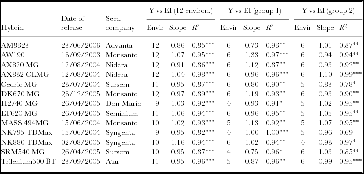
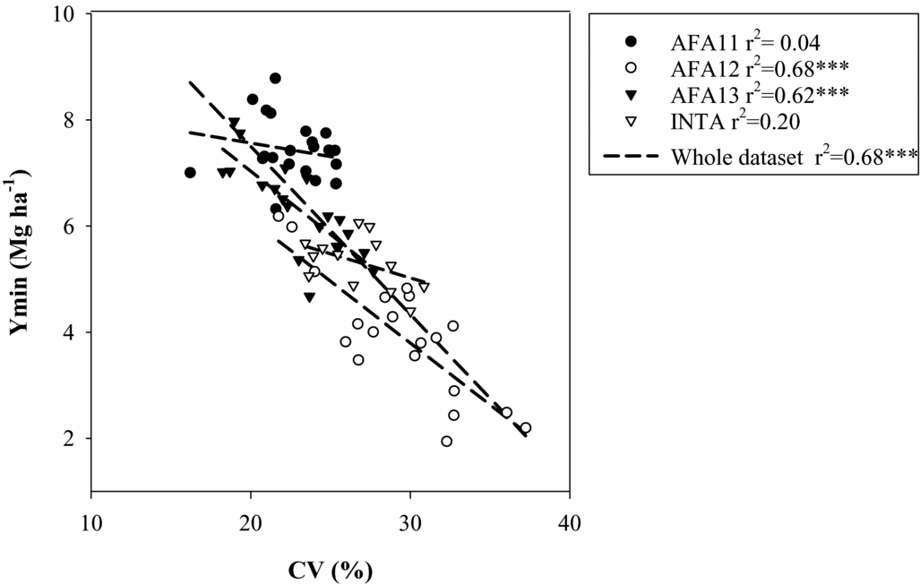
As expected, Y of each hybrid related positively and significantly to the EI explored in each dataset (r 2 > 0.68; r 2 > 0.82; r 2 > 0.78 and r 2 > 0.82 for all hybrids of AFA11, AFA12, AFA13 and INTA datasets, respectively, Tables 2 and S2). However, the slope of the regression varied widely among hybrids, ranging 0.55–1.19, 0.78–1.24, 0.85–1.17 and 0.86–1.16 for AFA11, AFA12, AFA13 and INTA, respectively (Tables 2 and S2). Across datasets, Y min correlated negatively with the CV (r 2 = 0.68***, Figure 3), i.e., Y min correlated with Y stability. Within each dataset, hybrid differences for the CV were more pronounced in AFA12 and AFA13, and concomitantly, better relations between Y min and CV were obtained (r 2 = 0.68*** and r 2 = 0.62***, respectively).
Basic information of each hybrid included in INTA data series: complete name, date of release (day/month/year), Seed Company, number of environments where it was tested (Envir.) and parameters (slope and r 2 coefficient) obtained from the relation between yield (Y) vs. environmental index (EI, Mg ha−1) across all the environments (12), the 6 environments belonging to group 1 (with high relation between yield and the water balance during the critical period) and the 6 environments of group 2 (where yield was not strongly related to the water balance). Asterisks denote p according to the F-test: ***p < 0.001; **p < 0.01; *p < 0.05; +p < 0.1.

Correlation between the coefficient of variation (CV, %) and the Y min obtained for each hybrid in the environmental range explored within each dataset. Solid lines denote the linear adjustment of each dataset and the dashed line shows the linear adjustment for the whole dataset. Different symbols denote the dataset: AFA11 (black circles, n = 22), AFA12 (white circles, n = 20), AFA13 (black triangles, n = 19) and INTA (white triangles, n = 13); r 2 values obtained for each data set or in the whole dataset are shown. *p < 0.05; **p < 0.01; ***p < 0.001.

The relative advantage of hybrids varied across environments
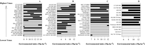
While the relative performance of a hybrid in high-yielding environments may not predict its performance in low-yielding environments (Figures 1 and 2), it might be the case that high Y max predicts a Y advantage across a wide range of moderate-yielding environments. We calculated the cross-over point which defines the performance of a particular hybrid relative to the average (Figure 4). Depending on the dataset, most hybrids had a consistent Y advantage or disadvantage compared with the average (1:1 relation of Y vs. EI) in all the environments explored in their dataset (59% and 60% of the hybrids in AFA13 and INTA, Figure 4C and D) or, on the contrary, most hybrids had a different performance depending on the environment (59% and 70% of the hybrids in AFA11 and AFA12, Figure 4A and B). Particularly for the AFA12 dataset, hybrids with high Y max had a better performance than the average in high to moderate-yielding environments whereas in moderate to low-yielding environments, seven out of the ten hybrids presenting lower Y max had a better performance than the average (Figure 4B).
Yield cross-over point for each hybrid relative to the average of all hybrids (i.e., the environmental index, EI) in each dataset: AFA11 (A), AFA12 (B), AFA13 (C) and INTA (D). Black bars denote the range of EIs where yield of a hybrid is higher than the average, while white bars denote yields lower than the average. The extension of the horizontal axis corresponds to the range of EIs explored in each dataset. Bars of a single colour denote those hybrids for which no cross-over point was detected along the range of explored EIs in each dataset (i.e., having consistently worse or better performance than the average across the range of EIs explored). For each dataset, different hybrids are ordered according to their maximum yield (Y max).

Stability in water-limited environments did not relate to stability in environments exposed to other types of stress
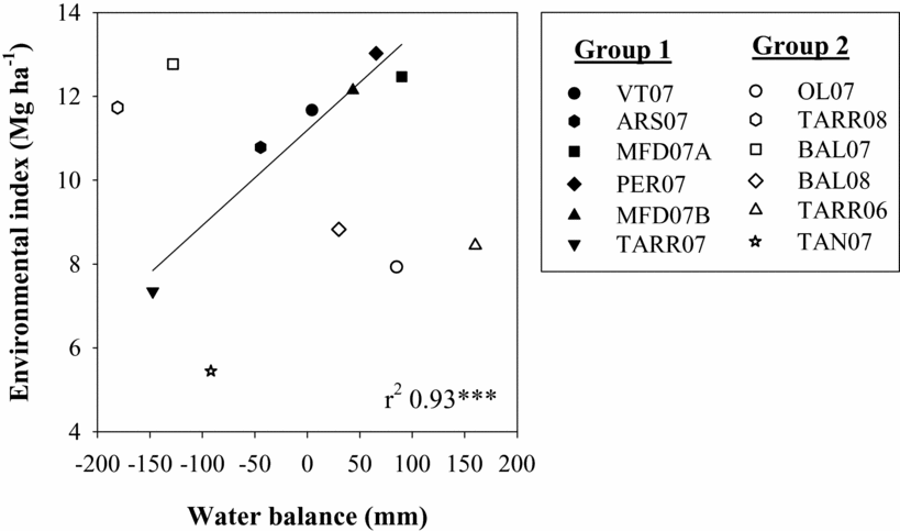
In 6 of the 12 environments of INTA trials (Group 1), the EI was mainly explained by the WB during the critical period (from R1−15 days to R1 +15 days, r 2 = 0.93***) (Figure 5), and other reproductive stages (R1−15 to R1, r 2 = 0.64, p < 0.06; R1−15 to R1+30 days, r 2 = 0.83*; R1−15 to R1+45 days, r 2 = 0.89**; R1 to R1+60 days, r 2 = 0.90**). In the remaining six environments (Group 2), the EI was at least 25% lower or higher than the predicted EI on the basis of the WB and the fitted linear equation obtained for group 1 (Table 1 and Figure 5). The relative performance of the hybrids in these two groups of environments was analysed in order to assess drought stress tolerance during the critical period (in Group 1) or alternatively, tolerance to other types of stress (in Group 2) and the relationship (cross-tolerance) between them.
Correlation between water balance (WB) during the critical period (from R1−15 days to R1+15 days) and the environmental index (EI) in different environments of the INTA dataset. Environments were divided into two groups using a program which tested all possible combinations of the 12 environments in groups of six, and selected the one which yielded the best r 2 for the relation EI vs. WB. Full symbols correspond to Group 1, where WB explains a large part of the yield variation. Empty symbols correspond to Group 2 environments, where a large part of yield variation is not related to WB, and are not included in the linear regression. ***p < 0.001.

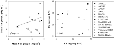
Hybrid average Y for Group 1 environments related positively to average Y for Group 2 environments, when two hybrids were excluded from the regression (r 2 = 0.64**, Figure 6A), but no relation was found when only the worst-yielding environments of each group, i.e., those with the most severe stress intensity, were considered (r 2 = 0.08, data not shown). In the same line, no trace of cross-tolerance was detected considering that Y stability of each hybrid in one group of environments (e.g., group 1 dominated by WB) was not related to stability in the other group, either if stability was assessed by the CV (r 2 = 0.07, Figure 6B) or by the slope of the response of Y to EI (r 2 < 0.005, data not shown). For some hybrids, average yields and Y stability were consistently low (NK795) or high (AX882) in both groups of environments. Other hybrids had a better performance (Y and stability) under environments exposed to other types of stress (AX820-DK670) or conversely, under water-limited environments (LT620, H2740).
Correlation between hybrid average yields in Group 1 and Group 2 environments (A) and between yield stability assessed through the coefficient of variation (CV, B) in the two groups of environments: Group 1 (6 environments), where water balance in the critical period explains a large part of yield, and Group 2 (6 environments), where it does not. Complete names of the hybrids are provided in Table 2. **p < 0.01.

DISCUSSION
Highest yields in low-yielding environments do not relate to maximum yields but to high Y stability
The lack of a consistent relationship between Y max and Y min obtained within each dataset (Figure 1) reinforces the idea that a high potential Y is not a good predictor of Y in stressful environments (Cirilo et al., Reference Cirilo, Dardanelli, Balzarini, Andrade, Cantarero, Luque and Pedrol2009; Monneveux et al., Reference Monneveux, Sánchez, Beck and Edmeades2006; Vadez et al., Reference Vadez, Krishnamurthy, Hash, Upadhyaya and Borrell2011). This is consistent with the presence of specific adaptations that are expressed only under stress (Monneveux et al., Reference Monneveux, Sánchez, Beck and Edmeades2006; Richards et al., Reference Richards, Rebetzke, Condon and van Herwaarden2002). Bänziger et al. (Reference Bänziger, Setimela, Hodson and Vivek2006) reported that maize hybrids bred by CIMMYT in drought environments of Africa had a Y advantage of 40% in environments with average yields of 1 Mg ha−1 compared with hybrids of the private sector (bred in more favourable environments), though this advantage was reduced to 2.5% in environments with average yields of 10 Mg ha−1. Moreover, extending the range of environments tested by combining datasets AFA11 and AFA12 resulted in a negative relation between Y max and Y min (Figure 2A). This is not surprising considering that many traits involved in stress tolerance (e.g., for drought, reduced leaf area, early maturity and prolonged stomatal closure) imply, at the same time, penalties to potential Y (Cattivelli et al., Reference Cattivelli, Rizza, Badeck, Mazzucotelli, Mastrangelo, Francia, Mare, Tondelli and Stanca2008). In this line, Presterl et al. (Reference Presterl, Groh, Landbeck, Seitz, Schmidt and Geiger2002) reported that Y in environments with reduced N availability was higher in those genotypes that were bred in low N environments compared with others bred in favourable environments. In other words, breeding in high-yielding environments may imply discarding genotypes potentially useful for stress-prone areas. While it must not be disregarded that commercial breeding programs are not targeted to low-yielding environments because expected yields do not pay the seed cost, the frequency of occurrence of low Y in high-yielding environments is high enough to increase efforts for improving Y stability. For example, between the 2008 and 2011 maize campaigns, 30 of the 50 departments of Buenos Aires, representing 89% of the area sown with maize in the province, had yields below 5 Mg ha−1 in at least one of those years (http://www.agroindustria.gob.ar). Besides, our results highlight the importance of alternative breeding programs (e.g., from the public sector) destined for stress-prone areas, which, otherwise, are marginalized from breeding improvement.
Results obtained here also suggest that the Y max vs. Y min relationship is likely to be influenced by attributes of the dataset, such as: (i) the amplitude of the range between Y max and Y min, (ii) the absolute values achieved in high and low-yielding environments, and (iii) the genotypic variability expressed in both types of environments which, in turn, may depend on the main stress factor implicated in Y reduction at the lowest-yielding environment. Additionally, it must be noticed that all the trials included in this work were carried out under relatively standardized conditions (conventional fertilisation and weeds and pests controlled), which may have reduced the occurrence of unpredictable responses to the environment, and the genotypic variation associated to it. This may differ from comparisons made on the basis of participative breeding programs, such as the ones developed by CIMMYT in Africa with resource-constrained farmers, where biotic stress tolerance may have also been improved. The relation detected between Y min and CV (Figure 3) together with the lack of a consistent relation between Y max and CV (r 2 < 0.03, data not shown) suggest that Y stability does not necessarily imply penalties to potential Y, but it does imply advantages for Y under stress.
The relative advantage of hybrids varies across environments
The occurrence of cross-over points with the 1:1 relation between Y and EI in many hybrids (Figure 4) shows that it is necessary to know not only the potential Y of a genotype but also its stability across an environmental range in order to evaluate which hybrids perform better under each type of target environment. Agricultural environments can become quite stressful in some seasons. In the 2013/14 maize season in Buenos Aires and Córdoba (provinces representing 57% of the surface sown with maize in Argentina), the average Y was lower than 7 Mg ha−1 (www.siia.gob.ar), and below the EI where most of the cross-over points are found in the present work (Figure 4).
The relatively low occurrence of cross-over points in AFA13 and INTA datasets may be accounted for by different reasons: for AFA13, it may be due to a shorter range between Y min and Y max compared with the rest of the datasets. By contrast, for INTA, hybrids included in the dataset were strictly those consistently repeated in a wide range of years and locations. This may have led, possibly, to an undesired bias towards hybrids with relatively high Y stability, reducing the occurrence of cross-over points.
Stability across environments limited by water deficit during the critical period does not relate to stability across environments exposed to other types of stress
The selection of hybrids with better yields under multifactorial stress may be effective if there is cross-tolerance to stress in the majority of the hybrids (Bänziger et al., Reference Bänziger, Edmeades and Lafitte1999), otherwise, the relative performance of the hybrids will vary depending on the main factor leading to Y reduction. In the present work, no relationship was detected for Y min or CV between both groups of environments (Figure 6B). The diverse combinations for Y stability under both groups (hybrids with high or low Y stability under water-limited environments combined with high or low Y stability under environments exposed to other types of stress) also contrast with the idea of cross-tolerance. The concept of cross-tolerance was proposed on the basis of results obtained from maize populations bred by recurrent selection cycles under drought and tested under N limited environments (Bänziger et al., Reference Bänziger, Edmeades and Lafitte1999). Depending on the stress factors compared, there may be a high relation between the physiological traits leading to Y in different stressful environments (i.e., an extended root system may be desirable under drought as well as under N limitations), which could be expressed as cross-tolerance to stress. In the present work, Y stress tolerance in Group 2 environments (presumably not exposed to nutrient limitations since all the trials were fertilized) is poorly explained by traits leading to Y advantages under drought (Group 1 environments). In any case, a larger number of hybrids and stressful environments should be analysed to strengthen these observations. If cross-tolerance is not the rule, then, a more accurate analysis of Y stability could be done by making a previous selection of environments with a main stress factor in common to avoid non-informative dispersion of data.
CONCLUDING REMARKS
Tollenaar and Lee (Reference Tollenaar and Lee2002) reported average record maize yields of about 20 Mg ha−1 for central North America, which are three times larger than the average commercial maize yields in Argentina obtained in 2013/14 (www.siia.gob.ar). Besides, climate change, soil degradation and the expansion of the agricultural frontier to marginal zones (Fedoroff et al., Reference Fedoroff, Battisti, Beachy, Cooper, Fischhoff, Hodges, Knauf, Lobell, Mazur, Molden, Reynolds, Ronald, Rosegrant, Sanchez, Vonshak and Zhu2010) forecast an increasing occurrence of unpredictable stress. To make things worse, maize Y increases in the last years have been associated to a higher sensitivity to water stress (Lobell et al., Reference Lobell, Roberts, Schlenker, Braun, Little, Rejesus and Hammer2015). If, as shown in the present work, there is not a consistent relation between potential Y and stress tolerance, increasing Y potential may not necessarily represent a useful strategy to improve maize Y in farmers’ fields. The occurrence of cross-over points in the rather short range of environmental indexes analysed shows that maize hybrids with moderately or high potential Y are not always the best choice in moderate and low-yielding environments and highlights the use of Y stability in order to assess the suitability of hybrids for particular environments. Finally, our results suggest poor cross-tolerance for different types of stress in the largest part of the hybrids, though further research is needed to strengthen this conclusion.
Acknowledgements
This work was funded by PICT 2012-1862. We thank Lic. Ana Teresa Gómez from Servicio Meteorológico Nacional for providing us the meteorological data for INTA locations. We are also thankful to Dr. Hernán Sánchez (CONICET, IFLySiB) for designing the program for grouping environments with python. We appreciate advice on statistical analyses from Dr. C. Graciano and thoughtful suggestions on the manuscript from Dr. E. A. Tambussi and Dr. M. Maydup. M. A. and J. J. G. are researchers of CONICET.
SUPPLEMENTARY MATERIAL
To view supplementary material for this article, please visit https://doi.org/10.1017/S0014479718000285