1. Introduction

We describe two anomalies in Bohm’s theory. In both anomalies the theory implies that particles can arrive into regions of the configuration space in which the wave function is zero, and therefore the motion is not well defined. The first anomaly arises in a spin measurement on a single particle by means of a Stern-Gerlach magnet. The second arises in Stern-Gerlach measurements on Einstein-Podolsky-Rosen/Bohm pairs of particles where the measurements are simultaneous in the preferred frame of reference. Both anomalies pertain to conditions that are allowed by Bohm’s theory but have measure zero. In this sense, measure (or probability) zero means in Bohm’s theory unlikelihood but not strict impossibility. By contrast, in standard quantum mechanics (QM) in the above conditions probability zero means strict impossibility, in the sense that the events in question do not belong to the space of all possible events. The anomalies are states of affairs that are unlikely by Bohm’s theory but strictly forbidden by standard QM.

2. A Stern-Gerlach Measurement

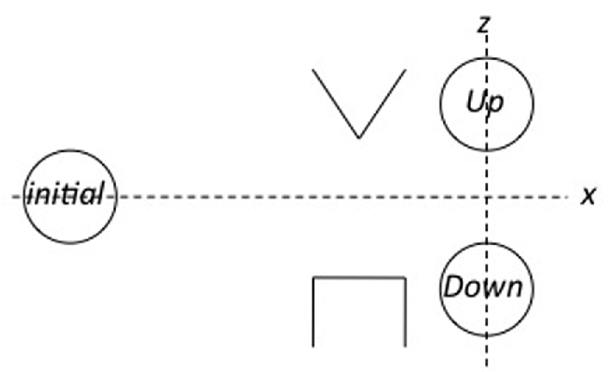
Consider a Stern-Gerlach measurement of the spin in the z-direction of a spin-1/2 particle prepared in the up eigenstate of spin in the x-direction (see fig. 1). The initial quantum state of the particle is a product state of the spin degree of freedom and the wave function:

where corresponds to the up eigenstate of the x-spin, and is the wave function of the particle that we assume moves to the right and that is taken ideally to be nonzero only in the region of space L. The interaction of the particle with the magnetic field results in coupling its wave function to the up and down eigenstates of the z-spin. The wave function evolves into two components and that move, respectively, in the upward and the downward directions and that have nonzero amplitudes only in these regions. When the two wave functions separate completely in space, the quantum state of the particle becomes

such that the z+ and z− eigenstates of the z-spin are one-to-one correlated with, respectively, the upward and the downward wave functions.

Figure 1.

Stern-Gerlach experiment.

Standard QM predicts that the outcome of the measurement will correspond to z+ or z− with probability 1/2. This is expressed in standard QM by von Neumann’s collapse postulate according to which the state (2) is replaced after the measurement with one of the components in (2) (normalized) corresponding to the outcome obtained. The events space corresponding to the possible outcomes consists only of the two outcomes z+ and z−, and the event that a subsequent position measurement will find the particle anywhere else after the measurement has probability zero. We suggest that in standard QM this probability zero should naturally be understood as strict impossibility, in the sense that this event does not belong to the space of all possible events. This point will turn out to be important since, in Bohm’s theory, probability zero in this context has a different meaning, as we will see in sections 3 and 5.

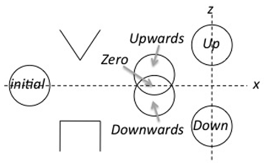
In Bohm’s theory, the outcome of the measurement is determined by the position of the particle, which changes according to its trajectory as given by the velocity equation (see fig. 2).Footnote ¹ Initially, in state (1) the particle may be located anywhere in the region where the amplitude of the initial wave function is nonzero, and the probability that it is located at a point x in that region is given by at that point. In Bohmian mechanics, when we say that the particle is prepared exactly in the x-spin-up eigenstate, we mean that the initial wave function is symmetrical with respect to the z-axis in two different senses. First, if the zero point on the z-axis is taken to be the middle of the magnetic field, then the probability that the particle is located above or below this zero point is equal to 1/2. Second, the velocity of the particle in the z-direction as determined by the z-component of is zero for all the positions in L.

Figure 2.

Bohmian account of Stern-Gerlach experiment.

In the region of interaction with the magnetic field, the wave function evolves such that its amplitudes are nonzero in three subregions that we call upward, downward, and zero regions as follows: positions in the upward region evolve by the velocity equation upward relative to the z-axis, positions in the downward region evolve by the velocity equation downward, and positions in the zero region have zero velocity in the z-direction. If the particle happens to be anywhere in the upward region (i.e., in a position where only the amplitude of the upward wave function is nonzero), then according to the velocity equation, the symmetry of the wave function breaks, and the particle will assume an upward velocity. Similarly, if the particle happens to be in the downward region, then it will assume a downward velocity. And as long as the particle happens to be located in the zero region, its velocity in the z-direction remains zero. The wave function evolves in space such that positions that previously belonged to the zero region gradually become part of the growing upward or downward regions. And so eventually the particle is trapped in either the upward region or the downward region, depending on its initial position, and is then carried along with the flows of the amplitudes in that region according to the velocity equation.

This means that the initial positions within the initial wave function are divided into two sets, which we call an up set and a down set, such that all the points in the up set will deterministically evolve by the velocity equation into the upward region of the wave function, and all the points in the down set will evolve into the downward region.

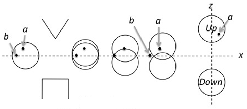
However, it is known that there is an anomalous situation. Consider two points a and b both of which belong initially to the zero region (see fig. 3). The point b is located exactly on the zero point in the z-direction. When the particle approaches the magnetic field the wave function evolves such that point a is first located on the line separating the zero region and the upward region and subsequently it is trapped in the upward region. Point b by contrast is first located on the “tangent” of both the upward and the downward regions, and therefore it will subsequently belong to neither region. This means that if the particle is located initially at point b it will subsequently be located in regions of space in which the amplitude of the wave function is zero. Nothing in Bohm’s theory precludes points such as b from being in the set of possible initial positions. This means that positions in the region in which the wave function is zero are possible by the dynamics. But in such regions it seems that the dynamics breaks down since the motion of the particle is ill defined (and likewise all other properties, except position).Footnote ² Of course, the probability given by the absolute square of the amplitude that the particle will sit on the b points is zero. However, this zero probability does not imply impossibility since the anomalous b points are included in the events space.Footnote ³ We expand on this point in section 5. Note that in realistic situations both QM and Bohm’s theory agree that the probability that the particle will hit the screen in the middle is nonzero due to the tails of the wave function. But in our case, the tails are zero by assumption.

Figure 3.

Anomalous case.

3. Spacelike Separated Spin Measurements

Consider two particles with spins prepared in the quantum mechanical singlet state:

where and are the eigenstates of the z-spin of each of the particles. Suppose that the particles are sent off to spacelike separated regions, and we measure spin in the z-direction on each of them by means of Stern-Gerlach magnetic fields. Before the interaction with the magnetic fields, the complete quantum state of the two particles including their spatial wave functions is

where is the wave function of particle 1, which moves to the left, and is the wave function of particle 2, which moves to the right. In (4) the wave functions of the two particles are separable, although, of course, the spin parts of the two particles are nonseparable. After the interactions with the magnetic fields on the two wings of the experiment, the quantum state becomes

in which the z-spin of each of the particles is coupled to the upward and downward wave functions such that also the wave functions of the two particles become nonseparable.

Standard QM predicts that the joint outcomes of these measurements will be either (z+, z−) or (z−, z+) with probability of exactly 1/2, as calculated by the Born rule. Any other joint outcome, for example, (z+, z+) and (z−, z−), is given by this algorithm probability zero. Similarly to the single case, we suggest that this zero probability should be understood as implying that when the two particles are in state (4) immediately before the measurements, the joint measurement outcomes (z+, z+) and (z−, z−) are strictly impossible and do not belong to the events space of possible joint outcomes (see also sec. 5). The reason is that the correlated states

and

are both orthogonal to the state (5), and there is no transformation from (5) to either (6) or (7)—neither by the unitary Schrödinger equation nor by von Neumann’s projection postulate.

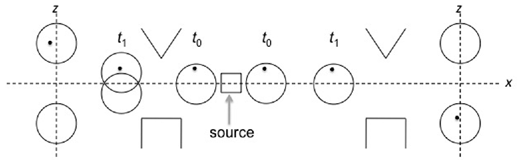
The account given by Bohmian mechanics to the same experiment (see fig. 4) is significantly different. As in the single Stern-Gerlach experiment described above, the joint outcome of this experiment is determined by the evolution of the wave function and the trajectories of the two particles under the influence of the magnetic fields. Each of the two wave functions and ends up in a quantum mechanical (improper) mixture of an upward and a downward component, where each component induces (respectively) an upward or a downward velocity on each particle.

Figure 4.

Bohmian account of Einstein-Podolsky-Rosen/Bohm experiment with a nonsimultaneous up-up pair.

Since the two initial wave functions are separable in (4), the probability distributions over the positions of the two particles are independent of each other. This means that the space of all the possible initial positions for the two particles consists of the following sets: the set (up, up) of all initial positions such that will induce an upward velocity on particle 1, and will induce an upward velocity on particle 2; and the set (up, down) consists of all initial positions such that will induce an upward velocity on particle 1, and will induce a downward velocity on particle 2; and similarly for the sets of pairs of positions and induced velocities (down, up) and (down, down). These four sets of the two-particle positions have equal weights of 1/4, which can be described in terms of probability, since the probability that a position measurement will find the particles in positions that belong to each of these sets is equal to 1/4.Footnote ⁴ In this picture the (up, up) set and the (down, down) set, taken together, have quantum probability measure of 1/2. In this sense the structure of the events space of the two-particle system in Bohmian mechanics is essentially the same as that of the setup described by a classical statistical mechanical model in which two fair coins are tossed. The only (albeit significant) difference is that in the classical case of the two coins the probabilities for joint outcomes are 1/4 for each combination of heads and tails, whereas in the singlet state the probabilities for the outcomes (z+, z+) and (z−, z−) corresponding to the joint initial positions (up, up) and (down, down) are zero.

Of course, Bohm’s theory must assign probability zero to these outcomes, if it is to be empirically equivalent to QM. But since as we just saw the correlated positions (up, up) and (down, down) have quantum measure 1/2 in the initial configuration space, the question arises why trajectories that would yield the outcomes (z+, z+), (z−, z−) have zero probability. Suppose that the positions of the two particles in state (4) are in the (up, up) set, and let the first measurement be carried out on particle 1 (see fig. 4).Footnote ⁵

It follows from the analysis of the Stern-Gerlach measurement in the single particle case that when the wave function of particle 1 splits into the upward and the downward moving wave functions in the Stern-Gerlach magnetic field on the left, the particle will be trapped in , and therefore the velocity of particle 1 as dictated by the velocity equation is bound to be in the upward direction; that is, particle 1 will evolve along regions of space in which the amplitude of the upward moving wave function is nonzero and in which the amplitude of the downward moving wave function is zero. And since the wave functions of the two particles in (5) are nonseparable, this also means that (effectively) the second component of the superposition in (5) receives instantly and nonlocally zero amplitude at the point at which particle 2 is located. In the velocity equation this means that the superposition effectively collapses onto the left component. Therefore, particle 2 is bound to move subsequently downward independently of its initial up-set position. And so the outcome of the second measurement, on the right, will be z− with certainty, just as standard QM predicts. And again we see that the probability that a subsequent position measurement will find particle 1 in the region covered by the effective wave function, in this case, , is and that a position measurement will find particle 2 in the region covered by is . As before, the quantum mechanical probability distribution over the positions of particles is preserved—in this case due to the nonlocal dynamics in the velocity equation. A similar analysis applies if the positions of the two particles are in the (down, down) set.

4. Bohm’s Theory in the Preferred Frame

The type of nonlocality in the dynamics just described requires an absolute time order and therefore a preferred frame in the context of special relativity. The reason is this. As we saw, the trajectory of the particle that interacts first with the magnetic field is invariably determined by its position in a straightforward way by the currents of the probability amplitudes of the local wave function. But in 1/2 of the runs of the experiment (i.e., whenever the joint positions of the two particles belong to the (up, up) set or the (down, down) set in the wave function) the velocity of the particle that gets measured subsequently is determined nonlocally through the two-particle wave function by the velocity of the remote particle. If we consider a frame in which the measurement on the left is carried out first and suppose that the joint positions are in the (up, up) set, then the left particle will move upward and the outcome of the measurement will be z+, and then subsequently (in this frame) the right particle will move downward and the outcome of the measurement on the right will be z−. But if the same experiment is described in a frame in which the temporal order of the measurements is reversed, then the right particle will move upward and the outcome of the measurement in this second frame will be z+, and then subsequently (in this frame) the left particle will move downward and the outcome of the measurement on the left will be z−.

And if this were true, observers (moving relative to each other) associated with different reference frames would disagree about whether the left particle (for example) hit the up or down region on the screen; that is, different frames would disagree about which measurement outcomes occur in approximately 1/2 of the runs of such experiments. And we know that this is not the case. The only way to avoid this result is to suppose that there is a preferred frame, which determines an absolute time order of spacelike separated events by fixing some absolute standard of simultaneity. This means that the trajectories taken up by the two particles in our setting are fixed once and for all by the absolute temporal order of the measurements in the preferred frame.

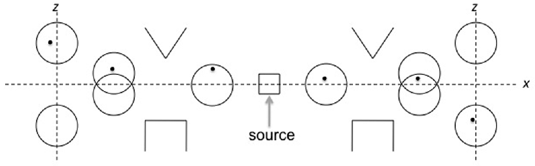
But this has the following implication. Consider again two particles prepared in the singlet state (4) and suppose (as above) that the positions of the particles belong to the (up, up) set (which should be true approximately 1/4 of the time). Suppose further that the particles are located in different positions relative to the z-axis (see fig. 5). Finally, suppose that the measurements on the two wings happen to be simultaneous in the preferred frame. In this case the separation in real three space of the upward and downward wave functions on the two wings of the experiment occurs simultaneously in the preferred frame. But the particle on the left is trapped in the upward region first (in the preferred frame), and therefore the particle on the right will evolve downward regardless of its initial up-set position as we explained above.

Figure 5.

Bohmian account of Einstein-Podolsky-Rosen/Bohm experiment with a simultaneous up-up pair.

However, there is an anomalous situation here too. Suppose not only that the measurements are simultaneous in the preferred frame but also that the particles are located in exactly the same positions relative to the z-axis. In this case the two particles will leave the zero region of the wave function exactly at the same time in the preferred reference frame. Since the measurements are simultaneous in the preferred frame, each particle receives both (as it were) a signal from its local wave function that directs it upward and at the same time a nonlocal (as it were) signal from the remote part of its wave function that directs it downward. In this case, the particles evolve into regions of the six-dimensional configuration space in which the wave function (5) is zero.Footnote ⁶ One may think of this case as if the nonlocal and the local signals cancel out each other in the configuration space so that the particles will have no velocity at all (as opposed to zero velocity in the preferred frame).Footnote ⁷ And therefore Bohm’s theory does not seem to be capable of determining the motion of the particles at these regions in any direction or any other (contextual) property. If one does not want to say that the theory breaks down, one must explain how velocity is determined in this case.Footnote ⁸

Of course, this anomalous situation is not feasible since there is zero probability that the two particles will occupy the same position relative to the z-axis, and even if this should happen by chance, there is zero probability that our measurements on the two wings will be simultaneous in the preferred frame. But nothing in the principles of Bohm’s theory forbids this double coincidence, which is therefore possible. We do not know whether these anomalies reveal a devastating incoherence in the structure of Bohm’s theory. But they are disturbing since they seem to depict conditions at which the dynamics breaks down.

5. Measure Zero

In both anomalous scenarios, Bohm’s theory implies that the particles arrive into regions of space that are strictly forbidden according to standard QM as we understand it. In standard QM we suggested that these events are assigned probability zero in the sense of strict impossibility; that is, the events are considered outside the space of all possible events (and according to QM the anomalies do not arise). By contrast, in Bohm’s theory the set of ‘forbidden’ events has quantum measure zero, but the structure of the theory implies that they exist in the configuration space of the particles; namely, they are not strictly impossible. The situation is essentially the same as in classical statistical mechanics, according to which, for example, the set of initial conditions of an ergodic system that lead to thermodynamically abnormal trajectories must exist in the phase space but has (Lebesgue) measure zero.

We suggested that in standard QM the joint outcomes (z+, z+) and (z−, z−) do not merely have probability zero but rather do not belong to the event space corresponding to the outcomes of the two measurements. Let us now argue for this view.

Consider a particle in an infinite potential well. The probability that a position measurement will find the particle exactly in any particular point x (or a Gaussian centered around this point) is zero, but of course this zero probability does not imply impossibility since after the measurement the particle is located at a point that had zero probability in this sense. Here the sense of probability zero in QM is essentially the same as in classical statistical mechanics. However, the probability that the measurement will find the particle anywhere outside the well is also zero, but in this case the zero probability implies strict impossibility since any position outside the well does not belong to the space of all possible events. It is this second sense of probability zero, we suggested, that features in the standard quantum mechanical account of the spin measurements we described above.

In general, in the theory of probability there is a distinction between the events that do not belong to the event space and those that belong to the space and have probability zero. If one takes the transition from state (5) to state (6) or (7) as possible (although with probability zero), it seems to us that this distinction is blurred. If we want standard QM to respect this distinction, we need to interpret it as we suggested, for the following two reasons.

First, the state vectors corresponding to the correlated outcomes (z+, z+) in (6) and (z−, z−) in (7) are orthogonal to the state immediately before the collapse, namely, state (5), and therefore neither the Schrödinger equation nor von Neumann’s projection postulate can transform (5) into either (6) or (7).

Second, if we add (6) and (7) as components in (5) with amplitude zero, in order to formally apply the projection postulate and the Born rule, this addition has no empirical consequences whatsoever, since according to QM there are no observables that are sensitive to the existence of components in the quantum state that have zero amplitude. Components of the quantum state that have zero amplitude ipso facto have no phase. In this sense such an addition is meaningless. Therefore, it seems to us that according to standard QM it is meaningless to say that although the outcomes (z+, z+) in (6) and (z−, z−) in (7)—or any outcome except (z+, z−) and (z−, z+)—have zero probability, they are still possible. (Note that in classical statistical mechanics, by contrast, points in measure zero sets, that lead to anti-thermodynamic behavior, have empirically significant consequences.)