1. Introduction
Recent studies have stressed the potential effects of environmental policy on market structure and competition, suggesting that environmental regulation hinders entry. In particular, those policies increase the initial investment that firms must incur in order to operate in the industry, such as OECD (2006) and Ryan (Reference Ryan2012),Footnote 1 or allow for economies of scale to emerge in the compliance of environmental policy, ultimately entailing cost differentials between incumbents and entrants.Footnote 2 Nonetheless, to our knowledge, the analysis of how different environmental policy regimes affect entry has been overlooked by the existing literature. In this paper, we identify under which conditions policies that cannot be rapidly adjusted across time, while deterring entry, yield a larger welfare than policies that can be revised over time. Hence, our findings provide guidance for policy makers who regulate polluting industries subject to the threat of entry. Moreover, we show that environmental policies, despite deterring entry, might be opposed by incumbent firms.
Specifically, our study considers a social planner who sets emission fees on an industry, initially monopolized by an incumbent, and where an entrant may decide to join the market afterwards. We examine two given policy regimes that the regulator might face: a flexible policy, in which emission fees can be adjusted if the market structure changes; and an inflexible policy, in which the regulator does not have the ability to rapidly adjust environmental policy, i.e., fixed fee. Several environmental regulations in the US are frequently revised. For instance, EPA (2001) indicates that wastewater discharge fees across most states have been raised approximately every year since 1986, exceeding the rate of inflation. Similarly, air emission fees in California have also experienced yearly changes since 1996. Other environmental policies, however, remain relatively constant across time, such as timber yield taxes and taxes on aviation noise pollution.Footnote 3 , Footnote 4 While our results provide welfare comparisons across regimes, our model does not allow the regulator to modify the policy regime in which he operates.
Under an inflexible policy, initial fees are still enforced in the post-entry game. Therefore, this regulation can attract or deter entry when the regulator sets a relatively low or high fee, respectively. In contrast, when the regulator operates under a flexible policy, he cannot credibly deter entry, since he can revise emission fees if entry ensues. In an inflexible policy, the social planner must select a single emission fee, thereby producing inefficiencies in either one or both periods. We nonetheless show that the regulator can improve social welfare by strategically setting a significantly high fee that deters entry. In particular, relative to a flexible policy, the imposition of a stringent inflexible fee produces two opposite effects: first, it reduces monopoly output during both periods, but second, it generates savings in entry costs and environmental pollution. When the latter effect dominates the former, overall welfare increases, and therefore entry deterrence becomes socially optimal. Otherwise, attracting entry is preferred and a flexible environmental policy yields a larger welfare. Our results hence suggest that countries where environmental regulation slowly adjusts to changes in industry conditions (inflexible regimes) could unintentionally hinder entry, yet they would generate a larger social welfare than by the implementation of policies that attract entry.
Finally, we investigate whether the incumbent's profits are negatively affected by emission fees that deter entry, thus identifying under which conditions the incumbent would actually oppose these entry-deterring fees. An inflexible policy allows the incumbent to maintain its monopoly power, but reduces profits across time. Specifically, we show that, when entry is deterred by setting a high inflexible emission fee, the incumbent's benefits from monopolizing the industry are offset by the costs from bearing this fee, and hence the incumbent would lobby against an inflexible policy. We hence demonstrate that the regulator's and incumbent's interests are not necessarily aligned. In particular, when the regulator finds entry deterrence socially optimal, the incumbent can oppose such a policy if the emission fee it bears is relatively high, i.e., the incumbent may actually prefer that the regulator practices less entry deterrence.
Previous literature has analyzed the effect of environmental policy on firms' profits, such as Porter (Reference Porter1991) and Porter and van der Linde (Reference Porter and van der Linde1995a, Reference Porter and van der Linde1995b), who study how innovation practices are affected by regulation, and Farzin (Reference Farzin2003), who examines the effects of environmental standards on product quality and its associated demand. These studies, however, overlook the entry-deterring consequences of environmental policy on the incumbent's profits.
Moreover, our paper relates to the literature on entry-deterrence games.Footnote 5 Since this literature often abstracts from the regulatory context in which firms operate, entry is only deterred if the incumbent seeks to discourage the newcomer. Our results, in contrast, predict settings where the regulator's practice of entry deterrence is actually opposed by the incumbent firm.Footnote 6
In a related paper, Schoonbeek and de Vries (Reference Schoonbeek and de Vries2009) also consider the role of environmental regulation in deterring entry. However, they assume that environmental policy is initially absent, and becomes only present in posterior stages, as if environmental regulation were newly introduced in that industry. Our model, by contrast, examines markets which were already subject to regulation, i.e., firms facing emission fees in all periods. This time structure gives rise to findings that did not emerge in Schoonbeek and de Vries (Reference Schoonbeek and de Vries2009). In particular, in their article the incumbent firm is willing to bear a one-period stringent fee that deters entry in contexts in which the regulator does not find such a policy welfare improving. Our results, in contrast, show that the incumbent is less willing to bear such entry-deterring regulation during all periods, i.e., this firm actually opposes entry-deterring policies in settings in which the regulator finds welfare improving to deter entry. Hence, our paper suggests that firms in polluting industries that recurrently face environmental regulation will not favor environmental policy, as described in Schoonbeek and de Vries (Reference Schoonbeek and de Vries2009), but instead would actively lobby against such a regulation. Finally, since entry deterrence is only feasible under inflexible policy regimes, we also examine a flexible policy, whereby the regulator can revise emission fees upon entry, providing welfare comparisons between these two regimes.Footnote 7
The next section describes the model and time structure of the game. Section 3 examines the flexible policy regime, while section 4 investigates equilibrium fees under an inflexible policy. Section 5 compares the overall social welfare ensuing from the selection of different environmental policies. Section 6 evaluates the incumbent's profits under flexible and inflexible policies, and section 7 concludes.
2. Model
Consider an entry game with a monopolist incumbent, an entrant who decides whether or not to join the market (incurring an entry cost F) and a regulator who sets an emission fee per unit of output. If entry occurs, firms compete à la Cournot. In addition, firms face an inverse linear demand function p(X) = 1 − X, where X denotes aggregate output. The incumbent's and entrant's constant marginal costs are 0 ≤ c < 1. In particular, we study a two-stage complete-information game with the following time structure:
-
(1) First period:
-
(1a) Under an inflexible policy regime, the regulator sets a constant fee t across time, i.e., non-adjustable fee. Under a flexible policy regime, he sets fee t 1 in the first period, but he is allowed to adjust it to t 2 at the beginning of the second period.
-
(1b) Given the first-period environmental policy, the incumbent responds selecting an output level, i.e., q(t) under an inflexible policy or q(t 1) under a flexible policy.
-
-
(2) Second period:
-
(2a) The entrant decides whether to enter the industry after observing the emission fee and the incumbent's marginal costs.
-
(2b) The regulator maintains his environmental policy t if he operates under an inflexible fee. Otherwise, he revises the policy from t 1 to t 2. In addition:
-
(i) If entry does not occur, the incumbent responds producing a monopoly output x inc NE (t) under an inflexible policy and x inc NE (t 2) under a flexible policy; where subscript inc represents the incumbent, and superscript NE denotes no entry.
-
(ii) If entry ensues, both firms compete as Cournot duopolists, producing x inc E (t) and x ent E (t) under an inflexible policy, and x inc E (t 2) and x ent E (t 2) under a flexible policy; where subscript ent denotes the entrant, and superscript E represents entry.
-
-
In the following section we examine fees and output levels in the flexible policy regime, as well as the resulting social welfare in equilibrium. Afterwards we analyze the inflexible regime, and finally compare social welfare under both policies. In addition, we next describe the demand function firms face and the social welfare function that the regulator uses to set optimal emission fees.
3. Flexible policy regime
3.1. Second-period game
No entry
If entry does not occur, the incumbent's profits when facing an inverse demand function p(x inc ) = 1 − x inc and a given fee t 2 are π inc NE (x inc ) ≡ (1 − x inc ) x inc − (c + t 2) x inc . The regulator's social welfare function in the second period is
 $$SW_{2}^{NE}\equiv CS\lpar x_{inc}\rpar +\pi_{inc}^{NE}\lpar x_{inc}\rpar +T^{NE}-d\times \left(x_{inc}\right)^{2}\comma \;$$
where CS(x
inc
) represents the consumer surplus for a given output x
inc
. In addition, T
NE
is the tax revenue from collecting emission fees under no entry, and d × (x
inc
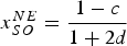
)2 represents the environmental damage from output, where parameter d > 0. The regulator induces the socially optimal output
 $x_{SO}^{NE} = {1 - c \over 1 + 2d}$
by setting emission fee t
2
NE
= (2d − 1)x
SO
NE
, where
 $d \in \left[{1 \over 2}\comma \; 1 \right]$
.Footnote
8
(For further details about equilibrium fees with and without entry, see Appendix 1.)
Entry
If entry occurs, firms compete as Cournot duopolists in the second period, producing an aggregate output of X = x
inc
+ x
ent
. The regulator's social welfare function is SW
2
E
≡ CS(X) + PS(X) + T
E
− d × X
2, where PS(X) ≡ π
inc
E
(x
inc
,x
ent
) + π
ent
E
(x
inc
,x
ent
) − F denotes producer surplus, and F is the fixed entry cost.Footnote
9
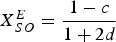
The regulator induces the same aggregate socially optimal output as without entry, i.e.,
 $X_{SO}^{E} = {1 - c \over 1 + 2d}$
.Footnote
10
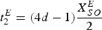
Specifically, the optimal second-period fee is
 $t_{2}^{E} = \lpar 4d - 1\rpar {X_{SO}^E \over 2}$
where t
2
E
> t
2
NE
, illustrating that the regulator sets more stringent fees to the duopolists than to the monopolist, as in Buchanan (Reference Buchanan1969). Finally, note that entry is profitable if emission fees are sufficiently low, but becomes unprofitable otherwise. That is, profit function
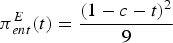 $\pi_{ent}^{E}\lpar t\rpar = {\lpar 1 - c - t\rpar ^2 \over 9}$
originates above F, but falls below it for
 $t\geq \bar{t}$
. For compactness, we refer to
 $\bar{t}$
as the ‘entry-deterring’ fee, which solves π
ent
E
(t) = F, i.e.,
 $\bar{t} = 1 - c - 3 \sqrt{F}$
.Footnote
11
3.2. First-period game
The regulator seeks to induce a first-period output q
SO
that maximizes social welfare, which coincides with x
SO
NE
. Hence, the first-period fee t
1 that induces the monopolist to produce q
SO
coincides with that under no entry in the second period, i.e., t
1 = t
2
NE
. Let SW
E
(t
1,t
2
E
) represent the social welfare when entry occurs and the regulator sets fees t
1 and t
2
E
. In particular, overall social welfare is
 $SW^{E}\left(t_{1}\comma \; t_{2}^{E} \right)= {1 - \lpar 2 - c\rpar c \over 1 + 2d} - F$
.
4. Inflexible policy regime
In the second-period game, firms face the same constant fee t selected in the first period. Hence, we next analyze the regulator's setting of an optimal inflexible policy at the beginning of the game. In the case of no entry, the regulator seeks to induce the same optimal output in both periods, namely, q SO and x SO NE . This can be achieved by a fee t NE , which coincides with the optimal fee t 1 = t 2 NE under a flexible policy. If entry occurs, however, the regulator needs to set different fees to the first-period monopolist from that to the second-period duopolists in order to induce the socially optimal aggregate output. Any fee t that remains constant across time, therefore, produces a deadweight loss in one or both periods. Hence, in this setting the regulator minimizes the sum of the deadweight losses across both periods, choosing a fee t that solves
 $$\mathop{\min}\limits_{t} DWL_{1}\lpar t\rpar + DWL_{2}\lpar t\rpar$$
The deadweight loss in the first period is
 $DWL_{1}\lpar t\rpar \equiv \vint_{q\lpar t\rpar }^{q_{SO}}\lsqb SMB^{NE}\lpar q\rpar - MD^{NE}\lpar q\rpar \rsqb dq$
, where SMB
NE
(q) denotes the social marginal benefit of additional output, MD
NE
(q) represents the marginal environmental damage of output, and
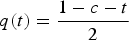 $q\lpar t\rpar = {1 - c - t \over 2}$
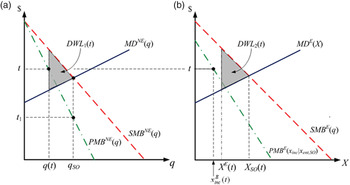
is the monopoly profit-maximizing output for a given fee t. Figure 1a illustrates the first-period welfare loss of setting a fee t that differs from the socially optimal fee t
1. In particular, figure 1 depicts the case where t > t
1, leading to a monopoly output q(t) that lies below the socially optimal output q
SO
. Specifically, q
SO
solves MB
NE
(q) = MD
NE
(q), and the emission fee that induces the monopolist to produce such an output level, t
1, is obtained from solving PMB
NE
(q
SO
) = t, where PMB
NE
(q) represents the incumbent's private marginal benefit of increasing output under no entry. (For further details about equilibrium fees under an inflexible regime, see Appendix 2.)
(a) First-period welfare loss and (b) Second-period welfare loss

Similarly, the deadweight loss associated with tax t in the second period is given by
 $DWL_{2}\lpar t\rpar \equiv \vint_{X^{E}\lpar t\rpar }^{X_{SO}^{E}}\left[SMB^{E}\lpar X\rpar -MD^{E}\lpar X\rpar \right]dX$
, where X
E
(t) = x
inc
E
(t) + x
ent
E
(t) and x
j
E
(t) represents firm j's profit-maximizing output for a given fee t after entry. Deadweight loss DWL
2(t) is depicted in figure 1. Hence, when entry occurs, the optimal tax is a weighted average of first- and second-period taxes,
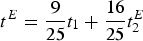 $t^{E} = {9 \over 25} t_{1} + {16 \over 25} t_2^E$
, and thus t
1 < t
E
< t
2
E
. (This fee generates strictly positive production levels for both incumbent and entrant across periods; see Appendix 2 for further details.)Footnote
12
4.1. Entry deterrence
In the context of an inflexible environmental policy, the regulator can select a relatively high fee
 $\bar{t}$
that deters entry, i.e., a fee that lowers the entrant's duopoly profits below his fixed entry cost F. Let
 $SW^{NE}\lpar \bar{t}\rpar $
denote overall social welfare when the regulator sets a fee
 $\bar{t}$
that deters entry. Intuitively, the welfare cost of deterring entry arises from substantially reducing the incumbent's monopoly output across both periods, thereby decreasing consumer surplus and profits, whereas its welfare benefit emerges from the reduction in pollution and the savings in entry costs. In particular, the regulator can deter entry by setting fee
 $\bar{t} = 1 - c - 3 \sqrt{F}$
, which decreases as entry becomes more costly, thus facilitating entry deterrence; and it is positive for all
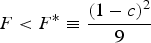 $F \lt F^{\ast} \equiv {\lpar 1 - c\rpar ^2 \over 9}$
. In addition,
 $\bar{t} \gt t_2^E$
, as long as
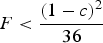
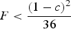 $F \lt {\lpar 1 - c\rpar ^2 \over 36}$
. This fee yields an overall social welfare of
 $SW^{NE}\lpar \bar{t}\rpar = {3\sqrt{F}\left[4 - \lpar 3 + 6d\rpar \sqrt{F} - 4c \right]\over 4}$
, whereas the social welfare from setting an inflexible fee t
E
that attracts entry is
 $SW^{E}\left(t^{E}\right)= {49 - 49 \lpar 2 - c\rpar c \over 50\lpar 1 + 2d\rpar } - F$
.
The following lemma examines the regulator's incentives to set entry-deterring fees when the institutional setting is inflexible. (All proofs are relegated to the appendix.)
Lemma 1
Under an inflexible policy regime, the social welfare from an entry-deterring fee
 $\bar{t}\comma \; SW^{NE}\left(\bar{t}\right)$
, exceeds that from setting a fee t
E
that attracts entry, SW
E
(t
E
), if and only if F > F
Inflex
(d). Furthermore, cutoff F
Inflex
(d) satisfies F
Inflex
(d) < π
ent
E
(t
E
), where
 $$F^{Inflex}\lpar d\rpar \equiv {1310 + 8d\lpar 557 + 459d\rpar - 60\sqrt{2}\lpar 1 - c\rpar ^2 G - M\lpar 2 - c\rpar c \over 25\lpar 5 + 28d + 36d^2\rpar }$$
and
 $G\equiv \left[\lpar 1 + 2d\rpar ^3 \lpar 205 + 18d\rpar \right]^{1 \over 2}$
and
 $M\equiv 2\lpar 1 + 2d\rpar \lpar 655 + 918d\rpar $
. In addition,
 $\bar{t} \gt 0$
since cutoff F* lies above π
ent
E
(t
2
E
) for all parameter values.
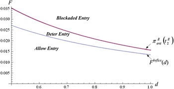
Figure 2 represents cutoff F
Inflex
(d) for the case where
 $c = {1\over 4}$
. Intuitively, when entry costs are higher than F
Inflex
(d), entry can be deterred by setting a low fee
 $\bar{t}$
, thereby incurring a small welfare loss. For (F, d)-pairs below F
Inflex
(d), in contrast, entry deterrence becomes more difficult since it requires a high emission fee
 $ \bar{t}$
, thereby producing a large welfare loss. Hence, allowing entry is socially optimal.Footnote
13
,
Footnote
14
Entry patterns under an inflexible regime

5. Welfare comparisons across regimes
We can now evaluate the welfare properties of the two policy regimes. As described above, emission fees can be used as an entry-deterrence device when the regulator operates under an inflexible policy.
Let us introduce additional notation. Let F
Flex
(d) represent the entry cost that solves
 $SW^{NE}\lpar \bar{t}\rpar =SW^{E} \left(t_{1}\comma \; t_{2}^{E}\right)$
. That is, the regulator is indifferent between selecting a stringent fee,
 $\bar{t}$
, that deters entry under an inflexible regime and setting equilibrium fees that attract entry, (t
1,t
2
E
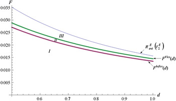
), under a flexible policy. Figure 3 depicts such a cutoff, which lies above cutoff F
Inflex
(d) under all feasible values of d.Footnote
15
The following proposition summarizes the policy regime that yields the largest social welfare under different parameter conditions in the subgame-perfect equilibrium of the game. For presentation purposes, let region I represent entry costs where F < F
Inflex
(d) (see figure 3), region II the case in which F
Inflex
(d) < F < F
Flex
(d), and region III denote the case where F
Flex
(d) < F < π
ent
E
(t
2
E
).
Proposition 1
In equilibrium, policy regimes satisfy:
-
(1) In regions I and II, a flexible policy that attracts entry yields the largest welfare; and
-
(2) In region III, an inflexible policy
 $\bar{t}$
that deters entry yields the largest welfare.

Welfare comparison between flexible and inflexible regimes

The ranking of policy regimes can therefore be divided into three regions. When entry costs are sufficiently low, F < F
Inflex
(d), flexible regimes are socially optimal, since they yield a larger social welfare than an inflexible policy. This case is graphically represented in region I of figure 3. Intuitively, entry can only be deterred by selecting a relatively stringent fee
 $\bar{t}$
, which reduces the incumbent's monopoly output during both periods, thus significantly decreasing consumer and producer surplus. As a consequence, the welfare loss from setting
 $\bar{t}$
offsets its associated savings in entry costs and environmental pollution, and a flexible environmental policy is welfare superior. A similar argument holds when entry costs are moderately low, F
Inflex
(d) < F < F
Flex
(d) in region II, where flexible policies also yield a larger welfare.Footnote
16
When entry costs are relatively high, however, social welfare can be maximized by deterring entry. Specifically, in region III, entry can be deterred by imposing a relatively low
 $\bar{t}$
, thereby incurring small welfare losses from reducing the incumbent's monopoly output. In this setting, an inflexible policy yields a larger social welfare.Footnote
17
Summarizing, our results suggest that inflexible environmental policies are particularly beneficial in industries with high entry costs (such as cement, oil and gas, etc.), but flexible regimes are beneficial when entry costs are low.Footnote
18
Finally, the region under which entry deterrence becomes socially optimal (region III) shrinks in firms' marginal costs. In particular, an increase in c produces a downward shift in the entrant's duopoly profits, π ent E (t 2 E ), reducing the distance π ent E (t 2 E ) − F Flex (d). Intuitively, when the entrant is more inefficient, its profits upon entry decrease, making him less attracted to the market, and hence the regulator's task of deterring entry becomes less necessary.
6. Can entry-deterring policies be opposed by the incumbent?
From a policy perspective, stringent environmental policies that deter entry are commonly regarded as a policy instrument incumbent firms can favor. The next proposition shows, however, that in certain contexts the incumbent might actually lobby against the introduction of such entry-deterring regulation.
Proposition 2
The incumbent's profits are larger when the regulator sets an entry-deterring fee
 $\bar{t}$
than under any other policy regime if and only if F > F
Profits
(d), where
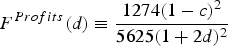 $F^{Profits}\lpar d\rpar \equiv {1274\lpar 1-c\rpar ^2 \over 5625\lpar 1 + 2d\rpar ^2}$
. Hence, the incumbent and regulator's preferences over the entry-deterring fee
 $\bar{t}$
are misaligned when
 $F^{Flex}\lpar d\rpar \lt F\leq F^{Profits}\lpar d\rpar $
, but aligned when
 $F^{Profits} \lpar d\rpar \lt F\leq \pi_{ent}^E \left(t_{2}^E \right)$
.
In particular, fee
 $\bar{t}$
helps the incumbent maintain her monopoly power. However, given the stringency of
 $\bar{t}$
, this fee significantly reduces her output and profits during both periods. As a consequence, the incumbent prefers that the regulator deters entry only when fee
 $\bar{t}$
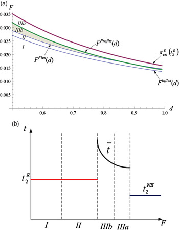
, and thus the profit loss that she must bear, is relatively small. This specifically occurs when entry is easy to deter, i.e., entry costs are relatively high. In order to illustrate this result, figure 4 superimposes cutoff F
Profits
(d) on figure 3, thus breaking the entry-deterring region III into two sub-areas: region IIIa, in which the regulator and incumbent's preferences are aligned, and region IIIb (shaded area), where preferences are misaligned. In particular, deterring entry is sequentially rational for the regulator in IIIb, but such a practice imposes a significant profit loss on the incumbent, thereby diminishing her overall profits. In summary, when entry costs are sufficiently high, both the regulator and the incumbent are willing to bear the cost of a stringent environmental policy in order to deter entry. In contrast, when entry costs are relatively low (in the shaded area), entry deterrence becomes costly, implying that the incumbent prefers entry rather than bearing the large cost of the strict fee
 $\bar{t}$
that avoids entry (as depicted in figure 4b), whereas the regulator still finds entry deterrence socially optimal.Footnote
19
In particular, figure 4 illustrates the duopoly fee t
2
E
that the regulator would set in regions I and II of figure 4, where he allows entry; the entry-deterring fee
 $\bar{t}$
that he would set under region III; and the emission fee that the regulator sets in the context of blockaded entry, i.e., when
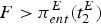 $F \gt \pi_{ent}^{E}\lpar t_2^E\rpar $
.
(a) Profits in the entry-deterring equilibrium and (b) Emission fees in each region

7. Conclusions
Our paper examines under which conditions governments may have incentives to set relatively stringent environmental policies in order to maximize social welfare. We show that entry deterrence becomes socially optimal when its associated welfare loss, due to setting a stringent fee across time which induces an inefficient production level, is smaller than its welfare gain, which arises from the savings in entry costs and environmental pollution. Otherwise, a flexible regime that attracts entry is welfare superior. In addition, we demonstrate that the incentives of the social planner and incumbent are not necessarily aligned regarding entry deterrence. In particular, under certain conditions the regulator finds it socially optimal to choose an inflexible policy that deters entry whereas the incumbent would actually prefer a flexible policy that attracts entry.
The paper assumes that the entrant observes the incumbent's cost before deciding whether to join the industry. In different settings, however, the entrant might not have access to this information, thereby using the incumbent's production decision and the regulator's environmental policy as signals in order to infer the incumbent's costs. While in a context without environmental regulation the incumbent can strategically use output decisions to convey or conceal information from the potential entrant, the introduction of emission fees could distort the incumbent's entry-deterring behavior. In addition, we consider a single incumbent, which could be modified to allow for multiple incumbents, as in Gilbert and Vives (Reference Gilbert and Vives1986). Unlike their work, however, free-riding incentives are absent in our model since the incumbents' output choices do not condition entry decisions. Another extension to our model could consider that firms select not only their output but that, for a given abatement technology, they also choose their abatement level. Finally, our paper can be extended to the analysis of non-polluting goods, such as solar panels. In this case, the regulator would not impose taxes but rather provide subsidies in order to induce firms to produce the socially optimal output.
Appendix 1: Flexible policy regime
No entry. Given a second-period fee t 2, under no entry the incumbent solves
 $$\mathop{\max}\limits_{x_{inc}} \lpar 1 - x_{inc}\rpar x_{inc} - \lpar c + t_2\rpar x_{inc}$$
which yields an output function
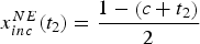 $x_{inc}^{NE} \lpar t_{2}\rpar = {1 - \left(c + t_2 \right)\over 2}$
. The social planner seeks to induce an output level that maximizes social welfare,
 $$\mathop{\max}\limits_{x_{inc}} CS\lpar x_{inc}\rpar + PS\lpar x_{inc}\rpar + T_{2}^{NE} - d\times \lpar x_{inc}\rpar ^2\comma \;$$
where
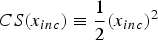 $CS\lpar x_{inc}\rpar \equiv {1 \over 2}\lpar x_{inc}\rpar ^2$
, PS(x
inc
) ≡ (1 − x
inc
)x
inc
− (c + t
2) x
inc
denote consumer and producer surplus, respectively, and T
2
NE
≡ t 2 x
inc
represents tax revenue under no entry. Taking first-order conditions, we obtain the socially optimal output
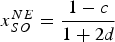 $x_{SO}^{NE} = {1 - c \over 1 + 2d}$
. Hence, the emission fee t
2 that induces the monopolist to produce x
SO
NE
is that solving the equation
 $${1 - \lpar c + t_2\rpar \over 2} = {1 - c \over 1 + 2d}\comma \;$$
i.e.,
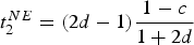 $t_{2}^{NE} = \lpar 2d - 1\rpar {1 - c \over 1 + 2d}$
, or more compactly t
2
NE
= (2d − 1)x
SO
NE
, which is positive for all
 $d\gt {1 \over 2}$
. (A similar fee, t
1 = (2d − 1)q
SO
, is implemented in the first period, since the incumbent is the unique firm operating in the market, where x
SO
NE
= q
SO
NE
.)
Entry. In the case of entry, the incumbent (entrant) solves
 $$\eqalign{&\mathop{\max}\limits_{x_{inc}} \lpar 1-x_{inc}-x_{ent}\rpar x_{inc}- \lpar c+t_{2}\rpar x_{inc}\quad \hbox{and}\cr &\mathop{\max}\limits_{x_{ent}} \lpar 1-x_{ent}-x_{inc}\rpar x_{ent} - \lpar c + t_{2}\rpar x_{ent} - F}$$
respectively, yielding an output function
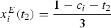 $x_i^E \lpar t_2\rpar = {1 - c_i - t_2 \over 3}$
for any firm i = {inc,ent}. The social planner seeks to induce an output level X that maximizes
 $$\mathop{\max}\limits_{X} CS\lpar X\rpar + PS\lpar X\rpar + T_{2} - d \times X^2$$
where X ≡ x
inc
+ x
ent
,
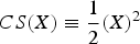 $CS\lpar X\rpar \equiv {1 \over 2} \lpar X\rpar ^2$
, PS(X) ≡ (1 − X)X − (c + t
2) X − F, and T
2 ≡ t
2
X. Note that the producer surplus PS(X) considers the incumbent's marginal costs. This is due to the fact that, in order to allocate the production decision of the socially optimal output, the social planner equally splits it between incumbent and entrant, since both firms are equally efficient. Taking first-order conditions, we obtain the aggregate socially optimal output
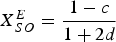 $X_{SO}^{E} = {1 - c \over 1+2d}$
, which coincides with x
SO
NE
. Finally, in order to find fee t
2
E
and individual output levels x
inc,SO
E
and x
ent,SO
E
, the social planner must simultaneously solve
 $$x_{inc\comma SO}^{E}+x_{ent\comma SO}^{E} = {1 - c \over 1 + 2d}$$
(the sum of incumbent's and entrant's output coincides with the socially optimal output X SO ) and
 $$x_{inc}^{E}\lpar t_{2}\rpar = {1-c-t_{2} \over 3}\comma \; \quad \hbox{and}$$
 $$x_{ent}^{E}\lpar t_{2}\rpar = {1-c-t_{2} \over 3}.$$
Simultaneously solving equations A.1–A.3, yields the emission fee
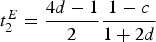 $t_{2}^{E}= {4d-1 \over 2} {1 - c \over 1 + 2d}$
, or
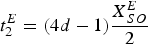 $t_{2}^{E} = \lpar 4d - 1\rpar {X_{SO}^{E} \over 2}$
, which is strictly positive if
 $d\gt {1 \over 4}$
, a condition that holds given that
 $d \gt {1 \over 2}$
by assumption. Substituting fee t
2
E
into the output function x
i
E
(t
2) yields
 $x_{inc}^{E}\lpar t_{2}^{E}\rpar = x_{ent}^{E}\lpar t_2^E\rpar = {1 \over 2} {1 - c \over 1 + 2d} = {X_{SO}^E \over 2}$
, i.e., the socially optimal output is equally split among the incumbent and the entrant. ■
Entry-deterring fee. The entry-deterring fee
 $\bar{t}$
that solves π
ent
E
(t) = F, i.e.,
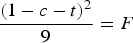 ${\lpar 1 - c - t\rpar ^2 \over 9} = F$
, is
 $\overline{t} = 1 - c - 3 \sqrt{F}$
. Such a fee is hence larger than the equilibrium fee under a flexible policy regime, t
2
E
, as long as
 $c \lt 1 - 2\lpar 1 + 2d\rpar \sqrt{F}$
. This condition can be alternatively expressed as
 $F \lt {\lpar 1 - c\rpar ^2 \over 4\lpar 1 + 2d\rpar ^2}$
. In addition, given that
 $d\in \left[{1 \over 2}\comma \; 1 \right]$
, this cutoff starts at
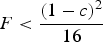 $F \lt {\lpar 1 - c\rpar ^2 \over 16}$
when
 $d = {1 \over 2}$
, and decreases in d, reaching
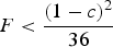 $F \lt {\lpar 1 - c\rpar ^2 \over 36}$
when d = 1. Therefore, for
 $\bar{t} \gt t_2^E$
to hold under all admissible values of d, we need that entry costs satisfy
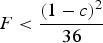 $F \lt {\lpar 1 - c\rpar ^2 \over 36}$
. ■
Appendix 2: Inflexible policy regime
Let us first separately find the deadweight loss from setting a constant fee t in the first period, DWL 1, and in the second period, DWL 2. The first-period deadweight loss from setting an inefficient fee t is
 $$DWL_1 \lpar t\rpar \equiv \vint_{q\lpar t\rpar }^{q_{SO}} \left[SMB^{NE}\lpar q\rpar - MD^{NE} \lpar q\rpar \right]dq$$
where socially optimal output q
SO
is
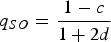 $q_{SO} = {1 - c \over 1 + 2d}$
, and the monopolist output function is
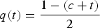 $q\lpar t\rpar = {1 - \lpar c + t\rpar \over 2}$
. In addition, SMB
NE
(q) = (1 − q) − c, whereas MD
NE
(q) = 2dq. Integrating, we obtain
 $$DWL_{1}\lpar t\rpar = {\left[\lpar 2d - 1\rpar c + 1 + t - 2d\lpar 1 - t\rpar \right]^2 \over 8A}$$
where A≡ 1 + 2d. In the second-period game, the deadweight loss from the inflexible fee t is
 $$DWL_2 \lpar t\rpar \equiv \vint_{X^E \lpar t\rpar }^{X_{SO}^E} \left[SMB^E \lpar X\rpar - MD^E \lpar X\rpar \right]dX\comma \;$$
where socially optimal output is still
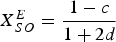 $X_{SO}^{E} = {1 - c \over 1 + 2d}$
, and X
E
(t) = x
inc
E
(t) + x
ent
E
(t), where
 $x_{inc}^{E}\lpar t\rpar = x_{ent}^{E}\lpar t\rpar = {1 - \lpar c + t\rpar \over 3}$
represent the output function that each firm uses to respond to a given fee t under duopoly. Furthermore, SMB
E
(X) = (1 − X) − c, whereas MD
NE
(X) = 2dX. Integrating, we obtain
 $$DWL_{2}\lpar t\rpar = {\left[\lpar 4d - 1\rpar c + 2 + 2t - 4d\lpar 1 - t\rpar - 1\right]^2 \over 18A}.$$
The regulator can construct the sum DWL
1(t) + DWL
2(t) (note that both DWL
1(t) and DWL
2(t) are strictly positive) and take first-order conditions with respect to t, obtaining fee
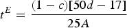 $t^{E} = {\lpar 1 - c\rpar \lsqb 50d-17\rsqb \over 25A}$
. In addition, the emission fee t
E
yields the minimum of the objective function DWL
1(t) + DWL
2(t) since such a function is convex in t, i.e.,
 ${\partial^2 \lsqb DWL_1 \lpar t\rpar + DWL_2 \lpar t\rpar \rsqb \over \partial t^2} = {25A \over 36} \gt 0$
for all parameter values.
Finally, fee t
E
can be expressed as a linear combination of the equilibrium fees under a flexible policy, t
1 and t
2
E
, by solving t
E
= αt
1 + (1 − α)t
2
E
, where parameter α describes the relative weight on first-period taxes. Solving for parameter α yields
 $\alpha = {9 \over 25}$
. Hence,
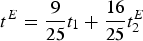 $t^{E} = {9 \over 25} t_{1}+ {16 \over 25} t_2^E$
, and thus t
1 < t
E
< t
2
E
. From our analysis of the flexible policy, we know that fee t
2
E
is positive and induces positive output levels from both firms in the industry. Therefore, a lower fee t
E
in the inflexible policy regime must also induce positive production levels from both incumbent and entrant. ■
Proof of Lemma 1: Under an inflexible policy regime, the social welfare from setting a constant entry-deterring fee
 $\bar{t}=1 - c - 3 \sqrt{F}$
is
 $$SW^{NE} \lpar \bar{t}\rpar = {3\sqrt{F}\left[4 - \lpar 3 + 6d\rpar \sqrt{F} - 4c\right]\over 4}$$
where the incumbent produces according to the monopoly output function
 $q\lpar t\rpar = {1 - c \over 2}$
during both periods. If, in contrast, the regulator selects a constant fee t
E
, entry ensues, yielding an overall social welfare of
 $$SW^{E}\lpar t^{E}\rpar = {49 - 49\lpar 2 - c\rpar c \over 50\lpar 1 + 2d\rpar } - F$$
Hence, the regulator prefers to deter entry, i.e.,
 $SW^{NE}\lpar \bar{t}\rpar \gt SW^E \lpar t^E\rpar $
, if F > F
Inflex
(d), where
 $$F^{Inflex}\lpar d\rpar \equiv {1310 + 8d\lpar 557 + 459d\rpar - 60\sqrt{2}\lpar 1 - c\rpar ^2 G - M\lpar 2 - c\rpar c \over 25\lpar 5 + 28d + 36d^2\rpar }$$
and
 $G\equiv \lsqb \lpar 1 + 2d\rpar ^3 \lpar 205 + 18d\rpar \rsqb ^{1 \over 2}$
and M ≡ 2(1 + 2d)(655 + 918d). First, note that cutoff F
Inflex
(d) is decreasing in d for all costs c ∈ (0, 1). Second, cutoff F
Inflex
(d) lies below
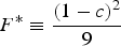 $F^{\ast }\equiv {\lpar 1 - c\rpar ^2 \over 9}$
for all admissible values of d, i.e.,
 $d\in \left({1 \over 2}\comma \; 1\right)$
. In particular, the highest point of cutoff F
Inflex
(d),
 $F^{Inflex} \left({1 \over 2}\right)$
, is
 $${557 - 30\lpar 1 - c\rpar ^2 \sqrt{214} - 557\lpar 2 - c\rpar c \over 2450}$$
which is lower than
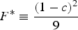 $F^{\ast}\equiv {\lpar 1 - c\rpar ^2 \over 9}$
, which is constant in d, for all costs c ∈ (0, 1). Third, cutoff F
Inflex
(d) also lies below the entrant's duopoly profits under the flexible fee t
2
E
, π
ent
E
(t
2
E
). Specifically,
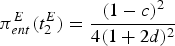 $\pi_{ent}^{E}\lpar t_{2}^{E}\rpar = {\lpar 1 - c\rpar ^2 \over 4\lpar 1 + 2d\rpar ^2}$
is decreasing in d, reaching its highest value at
 $d = {1 \over 2}$
,
 ${\lpar 1 - c\rpar ^2 \over 16}$
, which lies above
 $F^{Inflex}\left({1 \over 2}\right)$
; and reaches its lowest value at d = 1,
 ${\lpar 1 - c\rpar ^2 \over 36}$
, which also lies above F
Inflex
(1). Fourth, note that the entrant's duopoly profits under the inflexible fee t
E
,
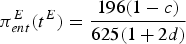 $\pi_{ent}^E \lpar t^E\rpar = {196\lpar 1 - c\rpar \over 625\lpar 1 + 2d\rpar }$
, satisfy π
ent
E
(t
E
) > π
ent
E
(t
2
E
) since t
E
< t
2
E
, i.e., t
E
is less stringent than t
2
E
. Therefore, if F
Inflex
(d) satisfies F
Inflex
(d) < π
ent
E
(t
2
E
), then
 $$F^{Inflex}\lpar d\rpar \lt \pi_{ent}^E \lpar t_2^E\rpar \lt \pi_{ent}^E \lpar t^E\rpar .$$
Finally, note that profits π
ent
E
(t
E
) lie below cutoff F*. Indeed, π
ent
E
(t
E
) reaches its highest point at
 $d = {1 \over 2}$
,
 ${49\lpar 1 - c\rpar ^2 \over 625}$
, which is lower than cutoff F*. Since F* is constant in d, then F* > π
ent
E
(t
E
) under all parameter values. □
Proof of Proposition 1: Let us compare the social welfare that arises in the case that the regulator operates under a flexible regime or under an inflexible regime and, if so, whether he allows or deters entry. Entry ensues as long as the constant fee % t does not exceed
 $\bar{t}$
. In particular, overall social welfare from flexible emission fees t
1 and t
2
E
is
 $SW^{E}\left(t_{1}\comma \; t_{2}^{E}\right)= {1 - \lpar 2 - c\rpar c \over 1 + 2d} - F$
, that of a constant fee t
E
that allows entry is
 $SW^{E}\lpar t^{E}\rpar = {49 - 4 9\lpar 2 - c\rpar c \over 50\lpar 1 + 2d\rpar } - F$
, and that of an entry-deterring fee
 $\bar{t}$
is
 $SW^{NE}\lpar \bar{t}\rpar = {3\sqrt{F} \left[4 - \lpar 3 + 6d\rpar \sqrt{F} - 4c\right]\over 4}$
. It is straightforward to show that
 $SW^E \left(t_1 \comma \; t_2^E \right)\gt SW^{NE} \lpar \bar{t}\rpar $
when F < F
Flex
(d), where
 $$F^{Flex}\lpar d\rpar \equiv {\psi - 48\lpar 1 - c\rpar ^2 \lpar 1 + 2d\rpar ^{3/2} - R \over \lpar 5 + 28d + 36d^2\rpar ^2}$$
and ψ ≡ 52 + 16d(11 + 9d) and R ≡ 4(1 + 2d)(13 + 18d)(2 − c)c. In addition,
 $SW^{NE}\lpar \bar{t}\rpar \gt SW^E \left(t^{H\comma E} \right)$
when F > F
Inflex
(d), as described in Lemma 1, and F
Inflex
(d) < F
Flex
(d). This implies that when F < F
Inflex
(d), social welfare satisfies
 $SW^E \left(t_1\comma \; t_2^E \right)\gt SW^E \left(t^E \right)\gt SW^{NE} \lpar \bar{t}\rpar $
, and a flexible policy regime yields the largest social welfare; when F
Inflex
(d) < F < F
Flex
(d), social welfare satisfies
 $SW^E \left(t_1\comma \; t_2^E \right)\gt SW^{NE} \lpar \bar{t}\rpar \gt SW^E \left(t^E \right)$
, and a flexible policy still entails the largest social welfare; when F
Flex
(d) < F < π
ent
E
(t
2
E
), social welfare satisfies
 $SW^{NE}\lpar \bar{t}\rpar \gt SW^E \left(t_1\comma \; t_2^E \right)\gt SW^E \left(t^E \right)$
, and an inflexible fee
 $\bar{t}$
that deters entry generates the largest welfare; and when F > π
ent
E
(t
2
E
), entry is blockaded and both policy regimes yield the same social welfare. □
Proof of Proposition 2: The incumbent's profits when the regulator sets an entry-deterring fee
 $\bar{t}=1-c-3\sqrt{F}$
are
 ${9F \over 4}$
during both the first and second period, where the incumbent produces according to the monopoly output function
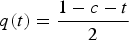 $q\lpar t\rpar = {1 - c - t \over 2}$
during both periods, yielding an overall profit of
 ${18F \over 4}$
. If the regulator chooses a flexible policy regime, with equilibrium fees t
1 and t
2
E
for the first and second period, respectively, the incumbent's profits become
 ${\lpar 1 - c\rpar ^2 \over \lpar 1 + 2d\rpar ^2}$
in the first period and
 ${\lpar 1 - c\rpar ^2 \over 4\lpar 1 + 2d\rpar ^2}$
in the second period (after entry ensues). Hence, overall profits are
 ${5\lpar 1 - c\rpar ^2 \over 4\lpar 1 + 2d\rpar ^2}$
. Therefore, profits under the entry-deterring fee
 $\bar{t}$
are larger than under the flexible fees (t
1, t
2
E
) for all F > F
Profits,Flex
(d) where
 $F^{Profits\comma Flex}\lpar d\rpar \equiv {5\lpar 1 - c\rpar ^2 \over 18\lpar 1 + 2d\rpar ^2}$
. If the regulator selects an inflexible policy regime, with equilibrium fee t
E
, the incumbent's profits become
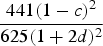 ${441\lpar 1 - c\rpar ^2 \over 625\lpar 1 + 2d\rpar ^2}$
in the first period and
 ${196\lpar 1 - c\rpar ^2 \over 625\lpar 1 + 2d\rpar ^2}$
in the second period (after entry ensues). Hence, overall profits are
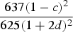 ${637\lpar 1 - c\rpar ^2 \over 625\lpar 1 + 2d\rpar ^2}$
. Therefore, profits under the entry-deterring fee
 $\bar{t}$
are larger than under the inflexible fee t
E
for all F > F
Profits,Inflex
(d) where
 $F^{Profits\comma Inflex}\lpar d\rpar \equiv {1274\lpar 1 - c\rpar ^2 \over 5625\lpar 1 + 2d\rpar ^2}$
. In addition, note that cutoff F
Profits,Inflex
(d) > F
Profits,Flex
(d), since the difference
 $$F^{Profits\comma Inflex}\lpar d\rpar - F^{Profits\comma Flex}\lpar d\rpar = {98\lpar 1 - c\rpar ^2 \over 625\lpar 1 + 2d\rpar ^2}$$
is positive under all parameter values. Furthermore, π ent E (t E ) > F Profits,Inflex (d) since the difference
 $$\pi_{ent}^{E}\lpar t^{E}\rpar - F^{Profits\comma Inflex}\lpar d\rpar = {98\lpar 1-c\rpar ^2 \over 1125\lpar 1 + 2d\rpar ^2}$$
is positive under all parameter values. Therefore, π
ent
E
(t
E
) > F
Profits,Inflex
(d) > F
Profits,Flex
(d). Hence, the region of parameter values under which the regulator prefers to practice entry deterrence but the incumbent does not occurs when F ≤ F
Profits,Inflex
(d). Otherwise, both agents prefer the entry-deterring fee
 $\bar{t}$
. Therefore, only cutoff F
Profits,Inflex
(d) is binding, and we denote F
Profits,Inflex
(d) as F
Profits
(d). □