





1. Introduction
The mission of the Juno spacecraft around Jupiter in 2016 renewed the interest of the fluid physics community for vortex crystals, as it revealed spectacular vortex structures at the poles of the gaseous planet (Adriani et al. Reference Adriani2018). Vortex crystals are peculiar point vortex configurations that emerge in inviscid two-dimensional fluid flows, where identical vortices place themselves in regular positions, forming a kind of rigid body that rotates at a well-defined angular velocity depending on the intensity of the vortices and on the distance between them (Aref et al. Reference Aref, Newton, Stremler, Tokieda and Vainchtein2002). In the past decades, these structures were observed in various laboratory flows with different materials and scales: superfluid helium (Yarmchuk et al. Reference Yarmchuk, Gordon and Packard1979), pure electron columns (Fine et al. Reference Fine, Cass, Flynn and Driscoll1995; Schecter et al. Reference Schecter, Dubin, Fine and Driscoll1999; Durkin & Fajans Reference Durkin and Fajans2000a , Reference Durkin and Fajansb ), and rotating disks floating on a liquid (Grzybowski et al. Reference Grzybowski, Stone and Whitesides2000; Grzybowski & Whitesides Reference Grzybowski and Whitesides2002). They can emerge spontaneously from disordered vortex distributions in plane flows at large Reynolds numbers (Fine et al. Reference Fine, Cass, Flynn and Driscoll1995; Jin & Dubin Reference Jin and Dubin2000; Siegelman et al. Reference Siegelman, Young and Ingersoll2022; van Kan et al. Reference van Kan, Favier, Julien and Knobloch2024), as well as in forced two-dimensional turbulence (Jiménez & Guegan Reference Jiménez and Guegan2007; Jiménez Reference Jiménez2020). These studies showed a wide variety of vortex crystals, as vortices can either place themselves at the tips of a rotating polygon (with or without an additional vortex at the centre of this polygon), or form more space-filling structures composed of embedded polygons.
The transport of inertial particles in these flows is a topic of interest, as particles are very sensitive to the distribution of vorticity. Throughout the paper, it will be assumed that the suspension is dilute and that the dispersed phase does not affect the fluid flow. When particles are heavier than the fluid, they are known to flee vortex cores because of centrifugal effects. However, when multiple vortices interact, particles can accumulate in various well-defined zones near vortices (Vilela & Motter Reference Vilela and Motter2007; Angilella Reference Angilella, Vilela and Motter2010; Nizkaya et al. Reference Nizkaya, Angilella and Bues2010; Ravichandran et al. Reference Ravichandran, Perlekar and Govindarajan2014; Zhao et al. Reference Zhao, Zuo and Qian2025). The simplest case is the pair of identical point vortices, which rotate around each other until vortex merger takes place. Heavy particles released in this flow can be trapped by two attracting points rotating with the vortex pair (Angilella Reference Angilella, Vilela and Motter2010; Ravichandran et al. Reference Ravichandran, Perlekar and Govindarajan2014). This is due to the fact that in the frame rotating with the pair, anticyclonic recirculation cells are present, and the Coriolis force acts towards the interior of the cell (see also Tanga et al. (Reference Tanga, Babiano, Dubrulle and Provenzale1996) for a description of this phenomenon in accretion disks). Particles with a sufficiently small Stokes number, measuring particle inertia (defined below), will then be driven towards a stable equilibrium point located within the cell.
Anticyclonic cells are also present in the flow due to crystals of vorticity composed of more than two vortices, when the flow is observed in the frame rotating with the crystal. To our knowledge, little has been done to understand the dynamics of particles in such systems. The question of the existence of trapping points within these cells is therefore of interest and has been discussed by Ravichandran et al. (Reference Ravichandran, Deepu and Govindarajan2017). These authors focused on the case where the crystal is composed of
 $N$
identical vortices placed at the tips of a polygon – i.e. regularly placed on the circumscribed circle of the polygon – and could show numerically that attracting points exist for all
 $N \le 7$
. They also calculated numerically the critical Stokes number below which trapping happens. The nature of trapping points (hyperbolic or degenerate) has been investigated recently (Angilella Reference Angilella2024). Particles with a sufficiently small Stokes number were observed to converge towards
 $N$
external hyperbolic trapping points located outside the circumscribed circle. In addition, an unexpected ‘cage effect’ was also observed, where particles attracted towards the degenerate fixed point at the origin slowly converged towards the centre of the polygon. At long times, particles therefore form a mass crystal, i.e. a rigid body, composed of
 $N+1$
points fixed in the frame of the vortex crystal. In these analyses, the flow had no vortex at the centre of the polygon. This configuration has been shown to be stable for
 $N \le 7$
(Mertz Reference Mertz1978; Kurakin & Yudovich Reference Kurakin and Yudovich2002). It is characterised by
 $N+1$
anticyclonic cells:
 $N$
cells with a centre located outside the circumscribed circle, plus one cell around the centre of the crystal.
The present work is devoted to the case where the polygon formed by the vortex crystal has a vortex located at its centre. Indeed, geophysical observations, like laboratory experiments, have shown that this stable configuration is frequent (Durkin & Fajans Reference Durkin and Fajans2000b ; Adriani et al. Reference Adriani2018). Its stability, in the case of point vortices, has been shown theoretically (Mertz Reference Mertz1978). Clearly, the cage effect mentioned above, and the structure of the particle crystal, must be significantly affected by the presence of the central vortex. This transport phenomenon will be studied in two steps. As mentioned above, in the limit of small Stokes numbers, particles are known to possess equilibrium points in the vicinity of the centre of anticyclonic recirculation cells (Angilella Reference Angilella2024). We will therefore study the number and position of such cells as a first step (§ 2). Then the motion of inertial particles in these cells, and the stability of their equilibrium positions, will be investigated (§ 3). In addition, it will be shown that an attracting streamline exists inside the crystal: this one-dimensional attractor will be characterised in § 4. The effects of viscosity on the flow and particle dynamics will be considered in § 5 in various configurations of interest, with or without a central vortex. We summarise our results and conclude in § 6.
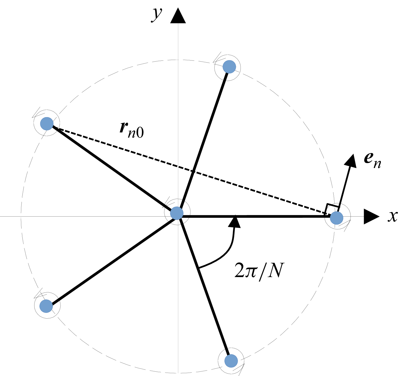
Sketch of vortices placed on the tips of a polygon.

Figure 1. Long description
A sketch of vortices placed on the tips of a polygon. The diagram shows a central point with several blue dots positioned at equal distances around it, forming a regular polygon. Each blue dot represents a vortex. Lines connect the central point to each vortex, indicating their positions relative to the center. The angle between adjacent vortices is labeled as 2π/N, where N is the number of vortices. The radius from the center to any vortex is labeled as r_n0. An arrow labeled e_n points radially outward from one of the vortices, indicating the direction perpendicular to the line connecting the center to the vortex. The diagram illustrates the concept of vortex crystals, where identical vortices arrange themselves in regular positions, forming a rigid body that rotates at a well-defined angular velocity.
2. Anticyclonic cells and particle trapping in vortex crystals
2.1. Inviscid flow structure
We consider the two-dimensional flow of an inviscid and incompressible fluid, composed of
 $N$
identical point vortices with strength
 $\varGamma \gt 0$
, initially located at
 $\boldsymbol x_n = a (\cos (n 2\pi /N), \sin (n 2\pi /N))$
, with
 $n=0,\ldots,N-1$
, in the Cartesian axes attached to the laboratory frame. In addition, a central vortex with strength
 $\varGamma _c$
is located at
 $\boldsymbol x = \boldsymbol 0$
. The velocity induced on vortex
 $n=0$
by all other vortices is
 \begin{equation} \boldsymbol V_0 = \frac {\varGamma }{2\pi } \sum _{n\not = 0} \frac {\boldsymbol e_n}{r_{n0}} + \frac {\varGamma _c}{2\pi a} \boldsymbol e_y, \end{equation}
where
 $\boldsymbol e_n$
is the direct unit vector perpendicular to
 $\boldsymbol x_0 - \boldsymbol x_n$
, and
 $r_{n0}=|\boldsymbol x_0 - \boldsymbol x_n|=2 a \sin (n \pi /N)$
, and
 $\boldsymbol e_y$
is the unit vector along the
 $y$
axis (figure 1). One can check that
 $\boldsymbol V_0 = a \varOmega _0 \, \boldsymbol e_y$
, where
 \begin{equation} \varOmega _0 = (N-1)\frac {\varGamma }{4\pi a^2} + \frac {\varGamma _c}{2\pi a^2}. \end{equation}
By symmetry, all vortices rotate at the same speed
 $\varOmega _0$
, which is the angular velocity of the crystal.
Throughout the paper, relative velocity, relative streamfunction and relative streamlines will refer to these kinematic quantities observed in the reference frame of the vortex crystal, also referred to as ‘the rotating frame’. In this frame, vortices are fixed, the flow is steady, and its streamfunction reads
 \begin{equation} \psi = \frac {1}{2}\varOmega _0\, |\boldsymbol x|^2 - \frac {\varGamma }{4 \pi } \sum _n \ln \big(|\boldsymbol x - \boldsymbol x_n|^2\big) - \frac {\varGamma _c}{4 \pi } \ln \big(|\boldsymbol x|^2\big). \end{equation}
The first term in (2.3) is the streamfunction of a solid body rotating at speed
 $-\varOmega _0$
with respect to the crystal; the second term corresponds to the potential flow due to the satellite vortices, and the latter is the central vortex. The flow in the rotating frame is rotational, with a uniform vorticity
 $-\Delta \psi = -2 \varOmega _0$
. In the remainder of the paper, dimensional quantities are non-dimensionalised using
 $a$
(the radius of the circumscribed circle of the polygon) and
 $\varOmega _0$
(the angular velocity of the crystal with respect to the laboratory frame). Also, we introduce the vortex strength ratio
 $\gamma _c = \varGamma _c/\varGamma$
.
2.2. Dynamics of particles and equilibrium points
The non-dimensional equation of motion for isolated heavy inertial particles transported in this steady flow, in the limit of small particle Reynolds number and neglecting gravity, reads
 \begin{equation} \ddot {\boldsymbol X} = \frac {1}{\textit{St}} (\boldsymbol{u}(\boldsymbol X) - \dot {\boldsymbol X} ) + \boldsymbol X - 2 \boldsymbol{e}_z \times \dot {\boldsymbol{X}}, \end{equation}
where
 $\boldsymbol{X}(t)$
is the position of the particle, and
 $\boldsymbol{u} = \boldsymbol{\nabla }\psi \times \boldsymbol{e}_z$
. Added mass and Basset–Boussinesq forces, as well as pressure gradient of the undisturbed flow (including pressure gradient due to inertial forces acting on the fluid), have been neglected in the heavy-particle limit. The second term on the right-hand side of (2.4) is the non-dimensional centrifugal force due the constant rotation of the reference frame, and the last term is the non-dimensional Coriolis force. The Stokes number is
 $St= \varOmega _0 \tau _p$
, where
 $\tau _p$
is the response time of the particles:
 $\tau _p = m_p/(6 \pi \eta r_p)$
, where
 $\eta$
is the dynamic viscosity of the fluid, and
 $m_p$
and
 $r_p$
denote the mass and radius of the particle. Equilibrium positions of inertial particles are points where drag is balanced by the centrifugal force, and satisfy
 \begin{equation} \boldsymbol \varPhi (\boldsymbol X,\textit{St}) \equiv \boldsymbol{u}(\boldsymbol X) + St\, \boldsymbol X = {\boldsymbol 0} . \end{equation}
The critical Stokes number below which (2.5) admits solutions
 $\boldsymbol X_{eq}$
could be obtained analytically in the cases
 $N=2$
and
 $N=3$
(Angilella Reference Angilella, Vilela and Motter2010, Reference Angilella2024), and numerically for larger
 $N$
(Ravichandran et al. Reference Ravichandran, Perlekar and Govindarajan2014, Reference Ravichandran, Deepu and Govindarajan2017). In the limit
 $St \to 0$
, however, some general results can be obtained for all
 $N$
. Indeed, if the fluid flow has a stagnation point at some position
 $\boldsymbol X_{eq}^0$
, and if the gradient of
 $\boldsymbol{u}$
at
 $\boldsymbol X_{eq}^0$
is invertible, then the implicit functions theorem implies that there exists a continuously differentiable function
 $\boldsymbol X_{eq}(St)$
, defined for sufficiently small
 $St$
, and satisfying
 $\boldsymbol \varPhi (\boldsymbol X_{eq}(St),St)=\boldsymbol 0$
and
 $\boldsymbol X_{eq}(0) = \boldsymbol X_{eq}^0$
. Particles with a sufficiently small Stokes number will then have an equilibrium position in the vicinity of the fluid stagnation point. Let
 $\mu$
denote an eigenvalue of the fluid stagnation point. The characteristic polynomial of the fluid gradient matrix at
 $\boldsymbol X_{eq}^0$
reads (see Appendix A)
 \begin{equation} \mu ^2 = \left (\frac {\partial u}{\partial x} \right )^2 + \left (\frac {\partial u}{\partial y} \right )^2 - 2 \frac {\partial u}{\partial y} \equiv I(\boldsymbol X_{eq}^0), \end{equation}
where we made use of incompressibility and of irrotationality of the flow in the laboratory frame.
To study the nature of the equilibrium position of inertial particles, we rewrite their motion equation (2.4) as a dynamical system with four degrees of freedom for
 $\boldsymbol Y = (x,y,\dot x,\dot y)^{\rm T}$
. The system takes the form
 $\dot {\boldsymbol Y} = \boldsymbol F(\boldsymbol Y)$
. Let
 $\lambda _1,\ldots ,\lambda _4$
denote the eigenvalues of
 $\boldsymbol{\nabla }\!\boldsymbol F$
at
 $\boldsymbol X_{eq}(St)$
(this matrix is given in Appendix A). These eigenvalues are
 \begin{eqnarray} \lambda _{1,3} &=&\frac {1}{2\, \textit{St}}\left ( -1+ (1-4\, \textit{St}^2 \pm 4\, \textit{St}\, \sqrt {I})^{1/2}\right )\!, \end{eqnarray}
 \begin{eqnarray} \lambda _{2,4} &=& - \frac {1}{2\, \textit{St}}\left ( 1+ (1-4\, \textit{St}^2 \pm 4\, \textit{St}\, \sqrt {I})^{1/2}\right )\!, \end{eqnarray}
where
 $I=I(\boldsymbol X_{eq}(St))$
. On expanding
 $I$
in the limit of small Stokes numbers, i.e.
 $I=I_0 + St\, I_1 + St^2\, I_2 + \cdots$
, with
 ${I_0}=I(\boldsymbol X_{eq}^0)$
, we get
 \begin{align} \lambda _{1,3} &= \pm \sqrt {I_0} +\left (-1-I_0 \pm \frac {I_1}{2\sqrt {I_0}}\right ) \textit{St} + O\big(\textit{St}^2 \big), \\[-12pt]\nonumber \end{align}
 \begin{align} \lambda _{2,4} &= - \frac {1}{\textit{St}} \mp \sqrt {I_0} + \left (1+I_0 \mp \frac {I_1}{2\sqrt {I_0}}\right ) \textit{St} + O\big(\textit{St}^2 \big) . \end{align}
These eigenvalues give crucial information about the behaviour of particles in the vicinity of the fluid equilibrium position. If
 $I_0 \gt 0$
, then the fluid stagnation point is a hyperbolic saddle (with eigenvalues
 $\mu = \pm \sqrt I_0$
), and (2.9)–(2.10) show that the particle equilibrium point is also a hyperbolic point with four real non-zero eigenvalues, two of them being positive. It is therefore unstable.
If
 $I_0 \lt 0$
, then the fluid stagnation point is an elliptic centre point (with eigenvalues
 $\mu = \pm {\rm i}\,\sqrt {|I_0|}$
). Equations (2.9)–(2.10) show that the particle equilibrium point is still hyperbolic, i.e. with complex eigenvalues with non-zero real parts. These real parts can be readily calculated, and read
 \begin{align} \text{Re}(\lambda _{1}) &= \text{Re}(\lambda _{3}) = -\big(1+\mu ^2 \big) \textit{St} + O\big(\textit{St}^2 \big), \\[-12pt]\nonumber \end{align}
 \begin{align} \text{Re}(\lambda _{2}) &= \text{Re}(\lambda _{4}) = - \frac {1}{\textit{St}} + \big(1+\mu ^2 \big) \textit{St} + O\big(\textit{St}^2 \big). \end{align}
Equations (2.11)–(2.12) show that if
 $\mu ^2 \lt 0$
and
 $\mu ^2 \gt -1$
, then the equilibrium point
 $\boldsymbol X_{eq}(St)$
is asymptotically stable and attracts particles released in its basin of attraction, in the limit
 $St \to 0$
.
The determination of elliptic fluid stagnation points and the calculation of
 $\mu ^2$
is therefore a quick way to detect possible trapping points of inertial particles in the flow. This is the method adopted in the present work and presented in the following paragraphs for particles in vortex crystals.
2.3. Anticyclonic cells and trapping in the vortex crystal
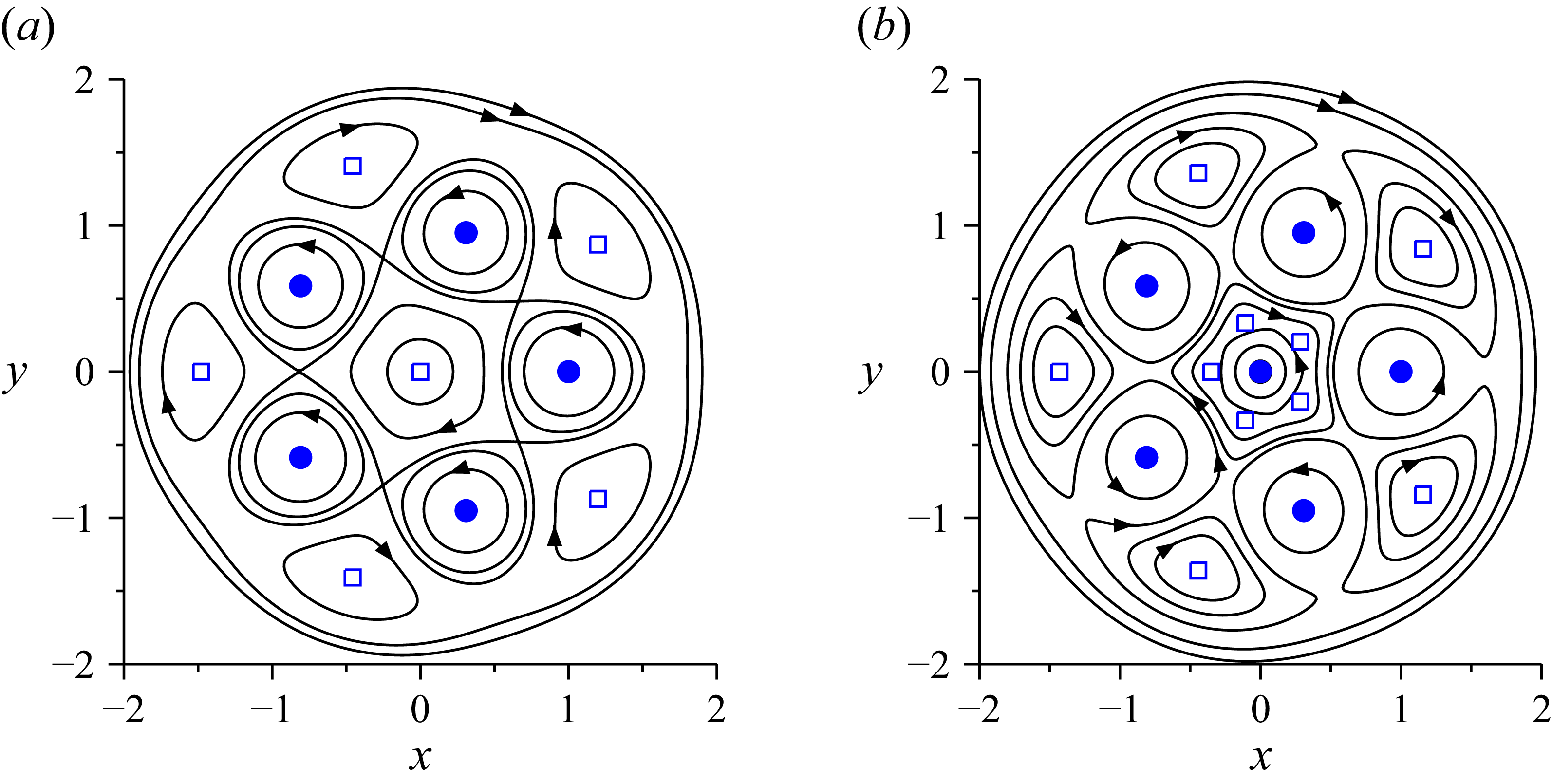
The inspection of the relative streamlines
 $\psi = \text{constant}$
in the case
 $\gamma _c = 0$
shows that the relative flow has a large anticyclonic cell around an elliptic stagnation point located along the axis
 $\theta = \pi /N\ [\text{mod} \ 2\pi /N]$
(see figure 2(a) in the case
 $N=5$
). In the case
 $\gamma _c \gt 0$
, new stagnation points appear along the very same axes. Indeed, one can check that the velocity components
 $u=\partial \psi /\partial y$
and
 $v= -\partial \psi /\partial x$
, calculated along the axis
 $\theta = \pi /N$
, read
 \begin{eqnarray} u &=& f_N(r) \, P_N(r,\gamma _c), \end{eqnarray}
 \begin{eqnarray} v &=& g_N(r) \, P_N(r,\gamma _c), \end{eqnarray}
where
 $f_N(r)$
and
 $g_N(r)$
are non-zero functions, and
 $P_N(\gamma _c,r)$
is a polynomial function of
 $r$
given in Appendix B. The system
 $(u,v)=(0,0)$
is therefore equivalent to
 \begin{equation} P_N(r,\gamma _c) = 0. \end{equation}
Relative streamlines of the flow created by
 $N=5$
vortices with identical strengths
 $\varGamma$
placed on a pentagon. Blue disks indicate the positions of vortices, and squares are elliptic stagnation points at the centre of anticyclonic cells. (a) No central vortex,
 $N+1= 6$
anticyclonic cells are present. (b) A vortex with strength
 $\varGamma _c = \varGamma /4$
has been added at the centre,
 $2 N = 10$
anticyclonic cells are present.

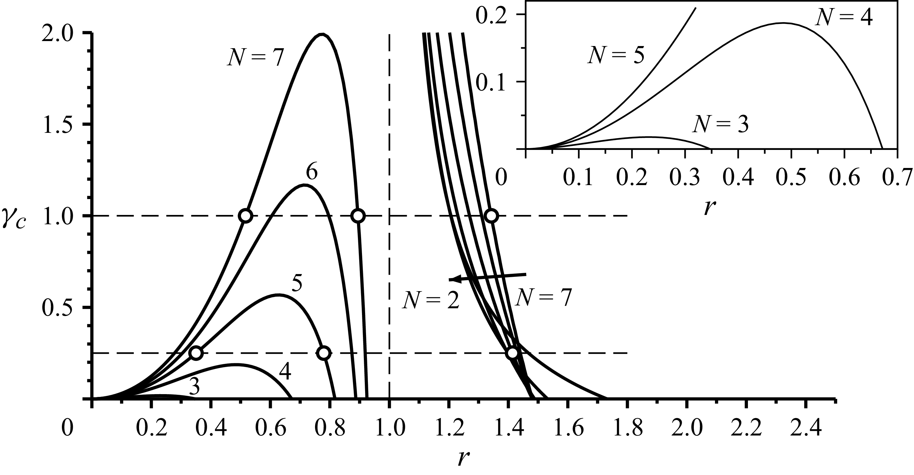
Lines
 $P_N(r,\gamma _c)=0$
, for various values of
 $N$
, indicating the existence of fluid stagnation points along the axis
 $\theta =\pi /N$
. The inset is a zoom of the same graph. The axis
 $\gamma _c=0$
corresponds to the case without central vortex, where
 $N+1$
elliptic stagnation points exist (one at
 $r=0$
, plus
 $N$
external points at
 $r \gt 1$
). When
 $\gamma _c \gt 0$
, equation
 $P_N(r,\gamma _c)=0$
can have three solutions
 $r \gt 0$
for
 $3 \le N \le 7$
, corresponding to
 $3N$
stagnation points,
 $2N$
of which are elliptic points. When
 $\gamma _c$
is above some critical value, internal points vanish.

Figure 3 shows the lines
 $P_N = 0$
in the
 $(r,\gamma _c)$
plane, for various values of
 $N$
. We observe that for
 $\gamma _c = 0$
and
 $3 \le N \le 7$
, only two stagnation points exist along the axis
 $\theta = \pi /N$
, one at
 $r=0$
, and one at
 $ r \gt 0$
. Therefore,
 $N+1$
stagnation points exist in the
 $(x,y)$
plane (one at the centre, plus
 $N$
external points at
 $r \gt 1$
). The stagnation point at
 $r=0$
is a saddle point when
 $N=2$
, and an elliptic point at the centre of an anticyclonic cell when
 $3 \le N \le 7$
(Angilella Reference Angilella2024). When
 $\gamma _c \gt 0$
and
 $N \ge 3$
, (2.15) can have up to three solutions
 $r \gt 0$
, corresponding to
 $3N$
stagnation points in the
 $(x,y)$
plane. The three roots of
 $P_5(r,1/4)$
and
 $P_7(r,1)$
are marked with white circles in figure 3, and are denoted
 $r_1 \lt r_2 \lt r_3$
in the following. Using a numerical solver to determine
 $r_i$
for
 $N=5$
and
 $7$
, we can determine
 $\mu ^2$
at the fluid stagnation points
 $(r_i \cos (\pi /N),r_i \sin (\pi /N))$
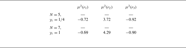
. The result is given in table 1.
Squared eigenvalues of the fluid stagnation points
 $(r_i,\theta =\pi /N)$
identified on figure 3 (circles), for
 $(N,\gamma _c) = (5,1/4)$
and
 $(N,\gamma _c) = (7,1)$
.

Table 1. Long description
A table comparing squared eigenvalues of fluid stagnation points for different values of N and gamma_c. The table has 2 rows and 4 columns. The columns are labeled as N, gamma_c, mu_squared(r1), mu_squared(r2), and mu_squared(r3). Row 1: N = 5, gamma_c = 1/4, mu_squared(r1) = -, mu_squared(r2) = -0.72, mu_squared(r3) = 3.72, mu_squared(r4) = -0.92. Row 2: N = 7, gamma_c = 1, mu_squared(r1) = -, mu_squared(r2) = -0.69, mu_squared(r3) = 4.29, mu_squared(r4) = -0.90.
We therefore conclude that attracting points exist for
 $(N,\gamma _c) = (5,1/4)$
and
 $(N,\gamma _c) = (7,1)$
in the vicinity of
 $(r=r_1,\theta =\pi /N)$
and
 $(r=r_3,\theta =\pi /N)$
, for inertial particles with a sufficiently small Stokes number. In contrast, the point
 $(r=r_2,\theta =\pi /N)$
is a saddle stagnation point in both cases, and no particle trapping point is expected to exist in its vicinity under the current hypotheses. Since the same conclusions hold for
 $\theta =n\pi /N$
,
 $n=1,\ldots,N-1$
, we conclude that
 $2N$
particle trapping points exist in these flows. Half of these
 $2N$
points are located inside the crystal (
 $r \lt 1$
), and half of them are located outside (
 $r \gt 1$
). We also note from figure 3 that when
 $\gamma _c$
is above some critical value that can be readily determined (see table 2), the internal points vanish. In contrast, the external stagnation points are robust and persist for all
 $\gamma _c$
.
Critical value of the central vortex strength ratio
 $\gamma _c$
below which internal anticyclonic cells exist.

Table 2. Long description
A table with two columns and seven rows. The first column is labeled N and the second column is labeled gamma_c^max. The values in the table are as follows: Row 1: N, 2; gamma_c^max, 0.0178. Row 2: N, 3; gamma_c^max, 0.187. Row 3: N, 4; gamma_c^max, 0.568. Row 4: N, 5; gamma_c^max, 1.168. Row 5: N, 6; gamma_c^max, 1.992.
3. Transport and capture of clouds of particles
The analysis presented in the previous section shows that particles must be trapped in anticyclonic cells, provided that their Stokes number is sufficiently small. To verify this, we have solved numerically the transport equation of
 $10^4$
inertial particles in the laboratory frame, together with the inviscid transport equation of vortices under their mutual influence, in the cases
 $(N,\gamma _c) = (5,1/4)$
and
 $(N,\gamma _c) = (7,1)$
. Figure 4(a) shows the cloud of particles (red points) after 20 turns of the crystal, together with the relative flow streamlines, in the former case. A movie of the evolution is available in the supplementary material at https://doi.org/10.1017/jfm.2026.11991. We observe that particles accumulate in 10 zones, in the vicinity of 5 external points (
 $r\gt 1$
) and 5 internal points (
 $r\lt 1$
), as expected. These correspond to the attracting points predicted by the linear analysis of the previous section. For longer times, one would see particles converging towards these points, and the red patches of particles would become much smaller. Similar conclusions hold for simulations in the case
 $(N,\gamma _c) = (7,1)$
(figure 5
a).
Figures 4 and 5 also suggest that some particles converge towards a star-shaped line located in the vicinity of a streamline. Inertial particles at low Stokes numbers have been observed to accumulate near attracting streamlines in various plane flows. This point is discussed in the next section.
(a) Global view of the cloud of particles (red dots) after 20 turns of the crystal (blue disks), together with fluid streamlines (solid lines), in the case of the inviscid computation of vortices forming a pentagon with a central vortex of relative strength
 $\gamma _c=1/4$
. The accumulation of particles is visible near 5 external trapping points and 5 internal trapping points, and in the vicinity of an attracting streamline of equation
 $\psi (x,y)=\psi (x_0^*,0)$
. (b) Plot of the streamfunction variation
 $J(x_0)$
, such that
 $J(x_0^*)=0$
(Haller–Sapsis criterion). (c) The theoretical attracting streamline (black solid line), together with computed particles. The Stokes number is
 $St=0.02$
. See also the movie in the supplementary material.

Figure 4. Long description
Panel A: A scatter plot with fluid streamlines shows the global view of the cloud of particles (red dots) after 20 turns of the crystal (blue disks). The x-axis ranges from -1.5 to 1.5, and the y-axis ranges from -1.5 to 1.5. The accumulation of particles is visible near 5 external trapping points and 5 internal trapping points, and in the vicinity of an attracting streamline. Panel B: A line graph plots the streamfunction variation J(x0) against x0. The x-axis ranges from 0.40 to 0.50, and the y-axis ranges from -2.5 to 1.0. The plot shows a decreasing trend. Panel C: A scatter plot with a theoretical attracting streamline (black solid line) shows computed particles (red dots). The x-axis ranges from -0.2 to 0.4, and the y-axis ranges from 0 to 0.6. The Stokes number is 0.01.
Counterpart of figure 4, with
 $N=7$
and
 $\gamma _c=1$
.

4. Asymptotic identification of the attracting streamline
A necessary condition for the determination of such attracting streamlines has been proposed by Sapsis & Haller (Reference Sapsis and Haller2010). It consists of setting to zero the rate of change of the volume enclosed by the attractor, leading to
 \begin{equation} \int \dot {\boldsymbol{X}} \boldsymbol{\cdot }\boldsymbol{n} \, {\rm d}s = 0, \end{equation}
where the integral is taken over the attracting line,
 ${\rm d}s$
denotes the elementary arc length, and
 $\boldsymbol{n}$
is a unit vector perpendicular to the attracting line. This condition is particularly useful if one makes use of the classical perturbation of (2.4) in the limit of small inertia:
 \begin{equation} \dot {\boldsymbol{X}} = \boldsymbol{u} + \textit{St} \left ( -\boldsymbol{\nabla }\boldsymbol{u} \boldsymbol{\cdot }\boldsymbol{u} + \boldsymbol X - 2 \boldsymbol e_z \times \boldsymbol{u} \right )\!. \end{equation}
In addition, we assume that the attracting streamline is of equation
 $\psi (x,y) = \psi (x_0,0)$
, i.e. it crosses the
 $x$
axis at some position
 $(x_0,0)$
. By making use of the fact that
 ${\rm d}s = | u |\, {\rm d}t = | \boldsymbol{\nabla }\psi |\, {\rm d}t$
and
 $\boldsymbol n = \boldsymbol{\nabla }\psi /| \boldsymbol{\nabla }\psi |$
, the criterion can be recast as a temporal integral
 \begin{equation} J(x_0) \equiv \int _0^{T(x_0)} \left ( -\boldsymbol{\nabla }\psi \boldsymbol{\cdot }\boldsymbol{\nabla }\boldsymbol{u} \boldsymbol{\cdot }\boldsymbol{u} + \boldsymbol{\nabla }\psi \boldsymbol{\cdot }\boldsymbol X - 2\, |\boldsymbol{\nabla }\psi |^2 \right ) {\rm d}t = 0, \end{equation}
where
 $T(x_0)$
is the period of fluid points along the streamline
 $\psi = \psi (x_0,0)$
. Note that
 $J(x_0)$
also corresponds to the difference between fluid streamfunctions at two stroboscopic positions of an inertial particle,
 $\boldsymbol X(0)$
and
 $\boldsymbol X(T(x_0))$
.
Figures 4(b) and 5(b) show a computation of
 $J(x_0)$
in the cases
 $N=5$
and
 $7$
. We observe that
 $J$
has simple zeros at
 $x_0^* \approx 0.447$
(
 $N=5$
) and
 $x_0^* \approx 0.629$
(
 $N=7$
). Particles indeed accumulate near the theoretical streamline
 $\psi =\psi (x_0^*,0)$
(black solid line, figures 4(c) and 5(c)). At long times, they form a mass crystal, in that the attractor is fixed in the rotating frame, but this crystal has dimension 1, in contrast to the mass crystal formed in the absence of the central vortex.
The numbers of particles trapped at (a,d) interior and (b,e) exterior fixed points, and (c,f) the attracting streamline in simulations with (a–c)
 $N=5+1$
vortices and (d–f)
 $N=6+1$
vortices. Parameter combinations for which no particles are trapped are coloured white. The critical
 $\gamma _c$
above which the interior fixed points disappear may be read from (a,d) and compared with table 2. The total numbers of particles are
 $5\times 10^4$
and
 $6\times 10^4$
in the two cases (initialised with uniform number density in the region
 $r\leq 3$
); the colour bar is logarithmic, and particle counts smaller than
 $10$
are discarded.

Figure 6. Long description
Panel A: A contour plot shows the number of particles trapped at interior fixed points for simulations with 5 vortices. The x-axis is labeled St^-1 and ranges from 0 to 200. The y-axis is labeled γc and ranges from 0 to 1.2. The color bar ranges from 1 to 813. Panel B: A contour plot shows the number of particles trapped at exterior fixed points for simulations with 5 vortices. The x-axis is labeled St^-1 and ranges from 0 to 200. The y-axis is labeled γc and ranges from 0 to 1.2. The color bar ranges from 1 to 8728. Panel C: A contour plot shows the number of particles trapped along the attracting streamline for simulations with 5 vortices. The x-axis is labeled St^-1 and ranges from 0 to 200. The y-axis is labeled γc and ranges from 0 to 1.2. The color bar ranges from 1 to 3238. Panel D: A contour plot shows the number of particles trapped at interior fixed points for simulations with 6 vortices. The x-axis is labeled St^-1 and ranges from 0 to 200. The y-axis is labeled γc and ranges from 0 to 1.2. The color bar ranges from 1 to 1537. Panel E: A contour plot shows the number of particles trapped at exterior fixed points for simulations with 6 vortices. The x-axis is labeled St^-1 and ranges from 0 to 200. The y-axis is labeled γc and ranges from 0 to 1.2. The color bar ranges from 1 to 8715. Panel F: A contour plot shows the number of particles trapped along the attracting streamline for simulations with 6 vortices. The x-axis is labeled St^-1 and ranges from 0 to 200. The y-axis is labeled γc and ranges from 0 to 1.2. The color bar ranges from 1 to 4431.
4.1. Particle trapping by vortex crystals
In general, the critical values of
 $\gamma _c\gt 0$
for which the attracting streamline disappears and for which the interior or exterior fixed points disappear are different. In figure 6, we show that the combination of
 $\gamma _c$
and
 $St$
determines whether the interior or exterior fixed points of the attracting streamline can trap particles. The irregular boundaries of the regions of parameter space in which indefinite trapping can occur belie the complex flow field in the vicinity of a vortex crystal.
We note that the attractor can be multi-pronged in the case where
 $\gamma _c \lt 0$
(i.e. when the central vortex has circulation of the opposite sense to the other vortices). However, at the magnitudes
 $|\gamma _c|$
for which the attractor is seen to split into two or more attractors, the vortex crystal is unstable in viscous simulations, and we do not discuss this case further.
5. Effect of viscosity
The potential flows used in the previous sections correspond to an idealised inviscid fluid where vorticity is localised into regions of null volume. Also, the corresponding velocity fields are steady (in the rotating frame) and persist for infinite times. These two conditions are no longer true when viscosity is present: under the effect of viscous diffusion, vortex cores will grow, and vortex merger will eventually occur. However, all previous analyses concerning vortex pairs have shown that attractors exist temporarily in the presence of viscosity, provided that the flow Reynolds number is large (Angilella Reference Angilella, Vilela and Motter2010; Angilella et al. Reference Angilella2014; Ravichandran et al. Reference Ravichandran, Perlekar and Govindarajan2014). Here, using direct numerical simulations of the flow with Lagrangian particle tracking (the numerical method is detailed in Appendix C), we first show that the inviscid theory is robustly reproduced in viscous simulations, in quantitative agreement with the inviscid case. Simulations were performed with
 $1024^2$
grid points and time step
 $\delta t = 0.005$
(non-dimensionalised as in § 2).
In addition, we observe that for
 $\gamma _c = 0$
, different long-term evolutions emerge and have important consequences for the particle concentration field. These various behaviours, which depend on the flow Reynolds number, are described in the following subsections.
5.1. Crystals with a central vortex
Figure 7 shows contours of the vorticity and particle positions for simulations initialised with
 $5+1$
vortices of strengths
 $(\varGamma , \gamma _c)$
. The interior fixed points exist and the crystal of particles is seen for
 $\gamma _c \lt \gamma _c^{\textit{max}} = 0.568$
, as expected (see table 2). A movie of the evolution is available in the supplementary material.
In figure 8, we plot the analogues of figure 7 for
 $N=7$
vortices. As in figure 5, the exterior and interior fixed points and the attracting streamline are seen for
 $\gamma _c = 1$
. The time evolution can be examined in the movie in the supplementary material. However, with a smaller
 $\gamma _c=0.5$
, we see only the attracting streamline and exterior fixed points. The Stokes number
 $St=0.028$
is evidently larger than the critical Stokes number
 $St_c$
for the internal fixed points. We have checked that the internal fixed points are seen briefly for
 $St=0.014$
, and more prominently for
 $St=0.007$
.
(a,c) Iso-contours of vorticity and (b,d) particle locations overlaid with iso-contours of vorticity. (a,b) The interior and exterior fixed points as well as the attracting streamline are seen with
 $N=5$
vortices of strength
 $\varGamma = 1$
, with a central vortex of strength
 $\gamma _c = 0.25$
for particles of Stokes number
 $St = 0.018 \approx 0.02$
. The fixed points also exist for
 $St=0.036$
(not shown). (c,d) For
 $\gamma _c = 0.6 \gt \gamma _c^{\textit{max}}$
(see table 2), only the exterior fixed points are seen for any
 $St$
. The Reynolds number is
 $\textit{Re}=\varGamma / \nu = 2\times 10^4$
(see Appendix C for details). Compare figures 2 and 4, together with the movie in the supplementary material.

Same as figure 7, but with
 $N=7$
vortices, with (a,b) the central vortex strength
 $\gamma _c=1.0$
and Stokes number
 $St=0.032$
(see also the movie in the supplementary material), and (c,d)
 $\gamma _c=0.5$
and
 $St=0.028$
. While the attracting streamline is seen in the latter, the interior fixed points are not.

5.2. Crystals without central vortex
5.2.1. Transition to a circular vortex layer
For Reynolds numbers
 $\textit{Re}=O(10^3)$
, systems of
 $N$
vortices (i.e. for
 $\gamma _c = 0$
) are known to merge azimuthally to lead to an annular generalised Lamb–Oseen (GLO) vortex (e.g. Swaminathan et al. Reference Swaminathan, Ravichandran, Perlekar and Govindarajan2016), which is a circular vortex layer with finite thickness. We observe that inertial particles suspended in such a flow are ‘corralled’ by the annular vortex layer that is the result of the azimuthal merger of the vortices, as shown in figure 9. Since the diffusion of the annular vortex is a relatively slow process, particles remain trapped within the GLO vortex for extended periods. The overall structure of the particle concentration field is close to that obtained for particles released in an inviscid circular vortex sheet with zero thickness. Indeed, for an axisymmetric circular vortex sheet of radius
 $R$
and circulation
 $\varGamma _s$
, vorticity reads
 \begin{equation} \omega (r) = \frac {\varGamma _s}{2\pi R} \, \delta (r - R), \end{equation}
where
 $\delta$
is the Dirac distribution. This flow corresponds to an azimuthal velocity
 $v_\theta (r) = 0$
for
 $r \lt R$
, and
 $v_\theta (r) = \varGamma _s/(2\pi r)$
for
 $r\gt R$
. It can be thought of as a Rankine vortex where the solid core has been replaced by a still-fluid zone, thus creating a velocity discontinuity at
 $r=R$
. If one releases particles in this flow with a uniform initial number density
 $n_0$
over a zone containing the whole disk of radius
 $R$
, then the number density
 $n(r,t)$
at any time can be obtained by making use of the method of characteristics (see Druzhinin Reference Druzhinin1994): for
 $r\lt R$
, we have
 $n(r,t)=n_0$
for all
 $t$
(‘dusty core’ due to corralled particles), and for
 $R \lt r \lt \rho (t) = R (1+\tau _p \varGamma _s^2 t/(\pi ^2 R^4))^{1/4}$
, a void zone, free of particles, develops (
 $n(r,t)=0$
). The radius
 $\rho (t)$
corresponds to the position of particles released at
 $r \to R$
,
 $r\gt R$
, which are centrifuged away by the circular motion at the exterior of the circular sheet. Such particles are not replaced by particles coming from the zone
 $r \lt R$
, as no centrifugation exists in this zone, in contrast with the Rankine vortex. In viscous flow, the vortex sheet evolves in the form (e.g. Swaminathan et al. Reference Swaminathan, Ravichandran, Perlekar and Govindarajan2016)
 \begin{equation} \omega (r,t) = \frac {\varGamma _s}{4\pi \nu t}\,{\rm e}^{-(R^2+r^2)/4\nu t}\, I_0 \left (\frac {\textit{Rr}}{2\nu t} \right )\!, \end{equation}
where
 $I_0$
is the modified Bessel function of the first kind and zeroth order. Both the dusty core and the void zone are visible in our viscous simulations (figure 9). For
 $r \gt \rho (t)$
, a classical centrifugation takes place, and concentration decays with
 $r$
.
(a) Iso-contours of vorticity and (b) particle locations overlaid with iso-contours of vorticity after the merging of a
 $6$
-vortex system, forming an annular vortex layer, at
 $\textit{Re}=666$
without central vortex (
 $\gamma _c=0$
). After merging, some particles remain inside the annular vortex, hence forming a dusty core. As very few particles escape from the dusty core, a void zone expands at the exterior of the annular vortex layer where centrifugation takes place.

Figure 9. Long description
Panel A: A contour plot shows iso-contours of vorticity in a fluid flow. The x-axis ranges from 4 to 9, and the y-axis ranges from 4 to 9. The contours form concentric circles with varying colors indicating different levels of vorticity, transitioning from blue at the outer edges to yellow at the center. Panel B: A scatter plot of particle locations is overlaid with iso-contours of vorticity. The x-axis ranges from 4 to 9, and the y-axis ranges from 4 to 9. The particles are concentrated in a circular region, forming a dusty core, with a void zone expanding outward. The contours are primarily black, indicating the vorticity levels.
(a) Iso-contours of vorticity and (b) particle locations overlaid with iso-contours of vorticity, showing inertial particles of Stokes number
 $St=0.04$
trapped at the exterior fixed points and in the vicinity of the elliptic fixed point at the centroid of the
 $6$
-vortex system with Reynolds number
 $\textit{Re}=10^4$
. The behaviour of the blob of particles near the origin is similar to that seen with an annular vortex (see figure 9), but the distinct vortices lead to a tighter cluster at the origin.

Figure 10. Long description
Panel A: A contour plot displays iso-contours of vorticity. The x-axis ranges from 4 to 9, and the y-axis ranges from 4 to 8. The contours form a hexagonal pattern with high vorticity regions at the vertices and the center of each side. Panel B: A scatter plot overlaid with iso-contours of vorticity shows particle locations. The x-axis ranges from 4 to 8, and the y-axis ranges from 4 to 8. The particles are concentrated in distinct clusters around the vorticity contours, with a tight cluster at the center and smaller clusters at the outer fixed points.
(a,b) Basins of attraction of the particle blob at the origin, plotted at
 $t\approx 20$
, for the
 $6$
-vortex system at (a)
 $\textit{Re}=666$
and (b)
 $\textit{Re}=10^4$
. (c,d) Particle number densities for the
 $6$
-vortex systems from figure 9 at (c)
 $\textit{Re}=666$
and (d)
 $\textit{Re}=10^4$
. The blob is more closely packed in the latter.

(a) Iso-contours of vorticity and (b) particle locations overlaid with iso-contours of vorticity, showing the intermediate
 $4$
-vortex stage that results from the disintegration of a
 $7$
-vortex system with
 $\gamma _c=0$
, and persists for
 $\approx 30$
flow time units. Inertial particles are trapped at the (external) fixed points for the
 $4$
-vortex system. The Reynolds number is
 $\textit{Re}=5\times 10^4$
. Note that the vortices are of unequal strength in the intermediate stage.

Figure 12. Long description
Panel A: A contour plot displays iso-contours of vorticity. The x-axis ranges from 4 to 9, and the y-axis ranges from 4 to 8. The plot shows four distinct vortices with varying strengths, indicated by different contour levels. The vortices are arranged in a symmetric pattern, with some contours forming closed loops around the vortices. Panel B: A scatter plot overlaid with iso-contours of vorticity. The x-axis ranges from 4 to 8, and the y-axis ranges from 4 to 8. The scatter plot shows the locations of inertial particles trapped at the fixed points of the vortex system. The iso-contours of vorticity highlight the structure of the vortices, with four main vortices visible. The vortices are of unequal strength, as indicated by the varying contour levels.
5.2.2. Break-up into a smaller crystal and persistence of trapping
The
 $N$
-vortex system ultimately evolves into a single vortex of positive sign at the origin. For the large Reynolds numbers considered here, the disintegration of the
 $N$
-vortex crystal can, proceeding with pairwise mergers of vortices, lead to the formation of intermediate regimes with
 $M\lt N$
vortices. We observe that such
 $M$
-vortex systems can also trap particles at the attracting fixed points associated with their geometry. In figure 12, we show an example of this behaviour where the
 $7$
-vortex crystal with
 $\gamma _c = 0$
and
 $\textit{Re}=5\times 10^4$
disintegrates and forms a
 $4$
-vortex intermediate stage. This
 $4$
-vortex system captures some of the particles from the elliptical fixed point at the centroid of the
 $7$
-vortex system that are being centrifuged away, and particles are trapped at the fixed points of the (unequal)
 $4$
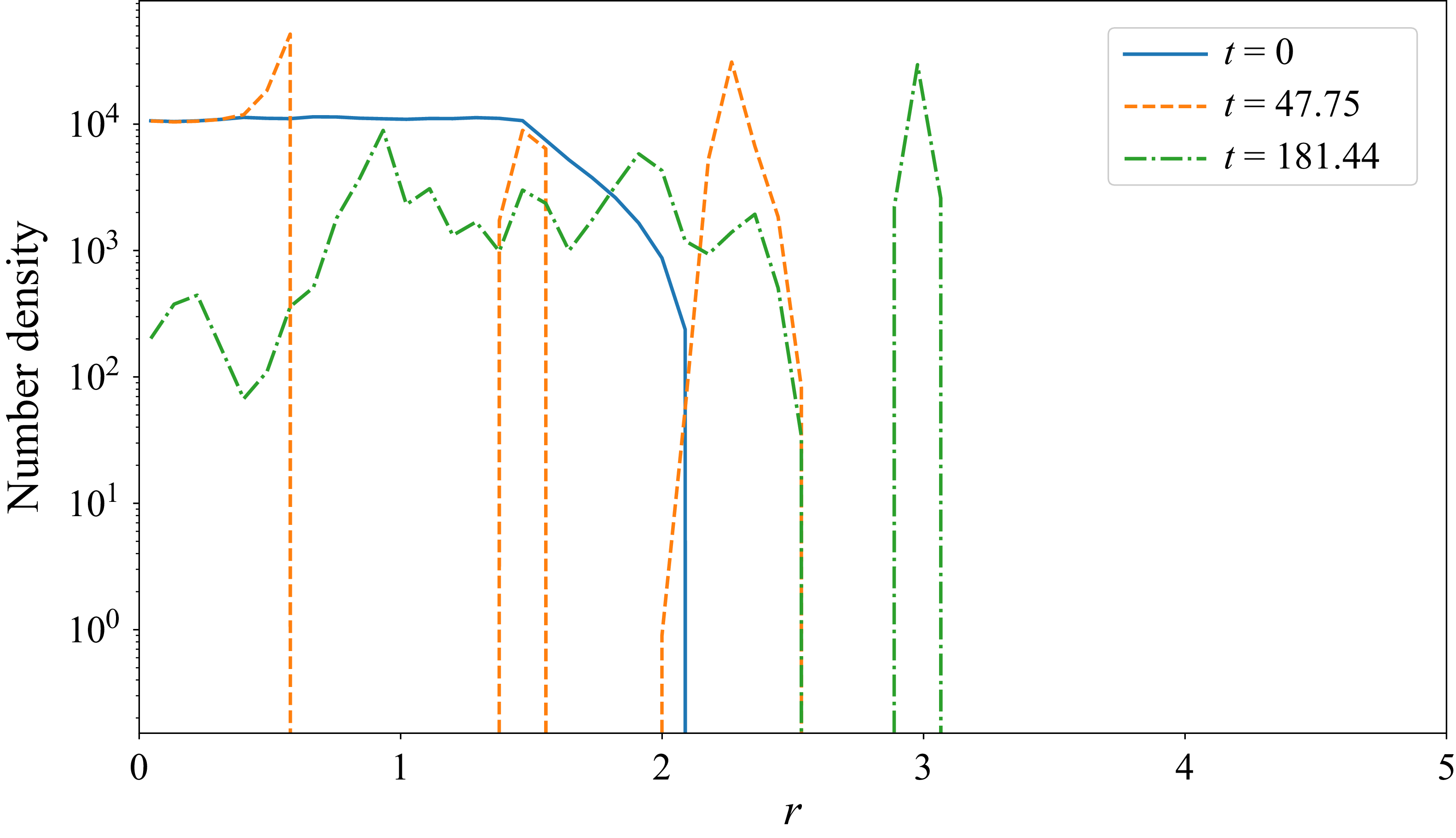
-vortex system for a few dozen flow units. This is seen in the plot of the number density of particles in figure 13, where the initially uniform areal distribution of particle number density is ‘unmixed’, and particles aggregate at the interior and exterior fixed points (
 $t=48$
). Once the
 $7$
vortices have merged into
 $4$
vortices (
 $t=181)$
, particle trapping at the (external) fixed points of the
 $4$
-vortex system is seen as a peak in the number density. Eventually, the smallest of the vortices in the
 $4$
-vortex system is merged into one of the other vortices, quickly followed by the merger of all remaining vortices into a solitary vortex, and the trapped particles are centrifuged out to infinity.
Analogous behaviour is also seen in (
 $N+1$
)-vortex systems (with
 $\gamma _c \gt 0$
), but fewer particles are trapped at the fixed points of the secondary
 $M$
-vortex system since the blob of particles from where these particles are sourced is absent.
The number density of particles per unit area as a function of the radius
 $r$
from the centroid of the vortex crystal for the simulation in figure 12. At
 $t=0$
, the number density is uniform for
 $0\lt r\lt 1.5$
by construction. At
 $t\approx 48$
, we see three spikes. The peak at
 $r\lt 1$
corresponds to increased particle density at the edge of the central blob (see also figure 9), and the peak at
 $r\approx 1.5$
corresponding to the exterior fixed points. The outer ring of particles being centrifuged away is denoted by the peak at
 $r\gt 2$
. At
 $t\approx 181$
, this outermost peak has moved to
 $r\approx 3$
; the peak at
 $r\approx 1$
corresponds to the particles at fixed points of the secondary
 $4$
-vortex system.

6. Discussion and conclusion
We have shown that inertial particles released in an inviscid plane flow characterised by vortices forming a crystal have a variety of attracting positions. In the reference frame rotating with the crystal, these attracting positions are fixed points located in the vicinity of the fluid’s elliptic stagnation points, in the limit where the Stokes number is small. In the presence of a central vortex, an attracting streamline can also appear between the central and satellite vortices, and the position of this streamline could be found by making use of asymptotic techniques (Sapsis & Haller Reference Sapsis and Haller2010).
In the presence of viscosity, these behaviours have been shown to persist until vortex merger takes place. In systems of
 $N+1$
vortices, i.e.
 $N$
annular vortices plus one central vortex, the particles are locally centrifuged away from the vortex at the centroid, but can still be trapped in the vicinity of annular vortices, and form an annular structure topologically similar to the attracting streamline seen in e.g. figures 7 and 8.
After merging, the original crystal no longer exists,
 $\varOmega _0$
is no longer defined, and different behaviours can happen. In the absence of a central vortex, and for large but moderate Reynolds numbers, merging creates a robust annular vortex layer with still fluid (in the laboratory frame) inside a well-defined ring, and a decaying potential vortex flow outside this ring (Swaminathan et al. Reference Swaminathan, Ravichandran, Perlekar and Govindarajan2016). Particles located within the ring are ‘corralled’: they are kept inside this dead zone, and form a dusty core for a large amount of time. Particles located outside this ring are centrifuged away, so that a void zone forms at the exterior of the vortex layer. For larger Reynolds numbers, vortex crystals have been observed to break up into a smaller crystal (e.g. from 7 vortices to a 4-vortex system, figure 12). There, simulations showed that particles could be trapped towards the fixed points of the 4-vortex system.
This work therefore shows that trapping of dust particles in vortex crystals can take different forms and appears in various situations. It can persist even when the vortex crystal evolves under the effect of viscosity. Although vortex merger eventually creates flows with very different structures (annular vortex sheet or smaller crystal), trapping of particles has been shown to persist under different forms.
When particles converge towards accumulation points, one expects inter-particle distances to decrease and particle concentration to grow. The former effect is likely to induce particle–particle interactions, and the latter might alter the fluid flow. Both effects are neglected here since we assumed non-interacting particles and one-way coupling for all times. Also, in the presence of viscosity and particles at semi-dilute concentrations, it was shown that vortex merger could be affected by the dispersed phase (Shuai et al. Reference Shuai, Roy and Kasbaoui2024). The inclusion of these complex effects in our models is a topic of great interest and is left for future studies.
Our results may be applicable to geophysical settings that are characterised by systems of strong vortices. For example, size-dependent preferential clustering of inertial particles in flows dominated by vortices is of interest in hurricanes, and may modify calculations for collisional charge-separation (Black & Hallett Reference Black and Hallett1999). Sapsis & Haller (Reference Sapsis and Haller2009) note that for typical flow speeds seen in hurricanes, inertial effects become significant for particles
 $O(10)$
cm in size (which are likely to be pieces of debris rather than hydrometeors). Attracting points and limit cycles for inertial particles may be explicitly accounted for in such analyses. Studies of idealised eyewalls of hurricanes (Schubert et al. (Reference Schubert, Montgomery, Taft, Guinn, Fulton, Kossin and Edwards1999), see also Swaminathan et al. (Reference Swaminathan, Ravichandran, Perlekar and Govindarajan2016) and references therein) have shown that an instability of the annular vorticity distribution can lead to polygonal vortex formations of the kind studied in detail in previous analyses (Swaminathan et al. Reference Swaminathan, Ravichandran, Perlekar and Govindarajan2016; Angilella Reference Angilella2024) and in the present work. The distribution of hydrometeors (collectively referring to all forms of solid and liquid water particles) in such hurricanes determines the resulting precipitation. Furthermore, collisions between ice particles of different sizes (Dash et al. Reference Dash, Mason and Wettlaufer2001) in such systems lead to the charge separation that is responsible for lightning (see Swaminathan et al. Reference Swaminathan, Ravichandran, Perlekar and Govindarajan2016). In these cases, the mechanisms of (extreme) inertial clustering as the one described here may modify the relevant estimates of collisions and coalescence, leading to precipitation and lightning. In these realistic situations, there might exist velocity components in the vertical direction. Also, gravity can force particles to sink. Both mechanisms can affect the dynamics of particles, so that the pointwise attractors observed here might either be destroyed by these three-dimensional effects, or take the form of more complex attractors (e.g. attracting lines in the direction perpendicular to the main two-dimensional flow). Also, the attracting streamline discussed in § 4 might either vanish or take the form of a multi-dimensional attracting manifold. The detailed analysis of these effects will be considered in the near future.
The accumulation of inertial particles in anticyclones is a well-known phenomenon in astrophysical or geophysical flows (e.g. Barge & Sommeria Reference Barge and Sommeria1995; Tanga et al. Reference Tanga, Babiano, Dubrulle and Provenzale1996; Beron-Vera et al. Reference Beron-Vera, Olascoaga, Haller, Farazmand, Triñanes and Wang2015), where the Coriolis force is induced by the rotation of the planet. The results of the present study show that trapping of objects in anticyclonic zones also appears when the Coriolis force is due to the rotation of a local system of vortices, and is more common than may be realised.
Supplementary movies
Supplementary movies are available at https://doi.org/10.1017/jfm.2026.11991.
Acknowledgements
The authors acknowledge the National Supercomputing Mission (NSM) for providing computing resources through PARAM RUDRA at G02, Ground Floor, IIT Bombay, Powai, Mumbai 400076. PARAM RUDRA is implemented by the Centre for Development of Advanced Computing (C-DAC) and supported by the Ministry of Electronics and Information Technology (MeitY) and the Department of Science and Technology (DST), Government of India.
Funding
S.R. was supported by the IIT Bombay Seed Grant (Grant No. RD/0522-IRCCSH0-020) and the Core Research Grant from the Anusandhan National Research Foundation (ANRF) (Grant No. ANRF/F/1930/2024–2025).
Declaration of interests
The authors report no conflict of interest.
Appendix A. Eigenvalues of fluid and particle equilibrium positions
If
 $\mu$
is an eigenvalue of the fluid gradient matrix, then we have
 \begin{align} (u_{,x} - \mu )(v_{,y}-\mu ) - v_{,x} u_{,y} = 0, \end{align}
where the comma indicates the derivation. We make use of incompressibility, i.e.
 $u_{,x}+v_{,y}=0$
. Also, the flow in the laboratory frame is irrotational, so the relative velocity field
 $(u,v)$
has uniform vorticity
 $-2$
(as times have been set non-dimensional by
 $1/{\varOmega}_0$
), so
 $v_{,x} - u_{,y}=-2$
. This leads to
 \begin{align} (u_{,x} - \mu )(u_{,x} + \mu ) + (u_{,y}-2) u_{,y} = 0, \end{align}
and to (2.6).
The particle dynamics is written as a dynamical system with four degrees of freedom,
 $\dot {\boldsymbol{Y}} = \boldsymbol F(\dot {\boldsymbol{Y}})$
, where
 $\dot {\boldsymbol{Y}}=(x,y,\dot x,\dot y)^{\rm T}$
. The gradient of
 $\boldsymbol F$
at some equilibrium position
 $\boldsymbol X_{eq}(St)$
reads
 \begin{equation} \boldsymbol{\nabla }\!\boldsymbol F = \left ( \begin{array}{cccc} 0 & 0 & 1 & 0 \\[7pt] 0 & 0 & 0 & 1 \\[7pt] u_{,x}/{\textit{St}}+1 & u_{,y}/{\textit{St}} & -{1}/{\textit{St}} & 2 \\[7pt] v_{,x}/{\textit{St}} & v_{,y}/{\textit{St}} + 1 & -2 & -{1}/{\textit{St}} \end{array} \right )\!, \end{equation}
Appendix B. Fluid stagnation points
The system
 $(u,v)=0$
is equivalent to
 $P_N(r,\gamma _c)=0$
, where
 \begin{align} P_2(\gamma _c,r) &= {r}^{4}-3{r}^{2}+2\gamma _c ({r}^{4}-1), \\[-12pt]\nonumber \end{align}
 \begin{align} P_3(\gamma _c,r) &= {r}^{5}-3{r}^{3}+{r}^{2}+\gamma _c ({r}^{5} - {r}^{3}+ {r}^{2}-1), \\[-12pt]\nonumber \end{align}
 \begin{align} P_4(\gamma _c,r) &= 3{r}^{6}-8{r}^{4}+3{r}^{2}+2\gamma _c({r}^{6}- {r}^{4} + {r}^{2}-1), \\[-12pt]\nonumber \end{align}
 \begin{align} P_5(\gamma _c,r) &= 2{r}^{7}-5{r}^{5}+2{r}^{2}+ \gamma _c ({r}^{7}-{r}^{5} + {r}^{2}-1), \\[-12pt]\nonumber \end{align}
 \begin{align} P_6(\gamma _c,r) &= 5{r}^{8}-12{r}^{6}+5{r}^{2}+ 2\gamma _c({r}^{8}-{r}^{6} +{r}^{2}-1). \end{align}
The polynomial
 $P_7(\gamma _c,r)$
has a much longer expression and will not be given here.
Appendix C. Pseudo-spectral solver for viscous simulations
In the laboratory frame, the Navier–Stokes equations,
 \begin{eqnarray} \boldsymbol{\nabla}\boldsymbol{\cdot} u = 0 , \end{eqnarray}
 \begin{eqnarray} \frac {{\rm D}\boldsymbol{u}}{{\rm D}t} = -\boldsymbol{\nabla }\!p + \frac {1}{\textit{Re}}{\nabla} ^2 \boldsymbol{u}, \end{eqnarray}
where
 $\textit{Re} = \varGamma / \nu$
is the Reynolds number, and
 $\nu$
is the kinematic viscosity, are integrated in two spatial dimensions
 $(x,y)$
and time
 $t$
using a pseudo-spectral solver previously used in the same context (e.g. Ravichandran & Govindarajan Reference Ravichandran and Govindarajan2017; Ravichandran & Wettlaufer Reference Ravichandran and Wettlaufer2023). The equations are integrated in time using a third-order low-storage strong-stability-preserving Runge–Kutta method (Gottlieb et al. Reference Gottlieb, Shu and Tadmor2001), modified to use Crank–Nicolson time-stepping for the viscous terms. The nonlinear terms are dealiased by setting Fourier coefficients with
 $|k| \gt 2k_{max}/3$
to zero.
The motion equation of heavy particles submitted to a linear Stokes drag reads
 \begin{equation} \frac {{\rm d}\boldsymbol{v}}{{\rm d}t} = \frac {\boldsymbol{u-v}}{\textit{St}} , \end{equation}
which is effectively (2.4) in an inertial frame. The trajectories of particles are found by integrating (C3) in time with the second-order exponential time-differencing scheme of Cox & Matthews (Reference Cox and Matthews2002). The fluid velocity at the particle location is obtained using bilinear interpolation.
Simulations are initialised with
 $N$
Gaussian vortices of strength
 $\varGamma =1$
and radius
 $r_v = 0.1$
on the vertices of a regular polygon in a doubly periodic box in the region
 $(0,4\pi )\times (0,4\pi )$
, with or without the central vortex of relative strength
 $\gamma _c$
at
 $(2\pi ,2\pi )$
. A total of
 $10^5$
particles are initialised with the local fluid velocity in a region of size
 $3\times 3$
centred at the origin.
The fluid solver has been previously validated in Ravichandran & Wettlaufer (Reference Ravichandran and Wettlaufer2023) (see supplementary material). Here, we provide validation for the method used to integrate the particle equations of motion. In figure 14, we present a snapshot of a simulation with
 $N=2$
vortices, and
 $St=0.16$
. For these parameters, attracting fixed points exist, as seen in Angilella (Reference Angilella, Vilela and Motter2010) and Ravichandran et al. (Reference Ravichandran, Perlekar and Govindarajan2014), and are recovered in the viscous simulations.
Particles of Stokes number
 $St=0.16$
(black dots) aggregate at the two stable fixed points around two vortices at a non-dimensional time
 $t=23.71$
(in units of
 $\varOmega _0^{-1}$
; see text). The Reynolds number is
 $\textit{Re}=10^4$
. (a,b) Results from a simulation with
 $1024^2$
grid points and time step
 $\delta t=0.01$
. (c,d) Results from a simulation with
 $512^2$
grid points and
 $\delta t = 0.01$
. The thin line in (a,c) connects the centres of the vortices. The angle that the thin line makes with the horizontal is displayed on top of each plot. The stable and unstable fixed points from Angilella (Reference Angilella, Vilela and Motter2010) are also shown (blue dots).

Figure 14. Long description
The image contains four contour plots labeled (a), (b), (c), and (d). Each plot shows the aggregation of particles (black dots) around vortex structures. Panel A: A contour plot with grid points and time step. The plot shows the centers of the vortices connected by a thin line, with an angle displayed at the top. Blue dots indicate stable and unstable fixed points. Panel B: A contour plot with a color scale representing vorticity (ω) values ranging from 0 to 2.4. The plot shows particle aggregation around vortices at a non-dimensional time. Panel C: A contour plot with grid points and. The plot shows the centers of the vortices connected by a thin line, with an angle displayed at the top. Blue dots indicate stable and unstable fixed points. Panel D: A contour plot with a color scale representing vorticity (ω) values ranging from 0 to 2.4. The plot shows particle aggregation around vortices at a non-dimensional time.
 N=5
 Γ
 N+1=6
 Γc=Γ/4
 2N=10
 PN(r,γc)=0
 N
 θ=π/N
 γc=0
 N+1
 r=0
 N
 r>1
 γc>0
 PN(r,γc)=0
 r>0
 3≤N≤7
 3N
 2N
 γc
 (ri,θ=π/N)
 (N,γc)=(5,1/4)
 (N,γc)=(7,1)

 γc

 γc=1/4
 ψ(x,y)=ψ(x0∗,0)
 J(x0)
 J(x0∗)=0
 St=0.02

 N=7
 γc=1

 N=5+1
 N=6+1
 γc
 5×10⁴
 6×10⁴
 r≤3
 10

 N=5
 Γ=1
 γc=0.25
 St=0.018≈0.02
 St=0.036
 γc=0.6>γcmax
 St
 Re=Γ/ν=2×104

 N=7
 γc=1.0
 St=0.032
 γc=0.5
 St=0.028

 6
 Re=666
 γc=0

 St=0.04
 6
 Re=104

 t≈20
 6
 Re=666
 Re=104
 6
 Re=666
 Re=104

 4
 7
 γc=0
 ≈30
 4
 Re=5×10⁴
 r
 t=0
 0
 t≈48
 r<1
 r≈1.5
 r>2
 t≈181
 r≈3
 r≈1
 4

 St=0.16
 t=23.71
 Ω0−1
 Re=104
 10242
 δt=0.01
 5122
 δt=0.01


 Open access

