

1. Introduction
This article examines the relationship between political regimes and sovereign credit risk over the long run. The chosen period, 1750–1913, captures key transformations to European political institutions. Study of the process of financial development in Europe is also valuable because countries around the world have implemented its forms of fiscal governance.Footnote 1 An understanding of the European growth experience thus translates into useful lessons for emerging economies today.
Our framework for analysis follows Dincecco (Reference Dincecco2009a) and consists of two core elements. The first comes from North and Weingast (Reference North and Weingast1989). They claim that institutional reforms with the Glorious Revolution of 1688 allowed the English crown to make a credible commitment to responsible debt service.Footnote 2 Since the new constitution gave parliament a regular right to monitor spending decisions, the executive could keep promises to execute fiscal plans in time-consistent ways.Footnote 3 The second part comes from Epstein (Reference Epstein2000). He argues that institutional fragmentation within countries and not fiscal abuse by rulers was the fundamental cause of fiscal distortions prior to the 1800s.Footnote 4 In fragmented polities, there was a close relationship between local tax control and political autonomy. Thus, elites had strong incentives to oppose structural reforms that threatened traditional rights. The result was a classic public goods problem, since each locality wished to free ride on the tax contributions of others. Dincecco (Reference Dincecco2009a) finds that per-capita revenues collected by fragmented sovereignties were low. A lack of resources made it difficult for national governments to repay debts. Centralized from medieval times, England – the example that North and Weingast proffer – was exceptional.Footnote 5
I argue that the political transformations identified by North and Weingast and Epstein were complementary rather than competing elements of sound fiscal policy. By 1913, many European countries had struck an institutional balance that allowed national governments to gather enough in tax revenues while limiting executive discretion over expenditures. To evaluate my hypothesis, I adopt a systematic approach that examines the effects of political reforms on sovereign credit risk both within and across European polities. My investigation thus complements case study texts by Hoffman and Norberg (Reference Hoffman and Norberg1994), Bonney (Reference Bonney1999), Bordo and Cortés-Conde (Reference Bordo and Cortés-Conde2001) and others.Footnote 6
I first construct a new panel data set on government bond yields for 11 European countries. Long yearly series of relevant fiscal data characterize group 1, which includes many of the largest and/or most important players in Europe at the time: England, France, the Netherlands, Prussia, and Spain. The second group (Austria-Hungary, Belgium, Denmark, Italy, Portugal, and Sweden) has shorter data series. I then classify political regimes according to Dincecco (Reference Dincecco2009a). Fiscal centralization was typically the result of French conquest from 1789 to 1815. Limited government generally took place decades after centralization during the 1800s.
The statistical framework that I use is innovative in that it consists of two components not often employed together: regressions on the panel data set and structural break tests. The regressions incorporate a relevant set of control variables (violent conflict, economic growth, and fiscal and monetary policy) to assess the effects of political regimes on sovereign credit risk. For robustness, I include structural break tests that assume no a priori knowledge of major turning points. The statistical inquiry supports the argument that political transformations towards centralized and limited regimes led to significant creditworthiness improvements.
The rest of the paper proceeds as follows. Section 2 examines the relationship between political regimes and creditworthiness. Section 3 describes the data and sample countries. Section 4 examines the data on a case-by-case basis. Section 5 discusses the statistical framework. Section 6 presents the statistical results. Section 7 concludes.
2. Political regimes and sovereign risk
2.1. Historical overview
This section describes the relationship between political arrangements and sovereign credit risk. The classification of political regimes follows Dincecco (Reference Dincecco2009a), who argues that national governments completed the process of fiscal centralization the year that they began to secure revenues by way of a tax system with uniform rates throughout the country. Dincecco claims that limited government emerged the year in which parliament gained the constitutional right to control the national budget on an annual basis. For stability, parliament's power of the purse had to hold for at least two consecutive decades.
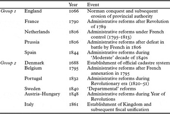
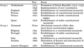
Tables 1 and 2 reproduce Dincecco's dates for fiscal centralization and limited government. The first table indicates that fiscal centralization took place swiftly and permanently throughout much of the Continent from 1789 onwards. The National Assembly transformed the tax system in France by eliminating traditional exemptions and privileges. Napoleon completed this process after his coup in 1799. French conquest of Belgium, the Dutch Republic and several Italian polities led to significant tax reforms. After defeat in battle by France in 1806, Prussia also made major fiscal innovations. The second table indicates that limited government reforms began during the 1830s and 1840s, several decades after centralization. A second wave occurred in the 1860s and 1870s.
Fiscal centralization in Europe

Source: Dincecco (Reference Dincecco2009a).
Notes: The first column lists sample countries by group. Long annual data series over a variety of political regimes characterize group 1, which includes the largest and/or most important players in Europe at the time. Group 2 has shorter data series. The second column displays the year that fiscal centralization was completed. The final column offers brief ‘explanations’ for the dates.
Limited government in Europe

Source: Dincecco (Reference Dincecco2009a).
Notes: The first column lists sample countries by group, which Table 1 describes. The second column displays the year that limited government emerged. The final column offers brief ‘explanations’ for the dates.
Some exceptions bear mention. At one extreme, England had centralized institutions and parliamentary government long before most Continental regimes. At the other, the French failed in their attempts to make administrative changes in Iberia: fiscal centralization in Portugal and Spain did not happen until 1832 and 1844, respectively. Though political risks and instability dominated the peninsula over the 1800s, stable limited regimes were established in Portugal in 1851 and in Spain in 1876.
2.2. Theoretical implications
By establishing parliament's power of the purse, limited government reduced the likelihood of poor spending choices by executives. Ceteris paribus, it should have improved sovereign credit risk, as expressed by a reduction in yield spreads over benchmark British consols, relative to absolutist regimes. The relationship between fiscal centralization and credit risk is less straightforward. On one hand, centralization generated a significant increase in per-capita revenues (see Dincecco Reference Dincecco2009a), which made it easier for crowns to follow sound fiscal policies. Thus, credit risk should have fallen. On the other hand, consolidation of fiscal powers by monarchs may have aggravated problems of executive control. There was always the danger that executives would waste new revenues on ill-advised wars. If so, then credit risk should have increased after centralization.
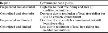
Table 3 summarizes the sovereign credit risk characteristics of the four possible political regimes: fragmented and absolutist, centralized and absolutist, fragmented and limited, and centralized and limited. Note that there was only one example of the fragmented and limited regime among sample countries.Footnote 7 Credit risk under centralized and limited regimes should have been lower than under fragmented and absolutist ones. By eliminating local free riding, fiscal centralization implied an increase in public funds. Similarly, limited government established spending constraints on executives. The combination of greater revenues and parliamentary control should have improved credit risk.
Sovereign credit risk characteristics of political regimes

Sources: See text.
By the same logic, credit risk should have decreased under fragmented and limited regimes in comparison with fragmented and absolutist ones. Theory cannot predict if there was an improvement in credit risk under centralized and absolutist regimes in comparison with fragmented and absolutist ones, since fiscal centralization generated additional funds that executives may have used to repay debts or spent recklessly. However, we may say definitively that credit risk under centralized and limited regimes should have been the lowest of all, since both sorts of fiscal problems had been resolved.
3. Data and sample countries
I assembled a database on long-term government bonds in Europe from 1750 to 1913. Appendix 1 documents the data sources and construction methods for each sample country. Since bond prices often exhibited high volatility, the use of annual data (i.e. one observation per year) increases the likelihood of misrepresenting yield trends. To avoid this possibility, I calculated yearly averages of weekly or monthly data. The yield series came in large part from secondary sources such as the Global Financial Database (GFD), which offered high-frequency data. For accuracy, I compared the GFD series that I computed with annual data from Homer and Sylla (Reference Homer and Sylla1991).
The historical nature of the yield series merits special attention. To begin, demand for sovereign bonds was not integrated or elastic. Governments faced different domestic and international opportunities to market their debts. As Appendix 1 describes, bonds for group 1 countries were typically traded on home exchanges, whereas bonds for group 2 countries were traded on the London Stock Exchange. Prior to 1815, most governments did not offer a public asset comparable to the British consol (i.e. perpetual, dominant, easily negotiable and relatively risk-free), but instead issued a multitude of debt instruments, each subject to different terms and conditions. In such cases, I chose the sovereign bond that best captured long-term yield levels. Appendix 1 provides the details.
The sample was divided into two groups based on data availability and historical importance. Annual published series of nearly a century or more for government bonds as well as for a variety of controls typically existed for the five polities (England, France, the Netherlands, Prussia and Spain) that comprised the first set. Not only were these countries among the largest and/or most powerful players in Western Europe at the time, but for them data were also available over a variety of political regimes.
Shorter published time series existed for the six countries (Austria-Hungary, Belgium, Denmark, Italy, Portugal and Sweden) in the second group. Data for Belgium and Italy only began after they were founded as constitutional monarchies in 1831 and 1861, respectively. Annual series for Austria-Hungary, Portugal, and Sweden did not start until after the establishment of centralized and limited regimes during the 1800s.Footnote 8 Since Denmark did not achieve a stable form of constitutional government by 1913, it functioned as an additional ‘absolutist’ control in the regressions. Though data prior to political transformations were not available for the second set of countries, their inclusion enriched the sample by expanding the range of institutional experiences.
4. Case studies
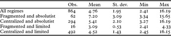
Table 4 displays the summary statistics for the yield panel.Footnote 9 In total, there are 864 observations, 62 for fragmented and absolutist regimes, 294 for centralized and absolutist ones, and 492 for centralized and limited ones; 16 observations characterize the lone fragmented and limited regime. One immediately notices that average yields associated with centralized and absolutist regimes (5.41 percent) and centralized and limited ones (4.52 percent) were low relative to fragmented and absolutist ones (7.20 percent). Average yields for the fragmented and limited regime (3.09 percent) were also much lower.Footnote 10

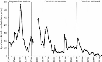
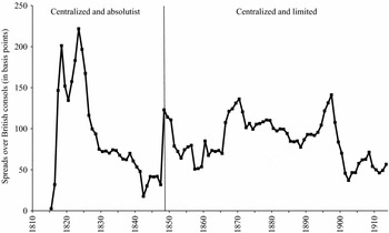
Before moving on to the statistical analysis, it is worthwhile to study France and the Netherlands, two sample polities for which long data series are available. Figure 1, which plots yield spreads between French long-term government bonds and British consols from 1750 to 1913, indicates that yield spreads were typically 200 basis points or more under the fragmented and absolutist regime. The French Revolution (1789–99) led to the establishment of a national tax system with uniform rates. Spreads remained high through the end of the Napoleonic Wars. Unlike the eighteenth century, however, France no longer defaulted on its debts.Footnote 11
Yield spreads, France, 1750–1913

French yield spreads decreased after 1815. The short-lived constitutional ‘July’ regime (1830–47) saw spreads that were less than 50 basis points.Footnote 12 Under the authoritarian regime of Napoleon III (1851–70), however, they doubled to over 100 basis points. Spreads fell steadily after the establishment of a stable centralized and limited regime in 1870. By the start of the 1890s, they neared zero.
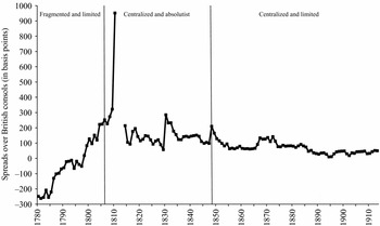
Figure 2 plots yield spreads in basis points between Dutch long-term government bonds and British consols from 1780 to 1913. I followed Dincecco's (Reference Dincecco2009a) classification of the political regime in the Dutch Republic (1572–1795) as fragmented and limited. By investing heavily in government bonds, ruling elites aligned lender and borrower incentives and provided a credible commitment to repay debts. Figure 2 highlights the success of this mechanism. Since the Republic received loans at lower rates of interest than Britain, spreads at the start of the 1780s were negative. Van Zanden and van Riel (Reference Zanden van and Riel van2004), however, argue that widespread fiscal fragmentation hindered the ability of the Republic to raise funds and service debts. Indeed, spreads rose quickly in the years before the French conquered the Netherlands in 1795.Footnote 13
Yield spreads, Netherlands, 1780–1913

The 1815 constitution granted absolutist control to King Willem I, who came to power at the end of the Napoleonic era. Parliamentary budget authority, promulgated at 10-year intervals, was ineffective. Spending heavily on the military, on infrastructure, and on the monarchy itself, Willem was unable to balance the national accounts, though fiscal centralization in 1806 had roughly doubled the size of the Dutch tax base and Europe was politically stable. Dincecco (Reference Dincecco2009b) argues that rapid growth in Dutch deficits from 1815 onwards reflected the reckless policies that Willem pursued. Yield spreads rose with the Belgian Revolt of 1830 and subsequent War of Independence (1830–1833).Footnote 14 In hope of reclaiming Belgium, Willem continued to spend great sums on the military. During the 1830s, Dutch spreads remained around 150 basis points higher than spreads under the constitutional ‘July’ regime in France. When Dutch fiscal troubles finally became public in 1839, parliament vetoed the upcoming decadal budget and Willem abdicated his throne. As parliament's power of the purse increased over the 1840s, spreads fell to 100 basis points. After the Revolutions of 1848, which saw the establishment of a stable centralized and limited regime, spreads typically remained less than 100 basis points through the start of World War I.
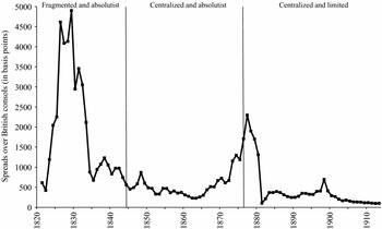
To supplement the French and Dutch cases, it is useful to examine the rest of the data. Figure 3, which plots yield spreads between Spanish long-term government bonds and British consols from 1820 to 1913, indicates that spreads fell by roughly 500 basis points after fiscal centralization in 1844. The establishment of a stable form of limited government in 1876 also led to a sizeable reduction in Spanish spreads.
Yield spreads, Spain, 1821–1913

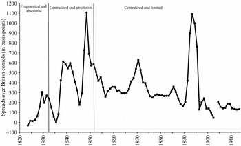
Figure 4, which plots yield spreads between Portuguese long-term government bonds and British consols from 1823 to 1913, indicates that spreads were higher after fiscal centralization in 1832 than beforehand. The period from 1821 to 1851, however, was one of civil war as well as colonial conflict.Footnote 15 Portuguese spreads fell with the establishment of a stable form of limited government in 1851. Moreover, during much of the 1850s and 1860s, spreads in Portugal were typically 100 to 200 basis points lower than those of Spain, its absolutist counterpart on the Iberian Peninsula.
Yield spreads, Portugal, 1823–1913

Figure 5, which plots yield spreads between Prussian long-term government bonds and British consols from 1815 to 1913, indicates that spreads rose in the decades after the establishment of limited government in Prussia in 1848. Infrequent observations from 1842 to 1869, however, may misrepresent Prussian yield trends. Since weekly or monthly data was not available, I used annual data (taken from the last day of trading each year) from Homer and Sylla (Reference Homer and Sylla1991).Footnote 16 Military conflicts also played a role. Though it did not participate in any major wars from 1815 to 1847, Prussia entered four such conflicts from 1848 to 1871.Footnote 17
Yield spreads, Prussia, 1815–1913

Indeed, qualitative accounts suggest a positive relationship between limited government and public finances in Prussia. According to Ferguson (Reference Ferguson1998), Rothschild lenders urged King Frederick William II (1786–97) to implement constitutional reforms as a credible way to improve sovereign credit risk. Tilly (Reference Tilly1966, Reference Tilly1967), moreover, argues that the constitutional reforms of 1848 strengthened the ability of the Prussian parliament to follow sound fiscal policies. Finally, the quantitative analysis by Dincecco (Reference Dincecco2009a) finds that limited government in Prussia led to a significant increase in per-capita tax revenues.Footnote 18
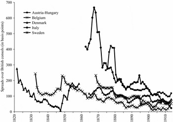
Though the evidence presented so far suggests that political transformations had important effects on sovereign credit risk, it is not definitive. Figure 6, which plots yield spreads for group 2 countries from 1820 to 1913, highlights the importance of controls for factors besides political regime. By the 1870s, for instance, it is difficult to distinguish between deficit ratios associated with the absolutist regime in Denmark and those associated with limited regimes elsewhere. To account for the effects of violent conflict, economic growth, fiscal and monetary policy, and other elements, I now turn to a more rigorous quantitative analysis.
Yield spreads, group 2 countries, 1820–1913

5. Statistical tests
5.1. Panel regressions
Estimations of panel data increase informative content by combining variations across time and country. I followed Beck and Katz (Reference Beck and Katz1995) and employed ordinary least squares with ‘panel-corrected’ standard errors (PCSE), which corrects for contemporaneously correlated errors and panel heteroskedasticity. To control for serial correlation, I included a common AR1 term.Footnote 19
The basic fixed effects specification is:

where Spreadit is the yield spread with British consols in basis points for country i in year t, Xit is a vector of control variables to be described, μi represent country-specific fixed effects, and ɛit is the disturbance term.Footnote 20 I used dummy variables for centralized and absolutist (CA), fragmented and limited (FL), and centralized and limited (CL) regimes relative to fragmented and absolutist ones as a clear and simple method to measure the effect of political arrangements on sovereign credit risk.Footnote 21
Hoffman and Rosenthal (Reference Hoffman, Rosenthal, Drobak and Nye1997) claim that early modern monarchs valued warfare above all else. For the 1800s, Ferguson (Reference Ferguson2006) argues that political events were more important to investors than economic ones since there was a greater amount of regular information available about them. Sussman and Yafeh (Reference Sussman and Yafeh2000, Reference Sussman and Yafeh2006) also find that financial markets responded quickly to wars and civil unrest. One might expect that the total effect of warfare on sovereign credit risk was negative because it decreased tax revenues and increased public expenditures. Over the long run, however, Kindleberger (Reference Kindleberger1984), Tilly (Reference Tilly1990), Hoffman and Norberg (Reference Hoffman and Norberg1994), Epstein (Reference Epstein2000), O'Brien (Reference O'Brien2001), Rosenthal and Wong (Reference Rosenthal and Wong2007) and others argue that military competition fostered financial innovations that allowed sovereigns to reduce credit risk. Whether a country won or lost a conflict also influenced public finances. To evaluate the impact of warfare on yield spreads, I included a dummy variable that identified each year from 1750 to 1913 in which sample countries were engaged in military conflicts in Western or Eastern Europe according to Clodfelter (Reference Clodfelter2002). Appendix 2 documents the details.
Though debt figures would also be useful to measure the effects of warfare on public finances, continuous series were not available prior to the 1870s (see Ferguson Reference Ferguson2006). One unique source of data that exists from the 1700s onwards is budgetary figures as assembled by Dincecco (Reference Dincecco2009b). To scale estimates across time, Ferguson and Schularick (Reference Ferguson and Schularick2006) claim that sophisticated analyses of government finances typically employed public revenues. Cain and Hopkins (Reference Cain and Hopkins1994) also argue that budget deficit-to-revenue ratios were the statistic most preferred by investors to evaluate macroeconomic policies.Footnote 22 In accordance with the ‘gentlemanly capitalists’ of London, I used this variable as a measure of fiscal prudence. Table 5 indicates that the average deficit ratio was 0.19. The lowest deficit ratio was −0.89 for Spain in 1803 and the largest was 2.93 for France in 1790.

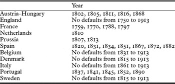
There also exists systematic information for debt default, an extreme reaction to fiscal crisis that caused widespread damage to the financial sector as well as the economy as a whole.Footnote 23 Indeed, early modern executives often resorted to default as a way to handle large debt burdens accumulated during wars.Footnote 24 To measure this effect, I introduced a dummy variable that identified all years of partial or full defaults on publicly held debts from 1750 to 1913 according to Reinhart, Rogoff and Savastano (Reference Reinhart, Rogoff and Savastano2003) and Dincecco (Reference Dincecco2009b). Appendix 2 provides the details.
Since internal conflict caused disruptions that increased sovereign credit risk, we must consider the impact of domestic turmoil as well. To measure this effect, I included a dummy variable that identified all civil wars, coups and revolutions that occurred within sample countries from 1750 to 1913. Appendix 2 describes the details.
One might also suppose that economic growth increased tax bases and enabled sovereign governments to repay debts. Since reliable GDP figures are difficult to come by before 1820, many studies of the late nineteenth century employ measures of foreign trade as approximates of national output (e.g. Mauro, Sussman and Yafeh Reference Mauro, Sussman and Yafeh2002; Obstfeld and Taylor Reference Obstfeld and Taylor2003; Ferguson and Schularick Reference Ferguson and Schularick2006). However, systematic trade deficit and export series from the 1700s onwards were not available. Hohenberg and Lees (Reference Hohenberg and Lees1985), Bairoch (Reference Bairoch1988) and Acemoglu, Johnson and Robinson (Reference Acemoglu, Johnson and Robinson2002, Reference Acemoglu, Johnson and Robinson2005) argue that there was a close relationship between urbanization rates and income growth. To proxy for per-capita GDP, I constructed a yearly variable that calculated urban populations as fractions of total populations for each country. Appendix 2 describes the details.Footnote 25 Controls for national income also help account for different rates of technological innovation and adoption across countries (see Mokyr Reference Mokyr and Castronono1998, Reference Mokyr1999). Table 5 indicates that on average urban populations comprised 17 percent of total populations. The lowest urbanization rates were 4 percent for Prussia during the second half of the 1700s and the largest were over 40 percent for the Netherlands at the start of the 1900s.
Bordo and Rockoff (Reference Bordo and Rockoff1996) and Obstfeld and Taylor (Reference Obstfeld and Taylor2003) claim that adherence to the classic gold standard was a valuable signal of financial integrity. To measure the effect of monetary policy, I included a dummy variable that took a value of one for each year that a country was on gold from the 1870s to the start of World War I. Since polities such as Spain ‘shadowed’ the gold standard while never making an official commitment, coding was at times subjective. I relied on Meissner's (Reference Meissner2005) dates at which a currency became de facto and de jure convertible into gold. Appendix 2 documents the details.
Lastly, to control for systematic risk across European asset markets, I computed an average yield spread in basis points for all available sample countries over the ‘safe’ British consol each year in the spirit of Bordo and Rockoff (Reference Bordo and Rockoff1996), Obstfeld and Taylor (Reference Obstfeld and Taylor2003) and Ferguson and Schularick (Reference Ferguson and Schularick2006). Use of a GDP-weighted benchmark spread or a CAPM-style variable that interacted country fixed effects and country-specific risk premiums did not significantly alter any of the results.Footnote 26Table 5 indicates that systematic risk averaged 226 basis points. Fueled by the Dutch Republic, the lowest ‘world’ spreads occurred in the 1780s and were negative. The largest (948 basis points) occurred in 1811 at the height of the Napoleonic Wars.
The econometric set-up assumes that it is possible to disentangle political regimes from factors such as violent conflicts and economic fundamentals. Since political arrangements influenced all of these characteristics, coefficients on the control variables rather than those on the regime ones themselves may capture some of the positive effects of institutional reforms. Hence, regime coefficients are likely to underestimate the total impact of political arrangements on sovereign credit risk.
5.2. Structural break tests
Structural break tests, which assume no a priori knowledge of major turning points in the revenue series for group 1 countries, supplement the PCSE regression analysis by letting the data ‘speak’ for themselves.Footnote 27 I use the methodology proposed by Bai and Perron (Reference Bai and Perron2003) that identifies multiple structural changes in means while allowing for serial correlation. It thus improves upon the ‘moving windows’ technique that relies upon sequential single structural change methods.
A program created for the Regression Analysis of Time Series (RATS) software performs the Bai−Perron procedure, which estimates the following regression for each sample country:

where Spreadit is the yield spread with British consols in basis points in year t, β0 and β1 through βL are parameters to be estimated, and ɛt is the disturbance term. I allowed up to five significant yearly lags of the dependent variable (L = 5). The RATS routine, which uses a dynamic programming algorithm to evaluate which final partitioning of the time series data achieves a global minimization of the overall sum of squared residuals, returns the optimal set of break points.
The RATS procedure calls for the selection of a maximum number of ‘best’ turning points in the time series for each country subject to a minimum number of observations between data segments. As Willard, Guinnane and Rosen (Reference Willard, Guinnane and Rosen1996) point out, there is always a trade-off in determining parameter values. A minimum space of two observations eliminates the chance of confounding the effects of different events but ends up analyzing blips (false positives that characterize certain events as ‘long-lasting’ that really were not) rather than turning points. Longer periods of analysis, however, increase the likelihood of missing important shifts (false negatives).
There are also data limitations to consider. Though gaps from 1789 to 1815 in the French and Dutch yield series prevented the identification of turning points associated with fiscal centralization, it was still possible to capture post-1815 breaks for limited government. The same held for Portugal, where the yield series began just before centralization, and Prussia, where it began just afterwards. After some experimentation, I selected the best three breaks with at least 15 observations (i.e. 15 years) per segment.Footnote 28 A long continuous run of data set England apart from other group 1 countries. Though the English series began after the establishment of a centralized and limited regime, it remains useful to study the relationship between military conflicts, political regimes and credit risk.
6. Statistical evidence
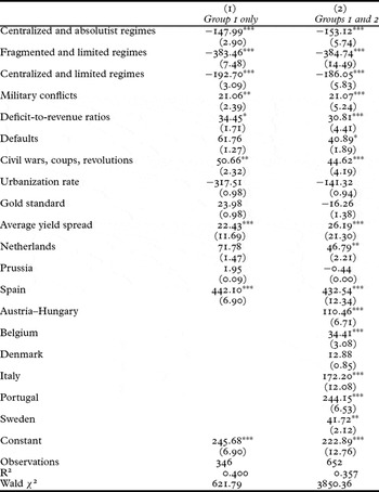
Table 6, which shows the results of the panel regressions, indicates that fragmented and absolutist regimes displayed significantly higher levels of sovereign credit risk than the other regime types. These findings held for group 1 countries only (column 1) and when group 2 countries were included (column 2). Ceteris paribus, the move to a centralized and absolutist regime decreased yield spreads by 148 to 153 basis points. This result suggests that the positive impact of new revenues outweighed the negative impact of executive consolidation of fiscal powers. The move to a centralized and limited regime decreased yield spreads by 186 to 193 basis points and the move to the fragmented and limited one by 383 to 385 basis points.Footnote 29 The findings were also robust to checks that used alternative regime classifications.Footnote 30
Regression results for political regimes and sovereign credit risk

Sources: See text.
*Significant at 10 percent level, **Significant at 5 percent level, ***Significant at 1 percent level.
Notes: The dependent variable is the annual yield spread with the British consol in basis points. The estimation technique is OLS with panel-corrected standard errors (PCSE). A common AR1 term was added to correct for serial correlation. Z-statistics in absolute values are in parentheses. Group 1: France, the Netherlands, Prussia and Spain. Group 2: Austria–Hungary, Belgium, Denmark, Italy, Portugal and Sweden. For details about the regression variables, see Appendix 2.
As expected, warfare had a significant negative impact on sovereign credit risk. Common shocks to European asset markets (e.g. large-scale military conflicts) were also associated with a significant increase in yield spreads. Domestic turmoil (civil wars, coups and revolutions) significantly worsened credit risk as well. Budget deficits and defaults also had negative effects, though to a lesser extent. Urbanization rates and gold standard adherence, meanwhile, had negligible impacts.Footnote 31 Finally, Spain, Austria–Hungary, Belgium, Italy, Portugal and Sweden all had notably larger spreads than did France.
Table 7, which displays the results of the structural break tests, reveals close relationships between major turning points in the yield spread series and political transformations that enhanced public finances. It also highlights the link between those innovations and military competition and conflicts. In the Netherlands, the best breaks came with the start of the Belgian War of Independence (1830), near limited government (1850), and with an unidentified event (1885). Limited government, which occurred during the Year of Revolutions in 1848, led to a significant decrease in spreads (29 percent).
Major breaks in yield spread series

Sources: See text.
*Significant at 10 percent level, **Significant at 5 percent level, ***Significant at 1 percent level.
Notes: The first column lists the relevant sample countries. The second column displays the years for the best three structural breaks over the years shown for each polity as determined by the algorithm described in the text. The third column reports the percentage change in yield spreads over the fifteen years following the break in question as compared to the fifteen years that preceded it. T-statistics in absolute values are in parentheses. The final column offers brief ‘explanations’ for the turning points, which are elaborated upon in the text. For England, yields on British consols rather than spreads were tested.
In France, the first turning point occurred with the July Revolution (1830) and the establishment of the short-lived constitutional regime (1830–47) that followed. Limited government led to a significant (73 percent) decrease in yield spreads. A second break coincided with the coup d'état and subsequent establishment of an authoritarian regime by Napoleon III at the start of the 1850s. As expected, it was associated with a significant (163 percent) increase in spreads. The final break (1871) came with the establishment of limited government (1870) and the Franco-Prussian War (1870–71). France's loss to Prussia appears to have offset the positive effects of limited government over the short term. Figure 1, however, indicates that French spreads fell steadily from 1872 onwards. By the 1880s, they resembled those under the constitutional ‘July’ regime from 50 years before.
In Portugal, the turning point that occurred in 1848 coincided with the establishment of limited government in 1851 as well as the 1840s colonial wars in Guinea. By the mid 1850s, Portuguese spreads had fallen by over 300 basis points. Other Portuguese breaks were associated with an unidentified event (1863) and the 1890s banking crisis. In Prussia, we observe turning points near the first Zollverein customs agreement in 1834, near the establishment of a centralized and limited regime in 1848 and the first Schleswig-Holstein War (1848–9), and with the Austro-Prussian War (1866). Section 4 examines why limited government in Prussia did not result in a spread reduction.
The best three turning points for Spain occurred at the end of the first Carlist Civil War (1833–9), near the start of the Naval War against Peru (1864), and near limited government (1879). Limited government, established at the end of the third Carlist Civil War (1872–6), was associated with a large decrease in yield spreads (52 percent). Curiously, fiscal centralization, which occurred in 1844 during a decade of reforms, was not included as one of the top Spanish breaks. Figure 4, however, shows that yield spreads fell by roughly 500 basis points in the decade or so that followed this political change.
Turning points in the English yield series, which began after the establishment of a centralized and limited regime, further highlight the role of military conflicts. The top three breaks came at the start of War of American Independence (1775) and near the start (1798) and finish (1815) of the Napoleonic Wars. In each case, we observe a significant increase in consol yields at the conflict's outbreak (1775, 1798) and a significant decrease at war's end (1815).
7. Conclusion
This article examines the relationship between political regimes and sovereign credit risk in Europe from 1750 to 1913. Panel regressions indicate that centralized and/or limited regimes were associated with significant creditworthiness improvements relative to fragmented and absolutist ones. Structural break tests that assume no a priori knowledge of possible turning points in the yield series support these conclusions.
Historical analysis reveals general patterns in the evolution of political regimes and public finances. Prior to the 1800s, the most urgent problem facing most polities was fiscal fragmentation. Since Old Regime monarchs were already ‘constrained’ by local tax authorities, it was not until after centralization that national parliaments became ‘the’ mechanism by which to hold crowns accountable.
We lose sight of this point when studying English financial history, which was exceptional. By managing to avoid the problems of severe fragmentation that hampered Continental countries for so long, England was in a better position for development. Our key lesson from history, then, is simple but powerful. Today's emerging economies must try to adopt fiscal structures that not only limit the power of executives to behave recklessly, but that also lend enough authority to central governments to collect sufficient tax funds.
Acknowledgements
This article is a revised version of the second chapter of my PhD dissertation (UCLA, 2006). I would like to offer my sincere gratitude to my graduate advisor, Jean-Laurent Rosenthal, as well as to Naomi Lamoreaux. I would also like to thank Kimberly Crawford, Giovanni Federico, Wantje Fritschy, Knick Harley, Philip Hoffman, Joost Jonker, Robert Margo, Marjolein t'Hart, Mark Weidenmier, Jaime Reis and Jan Luiten van Zanden for valuable suggestions and/or help with the construction of the data set. Albrecht Ritschl and two anonymous referees provided useful comments, as did seminar participants at the EHA Annual Meeting (2006), the Collegio Carlo Alberto, the Universidad Carlos III, IMT Lucca, UCLA, and the All-UC Group in Economic History Workshop (2005). Finally, I would like to thank IMT Lucca, the Institute for Humane Studies, and UCLA for financial support.
Appendix 1. Sources for the yield data
The abbreviation GFD denotes the Global Financial Database. For additional details, see the text.
Austria–Hungary. Austrian data on 10-year government bonds were drawn from the GFD. For 1874–9, the silver 5s bond was used; for 1880–1913, the gold 4s bond. For 1874–9, monthly data were used to compute yearly averages; for 1880–1913, weekly data. Yields were for bonds traded in London.
Belgium. Belgian data on 10-year government bonds were drawn from the GFD. For 1832–44, the 5 percent Belgian bond was used; for 1845–58, the 4.5 percent bond; for 1859 onwards, the 3 percent bond. For 1832–84, monthly data were used to compute yearly averages; for 1885–98, biweekly data; for 1889–1913, monthly data. Note that the resulting yield series matched up closely with annual observations (taken from the last day of trading each year) from Homer and Sylla (Reference Homer and Sylla1991). Yields were for bonds traded in Brussels.
Denmark. Danish data on 10-year government bonds were drawn from the GFD. For 1821–5 and 1852–8, the 5s bond was used; for 1825–52, the 3s bond; for 1864–94 the consolidated 4s bond. In 1895 the consolidated 4s bond was converted into 3.5 percent consols, which were used through 1913. Data were unavailable for 1859–63. Monthly data were used to compute yearly averages from 1821 to 1913. Yields were for bonds traded in London.
England. The British series on perpetual government bonds were drawn from the GFD. For 1750–3, the 3 percent yield on annuities was used. For 1754 onwards, the British consol was used, which paid 3 percent until 1888, 2.75 percent from 1889 to 1906, and 2.5 percent from 1907 to 1913. For 1750–1879, monthly data were used to compute yearly averages; for 1880–1913, weekly data. Note that the resulting yield series matched up closely with annual observations (taken from the last day of trading each year) from Homer and Sylla (Reference Homer and Sylla1991). Yields were for bonds traded in London.
France. No single debt instrument akin to the British consol existed in France prior to the nineteenth century, making it difficult to identify ‘the’ interest rate paid on government loans. Indeed, bonds could be perpetual or finite, redeemable or not, and repudiated when revenues ran thin. The eighteenth-century yield data that I used were collected by Velde and Weir (Reference Velde and Weir1992), who chose the October loan as the French asset that best captured yields on long-term government bonds from 1750 to 1793. Prior to 1770, the October loan was a private debt of the Compagnie des Indes. From 1770 onwards, it was a perpetual debt of the French government. From 1793 to 1796, the Paris Stock Exchange was closed off and on. Data for 1794–1800 were unvailable, though a perpetual 5 percent consolidated bond was issued in 1798. It continued to trade until 1825, when the French central government refunded it and issued a perpetual 3 percent bond, which became the primary government bond until 1949. Note that a new bond paying quarterly interest replaced the previous 3 percent one in 1862. French data for the nineteenth and twentieth centuries were supplied courtesy of Jean-Laurent Rosenthal for 1801–72 and drawn from the GFD for 1873–1913. For 1750–1879, monthly data were used to compute yearly averages; for 1880–1913, weekly data. Yields were for bonds traded on the Paris Stock Exchange.
Italy. Italian data on long-term government bonds were drawn from the GFD. The average maturity was six years. For 1862–99, the consolidated 5 percent bond was used; for 1900–13, the 3.5 percent consol bond. Monthly data were used to compute yearly averages from 1862 to 1913. Yields were for bonds traded in London.
The Netherlands. Public bonds in the Dutch Republic were issued by several authorities, including the Union itself, provinces, and cities. Joost Jonker, Oscar Gelderblom and Heleen Kole collected the Dutch data for 1780–1810. Prior to 1780, too little data existed to form a comprehensive series. For 1780–95, the source was the Dutch newspaper Maandelijksche Hollandsche, which reported yields on various government bonds from securities auctions in Amsterdam. The Holland and Westfriesland perpetual 2.5 percent bond was selected. Like the October loan in eighteenth-century France, this asset best captured long-term yield levels. For 1796–1813, the source was the Dutch newspaper Prijscourant der Effecten. In this case, perpetual 2.5 percent national bonds were used. Data were unavailable for 1812. In 1814, the entire national debt, with interest rates ranging from 1.25 to 7 percent, was converted into a single one at a rate of 2.5 percent. The data source for 1814–1913 was the GFD. For 1780–96, monthly data were used to compute yearly averages; for 1797–1812, biweekly data; for 1814–81, monthly data; for 1882, biweekly data; for 1883–1913, weekly data. Note that the resulting nineteenth-century yield series matched up closely with annual observations that came from the Dutch National Accounts. Nineteenth- and twentieth-century bonds were also traded in Amsterdam.
Portugal. Portuguese data on 10-year government bonds were drawn from the GFD. For 1823–95 and 1903–13, the 3 percent bond was used. Data were unavailable for 1903. Monthly data were used to compute yearly averages for 1823–1913. Note that the resulting yield series matched up closely with monthly observations gathered by hand from Le Moniteur Universel and The Economist for all available years from 1835 to 1870. Yields were for bonds traded in London.
Prussia. Prussian data on 10-year government bonds from 1815 to 1841 were drawn from the GFD. For 1842–69, however, this source used Bavarian bonds. Prussian data on 10-year government bonds were thus drawn from Homer and Sylla (Reference Homer and Sylla1991) during those years. 4s bonds were used, except for 1844–52, when 3.5s bonds were used due to a lack of data. The Prussian data on 10-year government bonds for 1870–1913 were also drawn from the GFD. Prussian 4 percent consols were used for 1870–97 and German 3 percent Imperial loans for 1898–1913. For 1815–41, monthly data were used to compute yearly averages; for 1842–69, annual data (taken from the last day of trading each year); for 1870–80, monthly data, for 1881–1913, weekly data. Note that the resulting yield series taken from the GFD matched up closely with annual observations (taken from the last day of trading each year) for 1815–41 and 1870–80 from Homer and Sylla (Reference Homer and Sylla1991). Yields were for bonds traded in Berlin.
Spain. As in Old Regime France, the Spanish crown issued a variety of disparate debt instruments prior to 1815 (see Tortella and Comìn Reference Tortella, Comín, Bordo and Cortés-Conde2001). However, the Spanish yields series did not begin until 1821. Data were for 10-year government bonds drawn from the GFD. For 1823–36, 5s bonds were used. For 1836–81, 3s bonds were used. In 1881, the 3s were converted into a 1 percent bond. In 1882, the 1 percent bond was converted into a 1.25 percent one, and later into a 4 percent one. The 4 percent bond was used from 1882 to 1913. Monthly data were used for 1821–1913 to compute yearly averages. Note that the resulting yield series matched up closely with monthly observations gathered by hand from Le Moniteur Universel and The Economist for 1823–70. London yields were used for the entire series except for 1913 when the Madrid yield was used.
Sweden. Swedish data on 10-year government bonds were drawn from the GFD. For 1868–78, the 5s bond was used; for 1878–94, the 4s bond; for 1894–1913, the 3s bond. Monthly data were used to compute yearly averages for 1868–1913. Note that the resulting yield series matched up closely with annual observations (taken from the last day of trading each year) from Homer and Sylla (Reference Homer and Sylla1991) for all available years from 1855 to 1913. Yields were for bonds traded in London.
Appendix 2. Regression variables
For additional details, see Sections 5 and 6 of the text.
The dependent variable is the spread between the average annual yield on long-term government bonds for each sample country and the average annual yield on the British consol as expressed in basis points.
The dummy variable for fragmented and absolutist political regimes takes a value of one for each year that a sample country possessed a fragmented and absolutist regime from 1750 to 1913. As the benchmark case, I omitted it from the regression specifications. The dummy variable for centralized and absolutist political regimes takes a value of one for each year that a sample country possessed a centralized and absolutist regime from 1750 to 1913. The dummy variable for fragmented and limited political regimes takes a value of one for each year that a sample country possessed a fragmented and limited regime from 1750 to 1913. There is only one such case among sample countries; for additional details, see Section 4. The dummy variable for centralized and limited political regimes takes a value of one for each year that a sample country possessed a centralized and limited regime from 1750 to 1913.
The country dummy variable takes a value of one to identify individual sample countries.
Wars and war years are from Clodfelter (Reference Clodfelter2002). All conflicts fought at least in part in Western Europe (as well as those fought at least in part in Eastern Europe so long as they involved at least one sample country) from 1750 to 1913 were included. Table A1 provides a complete list.
European military conflicts, 1750–1913

Source: Clodfelter (Reference Clodfelter2002).
Notes: Country abbreviations are Austria–Hungary (Ah), Belgium (Be), Bosnia (Bo), Corsica (Co), Denmark (Dk), England (En), France (Fr), Italy (It), the Netherlands (Nl), Poland (Pl), Portugal (Pt), Prussia (Pr), Russia (Ru), Sardinia (Sa), Spain (Sp), Sweden (Sw) and Turkey (Tr).
The default dummy variable takes a value of one for each year that a national government partially or fully defaulted on its publicly held debt from 1750 to 1913 according to Reinhart, Rogoff and Savastano (Reference Reinhart, Rogoff and Savastano2003) and Dincecco (Reference Dincecco2009b). Table A3 provides a complete list.
The deficit variable, taken from Dincecco (Reference Dincecco2009b), is the budget deficit-to-revenue ratio for each sample country for each available year from 1750 to 1913.
The dummy variable for civil wars, coups and revolutions takes a value of one for each year of civil war, coup or revolution within sample countries from 1750 to 1913 according to Dincecco (Reference Dincecco2009a). Table A2 provides a complete list. Insurrections, massacres, riots and uprisings were generally not included.
European civil wars, coups and revolutions, 1750–1913

Source: Dincecco (Reference Dincecco2009a).
Defaults in Europe, 1750–1913

Sources: Reinhart, Rogoff and Savastano (Reference Reinhart, Rogoff and Savastano2003) and Dincecco (Reference Dincecco2009b).
The urbanization variable calculates the urban population as a fraction of the total population for each sample country annually. All urban population figures are from De Vries (Reference De Vries1984). Figures for 1750 and 1800 are from appendix 3, pp. 305–37, and figures for 1850, 1890 and 1980 are from table 4.8, pp. 44–7, for cities with populations of at least 10,000 inhabitants through 1850, with at least 20,000 inhabitants in 1890, and with at least 100,000 inhabitants in 1980. All intermediate years were interpolated. De Vries provides urbanization figures for Germany rather than for Prussia and for Scandinavia rather than for Denmark or Sweden. Urbanization figures for Austria–Hungary include Bohemia. For country population sources, see Dincecco (Reference Dincecco2009a).
The per-capita GDP variable, which comes from Maddison (Reference Maddison2003), takes the natural logarithm of per-capita GDP in 1990 international Geary-Khamis dollars for sample countries from 1750 to 1913. Data were available for 1700 and 1820–1913. All intermediate years were interpolated. Maddison provides per-capita GDP figures for Germany rather than for Prussia.
The gold variable dummy variable takes a value of one for each year that a country was on gold according to Meissner (Reference Meissner2005), who employs a strict measure of gold adherence that chooses the year in which a currency became de facto and de jure convertible into gold. Adoption years were England, 1821; Portugal, 1854; Prussia, 1872; Denmark, 1873; Sweden, 1873; the Netherlands, 1875; Belgium, 1878; France, 1878; and Italy, 1884. Neither Austria–Hungary nor Spain formally adopted the gold standard prior to 1913.
The average spread variable is the average yield spread in basis points for all available sample countries over the ‘safe’ British consol for each year from 1750 to 1913.