1 Introduction
Many different concepts for wave energy conversion have been proposed (Clément et al. Reference Clément, McCullen, Falcão, de, Fiorentino, Gardner, Hammarlund, Lemonis, Lewis and Nielsen2002; Drew, Plummer & Sahinkaya Reference Drew, Plummer and Sahinkaya2009; Rusu & Onea Reference Rusu and Onea2018). However, compared with other renewable energy technologies, such as solar, wind or tidal, wave power is rather immature, and relatively few wave energy converters (WECs) have achieved fully commercial operation (Drew et al. Reference Drew, Plummer and Sahinkaya2009; Astariz & Iglesias Reference Astariz and Iglesias2015; Mustapa et al. Reference Mustapa, Yaakob, Ahmed, Rheem, Koh and Adnan2017).
Among the various wave energy conversion concepts, the oscillating water column (OWC) is probably the most extensively investigated and best developed (Heath Reference Heath2012; Falcão & Henriques Reference Falcão and Henriques2016). An OWC is generally composed of a hollow chamber with its bottom open to the sea below the waterline. Subjected to ocean waves, the water column enclosed by the chamber moves up and down, applying pressure on the air within the chamber. The air is forced in and out of the chamber through a turbine installed at the top of the OWC, allowing for power extraction.
The cost of power is the major limitation to the uptake of WECs in commercial operation (Heath Reference Heath2012; Di Lauro et al. Reference Di Lauro, Lara, Maza, Losada, Contestabile and Vicinanza2019). This is a general issue with wave energy, not specific to OWC technology. A number of efforts have been made to achieve commercialization of OWCs (Viviano et al. Reference Viviano, Naty, Foti, Bruce, Allsop and Vicinanza2016; Pawitan et al. Reference Pawitan, Dimakopoulos, Vicinanza, Allsop and Bruce2019). The integration of OWCs into coastal structures, such as breakwaters, jetties and piers, or along sections of the coast, presents an effective way to increase significantly the attractiveness of wave power exploitation. The fact that the capture factor of WECs may be enhanced by their deployment along the coast (which may be referred to, for simplicity, as the coast effect) was reported for flap-type WECs by Sarkar, Renzi & Dias (Reference Sarkar, Renzi and Dias2015) and Michele, Sammarco & d’Errico (Reference Michele, Sammarco and d’Errico2016), and also for oscillating buoys by Evans (Reference Evans1988), Zhao et al. (Reference Zhao, Ning, Johanning and Teng2018) and Zhang & Ning (Reference Zhang and Ning2019). In this way, the economics of the OWC can be enhanced thanks to cost-sharing benefits, including construction, installation and maintenance (Boccotti Reference Boccotti2007; Heras-Saizarbitoria, Zamanillo & Laskurain Reference Heras-Saizarbitoria, Zamanillo and Laskurain2013; Arena et al. Reference Arena, Romolo, Malara, Fiamma and Laface2017; Mustapa et al. Reference Mustapa, Yaakob, Ahmed, Rheem, Koh and Adnan2017). Reliability and survivability of the OWC can be improved as well, allowing power extraction during large wave conditions.
Many theoretical investigations have been devoted to wave power extraction by coast/breakwater-integrated OWCs. Evans & Porter (Reference Evans and Porter1995) proposed a two-dimensional (2-D) theoretical model to study the performance of an onshore OWC device that consists of a thin vertical surface-piercing lip in front of a vertical wall. It was illustrated that, by choosing proper submergence of the lip and the spacing distance between the lip and the wall, the incident wave power can be captured efficiently. The performance of a thin-walled OWC installed either at the tip of a thin fixed breakwater or along a straight coast was considered by Martins-Rivas & Mei (Reference Martins-Rivas and Mei2009a ,Reference Martins-Rivas and Mei b ), who developed theoretical models based on the linear potential flow theory to solve the three-dimensional (3-D) wave radiation/diffraction problems. To deal with the singular behaviours in the velocity field across the gap under the thin wall of OWC chamber, an integral equation for the horizontal velocity under the wall was employed in their models. The extracted power of the OWC at the tip of a thin breakwater was found to be reasonably insensitive to the incident wave direction, whereas the response of the OWC installed on a straight coast was strongly dependent on wave direction. The best performance occurred under normal incidence for most frequencies. Wave reflection at the coast means that the power captured by the OWC can be doubled. Lovas, Mei & Liu (Reference Lovas, Mei and Liu2010) extended the theoretical model by Martins-Rivas & Mei (Reference Martins-Rivas and Mei2009a ,Reference Martins-Rivas and Mei b ) into a more general model that can be applied to more complex situations, i.e. a thin-walled OWC installed at a coastal corner. The captured power by the OWC at a concave corner was found to be significantly greater than that when the OWC was installed at the tip of a convex corner of right angle.
More recently, Zheng, Zhang & Iglesias (Reference Zheng, Zhang and Iglesias2019) developed a theoretical model of a coast/breakwater-integrated OWC, in which the effect of the thickness of the OWC chamber wall was considered. Subjected to a fixed outer radius, the thinner the chamber wall, the larger and broader the main peaks of the frequency response of wave power capture width. Numerical and physical studies on a coast/breakwater-integrated OWC can be found in Morris-Thomas, Irvin & Thiagarajan (Reference Morris-Thomas, Irvin and Thiagarajan2007), He, Huang & Law (Reference He, Huang and Law2012), Zhang, Zou & Greaves (Reference Zhang, Zou and Greaves2012), López & Iglesias (Reference López and Iglesias2014), Elhanafi et al. (Reference Elhanafi, Fleming, Macfarlane and Leong2016), Falcão, Henriques & Gato (Reference Falcão, Henriques and Gato2016), López et al. (Reference López, Pereiras, Castro and Iglesias2016), He, Leng & Zhao (Reference He, Leng and Zhao2017) and Howe & Nader (Reference Howe and Nader2017). However, most of these studies are focused on 2-D problems, and therefore miss fundamental dynamics related to direction changes in wave diffraction and radiation from complex-shaped structures.
In order to fully harness the available wave power in a region and to produce large quantities of energy for electrical grids, wave farms, i.e. arrays of OWCs, are likely to be deployed. For these OWCs deployed not far away from each other, cost-sharing benefits of installation and electrical power transmission can be made as well. On the basis of an analytical solution of hydrodynamic problems from an oscillating circular patch on the water surface, Nihous (Reference Nihous2012) presented a model to predict wave power absorption from an array of OWCs. The OWC chamber was assumed to have a sufficiently shallow draught; thus diffraction effects were neglected in the model. A finite array of fixed OWCs without the restriction of shallow draught was considered by Nader et al. (Reference Nader, Zhu, Cooper and Stappenbelt2012) by applying a 3-D finite element method model. The complexity of hydrodynamic interactions between the OWCs within the array was highlighted. Later, a more realistic model with the air compressibility inside the OWC chamber taken into account was proposed (Sarmento & Falcão Reference Sarmento and Falcão1985; Nader, Zhu & Cooper Reference Nader, Zhu and Cooper2014; López et al. Reference López, Carballo, Taveira-Pinto and Iglesias2020). The results showed that, for some certain wave frequencies, more power can be harnessed by the array of fixed OWCs compared with the total power that the same number of OWCs working in isolation could extract. Recently, Konispoliatis & Mavrakos (Reference Konispoliatis and Mavrakos2016) developed an efficient theoretical model to investigate the performance of an array of free-floating OWCs. Major improvements in terms of extracted power were demonstrated for arrays with certain spacings between the OWCs. More recently, the hydrodynamic characteristics of a hybrid wave farm consisting of both OWCs and point-absorber WECs were investigated by Zheng, Zhang & Iglesias (Reference Zheng, Zhang and Iglesias2018).
Apart from the integration of OWCs into coastal structures and the deployment of OWCs in an array, various studies have also been carried out on the development of individual OWCs (López et al. Reference López, Pereiras, Castro and Iglesias2014; Pereiras et al. Reference Pereiras, López, Castro and Iglesias2015; Henriques et al. Reference Henriques, Gato, Falcão, de, Robles and Faÿ2016; Elhanafi et al. Reference Elhanafi, Fleming, Macfarlane and Leong2017; Kurniawan et al. Reference Kurniawan, Chaplin, Greaves and Hann2017; Ning, Zhou & Zhang Reference Ning, Zhou and Zhang2018; Sheng & Lewis Reference Sheng and Lewis2018; He et al. Reference He, Zhang, Zhao, Zheng and Iglesias2019).
To the authors’ knowledge, most of the previous research work on OWCs has been focused on the investigation of either a single coast-integrated/offshore OWC or an array of offshore OWCs. In this article, the concept of integrating multiple OWCs into a straight coast is proposed. The chamber of each OWC mainly consists of a hollow vertical circular cylinder, which is cut away such that it is half open to the sea from a finite submergence to the seabed. To evaluate the hydrodynamic performance of these coast-integrated OWCs, a 3-D theoretical model is developed based on the linear potential flow theory and eigenfunction matching method. The water depth is assumed to be constant, in order to simplify the wave conditions. The effect of a Wells turbine installed at the top of each OWC together with the air compressibility are taken into account by means of a linear power take-off (PTO) system. Different from most of the previous reviewed 3-D theoretical models for a single coast-integrated thin-walled OWC, the present model can be used to study wave power extraction from multiple coast-integrated OWCs without the thin-wall restriction, i.e. the effect of the wall thickness of the OWC chamber is taken into consideration. The performance of the multiple coast-integrated OWC system is compared with that of a single individual coast-integrated OWC, and also with that of single and multiple offshore OWCs, which consists of a stationary hollow vertical cylinder located in the open sea with the whole cylinder cut off at a finite distance from the seabed. The theoretical model is applied to explore the influences of incident wave direction, chamber size (i.e. radius, wall thickness and submergence), spacing distance between the OWCs and the number of OWCs on power extraction systematically.
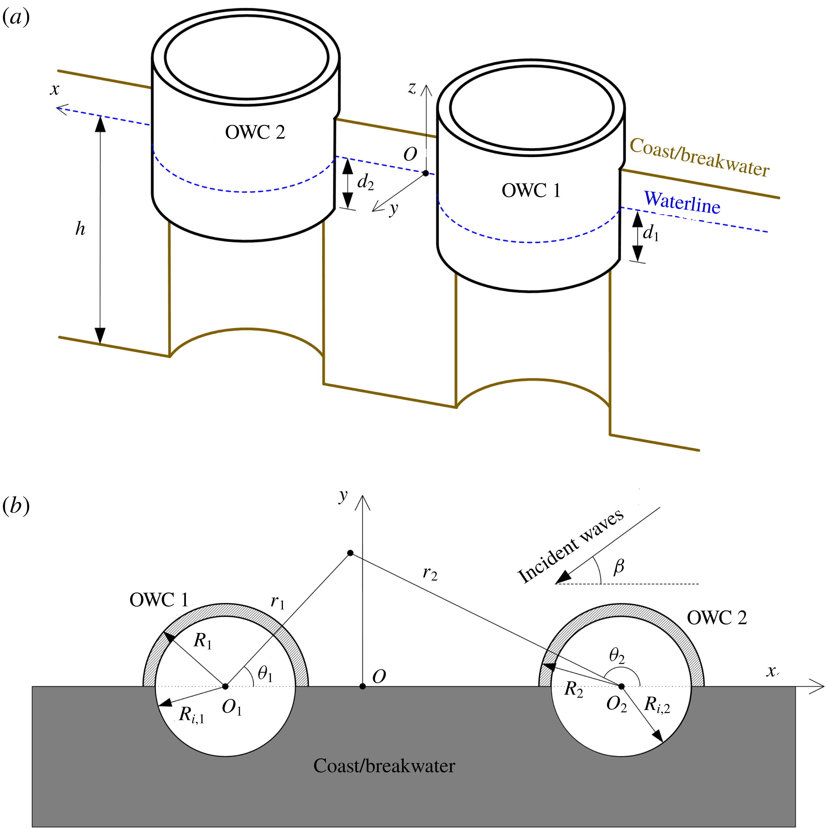
Definition sketch: (a) general layout of a pair of OWCs; (b) plan section with key dimensions.

2 Mathematical model
In the model, a number (
 $N$
) of OWCs are conceptually installed along a straight coast in water of finite depth
 $h$
(see figure 1, where
 $N=2$
is taken as an example). A global Cartesian coordinate system
 $Oxyz$
is adopted with the
 $Oxy$
plane at the mean water level and the
 $Oxz$
plane at the sidewall of the coast. For the
 $N$
vertical circular OWC chambers, the OWCs are numbered along the
 $Ox$
axis in ascending order, and
 $N$
local cylindrical coordinate systems,
 $O_{n}r_{n}\unicode[STIX]{x1D703}_{n}z_{n}$
, are defined with their origins
 $O_{n}$
at the central vertical axis of the
 $n$
th OWC
 $(n=1,2,\ldots ,N)$
. The
 $O_{n}$
can be defined in Cartesian coordinate system
 $Oxyz$
as (
 $x_{n},0,0$
). In addition,
 $R_{n}$
,
 $R_{i,n}$
and
 $d_{n}$
denote the outer radius, inner radius and submergence of the
 $n$
th OWC chamber, respectively; and
 $D_{n}$
represents the distance between
 $O_{n}$
and
 $O_{n+1}$
.
For the coast-integrated OWCs subjected to regular incident waves with small wave steepness propagating in the direction of
 $\unicode[STIX]{x1D6FD}$
relative to the coast (see figure 1), in the framework of linear potential flow theory, the fluid flow in the water domain is described by the velocity potential
 $$\begin{eqnarray}\unicode[STIX]{x1D719}(x,y,z,t)=\text{Re}[\unicode[STIX]{x1D6F7}(x,y,z)\text{e}^{-\text{i}\unicode[STIX]{x1D714}t}].\end{eqnarray}$$
Here
 $\unicode[STIX]{x1D6F7}$
is a complex spatial velocity potential independent of time, which needs to satisfy Laplace’s equation in the fluid, in addition to certain linear boundary conditions, which will be given shortly; i is the imaginary unit;
 $\unicode[STIX]{x1D714}$
denotes the circular frequency of incident waves; and
 $t$
is the time. The linear potential flow theory is not suitable for extreme waves, given that it does not account for either the viscous effect or the nonlinear wave dynamics.
Under linear theory, the spatial velocity potential
 $\unicode[STIX]{x1D6F7}$
may be decomposed as the sum of scattering and radiation potentials, i.e.
 $$\begin{eqnarray}\unicode[STIX]{x1D6F7}=\unicode[STIX]{x1D6F7}_{0}+\mathop{\sum }_{n=1}^{N}p_{n}\unicode[STIX]{x1D6F7}_{n},\end{eqnarray}$$
where
 $\unicode[STIX]{x1D6F7}_{0}$
is the scattering spatial velocity potential representing the wave field when the coast-integrated OWCs with the top of each chamber entirely open to the air (i.e. no dynamic air pressure) are subjected to the incident waves;
 $p_{n}$
is the complex air pressure amplitude inside the
 $n$
th OWC chamber; and
 $\unicode[STIX]{x1D6F7}_{n}$
represents the spatial velocity potential due to a unit air pressure oscillation inside the
 $n$
th OWC chamber while all the others are at rest.
Outside the OWCs,
 $\unicode[STIX]{x1D6F7}_{0}$
can be taken as the sum of two parts,
 $\unicode[STIX]{x1D6F7}_{0}=\unicode[STIX]{x1D6F7}_{I}+\unicode[STIX]{x1D6F7}_{D}$
, where
 $\unicode[STIX]{x1D6F7}_{I}$
is the spatial velocity potential representing the wave field due to the incident waves in the absence of OWCs, which includes both the incident plane wave and a plane wave reflected by the wall, and
 $\unicode[STIX]{x1D6F7}_{D}$
is the diffracted spatial velocity potential due to the presence of the OWCs. In the
 $n$
th local cylindrical coordinate system
 $O_{n}r_{n}\unicode[STIX]{x1D703}_{n}z$
,
 $\unicode[STIX]{x1D6F7}_{I}$
can be written as (Zheng & Zhang Reference Zheng and Zhang2015)
 $$\begin{eqnarray}\unicode[STIX]{x1D6F7}_{I}(r_{n},\unicode[STIX]{x1D703}_{n},z)=-\frac{2\text{i}gA}{\unicode[STIX]{x1D714}}\frac{Z_{0}(z)}{Z_{0}(0)}\text{e}^{-\text{i}k_{0}x_{n}\cos \unicode[STIX]{x1D6FD}}\mathop{\sum }_{m=0}^{\infty }\unicode[STIX]{x1D700}_{m}(-\text{i})^{m}\text{J}_{m}(k_{0}r_{n})\cos (m\unicode[STIX]{x1D6FD})\cos (m\unicode[STIX]{x1D703}_{n}).\end{eqnarray}$$
Here
 $A$
is the amplitude of incident waves;
 $g$
denotes the gravitational acceleration;
 $\unicode[STIX]{x1D700}_{m}=1$
for
 $m=0$
, whereas
 $\unicode[STIX]{x1D700}_{m}=2$
for
 $m>0$
;
 $k_{0}$
is the wavenumber, which satisfies the dispersion relation
 $\unicode[STIX]{x1D714}^{2}=gk_{0}\tanh (k_{0}h)$
;
 $\text{J}_{m}$
denotes the Bessel function of order
 $m$
; and
 $Z_{0}(z)$
is an eigenfunction given by
 $$\begin{eqnarray}Z_{0}(z)=N_{0}^{-1/2}\cosh [k_{0}(z+h)],\quad N_{0}=\frac{1}{2}\left[1+\frac{\sinh (2k_{0}h)}{2k_{0}h}\right].\end{eqnarray}$$
The governing equation in the water domain, the free-surface boundary conditions, and the body boundary conditions that
 $\unicode[STIX]{x1D6F7}_{\unicode[STIX]{x1D712}}~(\unicode[STIX]{x1D712}=0,1,2,\ldots ,N)$
should satisfy are given as follows:
 $$\begin{eqnarray}\displaystyle & \displaystyle \unicode[STIX]{x1D6FB}^{2}\unicode[STIX]{x1D6F7}_{\unicode[STIX]{x1D712}}=0,\quad \text{in water}, & \displaystyle\end{eqnarray}$$
 $$\begin{eqnarray}\displaystyle & \displaystyle \frac{\unicode[STIX]{x2202}\unicode[STIX]{x1D6F7}_{\unicode[STIX]{x1D712}}}{\unicode[STIX]{x2202}n}=0,\quad \text{on all solid boundaries}, & \displaystyle\end{eqnarray}$$
 $$\begin{eqnarray}\displaystyle & & \displaystyle \left(\frac{\unicode[STIX]{x2202}\unicode[STIX]{x1D6F7}_{\unicode[STIX]{x1D712}}}{\unicode[STIX]{x2202}z}-\frac{\unicode[STIX]{x1D714}^{2}}{g}\unicode[STIX]{x1D6F7}_{\unicode[STIX]{x1D712}}\right)\biggm\vert_{z=0}=\unicode[STIX]{x1D6FF}_{\unicode[STIX]{x1D712},n}\frac{\text{i}\unicode[STIX]{x1D714}}{\unicode[STIX]{x1D70C}g},\nonumber\\ \displaystyle & & \displaystyle \qquad \text{on the water surface inside the }n\text{th OWC chamber},\end{eqnarray}$$
 $$\begin{eqnarray}\displaystyle & & \displaystyle \left(\frac{\unicode[STIX]{x2202}\unicode[STIX]{x1D6F7}_{\unicode[STIX]{x1D712}}}{\unicode[STIX]{x2202}z}-\frac{\unicode[STIX]{x1D714}^{2}}{g}\unicode[STIX]{x1D6F7}_{\unicode[STIX]{x1D712}}\right)\biggm\vert_{z=0}=0,\nonumber\\ \displaystyle & & \displaystyle \qquad \text{on the water surface outside the }n\text{th OWC chamber},\end{eqnarray}$$
in which
 $\unicode[STIX]{x1D6FF}_{\unicode[STIX]{x1D712},n}$
is the Kronecker delta function, which is equal to 1 when
 $\unicode[STIX]{x1D712}=n$
, and is equal to 0 otherwise; and
 $\unicode[STIX]{x1D70C}$
represents the water density.
Additionally, it is required that
 $\unicode[STIX]{x1D6F7}_{D}$
and
 $\unicode[STIX]{x1D6F7}_{\unicode[STIX]{x1D712}}$
(
 $\unicode[STIX]{x1D712}=1,2,\ldots ,N$
) are outgoing for
 $r_{n}\rightarrow \infty$
.
3 Solution of scattering and radiated potentials
3.1 Scattering and radiated spatial potentials in different regions
The general solution of the potential
 $\unicode[STIX]{x1D6F7}_{\unicode[STIX]{x1D712}}$
in the region enclosed by the
 $n$
th OWC, i.e.
 $r_{n}\in [0,R_{i,n}]$
,
 $\unicode[STIX]{x1D703}_{n}\in [0,2\unicode[STIX]{x03C0}]$
,
 $z\in [-h,0]$
, is formally expressed as
 $$\begin{eqnarray}\unicode[STIX]{x1D6F7}_{\unicode[STIX]{x1D712},n}^{in}(r_{n},\unicode[STIX]{x1D703}_{n},z)=\mathop{\sum }_{m=-\infty }^{\infty }\mathop{\sum }_{l=0}^{\infty }\frac{\tilde{\text{I}}_{m}(k_{l}r_{n})}{k_{l}\tilde{\text{I}^{\prime }}_{m}(k_{l}R_{i,n})}A_{m,l}^{\unicode[STIX]{x1D712},n}Z_{l}(z)\text{e}^{\text{i}m\unicode[STIX]{x1D703}_{n}}-\text{i}\frac{\unicode[STIX]{x1D6FF}_{\unicode[STIX]{x1D712},n}}{\unicode[STIX]{x1D70C}\unicode[STIX]{x1D714}}.\end{eqnarray}$$
Here
 $A_{m,l}^{\unicode[STIX]{x1D712},n}$
are the unknown coefficients to be solved;
 $$\begin{eqnarray}\tilde{\text{I}}_{m}(k_{l}r_{n})=\left\{\begin{array}{@{}ll@{}}\text{J}_{m}(k_{l}r_{n}),\quad & l=0,\\ \text{I}_{m}(k_{l}r_{n}),\quad & l=1,2,3,\ldots ,\end{array}\right.\end{eqnarray}$$
in which
 $\text{I}_{m}$
denotes the modified Bessel function of the first kind of order
 $m$
;
 $k_{l}$
is the eigenvalue, which is given by (e.g. Falnes Reference Falnes2002)
 $$\begin{eqnarray}\unicode[STIX]{x1D714}^{2}=-gk_{l}\tan (k_{l}h),\quad l=1,2,3,\ldots ;\end{eqnarray}$$
and the corresponding eigenfunction
 $Z_{l}(z)$
is defined by
 $$\begin{eqnarray}Z_{l}(z)=N_{l}^{-1/2}\cos [k_{l}(z+h)],\quad N_{l}=\frac{1}{2}\left[1+\frac{\sin (2k_{l}h)}{2k_{l}h}\right],\quad l=1,2,3,\ldots .\end{eqnarray}$$
The eigenfunctions
 $Z_{0}(z)$
and
 $Z_{l}(z)$
, as given in (2.4) and (3.4), form a complete orthogonal set in
 $z\in [-h,0]$
:
 $$\begin{eqnarray}\int _{-h}^{0}Z_{m}(z)Z_{l}(z)\,\text{d}z=h\unicode[STIX]{x1D6FF}_{m,l},\quad m,l=0,1,2,3,\ldots .\end{eqnarray}$$
In the region beneath the
 $n$
th OWC chamber wall, i.e.
 $r_{n}\in [R_{i,n},R_{n}]$
,
 $\unicode[STIX]{x1D703}_{n}\in [0,\unicode[STIX]{x03C0}]$
,
 $z\in [-h,-d_{n}],$
the potential
 $\unicode[STIX]{x1D6F7}_{\unicode[STIX]{x1D712}}$
can be expressed as
 $$\begin{eqnarray}\displaystyle \unicode[STIX]{x1D6F7}_{\unicode[STIX]{x1D712},n}^{ring}(r_{n},\unicode[STIX]{x1D703}_{n},z) & = & \displaystyle \mathop{\sum }_{m=0}^{\infty }\left[F_{m,0}^{\unicode[STIX]{x1D712},n}(r_{n})+\mathop{\sum }_{l=1}^{\infty }\left(C_{m,l}^{\unicode[STIX]{x1D712},n}\frac{\text{I}_{m}(\unicode[STIX]{x1D6FD}_{n,l}r_{n})}{\text{I}_{m}(\unicode[STIX]{x1D6FD}_{n,l}R_{n})}\right.\right.\nonumber\\ \displaystyle & & \displaystyle +\left.\left.D_{m,l}^{\unicode[STIX]{x1D712},n}\frac{\text{K}_{m}(\unicode[STIX]{x1D6FD}_{n,l}r_{n})}{\text{K}_{m}(\unicode[STIX]{x1D6FD}_{n,l}R_{n})}\right)\cos [\unicode[STIX]{x1D6FD}_{n,l}(z+h)]\right]\cos (m\unicode[STIX]{x1D703}_{n}),\end{eqnarray}$$
which satisfies the no-flux boundary condition on the coast (
 $\unicode[STIX]{x1D703}_{n}=0$
and
 $\unicode[STIX]{x03C0}$
). Therein,
 $$\begin{eqnarray}F_{m,0}^{\unicode[STIX]{x1D712},n}(r_{n})=\left\{\begin{array}{@{}ll@{}}\displaystyle C_{m,0}^{\unicode[STIX]{x1D712},n}+D_{m,0}^{\unicode[STIX]{x1D712},n}\left[1+\ln \left(\frac{r_{n}}{R_{n}}\right)\right],\quad & m=0,\\ \displaystyle C_{m,0}^{\unicode[STIX]{x1D712},n}\left(\frac{r_{n}}{R_{n}}\right)^{|m|}+D_{m,0}^{\unicode[STIX]{x1D712},n}\left(\frac{r_{n}}{R_{n}}\right)^{-|m|},\quad & m\neq 0,\end{array}\right.\end{eqnarray}$$
in which
 $C_{m,l}^{\unicode[STIX]{x1D712},n}$
and
 $D_{m,l}^{\unicode[STIX]{x1D712},n}$
are the unknown coefficients to be determined;
 $\text{K}_{m}$
is the modified Bessel function of the second kind of order
 $m$
; and
 $\unicode[STIX]{x1D6FD}_{n,l}$
is the
 $l$
th eigenvalue given by
 $$\begin{eqnarray}\unicode[STIX]{x1D6FD}_{n,l}=\frac{l\unicode[STIX]{x03C0}}{h-d_{n}},\quad l=0,1,2,3,\ldots .\end{eqnarray}$$
In the region outside the OWC chambers and in front of the coast extending towards infinite distance horizontally, i.e.
 $r_{n}\in [R_{n},\infty ]$
,
 $\unicode[STIX]{x1D703}_{n}\in [0,\unicode[STIX]{x03C0}]$
,
 $z\in [-h,0]$
, the potential
 $\unicode[STIX]{x1D6F7}_{\unicode[STIX]{x1D712}}$
can be expressed as
 $$\begin{eqnarray}\unicode[STIX]{x1D6F7}_{\unicode[STIX]{x1D712}}^{out}(r_{n},\unicode[STIX]{x1D703}_{n},z)=\unicode[STIX]{x1D6FF}_{\unicode[STIX]{x1D712},0}\unicode[STIX]{x1D6F7}_{I}+\mathop{\sum }_{j=1}^{N}\unicode[STIX]{x1D6F7}_{\unicode[STIX]{x1D712},j}^{out},\end{eqnarray}$$
where
 $\unicode[STIX]{x1D6F7}_{\unicode[STIX]{x1D712},j}^{out}$
represents the velocity potential component diffracted/radiated from the
 $j$
th OWC, and it can be written in the
 $j$
th local cylindrical coordinate
 $O_{j}r_{j}\unicode[STIX]{x1D703}_{j}z$
as
 $$\begin{eqnarray}\unicode[STIX]{x1D6F7}_{\unicode[STIX]{x1D712},j}^{out}(r_{j},\unicode[STIX]{x1D703}_{j},z)=\mathop{\sum }_{m=0}^{\infty }\mathop{\sum }_{l=0}^{\infty }E_{m,l}^{\unicode[STIX]{x1D712},j}\frac{\tilde{\text{K}}_{m}(k_{l}r_{j})}{\tilde{\text{K}}_{m}(k_{l}R_{j})}\cos (m\unicode[STIX]{x1D703}_{j})Z_{l}(z),\end{eqnarray}$$
which satisfies the no-flux boundary condition on the coast (
 $\unicode[STIX]{x1D703}_{j}=0$
and
 $\unicode[STIX]{x03C0}$
). Here
 $E_{m,l}^{\unicode[STIX]{x1D712},j}$
are the unknown coefficients to be determined; and
 $$\begin{eqnarray}\tilde{\text{K}}_{m}(k_{l}r_{j})=\left\{\begin{array}{@{}ll@{}}\text{H}_{m}(k_{l}r_{j}),\quad & l=0,\\ \text{K}_{m}(k_{l}r_{j}),\quad & l=1,2,3,\ldots ,\end{array}\right.\end{eqnarray}$$
where
 $\text{H}_{m}$
denotes the Hankel function of the first kind of order
 $m$
.
Following Graf’s addition theorem for Bessel functions (Abramowitz & Stegun Reference Abramowitz and Stegun1964),
 $$\begin{eqnarray}\displaystyle & & \displaystyle \tilde{\text{K}}_{m}(k_{l}r_{j})\cos (m\unicode[STIX]{x1D703}_{j})\nonumber\\ \displaystyle & & \displaystyle \quad =\mathop{\sum }_{m^{\prime }=-\infty }^{\infty }\tilde{\text{K}}_{m+m^{\prime }}(k_{l}R_{jn})\tilde{\text{I}}_{m^{\prime }}(k_{l}r_{n})\text{e}^{\text{i}(m\unicode[STIX]{x1D6FC}_{jn}+m^{\prime }\unicode[STIX]{x1D6FC}_{nj})}\cos (m^{\prime }\unicode[STIX]{x1D703}_{n}),\quad r_{n}\leqslant R_{jn},\end{eqnarray}$$
where
 $R_{jn}$
and
 $\unicode[STIX]{x1D6FC}_{jn}$
denote the norm and the angle of vector
 $\overrightarrow{O_{j}O_{n}}$
, respectively. Therefore, the expression of
 $\unicode[STIX]{x1D6F7}_{\unicode[STIX]{x1D712},j}^{out}$
can be transformed from the
 $j$
th local cylindrical coordinate into the
 $n$
th one, and (3.9) is ultimately expressed in the local cylindrical coordinate
 $O_{n}r_{n}\unicode[STIX]{x1D703}_{n}z$
by
 $$\begin{eqnarray}\displaystyle & & \displaystyle \unicode[STIX]{x1D6F7}_{\unicode[STIX]{x1D712}}^{out}(r_{n},\unicode[STIX]{x1D703}_{n},z)=\unicode[STIX]{x1D6FF}_{\unicode[STIX]{x1D712},0}\unicode[STIX]{x1D6F7}_{I}+\mathop{\sum }_{m=0}^{\infty }\mathop{\sum }_{l=0}^{\infty }E_{m,l}^{\unicode[STIX]{x1D712},n}\frac{\tilde{\text{K}}_{m}(k_{l}r_{n})}{\tilde{\text{K}}_{m}(k_{l}R_{n})}\cos (m\unicode[STIX]{x1D703}_{n})Z_{l}(z)\nonumber\\ \displaystyle & & \displaystyle \quad +\,\mathop{\sum }_{\substack{ j=1, \\ j\neq n}}^{N}\mathop{\sum }_{m=0}^{\infty }\mathop{\sum }_{l=0}^{\infty }\frac{E_{m,l}^{\unicode[STIX]{x1D712},j}Z_{l}(z)}{\tilde{\text{K}}_{m}(k_{l}R_{j})}\mathop{\sum }_{m^{\prime }=-\infty }^{\infty }\tilde{\text{K}}_{m+m^{\prime }}(k_{l}R_{jn})\tilde{\text{I}}_{m^{\prime }}(k_{l}r_{n})\text{e}^{\text{i}(m\unicode[STIX]{x1D6FC}_{jn}+m^{\prime }\unicode[STIX]{x1D6FC}_{nj})}\cos (m^{\prime }\unicode[STIX]{x1D703}_{n}),\nonumber\\ \displaystyle & & \displaystyle \qquad \text{for }r_{n}\leqslant R_{jn}.\end{eqnarray}$$
3.2 Method of computation for unknown coefficients
It is easy to check that the governing equation and all the boundary conditions given in (2.5)–(2.8), except the no-flux condition on the inner and outer cylindrical surfaces of each OWC chamber
 $r_{n}=R_{n}$
and
 $r_{n}=R_{i,n}$
, have been satisfied by the scattering and radiated spatial potentials in different regions, as expressed in § 3.1, regardless of the values of the unknown coefficients. Note that the no-flux condition at
 $r_{n}=R_{n}$
and
 $r_{n}=R_{i,n}$
, together with the pressure and velocity continuity conditions on the interfaces of each two adjacent regions, should be satisfied as well, which can be applied to solve the unknown coefficients.
The continuity conditions for the scattering and radiated spatial potentials are given as follows:
(1) Continuity of normal velocity at the boundary
 $r_{n}=R_{i,n}$
:
 $$\begin{eqnarray}\frac{\unicode[STIX]{x2202}\unicode[STIX]{x1D6F7}_{\unicode[STIX]{x1D712},n}^{in}}{\unicode[STIX]{x2202}r_{n}}\biggm\vert_{r_{n}=R_{i,n}}=\left\{\begin{array}{@{}ll@{}}0,\quad & z\in [-d_{n},0],\unicode[STIX]{x1D703}_{n}\in [0,\unicode[STIX]{x03C0}],\\ \quad & \text{and }z\in [-h,0],\unicode[STIX]{x1D703}_{n}\in [\unicode[STIX]{x03C0},2\unicode[STIX]{x03C0}],\\ \displaystyle \frac{\unicode[STIX]{x2202}\unicode[STIX]{x1D6F7}_{\unicode[STIX]{x1D712},n}^{ring}}{\unicode[STIX]{x2202}r_{n}}\biggm\vert_{r_{n}=R_{i,n}},\quad & z\in [-h,-d_{n}],\unicode[STIX]{x1D703}_{n}\in [0,\unicode[STIX]{x03C0}].\end{array}\right.\end{eqnarray}$$
(2) Continuity of normal velocity at the boundary
 $r_{n}=R_{n}$
:
 $$\begin{eqnarray}\frac{\unicode[STIX]{x2202}\unicode[STIX]{x1D6F7}_{\unicode[STIX]{x1D712},n}^{out}}{\unicode[STIX]{x2202}r_{n}}\biggm\vert_{r_{n}=R_{n}}=\left\{\begin{array}{@{}ll@{}}0,\quad & z\in [-d_{n},0],\unicode[STIX]{x1D703}_{n}\in [0,\unicode[STIX]{x03C0}],\\ \displaystyle \frac{\unicode[STIX]{x2202}\unicode[STIX]{x1D6F7}_{\unicode[STIX]{x1D712},n}^{ring}}{\unicode[STIX]{x2202}r_{n}}\biggm\vert_{r_{n}=R_{n}},\quad & z\in [-h,-d_{n}],\unicode[STIX]{x1D703}_{n}\in [0,\unicode[STIX]{x03C0}].\end{array}\right.\end{eqnarray}$$
(3) Continuity of pressure at the boundary
 $r_{n}=R_{i,n}$
:
 $$\begin{eqnarray}\unicode[STIX]{x1D6F7}_{\unicode[STIX]{x1D712},n}^{ring}|_{r_{n}=R_{i,n}}=\unicode[STIX]{x1D6F7}_{\unicode[STIX]{x1D712},n}^{in}|_{r_{n}=R_{i,n}},\quad z\in [-h,-d_{n}],\unicode[STIX]{x1D703}_{n}\in [0,\unicode[STIX]{x03C0}].\end{eqnarray}$$
(4) Continuity of pressure at the boundary
 $r_{n}=R_{n}$
:
 $$\begin{eqnarray}\unicode[STIX]{x1D6F7}_{\unicode[STIX]{x1D712},n}^{out}|_{r_{n}=R_{n}}=\unicode[STIX]{x1D6F7}_{\unicode[STIX]{x1D712},n}^{ring}|_{r_{n}=R_{n}},\quad z\in [-h,-d_{n}],\unicode[STIX]{x1D703}_{n}\in [0,\unicode[STIX]{x03C0}].\end{eqnarray}$$
Inserting the expressions of
 $\unicode[STIX]{x1D6F7}_{\unicode[STIX]{x1D712},n}^{in}$
,
 $\unicode[STIX]{x1D6F7}_{\unicode[STIX]{x1D712},n}^{ring}$
and
 $\unicode[STIX]{x1D6F7}_{\unicode[STIX]{x1D712}}^{out}$
as given in § 3.1 into the above continuity conditions, i.e. (3.14)–(3.17), and making use of the orthogonality of both trigonometric functions and eigenfunctions, the unknown coefficients
 $A_{m,l}^{\unicode[STIX]{x1D712},n}$
,
 $C_{m,l}^{\unicode[STIX]{x1D712},n}$
and
 $D_{m,l}^{\unicode[STIX]{x1D712},n}$
can be determined by solving a linear algebraic system after truncation (Zheng & Zhang Reference Zheng and Zhang2015, Reference Zheng and Zhang2016; Yu et al.
Reference Yu, Zheng, Zhang and Iglesias2019). For convenience, the details of the derivations can be found in appendix A.
3.3 Wave excitation volume flux and hydrodynamic coefficients
The upward displacement of the water surface inside the
 $n$
th OWC chamber, i.e. the wave excitation volume flux of the
 $n$
th OWC, induced by scattering waves can be written as
 $$\begin{eqnarray}\displaystyle Q_{e}^{(n)} & = & \displaystyle \int _{0}^{2\unicode[STIX]{x03C0}}\int _{0}^{R_{i,n}}\frac{\unicode[STIX]{x1D6F7}_{0,n}^{in}(r_{n},\unicode[STIX]{x1D703}_{n},z)}{\unicode[STIX]{x2202}z}\biggm\vert_{z=0}r_{n}\,\text{d}r_{n}\,\text{d}\unicode[STIX]{x1D703}_{n}\nonumber\\ \displaystyle & = & \displaystyle \frac{2\unicode[STIX]{x03C0}\unicode[STIX]{x1D714}^{2}R_{i,n}}{g}\left(-\frac{A_{0,0}^{0,n}}{k_{0}^{2}}Z_{0}(0)+\mathop{\sum }_{l=1}^{\infty }\frac{A_{0,l}^{0,n}}{k_{l}^{2}}Z_{l}(0)\right).\end{eqnarray}$$
In a similar way, the volume flux of the
 $n$
th OWC due to the radiated velocity potential induced by the unit air pressure oscillation inside the
 $\unicode[STIX]{x1D712}$
th OWC chamber can be evaluated by
 $$\begin{eqnarray}Q_{\unicode[STIX]{x1D712}}^{(n)}=\frac{2\unicode[STIX]{x03C0}\unicode[STIX]{x1D714}^{2}R_{i,n}}{g}\left(-\frac{A_{0,0}^{\unicode[STIX]{x1D712},n}}{k_{0}^{2}}Z_{0}(0)+\mathop{\sum }_{l=1}^{\infty }\frac{A_{0,l}^{\unicode[STIX]{x1D712},n}}{k_{l}^{2}}Z_{l}(0)\right)=-(c_{\unicode[STIX]{x1D712}}^{(n)}-\text{i}a_{\unicode[STIX]{x1D712}}^{(n)}),\end{eqnarray}$$
in which
 $c_{\unicode[STIX]{x1D712}}^{(n)}$
and
 $a_{\unicode[STIX]{x1D712}}^{(n)}$
on the right of the second equals sign are the hydrodynamic coefficients, more specifically, the so-called radiation damping and added mass, respectively.
The method as shown in (3.19) is a straightforward way to calculate the hydrodynamic coefficient, and is referred to here as the direct method. It is worth noting that there is an alternative approach based on the Haskind relation, which can be employed to evaluate
 $c_{\unicode[STIX]{x1D712}}^{(n)}$
indirectly (e.g. Falnes Reference Falnes2002; Martins-Rivas & Mei Reference Martins-Rivas and Mei2009a
),
 $$\begin{eqnarray}c_{\unicode[STIX]{x1D712}}^{(n)}=\frac{k}{8\unicode[STIX]{x03C0}\unicode[STIX]{x1D70C}gc_{g}A^{2}}\int _{0}^{\unicode[STIX]{x03C0}}Q_{e}^{(n)}(\unicode[STIX]{x1D6FD})Q_{e}^{(\unicode[STIX]{x1D712})\ast }(\unicode[STIX]{x1D6FD})\,\text{d}\unicode[STIX]{x1D6FD},\end{eqnarray}$$
where the superscript
 $\ast$
denotes complex conjugate,
 $c_{g}$
denotes the wave group velocity and
 $k$
is used to represent
 $k_{0}$
for the sake of simplicity. The Haskind-type identity as given in (3.20) links the radiation and scattering problems and presents a way to check the accuracy of the proposed theoretical model.
4 Relation between power take-off system and hydrodynamic problems
4.1 Response of the OWCs
The wave scattering and radiation problems are coupled by the PTO system. Assuming the mass flux through the Wells turbines is proportional to the chamber air pressure and the effect of air compressibility in the chamber is linear, following Sarmento & Falcão (Reference Sarmento and Falcão1985) and Martins-Rivas & Mei (Reference Martins-Rivas and Mei2009a ,Reference Martins-Rivas and Mei b ), the complex air pressure amplitude in each OWC chamber is related to the scattering and radiated velocity potentials, resulting in the following matrix equation:
 $$\begin{eqnarray}[-\text{i}(\unicode[STIX]{x1D648}_{PTO}+\unicode[STIX]{x1D648})+(\unicode[STIX]{x1D63E}_{PTO}+\unicode[STIX]{x1D63E})]\,\boldsymbol{p}=\boldsymbol{Q}_{e}.\end{eqnarray}$$
Here
 $\unicode[STIX]{x1D648}_{PTO}$
is a diagonal matrix of size
 $N\times N$
, adapted to consider the effect of air compressibility, and the
 $n$
th element in the diagonal of
 $\unicode[STIX]{x1D648}_{PTO}$
can be expressed as
 $\unicode[STIX]{x1D714}V_{n}/(v^{2}\unicode[STIX]{x1D70C}_{0})$
, in which
 $V_{n}$
is the air chamber volume of the
 $n$
th OWC,
 $v$
denotes the sound velocity in air and
 $\unicode[STIX]{x1D70C}_{0}$
represents the static air density;
 $\unicode[STIX]{x1D63E}_{PTO}$
is a diagonal matrix of size
 $N\times N$
as well, and it is used to represent the damping of the PTO system of each OWC, which depends on the rotational speed of the turbines, their specification and design, and also the static air density;
 $\unicode[STIX]{x1D648}$
and
 $\unicode[STIX]{x1D63E}$
are two matrices of size
 $N\times N$
that represent the hydrodynamic coefficients that correspond to
 $a_{\unicode[STIX]{x1D712}}^{(n)}$
and
 $c_{\unicode[STIX]{x1D712}}^{(n)}$
, respectively; and
 $\boldsymbol{p}$
is a column vector of length
 $N$
that includes all the air pressure responses of the multiple OWCs
 $p_{n}$
,
 $n=1,2,\ldots ,N$
. The forcing term
 $\boldsymbol{Q}_{e}$
is a column vector of length
 $N$
including the complex wave excitation volume flux acting on each OWC
 $Q_{e}^{(n)}$
,
 $n=1,2,\ldots ,N$
.
As
 $\unicode[STIX]{x1D648}$
,
 $\unicode[STIX]{x1D63E}$
and
 $\boldsymbol{Q}_{e}$
have already been theoretically evaluated in the previous sections, and
 $\unicode[STIX]{x1D648}_{PTO}$
and
 $\unicode[STIX]{x1D63E}_{PTO}$
are known for a specified PTO system, the response of the OWCs can be easily determined by solving the
 $N$
th-order complex matrix equation (4.1).
4.2 Wave power extraction
Once the air pressure response in each OWC is obtained, the time-averaged power output by these coast-integrated OWCs can be directly calculated by (e.g. Falnes Reference Falnes2002)
 $$\begin{eqnarray}P={\textstyle \frac{1}{2}}\,\boldsymbol{p}^{\dagger }\unicode[STIX]{x1D63E}_{PTO}\,\boldsymbol{p}={\textstyle \frac{1}{2}}\Vert \unicode[STIX]{x1D63E}_{PTO}^{1/2}\,\boldsymbol{p}\Vert ^{2},\end{eqnarray}$$
where the superscript
 $\dagger$
denotes complex-conjugate transpose. Since
 $\unicode[STIX]{x1D63E}_{PTO}$
is a real diagonal matrix, the second equality holds, in which
 $\Vert \cdot \Vert$
represents the two-norm of a vector.
Following Lovas et al. (Reference Lovas, Mei and Liu2010), the dimensionless coefficients of
 $Q_{e}^{(n)}$
, the hydrodynamic coefficients
 $c_{\unicode[STIX]{x1D712}}^{(n)}$
and
 $a_{\unicode[STIX]{x1D712}}^{(n)}$
, and the corresponding PTO parameters can be defined as follows:
 $$\begin{eqnarray}\bar{Q}_{e}^{(n)}=\frac{\sqrt{g/h}}{Ahg}Q_{e}^{(n)},\quad (\bar{c}_{\unicode[STIX]{x1D712}}^{(n)},\bar{a}_{\unicode[STIX]{x1D712}}^{(n)},\bar{c}_{PTO}^{(n)},\bar{a}_{PTO}^{(n)})=\frac{\unicode[STIX]{x1D70C}\sqrt{g/h}}{h}(c_{\unicode[STIX]{x1D712}}^{(n)},a_{\unicode[STIX]{x1D712}}^{(n)},c_{PTO}^{(n)},a_{PTO}^{(n)}),\end{eqnarray}$$
with which the time-averaged power absorption as given in (4.2) can be rewritten in terms of the wave capture factor:
 $$\begin{eqnarray}\unicode[STIX]{x1D702}=\frac{2kP}{\unicode[STIX]{x1D70C}gA^{2}c_{g}}=\frac{khg}{c_{g}\sqrt{g/h}}\Vert \bar{\unicode[STIX]{x1D63E}}_{PTO}^{1/2}[-\text{i}(\bar{\unicode[STIX]{x1D648}}_{PTO}+\bar{\unicode[STIX]{x1D648}})+(\bar{\unicode[STIX]{x1D63E}}_{PTO}+\bar{\unicode[STIX]{x1D63E}})]^{-1}\bar{\boldsymbol{Q}}_{e}\Vert ^{2},\end{eqnarray}$$
where the overbar indicates that the corresponding matrix is written in non-dimensional format.
The rest of this paper focuses on the particular case in which all the OWCs have the same size and the spacing between adjacent OWCs is constant, unless otherwise specified. Moreover, all the OWCs are assumed to employ the same PTO system. Hence, for the sake of convenience,
 $R_{n}=R$
,
 $R_{i,n}=R_{i}$
,
 $d_{n}=d$
,
 $D_{n}=D$
,
 $c_{PTO,n}=c_{PTO}$
and
 $a_{PTO,n}=a_{PTO}$
are adopted, with which (4.4) simplifies to
 $$\begin{eqnarray}\unicode[STIX]{x1D702}=\frac{khg\bar{c}_{PTO}}{c_{g}\sqrt{g/h}}\Vert [-\text{i}(\bar{a}_{PTO}\,\unicode[STIX]{x1D644}+\bar{\unicode[STIX]{x1D648}})+(\bar{c}_{PTO}\,\unicode[STIX]{x1D644}+\bar{\unicode[STIX]{x1D63E}})]^{-1}\bar{\boldsymbol{Q}}_{e}\Vert ^{2},\end{eqnarray}$$
where
 $\unicode[STIX]{x1D644}$
represents the square identity matrix of size
 $N\times N$
. The chamber size and chamber geometry of each OWC are fixed and cannot be easily adjusted. Following Lovas et al. (Reference Lovas, Mei and Liu2010) and Martins-Rivas & Mei (Reference Martins-Rivas and Mei2009a
,Reference Martins-Rivas and Mei
b
), here the value of
 $a_{PTO}$
is calculated based on
 $\unicode[STIX]{x1D70C}/\unicode[STIX]{x1D70C}_{0}=1000$
,
 $v=340~\text{m}~\text{s}^{-1}$
,
 $h=10~\text{m}$
and
 $V_{0}=\unicode[STIX]{x03C0}R^{2}h$
, as
 $a_{PTO}=\unicode[STIX]{x1D714}V_{0}/(v^{2}\unicode[STIX]{x1D70C}_{0})$
. As a comparison, it might be more feasible to vary the value of
 $c_{PTO}$
, e.g. to use several turbines and control the blade angle and rotation speed, to strive for high efficiency for a wide range of wave frequencies. In this paper, the corresponding optimal PTO damping is considered equal to the optimum coefficient of the same coast-integrated OWC when working in isolation (Lovas et al.
Reference Lovas, Mei and Liu2010; Martins-Rivas & Mei Reference Martins-Rivas and Mei2009a
,Reference Martins-Rivas and Mei
b
). The wave power capture factor contributed by the
 $n$
th OWC is denoted by
 $\unicode[STIX]{x1D702}_{n}$
.
Apart from the wave power capture factor
 $\unicode[STIX]{x1D702}$
, a
 $q$
-factor is adopted as well to evaluate the effect of the hydrodynamic interaction between the OWCs on power extraction:
 $$\begin{eqnarray}q=\frac{\unicode[STIX]{x1D702}}{N\unicode[STIX]{x1D702}_{0}},\end{eqnarray}$$
where
 $\unicode[STIX]{x1D702}_{0}$
represents the maximum wave capture factor of an isolated coast-integrated OWC. If
 $q>1$
, using an array of OWCs along the coast plays a constructive role in power absorption. Whereas if
 $q<1$
, a destructive effect is induced by the hydrodynamic interaction between the multiple coast-integrated OWCs.
In a similar way, the influence of the coast, i.e. the reflection effect, may be evaluated by
 $$\begin{eqnarray}q_{c}=\frac{\unicode[STIX]{x1D702}}{\unicode[STIX]{x1D702}^{\prime }},\end{eqnarray}$$
in which
 $\unicode[STIX]{x1D702}^{\prime }$
denotes the wave capture factor of the corresponding offshore OWCs.
As given in (4.6) and (4.7), the subscript 0 and the superscript prime represent the individual single isolated situation and the offshore situation, respectively. Hence,
 $q^{\prime }=\unicode[STIX]{x1D702}^{\prime }/(N\unicode[STIX]{x1D702}_{0}^{\prime })$
can be used as the array factor to denote the constructive or destructive hydrodynamic interaction between an array of offshore OWCs on power extraction, in which
 $\unicode[STIX]{x1D702}_{0}^{\prime }$
is the power capture factor of a single offshore OWC. Similarly,
 $q_{c,0}=\unicode[STIX]{x1D702}_{0}/\unicode[STIX]{x1D702}_{0}^{\prime }$
can be used to calculate the reflection effect of the coast on a single coast-integrated OWC.
5 Results and discussion
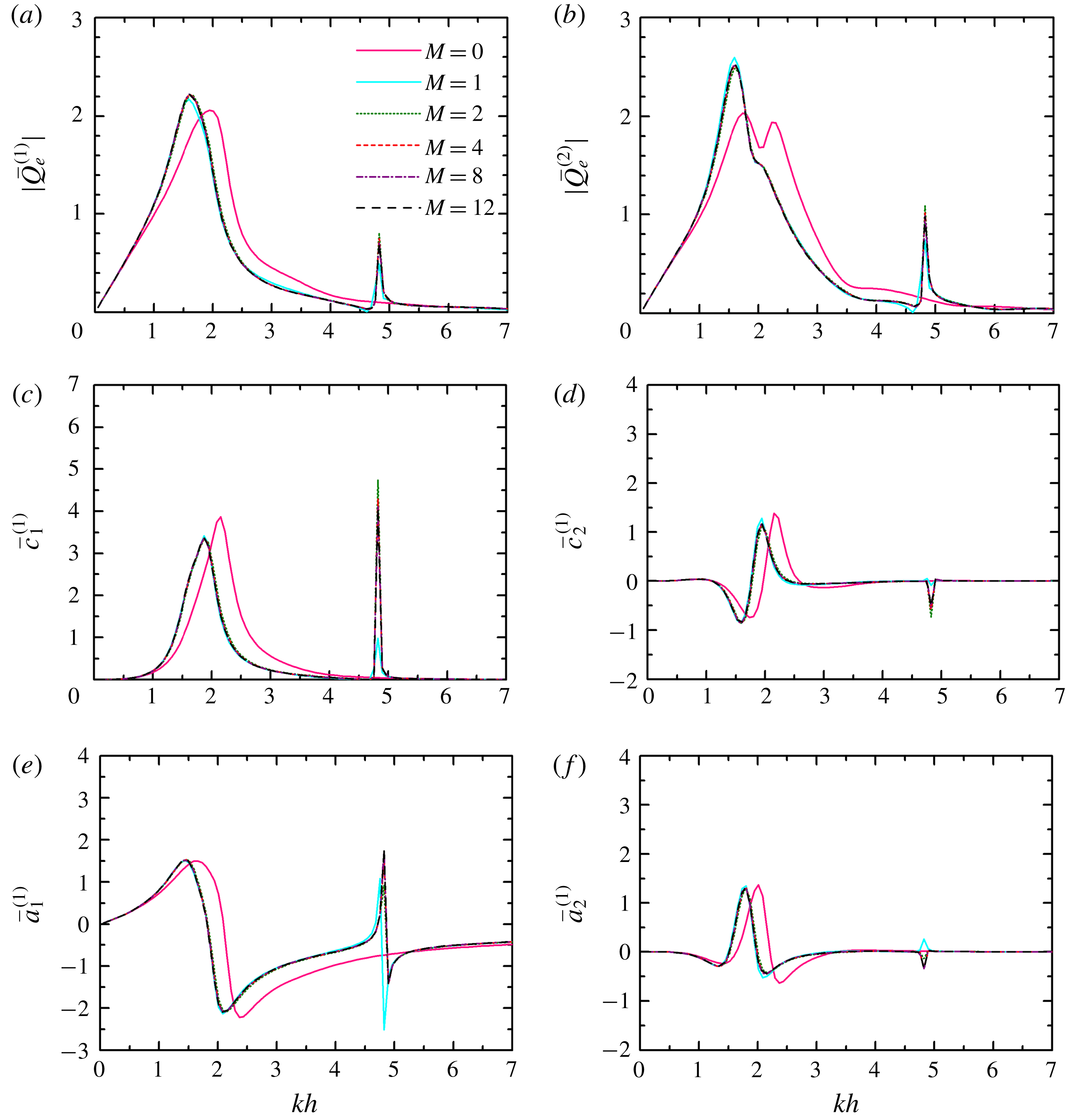
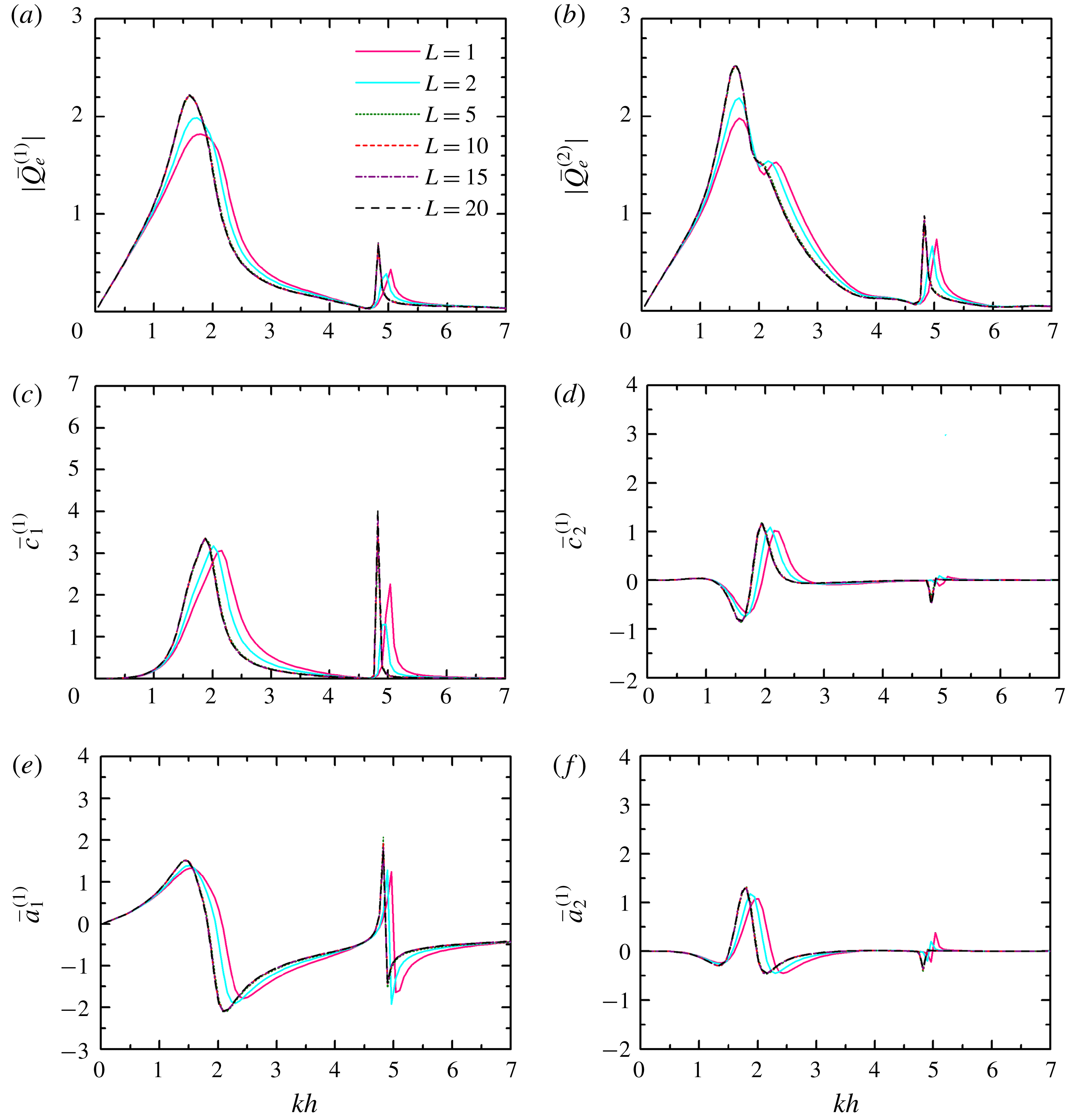
Figures 2 and 3 illustrate the impact of the angular and vertical truncated cutoffs (i.e. in terms of
 $M$
and
 $L$
), respectively, on the wave excitation volume flux and hydrodynamic coefficients for two coast-integrated OWCs with
 $R/h=0.5$
,
 $(R-R_{i})/h=0.1$
,
 $d/h=0.2$
,
 $D/h=2.0$
and
 $\unicode[STIX]{x1D6FD}=\unicode[STIX]{x03C0}/6$
. Similarly, the convergence analysis was carried out for cases with a different number of OWCs and with different OWC geometry. In order to obtain the converged results,
 $M\geqslant 8$
and
 $L\geqslant 15$
are suggested. Hereinafter,
 $M=12$
and
 $L=20$
are adopted.
Impact of the angular cutoffs (i.e. in terms of
 $M$
) on wave excitation volume flux and hydrodynamic coefficients,
 $N=2$
,
 $R/h=0.5$
,
 $(R-R_{i})/h=0.1$
,
 $d/h=0.2$
,
 $D/h=2.0$
,
 $\unicode[STIX]{x1D6FD}=\unicode[STIX]{x03C0}/6$
and
 $L=20$
: (a)
 $|\bar{Q}_{e}^{(1)}|$
; (b)
 $|\bar{Q}_{e}^{(2)}|$
; (c)
 $\bar{c}_{1}^{(1)}$
; (d)
 $\bar{c}_{2}^{(1)}$
; (e)
 $\bar{a}_{1}^{(1)}$
; and (f)
 $\bar{a}_{2}^{(1)}$
.

Impact of the vertical cutoffs (i.e. in terms of
 $L$
) on wave excitation volume flux and hydrodynamic coefficients,
 $N=2$
,
 $R/h=0.5$
,
 $(R-R_{i})/h=0.1$
,
 $d/h=0.2$
,
 $D/h=2.0$
,
 $\unicode[STIX]{x1D6FD}=\unicode[STIX]{x03C0}/6$
and
 $M=12$
: (a)
 $|\bar{Q}_{e}^{(1)}|$
; (b)
 $|\bar{Q}_{e}^{(2)}|$
; (c)
 $\bar{c}_{1}^{(1)}$
; (d)
 $\bar{c}_{2}^{(1)}$
; (e)
 $\bar{a}_{1}^{(1)}$
; and (f)
 $\bar{a}_{2}^{(1)}$
.

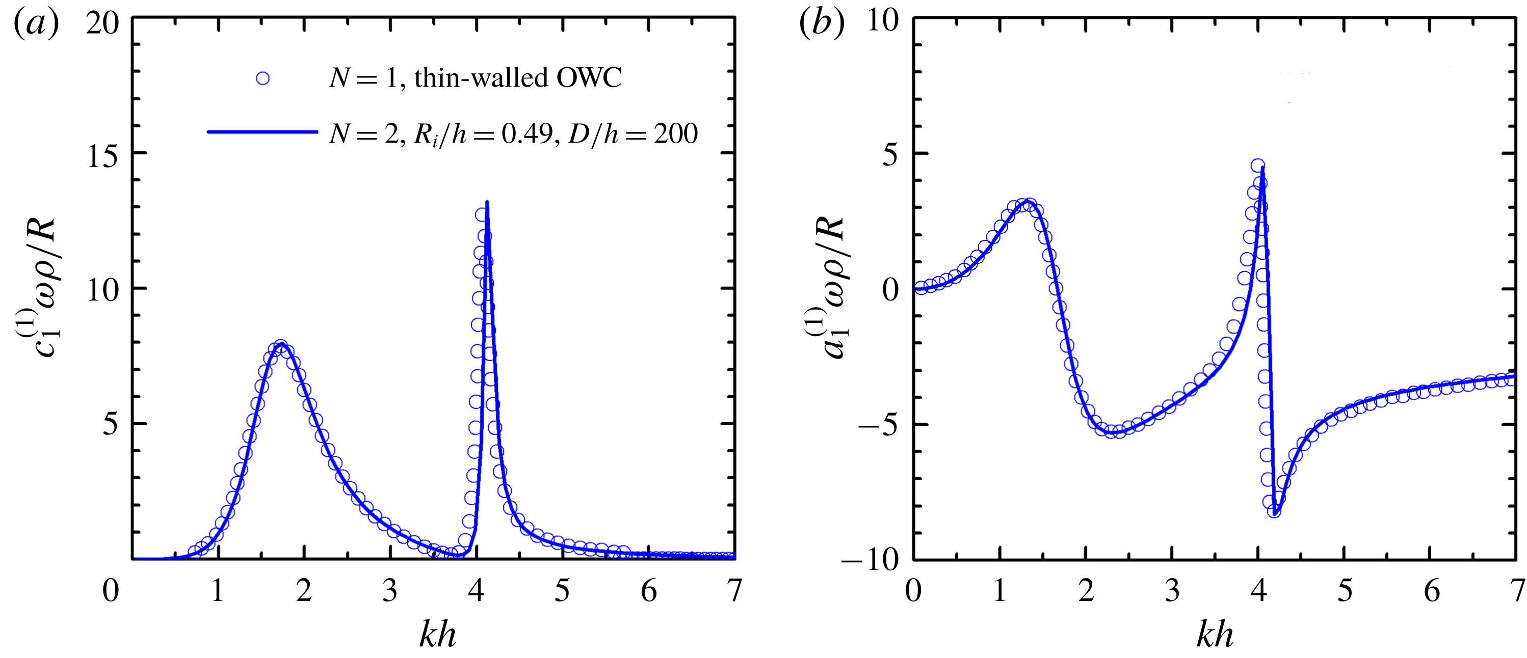
The present theoretical model is focused on an array of coast-integrated OWCs (i.e.
 $N\geqslant 2$
) without the thin-walled assumption (i.e.
 $R_{i}<R$
). By contrast, if the OWCs are deployed far away from each other and the thickness of the OWC wall tends to zero (i.e.
 $R_{i}\approx R$
), the present model could be used to solve the hydrodynamic problems from a thin-walled coast-integrated OWC (i.e.
 $R_{i}=R$
) approximately, which was investigated by Martins-Rivas & Mei (Reference Martins-Rivas and Mei2009a
). Figure 4 plots the frequency response of
 $c_{1}^{(1)}$
and
 $a_{1}^{(1)}$
of the coast-integrated OWC(s) with
 $R/h=0.5$
and
 $d/h=0.2$
. The present results with
 $N=2$
,
 $R_{i}/h=0.49$
, i.e.
 $(R-R_{i})/R=0.02$
, and
 $D/h=200$
are in good agreement with those of a single coast-integrated OWC under the thin-wall restriction (Martins-Rivas & Mei Reference Martins-Rivas and Mei2009a
).
Frequency response of
 $c_{1}^{(1)}$
and
 $a_{1}^{(1)}$
of the coast-integrated OWC(s) with
 $R/h=0.5$
and
 $d/h=0.2$
: (a)
 $c_{1}^{(1)}$
; and (b)
 $a_{1}^{(1)}$
. Circles: results from Martins-Rivas & Mei (Reference Martins-Rivas and Mei2009a
) for a thin-walled OWC, i.e.
 $R_{i}=R$
; lines: present results for two OWCs far away from each other.

Additionally, figure 5 illustrates the behaviour of
 $\bar{c}_{1}^{(1)}$
and
 $\bar{c}_{2}^{(1)}$
versus the non-dimensional wavenumber
 $kh$
for two coast-integrated OWCs with
 $R/h=0.5$
,
 $(R-R_{i})/h=0.1$
,
 $d/h=0.2$
and
 $D/h=2.0$
. The plotted results of
 $\bar{c}_{1}^{(1)}$
and
 $\bar{c}_{2}^{(1)}$
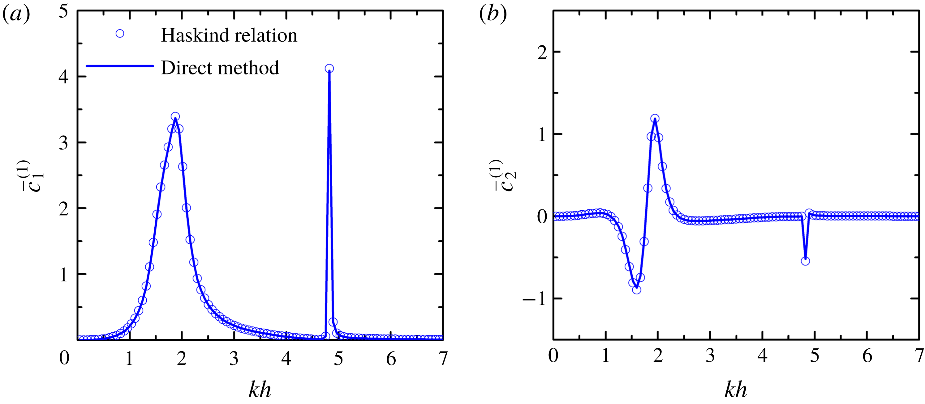
obtained using the direct method and the Haskind relation cannot be distinguished. This excellent agreement between them, together with the results in figure 4, indicate the accuracy of separate computations of scattering and radiation potentials.
Results of wave damping coefficients by using the direct method and the indirect method based on the Haskind relation,
 $N=2$
,
 $R/h=0.5$
,
 $(R-R_{i})/h=0.1$
,
 $d/h=0.2$
and
 $D/h=2.0$
: (a)
 $\bar{c}_{1}^{(1)}$
; and (b)
 $\bar{c}_{2}^{(1)}$
.

As displayed in figure 5(a), there are two peaks of
 $\bar{c}_{1}^{(1)}$
(
 $kh=1.88$
and 4.82) in the computed range of
 $kh$
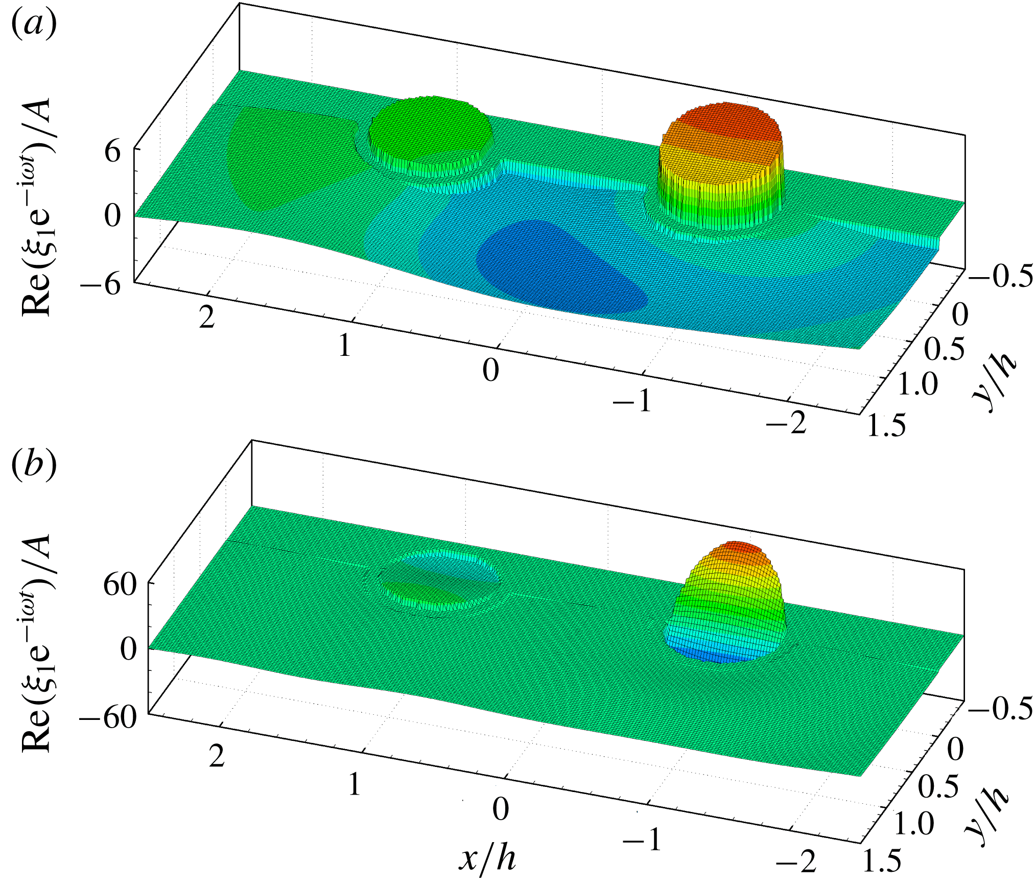
. Figure 6 presents the free-surface patterns (
 $\text{Re}(\unicode[STIX]{x1D709}_{1}\text{e}^{-\text{i}\unicode[STIX]{x1D714}t})/A=\text{Re}(\text{i}\unicode[STIX]{x1D714}p_{1}\unicode[STIX]{x1D6F7}_{1}\text{e}^{-\text{i}\unicode[STIX]{x1D714}t}/g)/A$
) in- and outside the two OWC chambers corresponding to these two peaks of
 $\bar{c}_{1}^{(1)}$
. Owing to the existence of the coast, the opening of each coast-integrated OWC is asymmetrical; as a result, in addition to the Helmholtz mode (the so-called pumping mode), another mode (i.e. the so-called sloshing mode) of the OWC is excited. As shown in figure 6(a), the pumping mode dominates the wave motion inside each OWC chamber for
 $kh=1.88$
. For
 $kh=4.82$
, as can be seen from figure 6(b), the wave motion inside the OWC chambers is dominated by the sloshing mode.
Radiation problem: free-surface elevation inside and around the coast-integrated OWCs,
 $N=2$
,
 $R/h=0.5$
,
 $(R-R_{i})/h=0.1$
,
 $d/h=0.2$
,
 $D/h=2.0$
,
 $p_{1}=\unicode[STIX]{x1D70C}gA$
and
 $p_{2}=0$
: (a)
 $kh=1.88$
at
 $t=3\unicode[STIX]{x03C0}/2\unicode[STIX]{x1D714}$
; and (b)
 $kh=4.82$
, at
 $t=\unicode[STIX]{x03C0}/2\unicode[STIX]{x1D714}$
.

As illustrated in figure 5, compared to the lower peak of
 $\bar{c}_{1}^{(1)}$
(
 $kh=1.88$
), the higher one (
 $kh=4.82$
) is sharper and much narrower. Here, as given in figure 7,
 $kh=1.88$
is taken as an example to present the scattering results of the free-surface patterns (
 $\text{Re}(\unicode[STIX]{x1D709}_{0}\text{e}^{-\text{i}\unicode[STIX]{x1D714}t})/A=\text{Re}(\text{i}\unicode[STIX]{x1D714}\unicode[STIX]{x1D6F7}_{0}\text{e}^{-\text{i}\unicode[STIX]{x1D714}t}/g)/A$
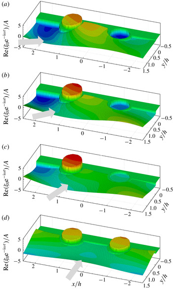
) in- and outside the OWC chambers under incident waves with different angles of incidence:
 $\unicode[STIX]{x1D6FD}=\unicode[STIX]{x03C0}/6,~\unicode[STIX]{x03C0}/4,~\unicode[STIX]{x03C0}/3$
and
 $\unicode[STIX]{x03C0}/2$
. Despite the fact that, generally speaking, the scattering wave motion around the integrated OWCs depends on the incident wave direction, the motion inside the OWC chambers is dominated by the pumping mode for
 $kh=1.88$
, regardless of the incident wave direction (figure 7). Although the sloshing mode plays a rather weak role for such a wave condition, it can still be observed from figure 7 that the symmetrical axis of that mode tends to align itself with the incident wave direction. For
 $\unicode[STIX]{x1D6FD}=\unicode[STIX]{x03C0}/2$
, as expected, the two water columns behave the same due to the symmetry of both OWC geometry and wave field.
Scattering problem: free-surface elevation inside and around the coast-integrated OWCs,
 $N=2$
,
 $R/h=0.5$
,
 $(R-R_{i})/h=0.1$
,
 $d/h=0.2$
,
 $D/h=2.0$
,
 $t=0$
and
 $kh=1.88$
: (a)
 $\unicode[STIX]{x1D6FD}=\unicode[STIX]{x03C0}/6$
; (b)
 $\unicode[STIX]{x1D6FD}=\unicode[STIX]{x03C0}/4$
; (c)
 $\unicode[STIX]{x1D6FD}=\unicode[STIX]{x03C0}/3$
; and (d)
 $\unicode[STIX]{x1D6FD}=\unicode[STIX]{x03C0}/2$
.

5.1 Comparison between multiple and single coast-integrated/offshore OWCs
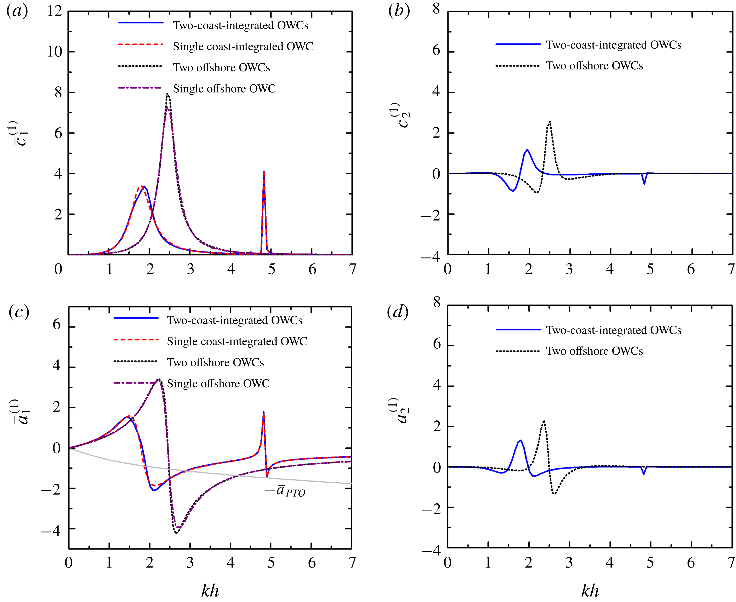
Figure 8 displays the frequency responses of the hydrodynamic coefficients for two coast-integrated OWCs, the same OWCs in the open sea and a single coast-integrated/offshore OWC (Zheng et al.
Reference Zheng, Zhang and Iglesias2018, Reference Zheng, Zhang and Iglesias2019). For all four cases in the full range of
 $kh$
,
 $\bar{c}_{1}^{(1)}$
is positive (figure 8
a), which is reasonable from the perspective of energy conservation and outgoing propagation of radiated waves (Zheng & Zhang Reference Zheng and Zhang2018). For both the single and two offshore OWC(s) cases, there is only one peak of the
 $\bar{c}_{1}^{(1)}$
–
 $kh$
curve at
 $kh=2.44$
in the computed range of
 $kh$
, which corresponds to a pumping mode. The peak value of
 $\bar{c}_{1}^{(1)}$
for the two offshore OWCs is somewhat larger than that of the single offshore OWC due to the hydrodynamic interaction between them. For the single/two coast-integrated OWC(s) cases, two modes are excited – the lower (around
 $kh=1.85$
) dominated by the pumping mode, the higher (at
 $kh=4.82$
) dominated by the sloshing mode. Owing to the constraint of the coastline, the wave motion inside the OWC chamber is more restricted compared to that of the offshore cases, leading to smaller peaks of
 $\bar{c}_{1}^{(1)}$
. As can be seen from figure 8(c), the corresponding
 $\bar{a}_{1}^{(1)}$
parameter changes its sign rapidly around those
 $kh$
values where the peaks of
 $\bar{c}_{1}^{(1)}$
occur. Since the effect of hydrostatic stiffness has already been included in
 $\bar{a}_{1}^{(1)}$
, the
 $kh$
values where
 $\bar{a}_{1}^{(1)}$
vanishes correspond to natural resonance. The light grey line plotted in figure 8(c) represents
 $-\bar{a}_{PTO}$
, which is induced by the air compressibility. When taken into account, resonance happens at the
 $kh$
values where the
 $\bar{a}_{1}^{(1)}$
and
 $-\bar{a}_{PTO}$
curves intersect each other. For the two offshore/coast-integrated OWCs (figure 8
b,d), the ranges of
 $\bar{c}_{2}^{(1)}$
and
 $\bar{a}_{2}^{(1)}$
are comparable to those of
 $\bar{c}_{1}^{(1)}$
and
 $\bar{a}_{1}^{(1)}$
, indicating the significant influence of the hydrodynamic interaction between multiple OWCs.
Radiation problem,
 $R/h=0.5$
,
 $(R-R_{i})/h=0.1$
,
 $d/h=0.2$
,
 $D/h=2.0$
and
 $h=10~\text{m}$
: (a)
 $\bar{c}_{1}^{(1)}$
; (b)
 $\bar{c}_{2}^{(1)}$
; (c)
 $\bar{a}_{1}^{(1)}$
and
 $-\bar{a}_{PTO}$
; and (d)
 $\bar{a}_{2}^{(1)}$
.

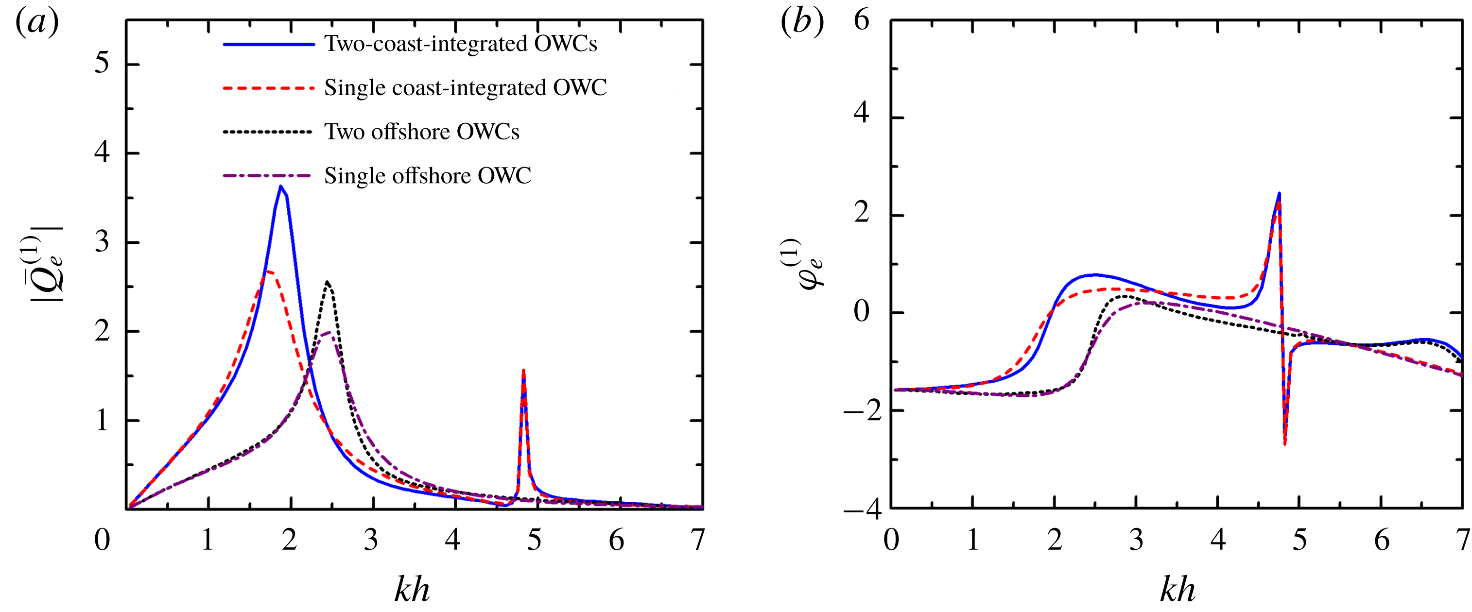
The frequency responses of the wave excitation volume flux in terms of the amplitude and phase for these four cases subjected to incident waves with
 $\unicode[STIX]{x1D6FD}=\unicode[STIX]{x03C0}/2$
are plotted in figure 9. The basic shapes of the
 $|\bar{Q}_{e}^{(1)}|$
–
 $kh$
curves (figure 9
a) look similar to those of
 $\bar{c}_{1}^{(1)}$
–
 $kh$
(figure 8
a). However, due to the wave reflection from the vertical coastline, the peaks of
 $|\bar{Q}_{e}^{(1)}|$
for the coast-integrated OWC(s) are larger than those of offshore situations, and clearly shift towards lower frequencies. The shift of the position of the peaks can be explained from the point of view of the natural modes: compared to the offshore OWC(s), for which the space under the chamber wall is entirely open to the water, in the case of the coast-integrated OWC(s), half of the space below the chamber on the coast side is closed, implying that a greater proportion of the water column is enclosed. This leads to smaller natural frequencies and, therefore, the OWC(s) are more likely to be significantly excited at lower frequencies. The peaks of
 $|\bar{Q}_{e}^{(1)}|$
for the two OWCs, regardless of whether they are coast-integrated or offshore, can benefit from the hydrodynamic interaction between them, e.g. the peak value of
 $|\bar{Q}_{e}^{(1)}|$
of 2.69 for the single coast-integrated OWC, which is reached for
 $kh=1.73$
, is enhanced to 3.64 for the two coast-integrated OWCs, and occurs at
 $kh=1.88$
. In long waves, e.g.
 $kh<1.5$
, the size of the OWCs is small compared to the wavelength, so that the primary effect on the wave field is reflection at the coast, leading to an overlapping of
 $\unicode[STIX]{x1D711}_{e}^{(1)}$
–
 $kh$
for the single/two OWC(s) cases and a separation for offshore and coast-integrated situations (figure 9
b).
Scattering problem,
 $R/h=0.5$
,
 $(R-R_{i})/h=0.1$
,
 $d/h=0.2$
,
 $D/h=2.0$
and
 $\unicode[STIX]{x1D6FD}=\unicode[STIX]{x03C0}/2$
: (a) amplitude of wave excitation volume flux,
 $|\bar{Q}_{e}^{(1)}|$
; and (b) phase of wave excitation volume flux,
 $\unicode[STIX]{x1D711}_{e}^{(1)}$
.

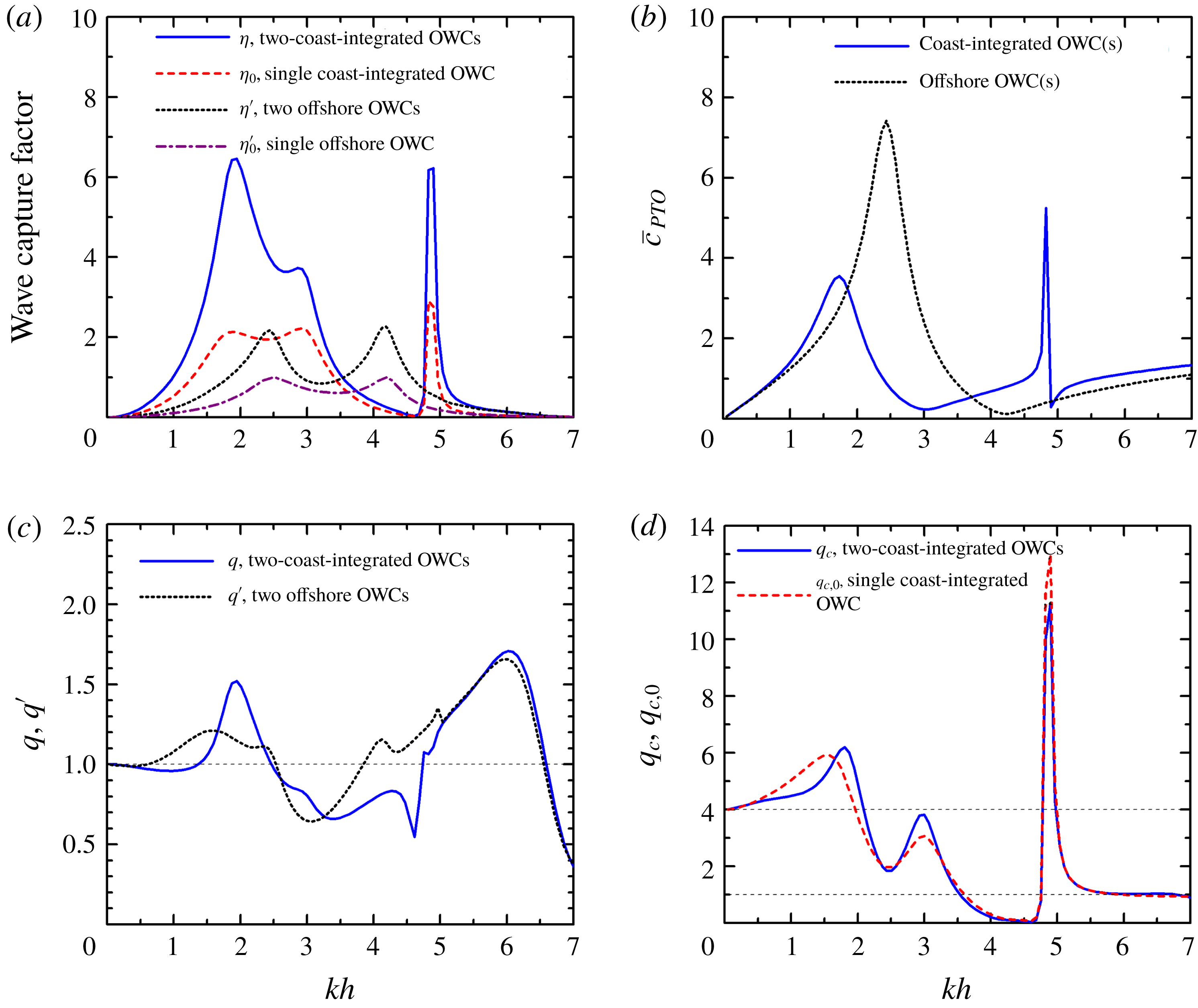
The wave power extraction from these four cases of OWC(s) are displayed in figure 10 in terms of power capture factor, array factor, coast factor and PTO damping employed. The curve of
 $-\bar{a}_{PTO}$
intersects the curve of
 $\bar{a}_{1}^{(1)}$
at two values of
 $kh$
, i.e. 2.47 and 4.19, in the computed range of
 $kh$
for single/two offshore OWC(s) (see figure 8
c), and the corresponding wave capture factors (
 $\unicode[STIX]{x1D702}^{\prime }$
and
 $\unicode[STIX]{x1D702}_{0}^{\prime }$
) as shown in figure 10(a) also attain their optimum at these two wave frequencies. The value of
 $\unicode[STIX]{x1D702}_{0}^{\prime }$
is exactly 1.0 at the resonant frequencies displayed, which is reasonable and can be theoretically derived by using the Haskind relation (e.g. Falnes Reference Falnes2002). For the two offshore OWCs case, the largest value of the wave capture factor (
 $\unicode[STIX]{x1D702}^{\prime }$
as displayed in figure 10
a) can reach 2.27. There is an obvious drop in
 $\unicode[STIX]{x1D702}^{\prime }$
between these two resonant frequencies, for
 $kh\in (3.0,3.5)$
, implying that the two OWCs cannot continuously capture wave power effectively in a large range of
 $kh$
. When the OWC(s) is(are) integrated into a coast, three intersections of
 $\bar{a}_{1}^{(1)}$
and
 $-\bar{a}_{PTO}$
occur, at
 $kh=1.88$
, 2.92 and 4.82 (figure 8
c), resulting in three peaks of
 $\unicode[STIX]{x1D702}$
and
 $\unicode[STIX]{x1D702}_{0}$
(figure 10
a). Compared to those of the offshore cases, although the first two resonant frequencies of the coast-integrated cases are closer to each other,
 $\unicode[STIX]{x1D702}_{0}$
remains mostly around 2.0 for
 $kh$
between these two frequencies, leading to an even broader bandwidth of high efficiency. For the two coast-integrated OWCs, thanks to the constructive hydrodynamic interaction between them, a large peak value of
 $\unicode[STIX]{x1D702}$
, 6.46, is achieved around
 $kh=1.88$
. The corresponding
 $\bar{c}_{PTO}$
(figure 10
b) shows that, in order to reach optimum efficiency for all wave conditions, the turbine parameter for the coast-integrated cases does not need to be varied as much as that in the offshore cases, making it relatively easy to achieve in practice.
Power extraction,
 $R/h=0.5$
,
 $(R-R_{i})/h=0.1$
,
 $d/h=0.2$
,
 $D/h=2.0$
,
 $\unicode[STIX]{x1D6FD}=\unicode[STIX]{x03C0}/2$
and
 $h=10~\text{m}$
: (a) wave capture factor,
 $\unicode[STIX]{x1D702}$
,
 $\unicode[STIX]{x1D702}_{0}$
,
 $\unicode[STIX]{x1D702}^{\prime }$
and
 $\unicode[STIX]{x1D702}_{0}^{\prime }$
; (b)
 $\bar{c}_{PTO}$
; (c) array factor,
 $q$
and
 $q^{\prime }$
; and (d) coast factor,
 $q_{c}$
and
 $q_{c,0}$
.

The variation of the array factor for the coast-integrated and offshore cases (i.e.
 $q$
and
 $q^{\prime }$
) with
 $kh$
(figure 10
c) indicates that both
 $q$
and
 $q^{\prime }$
tend to unity as
 $kh$
tends to 0. As a comparison, the coast reflection effect factor for single/two coast-integrated cases (i.e.
 $q_{c}$
and
 $q_{c,0}$
, figure 10
d) tends to 4.0 when
 $kh$
tends to 0. This is due to the fact that incident waves are the dominant element in the excitation volume flux under long waves. In the open sea, the amplitude of undisturbed incident waves is
 $A$
, whereas the amplitude of incident waves subjected to reflection from the vertical coast turns out to be
 $2A$
, leading to a doubling of the excitation volume flux and, in turn, affecting wave power extraction. For short waves, e.g.
 $kh>5.5$
, the curves of
 $q$
and
 $q^{\prime }$
tend to overlap each other and the values of
 $q_{c}$
and
 $q_{c,0}$
both approach unity. This can be explained by the dominant role of
 $\bar{c}_{PTO}$
and
 $\bar{a}_{PTO}$
in the wave power capture factor (refer to (4.5)) in short wave conditions. For
 $kh>6.0$
, all hydrodynamic coefficients vanish alongside the wave excitation volume flux (figures 8–10), whereas
 $\bar{c}_{PTO}$
and
 $\bar{a}_{PTO}$
remain non-vanishing and become even larger with the increase of
 $kh$
. As displayed in figure 10(d), for most wave conditions, except
 $kh\in (3.5,4.8)$
and
 $kh>5.5$
, the coast factors remain far above unity, indicating a constructive effect of coast reflection on wave power absorption. However, the array factor oscillates around 1.0 and shows alternating constructive and destructive effects with the change of
 $kh$
(figure 10
c). In the following sections, only the wave capture factor and array factor are preserved to indicate power extraction of the coast-integrated OWCs. As can be seen from figure 10(a,c,d), the dramatic peak of
 $\unicode[STIX]{x1D702}$
occurring at
 $kh=1.88$
benefits from both the constructive array effect (
 $q=1.5$
) and the constructive coast effect (
 $q_{c}=6.0$
).
5.2 Effect of incident wave direction
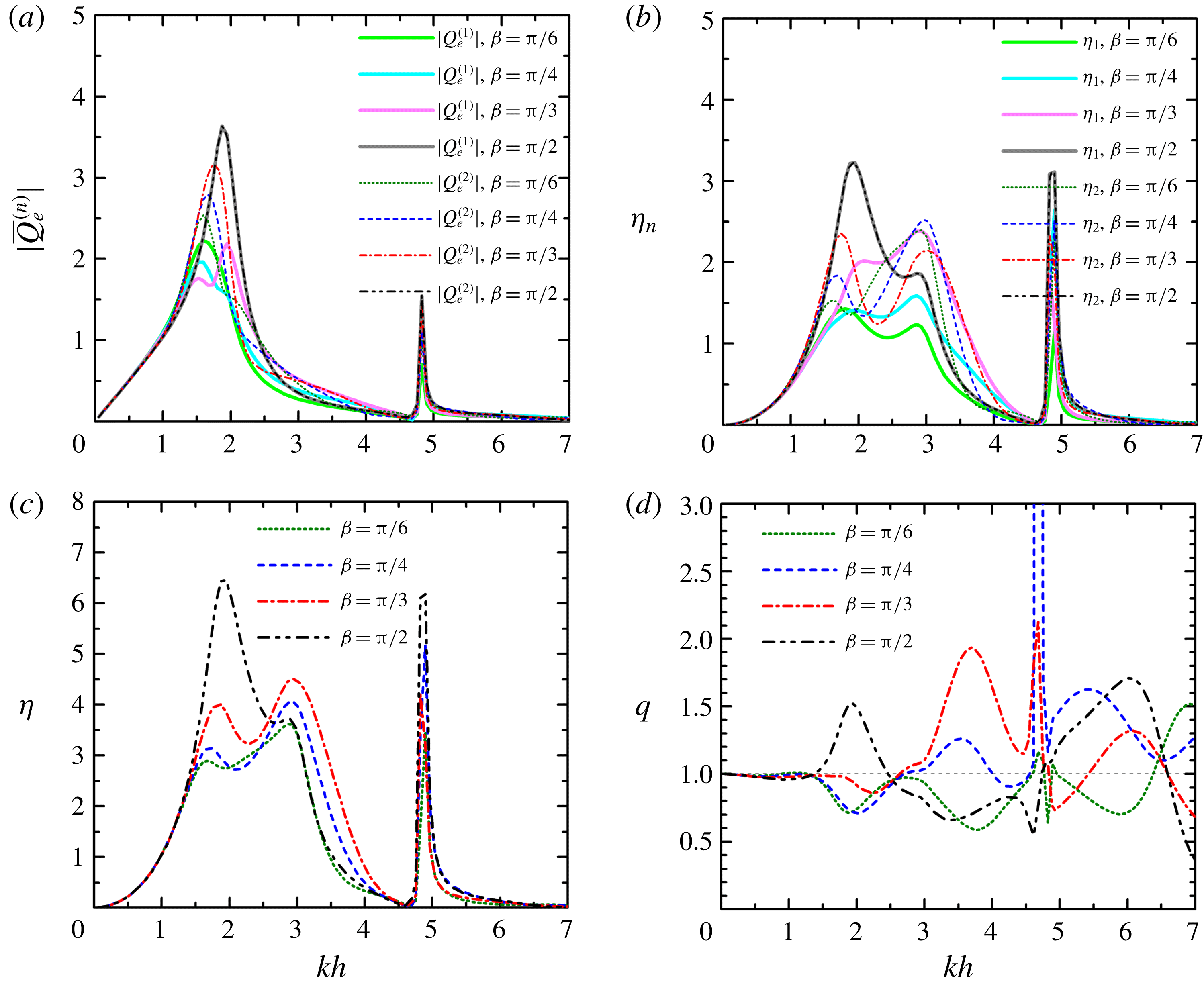
The wave excitation volume flux of each OWC, the power capture factor of each OWC and both together with the
 $q$
-factor for different incident wave directions
 $\unicode[STIX]{x1D6FD}$
are displayed in figure 11. As
 $\unicode[STIX]{x1D6FD}$
increases from
 $\unicode[STIX]{x03C0}/6$
to
 $\unicode[STIX]{x03C0}/2$
, the main peak of the wave excitation volume flux of the up-wave OWC (
 $|\bar{Q}_{e}^{(2)}|$
) becomes larger and shifts towards large
 $kh$
. The first peak for the other OWC (
 $|\bar{Q}_{e}^{(1)}|$
), on the contrary, first falls and shifts towards small
 $kh$
, and then rises and shifts in the opposite direction rapidly to the same position of
 $|\bar{Q}_{e}^{(2)}|$
for
 $\unicode[STIX]{x1D6FD}=\unicode[STIX]{x03C0}/2$
. Note that, at
 $kh\approx 2.0$
, a slight rise of the
 $|\bar{Q}_{e}^{(1)}|$
or
 $|\bar{Q}_{e}^{(2)}|$
curves with specified values of
 $\unicode[STIX]{x1D6FD}$
is observed, e.g. more particularly, an additional peak of the
 $|\bar{Q}_{e}^{(1)}|$
–
 $kh$
curve for
 $\unicode[STIX]{x1D6FD}=\unicode[STIX]{x03C0}/3$
can be excited. This appears to be induced by the resonance of water waves between the two OWCs, for
 $k(D-R)\approx \unicode[STIX]{x03C0}$
is satisfied for these cases at
 $kh\approx 2.0$
. For
 $\unicode[STIX]{x1D6FD}=\unicode[STIX]{x03C0}/6$
and
 $\unicode[STIX]{x03C0}/4$
, the wave power capture factor of the up-wave OWC (
 $\unicode[STIX]{x1D702}_{2}$
) is generally larger than the down-wave one (
 $\unicode[STIX]{x1D702}_{1}$
) for
 $kh\in (1.5,3.5)$
(figure 11
b), whereas for
 $\unicode[STIX]{x1D6FD}=\unicode[STIX]{x03C0}/3$
,
 $\unicode[STIX]{x1D702}_{1}>\unicode[STIX]{x1D702}_{2}$
is observed for
 $kh\in (2.0,3.0)$
. As displayed in figure 11(c), for
 $kh\in (1.5,2.0)$
, the overall power capture factor (
 $\unicode[STIX]{x1D702}$
) increases dramatically with the increase of
 $\unicode[STIX]{x1D6FD}$
from
 $\unicode[STIX]{x03C0}/6$
to
 $\unicode[STIX]{x03C0}/2$
. For
 $kh\in (2.6,4.0)$
, the
 $\unicode[STIX]{x1D702}$
corresponding to
 $\unicode[STIX]{x1D6FD}=\unicode[STIX]{x03C0}/3$
is significantly greater than those for all three other incident wave directions, including
 $\unicode[STIX]{x1D6FD}=\unicode[STIX]{x03C0}/2$
. This can be explained from the perspective of the array effect as illustrated in figure 11(d), in which constructive (
 $q>1.0$
) and destructive (
 $q<1.0$
) effects are indicated for
 $\unicode[STIX]{x1D6FD}=\unicode[STIX]{x03C0}/3$
and
 $\unicode[STIX]{x03C0}/2$
, respectively, for
 $kh\in (2.6,4.0)$
. The following sections focus on the cases with
 $\unicode[STIX]{x1D6FD}=\unicode[STIX]{x03C0}/2$
.
Comparison for different incident direction,
 $\unicode[STIX]{x1D6FD}$
, with
 $N=2$
,
 $R/h=0.5$
,
 $(R-R_{i})/h=0.1$
,
 $d/h=0.2$
,
 $D/h=2.0$
and
 $h=10~\text{m}$
: (a)
 $|\bar{Q}_{e}^{(n)}|$
; (b)
 $\unicode[STIX]{x1D702}_{n}$
; (c)
 $\unicode[STIX]{x1D702}$
; and (d)
 $q$
-factor.

Note that, at
 $kh=1.88$
, the maximum
 $\unicode[STIX]{x1D702}$
for
 $\unicode[STIX]{x1D6FD}=\unicode[STIX]{x03C0}/2$
is dramatically higher than 4.0, while the
 $\unicode[STIX]{x1D702}$
values for
 $\unicode[STIX]{x1D6FD}=\unicode[STIX]{x03C0}/6$
and
 $\unicode[STIX]{x03C0}/4$
are obviously lower than 4.0. Instead, at
 $kh=2.92$
, the
 $\unicode[STIX]{x1D702}$
values for the four cases with different values of
 $\unicode[STIX]{x1D6FD}$
are all concentrated around 4.0. In fact, for any certain wave frequency, there is a general identity of the optimum wave capture factor (
 $\unicode[STIX]{x1D702}_{MAX}$
) over all incidence angles that multiple coast-integrated OWCs must hold regardless of the OWC dimension, i.e.
 $$\begin{eqnarray}\frac{1}{\unicode[STIX]{x03C0}}\int _{0}^{\unicode[STIX]{x03C0}}\unicode[STIX]{x1D702}_{MAX}(\unicode[STIX]{x1D6FD})\hspace{2.22198pt}\text{d}\unicode[STIX]{x1D6FD}=2N,\end{eqnarray}$$
which can be theoretically confirmed by invoking the ideal optimization criteria and the Haskind relation (Wolgamot, Taylor & Taylor Reference Wolgamot, Taylor and Taylor2012). A detailed derivation is given in appendix B.
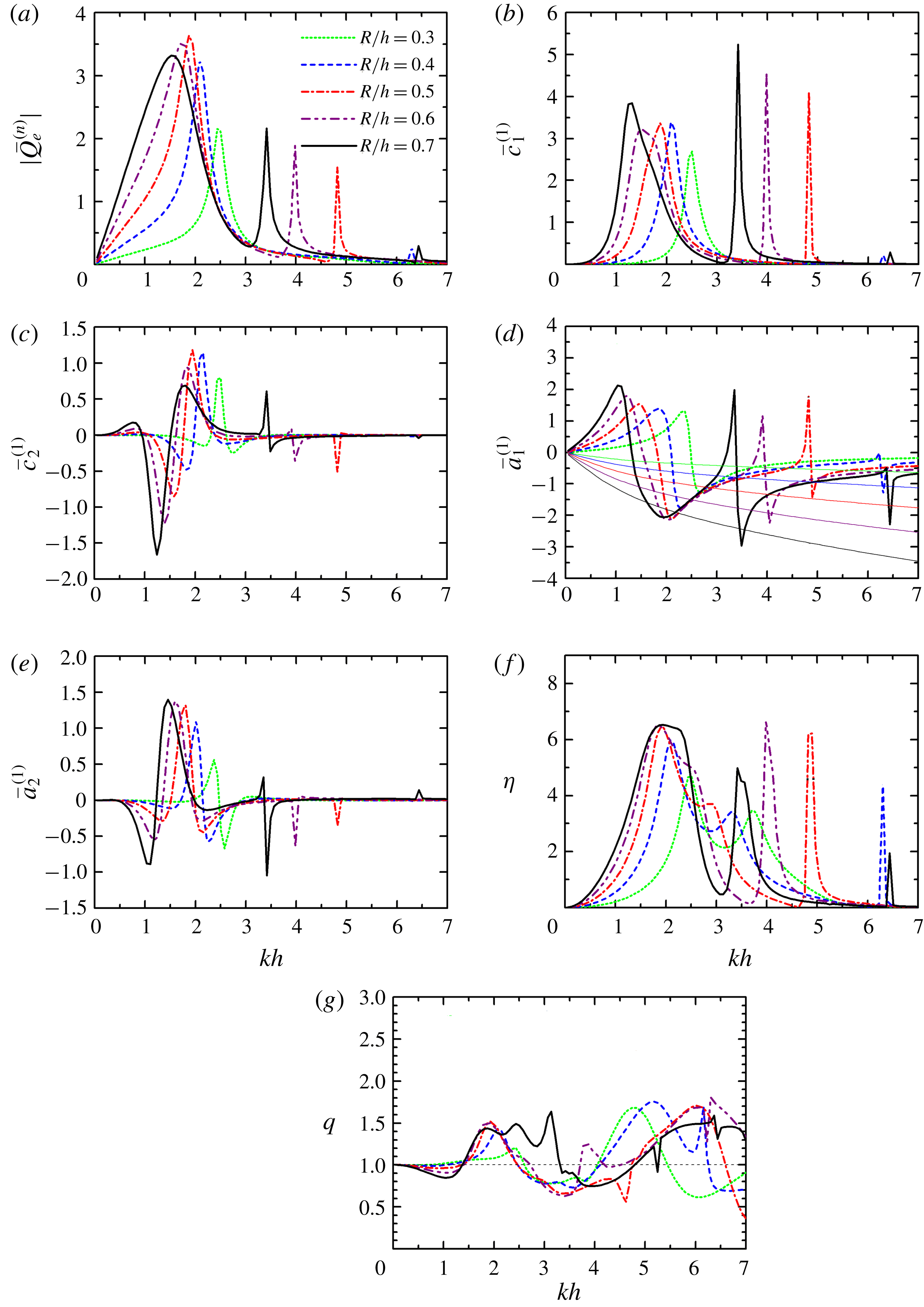
Comparison for different radius of the OWCs,
 $R/h$
, with
 $N=2$
,
 $(R-R_{i})/h=0.1$
,
 $d/h=0.2$
,
 $D/h=2.0$
,
 $\unicode[STIX]{x1D6FD}=\unicode[STIX]{x03C0}/2$
and
 $h=10~\text{m}$
: (a)
 $|\bar{Q}_{e}^{(n)}|$
; (b)
 $\bar{c}_{1}^{(1)}$
; (c)
 $\bar{c}_{2}^{(1)}$
; (d)
 $\bar{a}_{1}^{(1)}$
and
 $-\bar{a}_{PTO}$
(solid thin curves in the same colour of
 $\bar{a}_{1}^{(1)}$
for the same value of
 $R/h$
); (e)
 $\bar{a}_{2}^{(1)}$
; (f)
 $\unicode[STIX]{x1D702}$
; and (g)
 $q$
-factor.

5.3 Effect of radius of the OWCs
The effect of radius (
 $R/h$
) of the OWCs on wave excitation volume flux, hydrodynamic coefficients, wave capture factor and array factor were investigated (figure 12). As
 $R/h$
increases from 0.3 to 0.7, the main peak of the
 $|\bar{Q}_{e}^{(n)}|$
curve, as shown in figure 12(a), shifts towards lower frequencies and tends to be flatter. The peak value first becomes larger and then smaller after reaching the largest value with
 $R/h=0.5$
. As illustrated in figure 12(b), for the smallest column
 $R/h=0.3$
, the curve of
 $\bar{c}_{1}^{(1)}$
has only one peak in the computed range of
 $kh$
. For larger
 $R/h$
, i.e.
 $R/h=0.4{-}0.6$
and
 $R/h=0.7$
, two and three peaks, are evident, respectively. This is associated with the natural resonance modes (without PTO system), which are strongly dependent on the relative size of OWC chamber to wavelength. Figure 12(c,e) indicates that, with the increase of
 $R/h$
, the oscillation amplitudes of the
 $\bar{c}_{2}^{(1)}$
and
 $\bar{a}_{2}^{(1)}$
curves become larger, and the
 $kh$
corresponding to these largest amplitudes get smaller. As previously defined in § 4,
 $\bar{a}_{PTO}$
depends on the chamber volume
 $V_{0}=\unicode[STIX]{x03C0}R^{2}h$
, which in turn depends critically on
 $R/h$
.
In figure 12(d), apart from the five curves of
 $\bar{a}_{1}^{(1)}$
, five solid thin curves of
 $-\bar{a}_{PTO}$
relating to five different values of
 $R/h$
are plotted in the corresponding colour. For
 $R/h=0.3$
, there are two points of interaction between
 $-\bar{a}_{PTO}$
and
 $\bar{a}_{1}^{(1)}$
in the range of
 $kh$
plotted; while for larger
 $R/h$
, more points of interaction can be achieved, e.g. four interaction points for
 $R/h=0.7$
. As
 $R/h$
increases from 0.3 to 0.7, the curve of
 $-\bar{a}_{PTO}$
is slanted downwards, resulting in the first two points of interaction moving towards lower frequencies and the horizontal distance between them getting smaller. The
 $kh$
values corresponding to the points of interaction between
 $-\bar{a}_{PTO}$
and
 $\bar{a}_{1}^{(1)}$
identified from figure 12(d) coincide well with the peak positions of the
 $\unicode[STIX]{x1D702}$
curves (figure 12
f). As
 $R/h$
increases, the main peaks of the
 $\unicode[STIX]{x1D702}$
curve shift towards lower
 $kh$
and gain intensity. Figure 12(g) shows that the
 $q$
-factor remains above unity for
 $kh\in (1.4,2.5)$
regardless of the value of
 $R/h$
. For
 $R/h=0.7$
, constructive array effects can be obtained for a rather large range of
 $kh$
, i.e.
 $kh\in (1.4,3.3)$
. Although some higher and broader peaks of
 $q$
can be achieved for
 $kh>4.5$
, they are not attractive, because either
 $\unicode[STIX]{x1D702}$
is too small, or
 $\unicode[STIX]{x1D702}$
is only large in a narrow bandwidth.
5.4 Effect of wall thickness of the OWCs
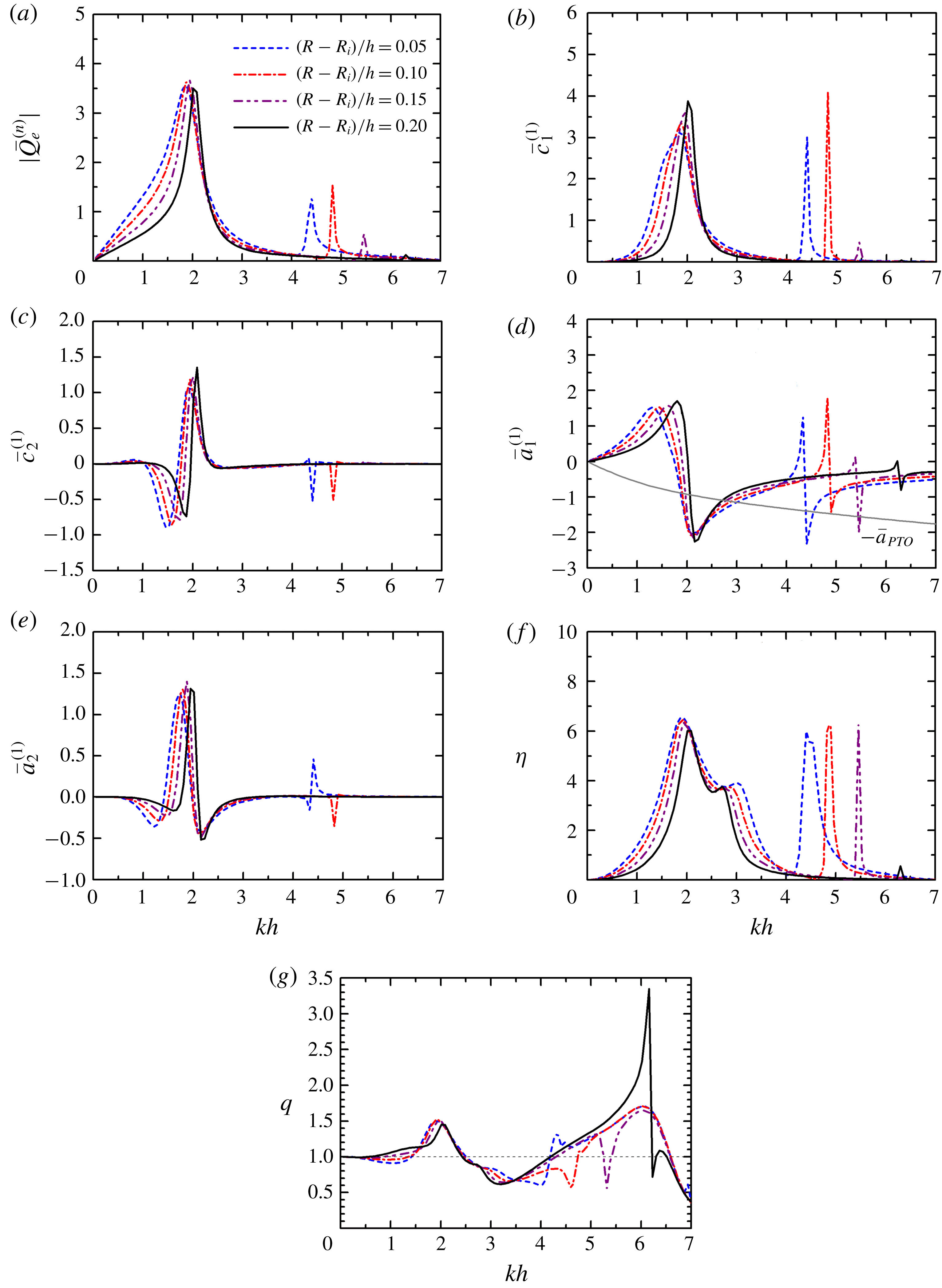
The theoretical results for the OWCs with different chamber wall thickness are plotted in figure 13. As the wall thickness of the OWC chambers increases, i.e. the inner radius of the chamber decreases while the outer radius remains constant, the main peak of
 $|\bar{Q}_{e}^{(n)}|$
shifts slightly towards higher wave frequencies with a narrower bandwidth (figure 13
a), while its peak height remains approximately the same. A similar change occurs for
 $\bar{c}_{1}^{(1)}$
(figure 13
b), with the main peak becoming higher and more abrupt with the increase of wall thickness of the OWCs. Correspondingly, the first sign changing point of
 $\bar{a}_{1}^{(1)}$
(figure 13
d) occurs at a lower frequency, and its variation in amplitude gets larger, and happens in a narrower range of
 $kh$
. With the increase of wall thickness, the position of the largest oscillation amplitude of
 $\bar{c}_{2}^{(1)}$
and
 $\bar{a}_{2}^{(1)}$
(figure 13
c,e) moves towards large
 $kh$
and the variation becomes more abrupt as well. As illustrated in figure 13(f), the peaks of
 $\unicode[STIX]{x1D702}$
at
 $kh\in (1.0,3.5)$
are lower and the overall bandwidth is narrower for a thicker wall of each OWC chamber. This can also be reflected by the intersections between the
 $-\bar{a}_{PTO}$
and
 $\bar{a}_{1}^{(1)}$
curves (figure 13
d), which get closer to each other horizontally. In figure 13(g), a smaller
 $q$
-factor is shown to be obtained for the OWCs with a thicker chamber wall for most
 $kh\in (1.8,3.5)$
, suggesting a relatively more destructive array effect. Hence it may be concluded that, to achieve higher wave power absorption efficiency in a broader bandwidth, the OWC chambers with a thinner wall are more appropriate. It should be noted that in practice the chamber wall should not be so thin as to lose structural robustness.
Comparison for different wall thickness of the OWCs,
 $(R-R_{i})/h$
, with
 $N=2$
,
 $R/h=0.5$
,
 $d/h=0.2$
,
 $D/h=2.0$
,
 $\unicode[STIX]{x1D6FD}=\unicode[STIX]{x03C0}/2$
and
 $h=10~\text{m}$
: (a)
 $|\bar{Q}_{e}^{(n)}|$
; (b)
 $\bar{c}_{1}^{(1)}$
; (c)
 $\bar{c}_{2}^{(1)}$
; (d)
 $\bar{a}_{1}^{(1)}$
and
 $-\bar{a}_{PTO}$
; (e)
 $\bar{a}_{2}^{(1)}$
; (f)
 $\unicode[STIX]{x1D702}$
; and (g)
 $q$
-factor.

5.5 Effect of submergence of the OWCs
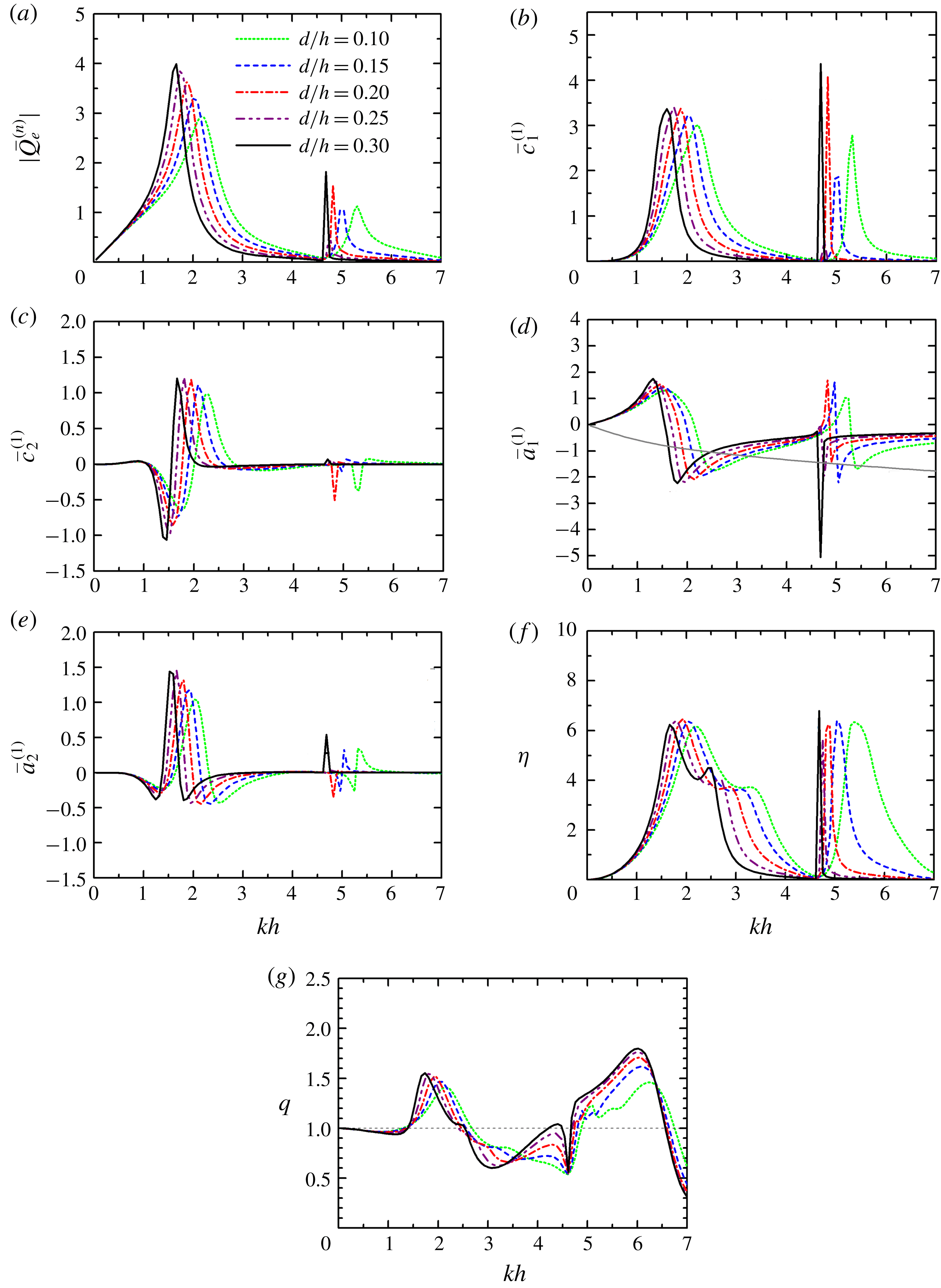
The submergence of the chamber,
 $d/h$
, can also strongly affect the hydrodynamics and power extraction of the coast-integrated OWCs. As indicated in figure 14(b,d), the peaks of
 $\bar{c}_{1}^{(1)}$
and the sign changing points of
 $\bar{a}_{1}^{(1)}$
are found to shift towards lower
 $kh$
with the increase of
 $d/h$
. This is reasonable, since a larger
 $d/h$
means a higher, heavier water column enclosed within the chamber, leading to a smaller natural frequency. As
 $d/h$
increases, the curve of
 $|\bar{Q}_{e}^{(n)}|$
becomes more abrupt (figure 14
a), and the peaks become higher and move towards low
 $kh$
. As indicated in figure 14(c,e), the frequencies corresponding to the dramatic variations of
 $\bar{c}_{2}^{(1)}$
and
 $\bar{a}_{2}^{(1)}$
decrease with increasing
 $d/h$
. It is worth noting that, with the decrease of
 $d/h$
, although the peaks of the
 $\unicode[STIX]{x1D702}$
curve remain at approximately the same levels (figure 14
f), there is a distinct movement of these peaks towards large
 $kh$
, which can be indicated as well from the position changes of the intersections between the
 $-\bar{a}_{PTO}$
and
 $\bar{a}_{1}^{(1)}$
curves (figure 14
d). Furthermore, broader and smoother peaks of
 $\unicode[STIX]{x1D702}$
are achieved for a smaller
 $d/h$
as shown in figure 14(f). For short waves, e.g.
 $kh\in (5.5,7.0)$
, more power can be captured with the decrease of
 $d/h$
, and this constructive effect becomes stronger and stronger. This is due to the fact that most wave power (approximately
 $95\,\%$
) is concentrated at no more than one-quarter of a wavelength below the still-water level, where the kinetic energy at a shallower position is more intensive compared to that at a deeper position. For most wave conditions at
 $kh\in (2.2,3.6)$
, a larger
 $q$
-factor is obtained for a smaller
 $d/h$
(figure 14
g). Therefore, to have a better array effect and ultimately to achieve high power absorption in a rather broader bandwidth, the submergence of the OWC chambers should be as small as possible. However, the realistic chamber submergence cannot be too small, otherwise the opening may not be continuously submerged in the water when the OWCs are subjected to either strong waves or a large tidal range.
Comparison for different submergence of the OWCs,
 $d/h$
, with
 $N=2$
,
 $R/h=0.5$
,
 $(R-R_{i})/h=0.1$
,
 $D/h=2.0$
,
 $\unicode[STIX]{x1D6FD}=\unicode[STIX]{x03C0}/2$
and
 $h=10~\text{m}$
: (a)
 $|\bar{Q}_{e}^{(n)}|$
; (b)
 $\bar{c}_{1}^{(1)}$
; (c)
 $\bar{c}_{2}^{(1)}$
; (d)
 $\bar{a}_{1}^{(1)}$
and
 $-\bar{a}_{PTO}$
; (e)
 $\bar{a}_{2}^{(1)}$
; (f)
 $\unicode[STIX]{x1D702}$
; and (g)
 $q$
-factor.

5.6 Effect of distance between the OWCs
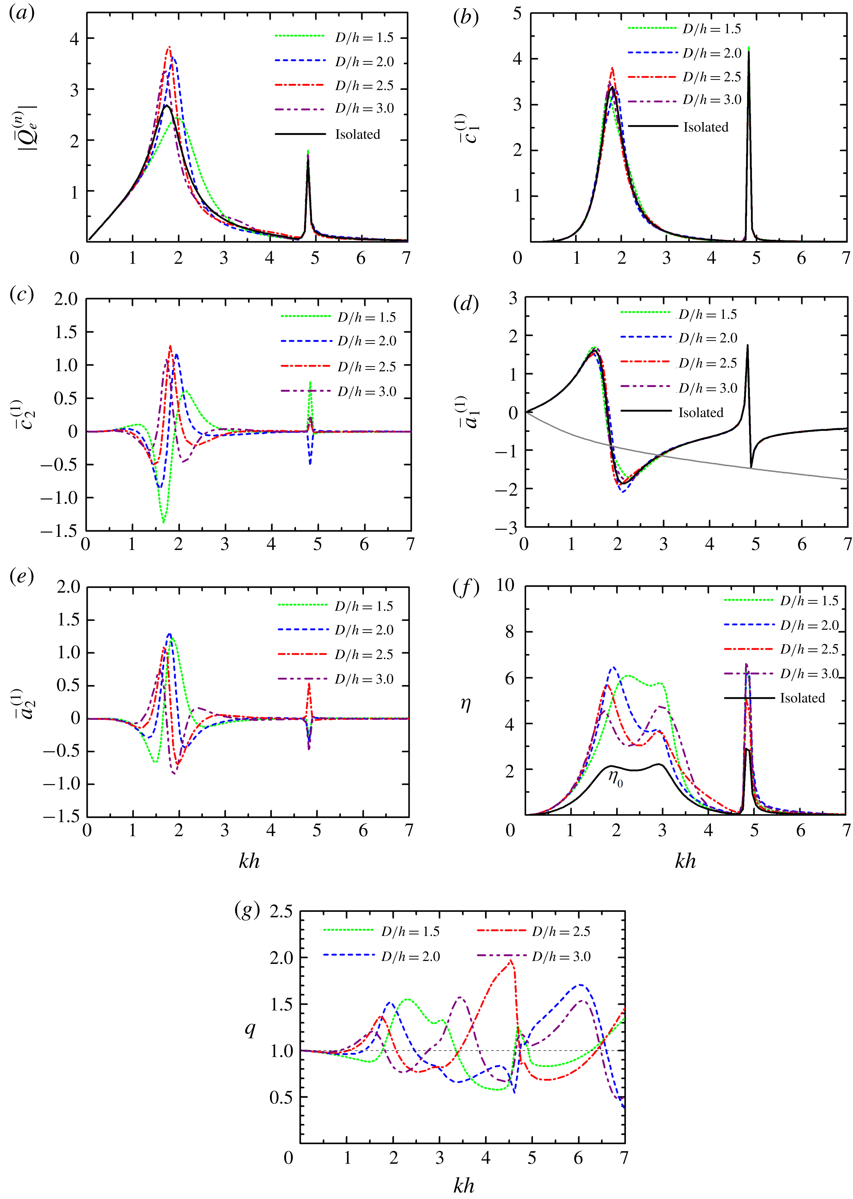
Figure 15 presents the effect of distance between the OWCs. Similar results for the individually isolated single coast/breakwater-integrated OWC (denoted as ‘isolated’) are also displayed for comparison. Figure 15(a) shows that there are two peaks of the
 $|\bar{Q}_{e}^{(n)}|$
–
 $kh$
curve over the computed range of
 $kh$
, with the main one around
 $kh\approx 1.8$
and the second sharp one at a higher frequency, i.e.
 $kh\approx 4.82$
. As
 $D/h$
increases from 1.5 to 3.0, the amplitude of the main peak first increases and then decreases. Although the amplitude of the main peak for
 $D/h=1.5$
is merely 2.4, large values of
 $|\bar{Q}_{e}^{(n)}|$
compared to the other cases are obtained at
 $kh\in (2.1,3.0)$
. The
 $kh$
corresponding to the main peak shifts towards lower frequencies. The second sharp peak is nearly independent of
 $D/h$
. As shown in figure 15(b,d), a rather limited impact of
 $D/h$
on
 $\bar{c}_{1}^{(1)}$
and
 $\bar{a}_{1}^{(1)}$
is observed at
 $kh\in (1.5,2.5)$
, where the main peak of the
 $\bar{c}_{1}^{(1)}$
–
 $kh$
curve and the corresponding drop of
 $\bar{a}_{1}^{(1)}$
occur. As
 $D/h$
varies, the
 $\bar{c}_{1}^{(1)}(\bar{a}_{1}^{(1)})$
–
 $kh$
curve of the two OWCs oscillates slightly around that of the ‘isolated’ case. This is due to the fact that the waves radiated from each coast/breakwater-integrated OWC, and also those waves diffracted from the other OWC, act on the OWC in question simultaneously. The change in
 $D/h$
leads to alteration of the phase difference between the two-OWCs mutual radiated and diffracted waves, resulting in the switch of reinforcing and diminishing influences. The amplitudes of the peak of
 $\bar{c}_{1}^{(1)}$
and the drop of
 $\bar{a}_{1}^{(1)}$
at
 $kh=1.8$
are both approximately 3.5.
As a comparison (figure 15
c,e), the variations of
 $\bar{c}_{2}^{(1)}$
and
 $\bar{a}_{2}^{(1)}$
, especially for
 $kh\in (1.0,3.0)$
, are significantly dependent upon
 $D/h$
. The amplitudes of the drops of
 $\bar{c}_{2}^{(1)}$
and
 $\bar{a}_{2}^{(1)}$
around
 $kh=1.8$
are both found to be no smaller than 1.6, revealing a strong hydrodynamic interaction between the OWCs for the four cases of
 $D/h$
examined. As
 $D/h$
increases from 1.5 to 3.0, these drops of
 $\bar{c}_{2}^{(1)}$
and
 $\bar{a}_{2}^{(1)}$
become progressively weaker, and it can be expected that, for
 $D/h\rightarrow \infty$
,
 $\bar{c}_{2}^{(1)}\approx 0$
and
 $\bar{a}_{2}^{(1)}\approx 0$
will be obtained. The wave power capture factor of the ‘isolated’ case, i.e.
 $\unicode[STIX]{x1D702}_{0}$
, is no more than 2.0 (figure 15
f). However, for the cases consisting of two OWCs, the value of
 $\unicode[STIX]{x1D702}>6.0$
can be obtained for certain values of
 $D/h$
due to hydrodynamic interactions. From the perspective of the peak value of
 $\unicode[STIX]{x1D702}$
, the OWCs with
 $D/h=2.0$
could be the best solution for power absorption. However, in practice, the OWCs with
 $D/h=1.5$
might be a better choice for their good performance over a broader bandwidth, with a sufficiently large wave capture factor. It can be learned (figure 15
g) that, indeed, the
 $D/h$
ratio has a strong effect on the shape of the
 $q$
-factor curve as well as on its amplitude. For
 $D/h=1.5$
,
 $q>1.0$
is satisfied at
 $kh\in (1.8,3.4)$
, meaning that a constructive hydrodynamic interaction between the OWCs is achieved in a large range of wave conditions.
Comparison for different spacing distance between the OWCs,
 $D/h$
, with
 $N=2$
,
 $R/h=0.5$
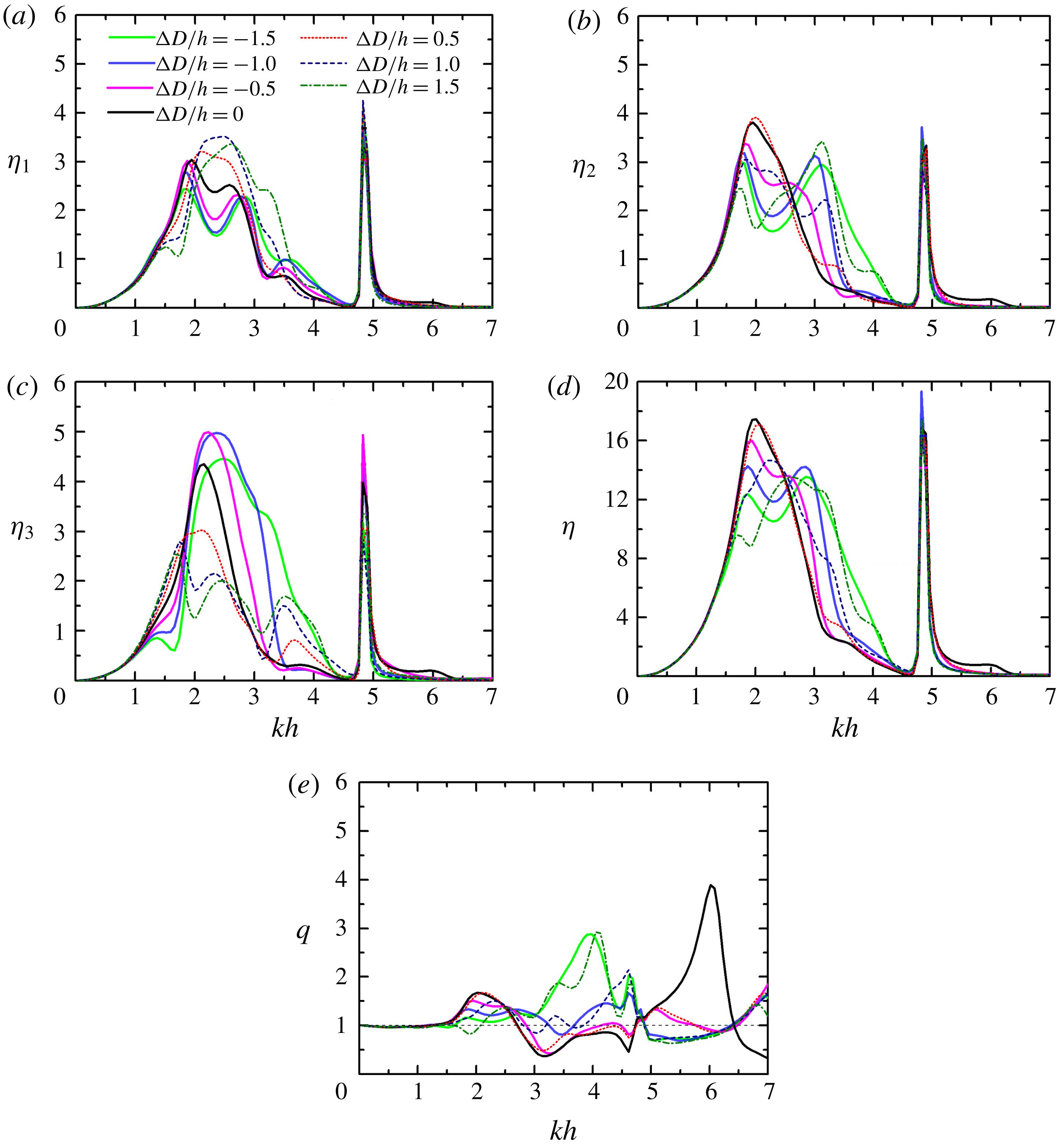
,
 $(R-R_{i})/h=0.1$
,
 $d/h=0.2$
,
 $\unicode[STIX]{x1D6FD}=\unicode[STIX]{x03C0}/2$
and
 $h=10~\text{m}$
: (a)
 $|\bar{Q}_{e}^{(n)}|$
; (b)
 $\bar{c}_{1}^{(1)}$
; (c)
 $\bar{c}_{2}^{(1)}$
; (d)
 $\bar{a}_{1}^{(1)}$
and
 $-\bar{a}_{PTO}$
; (e)
 $\bar{a}_{2}^{(1)}$
; (f)
 $\unicode[STIX]{x1D702}$
; and (g)
 $q$
-factor.

5.7 Effect of the number of OWCs
The frequency responses of the wave power capture factor of each OWC for
 $N=2$
, 3, 4 and 5, together with the overall
 $q$
-factor, are plotted in figure 16. The wave power capture factor of the isolated single coast/breakwater-integrated OWC (i.e.
 $\unicode[STIX]{x1D702}_{0}$
) are also displayed as a comparison. Since the OWCs with the same size are uniformly distributed along the straight coast and are subjected to incident waves with
 $\unicode[STIX]{x1D6FD}=\unicode[STIX]{x03C0}/2$
, the performance of an individual OWC is the same as the one symmetrical about the centrosymmetric plane of the OWC array. For the sake of simplicity, only the results of the first half number of OWCs are displayed, including the middle one as well if
 $N$
is odd. It is shown in figure 16(a–d) that, from the perspective of the peak value of the power capture factor, the performance of each OWC among the multiple OWCs is better than that of the single isolated coast-integrated OWC. The closer the OWC is to the middle position of the array, the higher its peak power capture factor. For other wave conditions rather than the peak frequencies, e.g.
 $kh\in (2.8,3.5)$
, less power can be extracted by an OWC in an array of OWCs, compared to the single isolated coast-integrated case. Moreover, much less can be captured by the OWC closer to the middle position of the array. This tendency of the performances of an array of OWCs compared to a single OWC can also be clearly detected from the
 $q$
-factor as plotted in figure 16(e). For
 $kh\in (2.0,2.5)$
, although
 $q>1$
is achieved for all the examples considered, the
 $q$
value for two OWCs is obviously smaller than those with more OWCs. It might be concluded that for such a range of wave conditions, an array of coast-integrated OWCs consisting of three or more OWCs could be a better choice, to benefit more fully from array effects, and in turn to extract wave power more efficiently.
Comparison for different number of the OWCs,
 $N$
, with
 $R/h=0.5$
,
 $(R-R_{i})/h=0.1$
,
 $d/h=0.2$
,
 $D/h=2.0$
,
 $\unicode[STIX]{x1D6FD}=\unicode[STIX]{x03C0}/2$
and
 $h=10~\text{m}$
: (a)
 $\unicode[STIX]{x1D702}_{n}$
with
 $N=2$
; (b)
 $\unicode[STIX]{x1D702}_{n}$
with
 $N=3$
; (c)
 $\unicode[STIX]{x1D702}_{n}$
with
 $N=4$
; (d)
 $\unicode[STIX]{x1D702}_{n}$
with
 $N=5$
; and (e)
 $q$
-factor.

5.8 Effect of the distance difference
We consider the effect of varying the distances on wave power extraction from five coast-integrated OWCs subjected to incident waves with
 $\unicode[STIX]{x1D6FD}=\unicode[STIX]{x03C0}/2$
. The overall length of the array is fixed as
 $D_{1}+D_{2}+D_{3}+D_{4}=8h$
and the OWCs are symmetrically deployed about the central OWC, i.e.
 $D_{1}=D_{4}$
,
 $D_{2}=D_{3}$
. Seven cases with
 $(D_{2}-D_{1})/h=\unicode[STIX]{x0394}D/h=-1.5$
,
 $-1.0$
,
 $-0.5$
, 0, 0.5, 1.0 and 1.5 are examined. Figure 17 presents the frequency responses of
 $\unicode[STIX]{x1D702}_{n}$
,
 $\unicode[STIX]{x1D702}$
and
 $q$
-factor for these seven cases. Figure 17(a) demonstrates that, for
 $kh\in (2.1,2.8)$
, when the second and the fourth OWCs are placed closer to the ends of the array (i.e.
 $\unicode[STIX]{x0394}D/h>0$
), more power can be captured by the two OWCs at the ends of the array compared to the uniform distribution (i.e.
 $\unicode[STIX]{x0394}D/h=0$
). Whereas when the second and the fourth OWCs are placed closer to the central OWC (i.e.
 $\unicode[STIX]{x0394}D/h<0$
), less power can be captured by the two end OWCs.
On the contrary, figure 17(c) indicates an opposite effect of
 $\unicode[STIX]{x0394}D/h$
on the power absorption of the central OWC in terms of the peak value of
 $\unicode[STIX]{x1D702}_{3}$
: the peak value of
 $\unicode[STIX]{x1D702}_{3}$
is no more than 3.0 for
 $\unicode[STIX]{x0394}D/h>0$
, while it can be larger than 4.3 for each case with
 $\unicode[STIX]{x0394}D/h\leqslant 0$
. As shown in figure 17(b), the shape of the
 $\unicode[STIX]{x1D702}_{2}$
curve is significantly influenced by
 $\unicode[STIX]{x0394}D/h$
. As
 $|\unicode[STIX]{x0394}D/h|$
increases from 0 to 1.5, the
 $\unicode[STIX]{x1D702}_{2}$
curve at
 $kh\in (1.5,3.5)$
turns from a single peak curve into a bimodal curve. The less uniform the array layout, i.e. the larger
 $|\unicode[STIX]{x0394}D/h|$
, the greater the separation between the two peaks of the curve. This is reasonable, since the hydrodynamic interaction between each pair of adjacent OWCs is dependent on the distance between them (as demonstrated in figure 15), leading to two reinforcing peaks of
 $\unicode[STIX]{x1D702}_{2}$
at two different frequencies when
 $|(D_{2}-D_{1})/h|=|\unicode[STIX]{x0394}D/h|$
is large enough. Figure 17(d) indicates that the main peak of the total wave power capture factor of the array,
 $\unicode[STIX]{x1D702}$
, for
 $\unicode[STIX]{x0394}D/h=0$
and 0.5, is larger than in other cases. Of these two options, the array with
 $\unicode[STIX]{x0394}D/h=0.5$
might be of greater practical interest, for the power captured by each OWC is more balanced than in the case with
 $\unicode[STIX]{x0394}D/h=0$
.
Although the peak value of
 $\unicode[STIX]{x1D702}$
is reduced with a non-uniform array layout, the peak is broadened. Therefore, the array with different distances may well be attractive in practice, especially for a broad-banded wave spectrum. A peak value of the
 $q$
-factor larger than 2.9 is achieved for
 $\unicode[STIX]{x0394}D/h=\pm 1.5$
around
 $kh=4.0$
. Thanks to the constructive hydrodynamic interaction, the array with
 $\unicode[STIX]{x0394}D/h=\pm 1.5$
absorbs more power than the other cases for
 $kh\in (3.1,4.3)$
.
Comparison for different distance difference,
 $\unicode[STIX]{x0394}D/h$
, with
 $N=5$
,
 $R/h=0.5$
,
 $(R-R_{i})/h=0.1$
,
 $d/h=0.2$
,
 $D_{1}+D_{2}+D_{3}+D_{4}=8h$
,
 $D_{1}=D_{4}$
,
 $D_{2}=D_{3}$
,
 $\unicode[STIX]{x1D6FD}=\unicode[STIX]{x03C0}/2$
and
 $h=10~\text{m}$
: (a)
 $\unicode[STIX]{x1D702}_{1}$
; (b)
 $\unicode[STIX]{x1D702}_{2}$
; (c)
 $\unicode[STIX]{x1D702}_{3}$
; (d)
 $\unicode[STIX]{x1D702}$
; and (e)
 $q$
-factor.

6 Conclusions
An array of coast-integrated OWCs is considered in this paper. The chamber of each OWC is mainly composed of a hollow vertical circular cylinder. Each OWC cylinder is half-embedded in the wall, with the other half on the seaward side open from a finite submergence to the seabed. Based on the linear potential flow theory and eigenfunction matching method, a theoretical model was developed to solve the wave scattering and wave radiation problems of these OWCs. The effects induced by the Wells turbine installed at the top of each OWC and the compressibility of air inside each chamber were represented by a linear PTO system. The present theoretical model was developed without the thin-wall restriction; hence the influence of the wall thickness of the OWC chamber on power extraction can be examined. The performances of the multiple and single coast-integrated/offshore OWCs in wave power extraction were compared with each other. The theoretical model was ultimately applied to explore the influence of the wave conditions, chamber size, spacing between the OWCs and number of OWCs on power extraction. The following conclusions may be drawn.
Wave reflection at the coast plays a constructive role in wave power absorption for most of the wave conditions examined. The hydrodynamic interaction between the coast-integrated OWCs, which is referred to in this work as the array effect, can enhance power extraction of the OWCs dramatically. A dramatic peak wave power capture factor, much higher than that of a single offshore/coast-integrated OWC and of multiple offshore OWCs, can be achieved due to both the constructive array effect and the constructive coast effect. For any certain wave frequency, there is a general identity, i.e. (5.1), of the optimum wave capture factor over all incidence angles that multiple coast-integrated OWCs must hold regardless of the OWC dimension. It means a higher peak in the curve of wave power capture factor at some incident wave directions must be associated with less power absorption at other wave incident angles.
As the radius of the coast-integrated OWC chambers increases, the main peaks of the frequency response curve of power capture factor shift towards lower wave frequencies and gain intensity. The wall thickness and submergence of the OWC chambers should be as small as possible to yield high wave power extraction across a broad bandwidth.
The spacing between two coast-integrated OWCs has a strong effect on the shape of the array factor frequency response curve as well as on its amplitude. For multiple coast-integrated OWCs with the same spacing, the one(s) closest to the central position has the highest peak power capture factor. The power absorption by individual OWCs in an array can be balanced and the frequency response of the overall wave capture factor can be improved by adopting a non-uniform array layout.
The linear approximation for small wave steepness was used throughout and no viscous effect was considered; hence the model is not suitable for extreme wave–structure interactions. In future work we will consider the optimization of the array from a general point of view, i.e. considering directional wave spectra, coast-integrated OWCs with different geometries (different diameters, wall thicknesses and submergences) and more elaborate PTO control strategies. ‘Near-trapping’ effects as described by, for example, Maniar & Newman (Reference Maniar and Newman1997) and Thompson, Linton & Porter (Reference Thompson, Linton and Porter2008) were not registered in our results. However, this is an aspect of interest that we plan to investigate as a continuation of this line of research.
Acknowledgements
The research was supported by Intelligent Community Energy (ICE), INTERREG V FCE, European Commission (contract no. 5025) and the National Natural Science Foundation of China (51679124, 51879144).
Appendix A. Integral equations of the scattering/radiation problems
Inserting (3.1) and (3.6) into (3.14), after multiplying both sides by
 $Z_{\unicode[STIX]{x1D701}}(z)\text{e}^{-\text{i}\unicode[STIX]{x1D70F}\unicode[STIX]{x1D703}_{n}}$
and integrating for
 $z\in [-h,0]$
and
 $\unicode[STIX]{x1D703}_{n}\in [0,2\unicode[STIX]{x03C0}]$
, for any pair of integers
 $(\unicode[STIX]{x1D70F},\unicode[STIX]{x1D701})$
, it can be shown that
 $$\begin{eqnarray}\displaystyle 2\unicode[STIX]{x03C0}hA_{\unicode[STIX]{x1D70F},\unicode[STIX]{x1D701}}^{\unicode[STIX]{x1D712},n} & = & \displaystyle \mathop{\sum }_{l=0}^{\infty }\left[\frac{\unicode[STIX]{x03C0}}{\unicode[STIX]{x1D700}_{|\unicode[STIX]{x1D70F}|}}(X_{|\unicode[STIX]{x1D70F}|,l}^{(1,n)}C_{|\unicode[STIX]{x1D70F}|,l}^{\unicode[STIX]{x1D712},n}+Y_{|\unicode[STIX]{x1D70F}|,l}^{(1,n)}D_{|\unicode[STIX]{x1D70F}|,l}^{\unicode[STIX]{x1D712},n})\right.\nonumber\\ \displaystyle & & \displaystyle +\left.\text{i}\mathop{\sum }_{\substack{ m=0, \\ m\neq |\unicode[STIX]{x1D70F}|}}^{\infty }\frac{\unicode[STIX]{x1D70F}[(-1)^{\unicode[STIX]{x1D70F}-m}-1]}{\unicode[STIX]{x1D70F}^{2}-m^{2}}(X_{m,l}^{(1,n)}C_{m,l}^{\unicode[STIX]{x1D712},n}+Y_{m,l}^{(1,n)}D_{m,l}^{\unicode[STIX]{x1D712},n})\right]L_{l,\unicode[STIX]{x1D701}}^{(n)},\end{eqnarray}$$
in which
 $$\begin{eqnarray}X_{m,l}^{(1,n)}=\left\{\begin{array}{@{}ll@{}}\displaystyle \frac{m}{R_{n}}\left(\frac{R_{i,n}}{R_{n}}\right)^{m-1},\quad & l=0,\\ \displaystyle \frac{\unicode[STIX]{x1D6FD}_{n,l}\text{I}_{m}^{\prime }(\unicode[STIX]{x1D6FD}_{n,l}R_{i,n})}{\text{I}_{m}(\unicode[STIX]{x1D6FD}_{n,l}R_{n})},\quad & l\neq 0,\end{array}\right.\qquad Y_{m,l}^{(1,n)}=\left\{\begin{array}{@{}ll@{}}\displaystyle \frac{1}{R_{i,n}},\quad & l=0,m=0,\\ \displaystyle -\frac{m}{R_{n}}\left(\frac{R_{n}}{R_{i,n}}\right)^{m+1},\quad & l=0,m\neq 0,\\ \displaystyle \frac{\unicode[STIX]{x1D6FD}_{n,l}\text{K}_{m}^{\prime }(\unicode[STIX]{x1D6FD}_{n,l}R_{i,n})}{\text{K}_{m}(\unicode[STIX]{x1D6FD}_{n,l}R_{n})},\quad & l\neq 0,\end{array}\right.\end{eqnarray}$$
 $$\begin{eqnarray}\displaystyle L_{l,\unicode[STIX]{x1D701}}^{(n)} & = & \displaystyle \int _{-h}^{-d_{n}}\cos [\unicode[STIX]{x1D6FD}_{n,l}(z+h)]Z_{\unicode[STIX]{x1D701}}(z)\,\text{d}z\nonumber\\ \displaystyle & = & \displaystyle \left\{\begin{array}{@{}ll@{}}\displaystyle \frac{(-1)^{l}(h-d_{n})^{2}k_{0}Z_{0}(0)\sinh [k_{0}(h-d_{n})]}{[(h-d_{n})^{2}k_{0}^{2}+l^{2}\unicode[STIX]{x03C0}^{2}]\cosh (k_{0}h)},\quad & \unicode[STIX]{x1D701}=0,\\ \displaystyle \frac{(-1)^{l}(h-d_{n})^{2}k_{\unicode[STIX]{x1D701}}Z_{\unicode[STIX]{x1D701}}(0)\sin [k_{\unicode[STIX]{x1D701}}(h-d_{n})]}{[(h-d_{n})^{2}k_{\unicode[STIX]{x1D701}}^{2}-l^{2}\unicode[STIX]{x03C0}^{2}]\cos (k_{\unicode[STIX]{x1D701}}h)},\quad & \unicode[STIX]{x1D701}\neq 0.\end{array}\right.\end{eqnarray}$$
Inserting (3.6) and (3.13) into (3.15), after multiplying both sides by
 $Z_{\unicode[STIX]{x1D701}}(z)\cos (\unicode[STIX]{x1D70F}\unicode[STIX]{x1D703}_{n})$
and integrating for
 $z\in [-h,0]$
and
 $\unicode[STIX]{x1D703}_{n}\in [0,\unicode[STIX]{x03C0}]$
, for any pair of integers
 $(\unicode[STIX]{x1D70F},\unicode[STIX]{x1D701})$
, it can be shown that
 $$\begin{eqnarray}\displaystyle & & \displaystyle \mathop{\sum }_{l=0}^{\infty }(X_{\unicode[STIX]{x1D70F},l}^{(2,n)}C_{\unicode[STIX]{x1D70F},l}^{\unicode[STIX]{x1D712},n}+Y_{\unicode[STIX]{x1D70F},l}^{(2,n)}D_{\unicode[STIX]{x1D70F},l}^{\unicode[STIX]{x1D712},n})L_{l,\unicode[STIX]{x1D701}}^{(n)}-hZ_{\unicode[STIX]{x1D70F},\unicode[STIX]{x1D701}}^{(2,n)}E_{\unicode[STIX]{x1D70F},\unicode[STIX]{x1D701}}^{\unicode[STIX]{x1D712},n}-\mathop{\sum }_{\substack{ j=1, \\ j\neq n}}^{N}\mathop{\sum }_{m=0}^{\infty }E_{m,\unicode[STIX]{x1D701}}^{\unicode[STIX]{x1D712},j}T_{m,\unicode[STIX]{x1D70F},\unicode[STIX]{x1D701}}^{\prime n,j}\nonumber\\ \displaystyle & & \displaystyle \quad =-\frac{2\unicode[STIX]{x1D6FF}_{\unicode[STIX]{x1D712},0}\unicode[STIX]{x1D6FF}_{\unicode[STIX]{x1D701},0}\unicode[STIX]{x1D700}_{\unicode[STIX]{x1D70F}}\text{i}gAk_{0}h}{\unicode[STIX]{x1D714}Z_{0}(0)}\text{e}^{-\text{i}k_{0}x_{n}\cos \unicode[STIX]{x1D6FD}}(-\text{i})^{\unicode[STIX]{x1D70F}}\text{J}_{\unicode[STIX]{x1D70F}}^{\prime }(k_{0}R_{n})\cos (\unicode[STIX]{x1D70F}\unicode[STIX]{x1D6FD}),\end{eqnarray}$$
where
 $$\begin{eqnarray}T_{m,\unicode[STIX]{x1D70F},\unicode[STIX]{x1D701}}^{\prime n,j}=\frac{\unicode[STIX]{x1D700}_{\unicode[STIX]{x1D70F}}k_{\unicode[STIX]{x1D701}}h\tilde{\text{I}}_{\unicode[STIX]{x1D70F}}^{\prime }(k_{\unicode[STIX]{x1D701}}R_{n})}{2\tilde{\text{K}}_{m}(k_{\unicode[STIX]{x1D701}}R_{j})}[\tilde{\text{K}}_{m+\unicode[STIX]{x1D70F}}(k_{\unicode[STIX]{x1D701}}R_{jn})+(-1)^{\unicode[STIX]{x1D70F}\unicode[STIX]{x1D6FF}_{\unicode[STIX]{x1D701},0}}\tilde{\text{K}}_{m-\unicode[STIX]{x1D70F}}(k_{\unicode[STIX]{x1D701}}R_{jn})]\text{e}^{\text{i}(m\unicode[STIX]{x1D6FC}_{jn}+\unicode[STIX]{x1D70F}\unicode[STIX]{x1D6FC}_{nj})},\end{eqnarray}$$
 $$\begin{eqnarray}X_{\unicode[STIX]{x1D70F},\unicode[STIX]{x1D701}}^{(2,n)}=\left\{\begin{array}{@{}ll@{}}\displaystyle \frac{\unicode[STIX]{x1D70F}}{R_{n}},\quad & \unicode[STIX]{x1D701}=0,\\ \displaystyle \frac{\unicode[STIX]{x1D6FD}_{n,\unicode[STIX]{x1D701}}\text{I}_{\unicode[STIX]{x1D70F}}^{\prime }(\unicode[STIX]{x1D6FD}_{n,\unicode[STIX]{x1D701}}R_{n})}{\text{I}_{\unicode[STIX]{x1D70F}}(\unicode[STIX]{x1D6FD}_{n,\unicode[STIX]{x1D701}}R_{n})},\quad & \unicode[STIX]{x1D701}\neq 0,\end{array}\right.\qquad Y_{\unicode[STIX]{x1D70F},\unicode[STIX]{x1D701}}^{(2,n)}=\left\{\begin{array}{@{}ll@{}}\displaystyle \frac{1}{R_{n}},\quad & \unicode[STIX]{x1D701}=0,\unicode[STIX]{x1D70F}=0,\\ \displaystyle -\frac{\unicode[STIX]{x1D70F}}{R_{n}},\quad & \unicode[STIX]{x1D701}=0,\unicode[STIX]{x1D70F}\neq 0,\\ \displaystyle \frac{\unicode[STIX]{x1D6FD}_{n,\unicode[STIX]{x1D701}}\text{K}_{\unicode[STIX]{x1D70F}}^{\prime }(\unicode[STIX]{x1D6FD}_{n,\unicode[STIX]{x1D701}}R_{n})}{\text{K}_{\unicode[STIX]{x1D70F}}(\unicode[STIX]{x1D6FD}_{n,\unicode[STIX]{x1D701}}R_{n})},\quad & \unicode[STIX]{x1D701}\neq 0,\end{array}\right.\end{eqnarray}$$
 $$\begin{eqnarray}Z_{\unicode[STIX]{x1D70F},\unicode[STIX]{x1D701}}^{(2,n)}=\left\{\begin{array}{@{}ll@{}}\displaystyle \frac{k_{0}\text{H}_{\unicode[STIX]{x1D70F}}^{\prime }(k_{0}R_{n})}{\text{H}_{\unicode[STIX]{x1D70F}}(k_{0}R_{n})},\quad & \unicode[STIX]{x1D701}=0,\\ \displaystyle \frac{k_{\unicode[STIX]{x1D701}}\text{K}_{\unicode[STIX]{x1D70F}}^{\prime }(k_{\unicode[STIX]{x1D701}}R_{n})}{\text{K}_{\unicode[STIX]{x1D70F}}(k_{\unicode[STIX]{x1D701}}R_{n})},\quad & \unicode[STIX]{x1D701}=1,2,3,\ldots .\end{array}\right.\end{eqnarray}$$
Inserting (3.1) and (3.6) into (3.16), after multiplying both sides by
 $\cos [\unicode[STIX]{x1D6FD}_{n,\unicode[STIX]{x1D701}}(z+h)]\cos (\unicode[STIX]{x1D70F}\unicode[STIX]{x1D703}_{n})$
and integrating for
 $z\in [-h,-d_{n}]$
and
 $\unicode[STIX]{x1D703}_{n}\in [0,\unicode[STIX]{x03C0}]$
, for any pair of integers
 $(\unicode[STIX]{x1D70F},\unicode[STIX]{x1D701})$
, it can be shown that
 $$\begin{eqnarray}\displaystyle & & \displaystyle \mathop{\sum }_{l=0}^{\infty }\left[\frac{\unicode[STIX]{x03C0}}{2}\left(\frac{\tilde{\text{I}}_{\unicode[STIX]{x1D70F}}(k_{l}R_{i,n})}{k_{l}\tilde{\text{I}}_{\unicode[STIX]{x1D70F}}^{\prime }(k_{l}R_{i,n})}A_{\unicode[STIX]{x1D70F},l}^{\unicode[STIX]{x1D712},n}+\frac{\tilde{\text{I}}_{-\unicode[STIX]{x1D70F}}(k_{l}R_{i,n})}{k_{l}\tilde{\text{I}}_{-\unicode[STIX]{x1D70F}}^{\prime }(k_{l}R_{i,n})}A_{-\unicode[STIX]{x1D70F},l}^{\unicode[STIX]{x1D712},n}\right)\right.\nonumber\\ \displaystyle & & \displaystyle \qquad -\left.\text{i}\mathop{\sum }_{\substack{ m=-\infty , \\ m\neq \pm \unicode[STIX]{x1D70F}}}^{\infty }\frac{m[(-1)^{m-\unicode[STIX]{x1D70F}}-1]}{m^{2}-\unicode[STIX]{x1D70F}^{2}}\frac{\tilde{\text{I}}_{m}(k_{l}R_{i,n})}{k_{l}\tilde{\text{I}}_{m}^{\prime }(k_{l}R_{i,n})}A_{m,l}^{\unicode[STIX]{x1D712},n}\right]L_{\unicode[STIX]{x1D701},l}^{(n)}\nonumber\\ \displaystyle & & \displaystyle \quad =\frac{\unicode[STIX]{x03C0}(h-d_{n})}{\unicode[STIX]{x1D700}_{\unicode[STIX]{x1D70F}}\unicode[STIX]{x1D700}_{\unicode[STIX]{x1D701}}}(X_{\unicode[STIX]{x1D70F},\unicode[STIX]{x1D701}}^{(3,n)}C_{\unicode[STIX]{x1D70F},\unicode[STIX]{x1D701}}^{\unicode[STIX]{x1D712},n}+Y_{\unicode[STIX]{x1D70F},\unicode[STIX]{x1D701}}^{(3,n)}D_{\unicode[STIX]{x1D70F},\unicode[STIX]{x1D701}}^{\unicode[STIX]{x1D712},n})+\frac{\unicode[STIX]{x1D6FF}_{\unicode[STIX]{x1D712},n}\unicode[STIX]{x1D6FF}_{\unicode[STIX]{x1D70F},0}\unicode[STIX]{x1D6FF}_{\unicode[STIX]{x1D701},0}\text{i}\unicode[STIX]{x03C0}(h-d_{n})}{\unicode[STIX]{x1D70C}\unicode[STIX]{x1D714}},\end{eqnarray}$$
where
 $$\begin{eqnarray}X_{\unicode[STIX]{x1D70F},\unicode[STIX]{x1D701}}^{(3,n)}=\left\{\begin{array}{@{}ll@{}}\displaystyle \left(\frac{R_{i,n}}{R_{n}}\right)^{\unicode[STIX]{x1D70F}},\quad & \unicode[STIX]{x1D701}=0,\\ \displaystyle \frac{\text{I}_{\unicode[STIX]{x1D70F}}(\unicode[STIX]{x1D6FD}_{n,\unicode[STIX]{x1D701}}R_{i,n})}{\text{I}_{\unicode[STIX]{x1D70F}}(\unicode[STIX]{x1D6FD}_{n,\unicode[STIX]{x1D701}}R_{n})},\quad & \unicode[STIX]{x1D701}\neq 0,\end{array}\right.\qquad Y_{\unicode[STIX]{x1D70F},\unicode[STIX]{x1D701}}^{(3,n)}=\left\{\begin{array}{@{}ll@{}}\displaystyle 1+\ln \left(\frac{R_{i,n}}{R_{n}}\right),\quad & \unicode[STIX]{x1D701}=0,\unicode[STIX]{x1D70F}=0,\\ \displaystyle \left(\frac{R_{n}}{R_{i,n}}\right)^{\unicode[STIX]{x1D70F}},\quad & \unicode[STIX]{x1D701}=0,\unicode[STIX]{x1D70F}\neq 0,\\ \displaystyle \frac{\text{K}_{\unicode[STIX]{x1D70F}}(\unicode[STIX]{x1D6FD}_{n,\unicode[STIX]{x1D701}}R_{i,n})}{\text{K}_{\unicode[STIX]{x1D70F}}(\unicode[STIX]{x1D6FD}_{n,\unicode[STIX]{x1D701}}R_{n})},\quad & \unicode[STIX]{x1D701}\neq 0.\end{array}\right.\end{eqnarray}$$
Inserting (3.6) and (3.13) into (3.17), after multiplying both sides by
 $\cos [\unicode[STIX]{x1D6FD}_{n},\unicode[STIX]{x1D701}(z+h)]\cos (\unicode[STIX]{x1D70F}\unicode[STIX]{x1D701}_{n})$
and integrating for
 $z\in [-h,-d_{n}]$
and
 $\unicode[STIX]{x1D703}_{n}\in [0,\unicode[STIX]{x03C0}]$
, for any pair of integers
 $(\unicode[STIX]{x1D70F},\unicode[STIX]{x1D701})$
, the following expression is obtained
 $$\begin{eqnarray}\displaystyle & & \displaystyle \frac{h-d_{n}}{\unicode[STIX]{x1D700}_{\unicode[STIX]{x1D701}}}(C_{\unicode[STIX]{x1D70F},\unicode[STIX]{x1D701}}^{\unicode[STIX]{x1D712},n}+D_{\unicode[STIX]{x1D70F},\unicode[STIX]{x1D701}}^{\unicode[STIX]{x1D712},n})-\mathop{\sum }_{l=0}^{\infty }E_{\unicode[STIX]{x1D70F},l}^{\unicode[STIX]{x1D712},n}L_{\unicode[STIX]{x1D701},l}^{(n)}-\mathop{\sum }_{\substack{ j=1, \\ j\neq n}}^{N}\mathop{\sum }_{m=0}^{\infty }\mathop{\sum }_{l=0}^{\infty }E_{m,l}^{\unicode[STIX]{x1D712},j}T_{m,\unicode[STIX]{x1D70F},l}^{n,j}L_{\unicode[STIX]{x1D701},l}^{(n)}\nonumber\\ \displaystyle & & \displaystyle \quad =-\frac{2\unicode[STIX]{x1D6FF}_{\unicode[STIX]{x1D712},0}\unicode[STIX]{x1D700}_{\unicode[STIX]{x1D70F}}\text{i}gAL_{\unicode[STIX]{x1D701},0}^{(n)}}{\unicode[STIX]{x1D714}Z_{0}(0)}\text{e}^{-\text{i}k_{0}x_{n}\cos \unicode[STIX]{x1D6FD}}(-\text{i})^{\unicode[STIX]{x1D70F}}\text{J}_{\unicode[STIX]{x1D70F}}(k_{0}R_{n})\cos (\unicode[STIX]{x1D70F}\unicode[STIX]{x1D6FD}),\end{eqnarray}$$
in which
 $$\begin{eqnarray}T_{m,\unicode[STIX]{x1D70F},l}^{n,j}=\frac{\unicode[STIX]{x1D700}_{\unicode[STIX]{x1D70F}}\tilde{\text{I}}_{\unicode[STIX]{x1D70F}}(k_{l}R_{n})}{2\tilde{\text{K}}_{m}(k_{l}R_{j})}[\tilde{\text{K}}_{m+\unicode[STIX]{x1D70F}}(k_{l}R_{jn})+(-1)^{\unicode[STIX]{x1D70F}\unicode[STIX]{x1D6FF}_{l,0}}\tilde{\text{K}}_{m-\unicode[STIX]{x1D70F}}(k_{l}R_{jn})]\text{e}^{\text{i}(m\unicode[STIX]{x1D6FC}_{jn}+\unicode[STIX]{x1D70F}\unicode[STIX]{x1D6FC}_{nj})}.\end{eqnarray}$$
A linear algebraic system can be formed by (A 1), (A 4), (A 8) and (A 10), and can be used to solve the unknown coefficients
 $A_{m,l}^{\unicode[STIX]{x1D712},n}$
,
 $C_{m,l}^{\unicode[STIX]{x1D712},n}$
,
 $D_{m,l}^{\unicode[STIX]{x1D712},n}$
and
 $E_{m,l}^{\unicode[STIX]{x1D712},n}$
numerically after truncation. In the present model, the infinite terms of
 $\text{e}^{-\text{i}m\unicode[STIX]{x1D703}_{n}}/\cos (m\unicode[STIX]{x1D703}_{n})$
and
 $Z_{l}(z)/\cos [\unicode[STIX]{x1D6FD}_{n,l}(z+h)]$
are truncated at
 $m=M$
and
 $l=L$
, respectively. Accurate results can be obtained by choosing
 $M=12$
and
 $L=20$
.
Appendix B. Identity of optimum wave capture factor over all incidence angles
Following Evans (Reference Evans1980) and Falnes (Reference Falnes1980), the theoretical maximum power that may be extracted by multiple coast-integrated OWCs can be expressed as
 $$\begin{eqnarray}P_{MAX}={\textstyle \frac{1}{8}}\boldsymbol{Q}_{e}^{\dagger }(\unicode[STIX]{x1D6FD})\unicode[STIX]{x1D63E}^{-1}\boldsymbol{Q}_{e}(\unicode[STIX]{x1D6FD}),\end{eqnarray}$$
which is obtained when an ideal PTO system is applied, such that
 $$\begin{eqnarray}\boldsymbol{p}(\unicode[STIX]{x1D6FD})=\boldsymbol{p}_{opt}(\unicode[STIX]{x1D6FD})={\textstyle \frac{1}{2}}\unicode[STIX]{x1D63E}^{-1}\boldsymbol{Q}_{e}(\unicode[STIX]{x1D6FD})\end{eqnarray}$$
is satisfied (provided
 $\unicode[STIX]{x1D63E}$
is non-singular).
Note that
 $\unicode[STIX]{x1D63E}$
is composed of real elements, and, more specifically, it can be shown from (3.20) that
 $\unicode[STIX]{x1D63E}$
is symmetric. Assuming
 $\unicode[STIX]{x1D63E}$
is positive definite (Wolgamot et al.
Reference Wolgamot, Taylor and Taylor2012),
 $\unicode[STIX]{x1D63E}$
can be written as the product of an upper real triangular matrix
 $\unicode[STIX]{x1D643}$
and its transpose with the employment of the Cholesky decomposition,
 $$\begin{eqnarray}\unicode[STIX]{x1D63E}=\unicode[STIX]{x1D643}^{\text{T}}\unicode[STIX]{x1D643},\end{eqnarray}$$
where
 $\text{T}$
denotes the conjugate transpose. Hence,
 $$\begin{eqnarray}\unicode[STIX]{x1D63E}^{-1}=\unicode[STIX]{x1D643}^{-1}(\unicode[STIX]{x1D643}^{\text{T}})^{-1}.\end{eqnarray}$$
For the sake of convenience, a column vector of length
 $N$
is defined as (Wolgamot et al.
Reference Wolgamot, Taylor and Taylor2012)
 $$\begin{eqnarray}\boldsymbol{S}(\unicode[STIX]{x1D6FD})=(\unicode[STIX]{x1D643}^{\text{T}})^{-1}\boldsymbol{Q}_{e}(\unicode[STIX]{x1D6FD}),\end{eqnarray}$$
from which (B 1) can be rewritten as
 $$\begin{eqnarray}P_{MAX}(\unicode[STIX]{x1D6FD})={\textstyle \frac{1}{8}}\boldsymbol{S}^{\dagger }(\unicode[STIX]{x1D6FD})\boldsymbol{S}(\unicode[STIX]{x1D6FD}).\end{eqnarray}$$
Rewriting (3.20) in the matrix format gives
 $$\begin{eqnarray}\unicode[STIX]{x1D63E}=\frac{k}{8\unicode[STIX]{x03C0}\unicode[STIX]{x1D70C}gc_{g}A^{2}}\int _{0}^{\unicode[STIX]{x03C0}}\boldsymbol{Q}_{e}(\unicode[STIX]{x1D6FD})\boldsymbol{Q}_{e}^{\dagger }(\unicode[STIX]{x1D6FD})\,\text{d}\unicode[STIX]{x1D6FD}.\end{eqnarray}$$
Multiplying two
 $\unicode[STIX]{x1D643}$
related inverse matrices results in
 $$\begin{eqnarray}(\unicode[STIX]{x1D643}^{\text{T}})^{-1}\unicode[STIX]{x1D63E}\unicode[STIX]{x1D643}^{-1}=\frac{k}{8\unicode[STIX]{x03C0}\unicode[STIX]{x1D70C}gc_{g}A^{2}}\int _{0}^{\unicode[STIX]{x03C0}}\boldsymbol{S}(\unicode[STIX]{x1D6FD})\boldsymbol{S}^{\dagger }(\unicode[STIX]{x1D6FD})\,\text{d}\unicode[STIX]{x1D6FD}=\unicode[STIX]{x1D644},\end{eqnarray}$$
leading to the integral
 $$\begin{eqnarray}\int _{0}^{\unicode[STIX]{x03C0}}S_{i}(\unicode[STIX]{x1D6FD})S_{j}^{\ast }(\unicode[STIX]{x1D6FD})\,\text{d}\unicode[STIX]{x1D6FD}=\unicode[STIX]{x1D6FF}_{i,j}\frac{8\unicode[STIX]{x03C0}\unicode[STIX]{x1D70C}gc_{g}A^{2}}{k}.\end{eqnarray}$$
Integrating (B 6) over
 $\unicode[STIX]{x1D6FD}\in [0,\unicode[STIX]{x03C0}]$
and adopting (B 9) gives
 $$\begin{eqnarray}\int _{0}^{\unicode[STIX]{x03C0}}P_{MAX}\,\text{d}\unicode[STIX]{x1D6FD}=\frac{N\unicode[STIX]{x03C0}\unicode[STIX]{x1D70C}gc_{g}A^{2}}{k}\end{eqnarray}$$
and
 $$\begin{eqnarray}\frac{1}{\unicode[STIX]{x03C0}}\int _{0}^{\unicode[STIX]{x03C0}}\unicode[STIX]{x1D702}_{MAX}(\unicode[STIX]{x1D6FD})\,\text{d}\unicode[STIX]{x1D6FD}=\frac{2k}{\unicode[STIX]{x03C0}\unicode[STIX]{x1D70C}gc_{g}A^{2}}\int _{0}^{\unicode[STIX]{x03C0}}P_{MAX}(\unicode[STIX]{x1D6FD})\,\text{d}\unicode[STIX]{x1D6FD}=2N.\end{eqnarray}$$