INTRODUCTION
Food consumption per capita in Asia is increasing: between 1965 and 2000 it grew by almost 41%, from 8·3 to 11·7 kJ/person/day (with the main increases seen in China and India) and it is expected to reach c. 12·7 kJ/person/day by 2030 (Vergé et al. Reference Vergé, De Kimpe and Desjardins2007). Food consumption rates in Pakistan had reached 10·3–10·5 kJ/person/day (FAO 2003) by the late 1980s. These increased food demands result in more area being used for crops in Asian countries: for example, the area for maize during the period 1992–2002 increased by 9% (Vergé et al. Reference Vergé, De Kimpe and Desjardins2007). This underlines the importance of maize as a main food source in Asia. Maize is the third important cereal after wheat and rice in Pakistan and accounts for about 0·05 of the total cropped area. The area of maize in Pakistan increased by 12·4% to 950 m ha between 1990 and 2010 (Government of Pakistan 2010).
However, in semi-arid regions such as in Pakistan, crop productivity is limited, mainly by available water resources. In this context, the water use efficiency of crops is crucial and depends on many factors, such as climate, soil and crop management (Greenwood et al. Reference Greenwood, Zhang, Hilton and Thompson2010; Ryan et al. Reference Ryan, Singh, Pala, Makhboul, Masri, Harris and Sommer2010). Suboptimal crop management, such as ineffective irrigation, fertilization and soil cultivation, is one of the main reasons for low crop productivity in developing countries, and there is considerable opportunity to improve sustainable production conditions (De Costa et al. Reference De Costa and Sangakkara2006; Adiku et al. Reference Adiku, Jones, Kumaga and Tonyigah2009; Jing et al. Reference Jing, Van Keulen, Hengsdijk, Cao, Bindraban, Dai and Jiang2009).
According to the IPCC Fourth Assessment Report (Solomon et al. Reference Solomon, Qin, Manning, Chen, Marquis, Averyt, Tignor and Miller2007), global mean temperatures have risen c. 0·74°C in the last 100 years. Ongoing climate change has the potential to alter substantially agricultural systems and productivity (Adams et al. Reference Adams, Rosenzweig, Peart, Ritchie, Mccarl, Glyer, Curry, Jones, Boote and Allen1990; Rosenzweig & Parry Reference Rosenzweig and Parry1994; McCarthy et al. Reference McCarthy, Canziani, Leary, Dokken and White2001; Parry et al. Reference Parry, Rosenzweig, Iglesias, Livermore and Fischer2004). Therefore, agriculture is one of the crucial socio-economic sectors that could be affected significantly by changes in climate and rising atmospheric CO2 concentrations, which could have significant effects on world food production (Rosenzweig & Hillel Reference Rosenzweig and Hillel1998). Inevitably, agriculture must adapt to these changing conditions, while considering its own mitigation potential (Smith & Olesen Reference Smith and Olesen2010).
If the current greenhouse gas (GHG) emission patterns continue into the future, atmospheric CO2 will be doubled by the end of the 21st century (Tubiello et al. Reference Tubiello, Donatelli, Rosenzweig and Stockle2000). Higher CO2 atmospheric concentrations could directly affect agricultural crops by enhancing photosynthesis (Rosenberg Reference Rosenberg1982; Kimball Reference Kimball1983; Cure & Acock Reference Cure and Acock1986); however, this contributes to climatic change by radiative forcing through the greenhouse effect. Atmospheric CO2 concentrations have increased by c. 30% since pre-industrial times, and during the 21st century CO2 levels could double or triple compared to pre-industrial levels (Houghton et al. Reference Houghton, Ding, Griggs, Noguer, Van Der Linden, Dai, Maskell and Johnson2001).
The effects of elevated CO2 levels on crops can vary between crops and cultivars and with environmental conditions, such as under different irrigation regimes (Ewert et al. Reference Ewert, Rodriguez, Jamieson, Semenov, Mitchell, Goudriaan, Porter, Kimball, Pinter, Manderscheid, Weigel, Fangmeier, Fereres and Villalobos2002; Manderscheid & Weigel Reference Manderscheid and Weigel2007). Data on the interactive effects of changing atmospheric CO2 levels and soil moisture on plants are often contradictory (Amthor Reference Amthor2001). The situation is even more complex under field conditions, where root growth can be stimulated by either elevated CO2 levels or water deficits (Kätterer et al. Reference Kätterer, Hansson and Andrén1993; Wechsung et al. Reference Wechsung, Garcia, Wall, Kartschall, Kimball, Michaelis, Pinter, Wechsung, Grossman-Clarke, Lamorte, Adamsen, Leavitt, Thompson, Matthias and Brooks2000), which allow the plants to extract more water and nutrients from the soil. Burkart et al. (Reference Burkart, Manderscheid and Weigel2004) concluded from their experiments that with high plant available water (PAW) elevated CO2 levels can reduce transpiration, whereas with low PAW elevated CO2 levels no longer reduced canopy conductance. Under conditions of drought stress, however, the long-term stimulating effect of high CO2 levels on root growth may increase canopy water usage. Kang et al. (Reference Kang, Zhang, Hu and Zhang2002) conducted CO2 enrichment experiments with wheat in two climate chambers using three soil moisture levels (high field water capacity (FWC): 0·85–1·00, medium FWC: 0·65–0·85, or low FWC: 0·45–0·65), and found that CO2 enrichment led to a greater increase in biomass in the low soil moisture treatment than the high one. Moreover, other reports on similar experiments with wheat suggested that an increase in growth and yield was more significant with elevated CO2 and water stress treatments than with high soil moisture. The yield response also varied with different experimental designs, such as growth chambers, glasshouses and field conditions (Gifford Reference Gifford1979; Chaudhuri et al. Reference Chaudhuri, Kirkham and Kanemasu1990; Samarakoon et al. Reference Samarakoon, Muller and Gifford1995).
In general, it is well documented that the growth stimulating effects of elevated CO2 levels are higher under water stress conditions than under well-watered conditions (Chaudhuri et al. Reference Chaudhuri, Kirkham and Kanemasu1990; Idso & Idso Reference Idso and Idso1994). For maize, Pospisilova & Catsky (Reference Pospisilova and Catsky1999) suggested higher stomatal resistances for transpiration than for C3 plants. Therefore, C4 plants can compete better under water-stressed conditions. As a C4 crop, maize has a more moderate, but still significant, reaction to increasing atmospheric CO2 levels compared to C3 crops.
The available soil water content is a major plant growth factor that determines yield components underwater stress conditions. Therefore, it is necessary to understand the interactions between elevated CO2 concentrations under different climate-change projections and irrigation scenarios to describe and assess the crop water productivity (CWP) and grain yield for future decades. The present study contributes to the assessments of CWP in arid regions, such as Faisalabad, using a crop simulation for maize. The objectives of the present study were to: (1) simulate the response of maize yield in different climate-change scenarios with reduced irrigation, (2) assess water requirements for summer-sown maize in climate change scenarios for maximum crop yield and (3) maximize crop and irrigation water productivity in climate-change scenarios in relation to reduced irrigation. The overall objective was to assess the water requirements for summer-sown maize in current and future decades to maximize grain yield and CWP and minimize potential yield losses in the semi-arid environment of the irrigated agricultural region of Faisalabad, Pakistan. Based on 2 years of field experiments, the crop model CERES-Maize was applied to this analysis.
MATERIALS AND METHODS
Experimental design
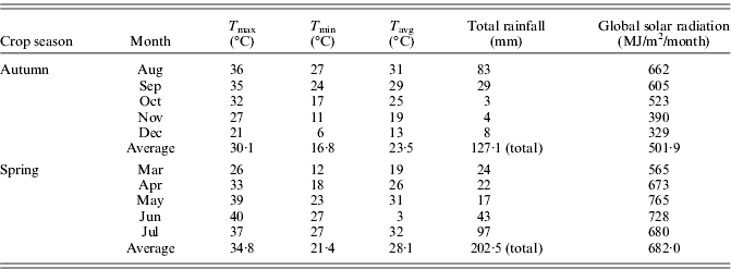
Irrigation experiments with maize (used for crop model calibration and validation in the present study) were conducted during 2007 for summer-sown maize (growing period: August–December) and during 2008 for spring-sown maize (growing period: March–July) at the experimental farm of the Institute of Soil and Environmental Sciences, University of Agriculture, Faisalabad, Pakistan (latitude 31°26′N, longitude 73°06′E, 184·4 m asl). The climate of the study area in Pakistan is subtropical semi-arid with >0·70 of the annual rainfall occurring from June through September. Mean monthly weather conditions of the period 1978–2008 for spring and autumn maize growing season are shown in Table 1.
Mean monthly weather conditions (baseline period 1978–2008) for spring and autumn maize growing season at Faisalabad, Pakistan
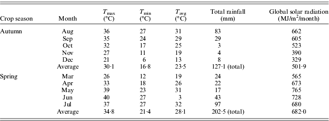
T max, maximum air temperature; T min, minimum air temperature; T avg, mean air temperature.
The soil at the experimental site is classified as a Typic Calciargid. Table 2 shows the basic soil properties of the experimental field, which were also used as input for the crop model. In both experimental years, the experimental field was irrigated uniformly before seeding to obtain field capacity (FC; 170 ml/l for Typic Calciargid soil) as a starting value and provide enough soil moisture for optimum germination. Seeding dates for summer-sown maize and spring-sown maize were 7 August 2007 and 20 March 2008, respectively. Flowering of summer-sown maize occurred on 14 October 2007, and spring-sown maize flowered on 28 May 2008. The harvest date for summer-sown maize was 8 December 2007 and for spring-sown maize was 10 July 2008.
Soil properties as input to the CERES maize model of the experimental field at Faisalabad, Pakistan

FC, field capacity; WP, wilting point.
Irrigation treatments consisted of providing a decreasing amount of water to the plants to study the transition from optimum water supply to sub-optimum moderate stress conditions. Water was applied with a hose to the experimental plots (flood irrigation). The amount of irrigation water required to maintain the soil water status at FC and the levels of the corresponding treatments was calculated based on the weekly measured soil water content readings using the following equation:
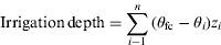
where θfc is the soil water content at FC (% by volume), θi is the soil water content (% by volume) before irrigation at soil depth i, z i is the depth of soil layer i (mm) and i is the number of soil layers (seven).
From this amount of water, which provides an optimum supply to the crop, a decreasing proportion was irrigated until the respective treatment (T) values were reached. The amount of water applied for summer-sown maize in 2007 were 339, 320, 210 and 150 mm, corresponding to T-0·85, T-0·80, T-0·55 and T-0·40 as partition of the amount of soil water at FC (FC=1), respectively. The irrigation treatments for spring-sown maize in 2008 consisted of the same treatments as in 2007 with an additional treatment of FC (T-1·00). The corresponding irrigation amounts in 2008 were 118 (T-1·00), 95 (T-0·85), 81 (T-0·80), 61 (T-0·55) and 49 mm (T-0·40). In addition to these schemes, 162 mm of irrigation water was applied nine times over the growing season at 18 mm per application. This was scheduled according to the ET-based estimation method of Allen et al. (Reference Allen, Pereira, Raes and Smith1998) and intended to avoid higher levels of water stress during the growing season. Irrigation scenarios for 2008 thus totals 280 (T-1·00), 257 (T-0·85), 243 (T-0·80), 223 (T-0·55) and 211 mm (T-0·40). These irrigation amounts did not give exactly the same proportional reductions as in the 2007 treatments; however, it still represented a stepwise increase in irrigation, starting from near-optimum and continuing through slightly sub-optimum levels. The soil water content at FC and the permanent wilting point were determined with a pressure membrane apparatus at 33 and 1500 kPa, respectively, at each depth (Cassel & Nielsen Reference Cassel, Nielsen and Klute1986). More experimental details are given in Iqbal et al. (Reference Iqbal, Bodner, Heng, Eitzinger and Hassan2010).
Use and calibration of the CERES-Maize model
The DSSAT crop models (Hoogenboom et al. Reference Hoogenboom, Jones, Wilkens, Batchelor, Bowen, Hunt, Pickering, Singh, Godwin, Bear, Boote, Ritchie and White1994), such as the CERES-maize model (Jones & Kiniry Reference Jones and Kiniry1986; Ritchie et al. Reference Ritchie, Singh, Godwin and Hunt1989), have been utilized extensively by agricultural scientists to study the impact of climate change and increasing levels of CO2 on yields of world crops (Rosenzweig et al. Reference Rosenzweig, Parry, Fischer and Frohberg1993).
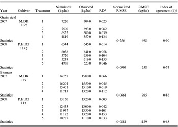
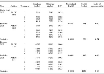
In the present field experiment for summer-sown maize in 2007 and spring-sown maize in 2008, the cultivars used were Monsanto DK119 and Pacific Hycorn ICI 11plus, respectively. As the maize cultivars were different in the two experimental years, the model was calibrated with the well-watered treatments and validated using the rest of the treatments (Table 3). An iterative procedure (Hunt et al. Reference Hunt, Pararajasingham, Jones, Hoogenboom, Imamura and Ogoshi1993) was used to select the most appropriate value for each phenological and developmental crop parameter (Table 4). After calibration and validation of the CERES-Maize model, the predefined reduced irrigation scenarios (Table 5) were simulated by the model for summer-sown maize in 2007 for the baseline period and the applied climate scenarios. Summer is the more productive season in this region for maize compared to spring because temperatures can reach a maximum of 35°C at the time of flowering during the spring season. Together with very high potential evapotranspiration, severe soil water deficits often are observed during these hot periods. Moreover, the growth rate per kernel of maize is reported to decrease with extremely high temperatures (Lorgeou Reference Lorgeou and Picard1990). Therefore, this simulation study was carried out for the preferred summer-sown maize in this region. The simulated CO2 effect, as used in this study by applied version 4.0.1 of the CERES-Maize model, can be seen as a maximum effect and does not consider new findings of potential environmental feedback, as discussed earlier. However, for C4 crops such as maize, only a moderate direct effect on the photosynthesis rate is considered in the crop model as compared to C3 crops such as cereals.
Observed and simulated grain yield and biomass of maize for both experimental years 2007 and 2008 (crop model validation results)
* RD, relative difference.
† Refers to Monsanto DK 119.
‡ Pacific Hycorn ICI 11 plus.
§ According to the d-statistics, the closer the index value is to one, the better the agreement between the two variables (i.e. simulated and observed yields in our case) that are being compared. Willmott et al. (Reference Willmott, Ackleson, Davis, Feddema, Klink, Legates, O'Connell and Rowe1985).
Crop coefficients used with the calibrated CERES-Maize model

P1: thermal time from seedling emergence to the end of the juvenile phase (expressed in degree days, °C, above a base temperature of 8°C) during which the plant is not responsive to changes in photoperiod.
P2: extent to which development (expressed as days) is delayed for each hour increase in photoperiod above the longest photoperiod at which development proceeds at a maximum rate (which is considered to be 12·5 h).
P5: thermal time from silking to physiological maturity (expressed in degree days above a base temperature 8°C).
G2: maximum possible number of kernels per plant.
G3: kernel filling rate during the linear grain filling stage and under optimum conditions (mg/day).
PHINT: phyllochron interval; the interval in thermal time (degree days) between successive leaf tip appearances.
Data source: Hoogenboom et al. (Reference Hoogenboom, Jones, Wilkens, Batchelor, Bowen, Hunt, Pickering, Singh, Godwin, Bear, Boote, Ritchie and White1994).
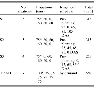
Reduced irrigation scenarios (S1, S2 and S3) used for crop simulation for summer-sown maize compared to the traditional local irrigation regime (TRAD). Irrigation was skipped at 45 DAS at vegetative stage for S1, at 105 DAS at grain filling stage for S2 and at crop establishment (25 DAS) stage and at grain filling stage (105 DAS) for S3. In all three scenarios 60 mm water was applied at each irrigation event and 75 mm water was applied at pre-planting
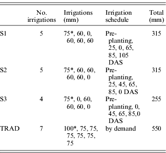
* Pre-planting irrigation; 0: No irrigation; S1, S2, S3: reduced irrigation regime scenarios; TRAD, traditional local irrigation regime; DAS, days after sowing.
Climate-change scenarios
Global circulation models (GCM) are useful tools for studying the impacts of climate change on agriculture (Betts & Falloon Reference Betts and Falloon2007). These models indicate a significant change in regional and seasonal climate patterns, which are predictive for the coming century (Gates et al. Reference Gates, Mitchell, Boer, Cubasch, Meleshko, Houghton, Callander and Varney1992). GCM scenarios, which simulate climate change as a function of time-dependent increases in CO2 concentrations, indicate that at current fossil fuel emission rates, a significant warming trend could be realized by the end of the next century (Houghton et al. Reference Houghton, Meiro Filho, Callander, Harris, Kattenberg and Maskell1996). Simulations with global climate models suggest that the projected increases in CO2 will modify the global climate by causing a widespread increase in the surface air temperature, by altering precipitation patterns and the global hydrologic cycle and by increasing the frequency of severe weather events, such as droughts and flooding (Houghton et al. Reference Houghton, Meiro Filho, Callander, Harris, Kattenberg and Maskell1996).
Climate-change projections for the present study were obtained from the general circulation model ECHAM5 (Roeckner et al. Reference Roeckner, Brokopf, Esch, Giorgetta, Hagemann, Kornblueh, Manzini, Schlese and Schulzweida2006). This is the latest version in a series of ECHAM Models. The spatial resolution of the GCM is 1·875×1·875 degrees, which leads to a grid spacing of c. 170 km east/west and c. 210 km north/south around the target region. Projections were achieved using the Climate and Environmental Retrieval and Archiving (CERA) data centre for A1B, A2 and B1 scenarios for three future 30-year periods, 2001–30, 2011–40 and 2036–65. Due to the steep gradient in the model orography between the Himalayas and the Indian Ocean, the climate-change signal was derived directly from the ECHAM5 grid-point in the area of Faisalabad, Pakistan. Downscaling methods using more GCM grid points were not applied (e.g. bilinear interpolation), as the neighbouring grid points represent the ocean or high mountainous regions.
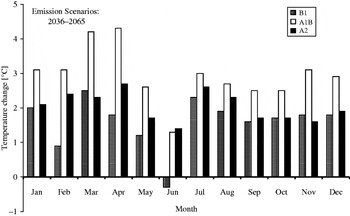
The climate-change signal was calculated on a monthly basis for temperature, precipitation and radiation. The climate-change signal is defined as the difference between the average values of the ECHAM5 control run (1978–2008) and the corresponding average values for the scenario periods. The time frame of the control period corresponded to the available field measurements. Figure 1 shows the mean monthly changes in temperatures for the three emission scenarios in the time period 2036–65, where the smallest temperature increase was seen during May and June, and higher temperature increases were observed for the A1B and A2 scenarios from January through April.
Monthly changes in temperatures for the three emission scenarios (A1B, A2 and B1) in the time period 2036–60.

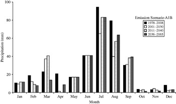
Precipitation at the selected ECHAM5 grid point, however, showed no significant annual variation, and monsoon precipitation, which contributes most of the annual precipitation, was extremely underestimated and was totally missing in May and June. The model precipitation for these 2 months was quite low (0 and 1·9 mm in the control period for May and June, respectively); therefore, the GCM-based relative changes in precipitation would have been very high and random. Thus, for these 2 months, no climatechange signal in precipitation was considered in the A1B scenario. Figure 2 shows the monthly precipitation changes applied for the A1B emission scenario for the different time periods. The changes in radiation were very low in the A1B scenarios, and the monthly variation was well below 1 MJ/m2/d. Because there was high uncertainty in the climate-change signal for precipitation and marginal changes in global radiation, only the temperature change from ECHAM5 is considered for local scenario construction for the B1 and A2 emission scenarios. Table 6 shows the applied annual changes in temperature, precipitation and radiation for the different climate scenarios, which were used for daily weather data calculations using a weather generator.
Applied monthly precipitation changes for the A1B emission scenario for the different time periods of the climate scenarios v. the control run period 1978–2008.

CO2 concentration, mean annual change in temperature, precipitation and daily global radiation for the different emission scenarios (SRES: B1, A1B, A2) and time frames of ECHAM 5 v. the control run period (1978–2008) for Faisalabad, Pakistan. The baseline CO2 concentration was set at 360 ppm

CO2, atmospheric carbon dioxide concentration; T, annual temperature change; P, change in annual precipitation; R, change in global radiation.
Weather generator LARS
The climate-change signals from GCM were derived on a monthly basis. Because the crop model CERES-Maize needs daily weather input data, the stochastic weather generator LARS-WG (Long Ashton Research Station Weather Generator; Semenov & Barrow Reference Semenov and Barrow1997) was used to convert the ECHAM5 climate-change signals into a local daily weather series. As a first step, the weather generator was calibrated using observational data, such as daily temperature, precipitation and global solar radiation from Faisalabad, Pakistan, for the period 1978–2008. For scenario construction, the monthly climate-change signals derived from ECHAM5 were added to the weather generator statistics in an additive way for temperature and radiation and in a multiplicative way for precipitation (radiation and precipitation signals were considered in the A1B scenario only). For every time section (control period and scenarios), a time series of 200 years of stable climate was produced and used for crop model simulations.
Crop simulations for autumn maize
The crop simulations with the crop model CERES-Maize were carried out in following steps:
(1) Executing the crop model with the baseline period (1978–2008; Table 1) to study the crop yield, water balance and CWP with CO2 concentration 360 ppm under three irrigation scenarios (Table 5). The three irrigation scenarios were defined as skipping irrigation (60 mm) at vegetative stage (S1), at grain filling stage (S2) and at crop establishment stage and grain filling stage (S3).
CWP was calculated by the following equations
(2) (3)where CWPET is crop water productivity based on evapotranspiration (kg/m3), CWPIR is crop water productivity based on irrigation water applied (kg/m3).
(2) Crop simulations were carried out for three climate-change scenarios (ECHAM 5 for emission scenarios A1B, A2 and B1) for the periods of 2001–30, 2011–40 and 2036–65 (Table 6) and for the three described irrigation scenarios. These simulations were carried out further with and without (constant level of 360 ppm for all climate scenarios assumed) consideration of atmospheric CO2 concentration changes on photosynthesis (hereafter referred to as the direct CO2 effect).
(3) To determine the optimum crop yield, water balance, CWP and water requirement for the above defined scenarios.


RESULTS
Simulated effects of reduced irrigation on maize growth and yield under the current conditions
Baseline simulations were carried out for weather characteristics of the reference period (1978–2008) for 200 generated weather years with an average atmospheric CO2 concentration of 360 ppm. Three irrigation scenarios with reduced irrigation rates were applied compared to local irrigation practices with a total irrigation of 550 mm for the autumn maize growing season (Table 5). Mean precipitation for the autumn maize growing season is up to 127 mm (Table 1), which is mainly at the beginning of the growing season (August and September). In the studied area, the maize cultivars used (summer-sown maize) usually complete their growing cycles within 120–125 days.
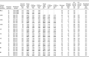
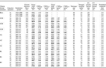
The baseline simulated crop growth duration (current conditions) of 119 days showed no change between irrigation scenarios (Table 7). Results showed that the highest grain yield (6760 kg/ha) was achieved in irrigation scenario S3 with less irrigation (60 mm) compared to the two other scenarios, S1 and S2 (with 315 mm of irrigation). Two irrigations were skipped in S3, one at crop establishment (25 days after sowing (DAS)) and the second at the grain-filling stage (105 DAS). The lowest grain yield (6102 kg/ha) was simulated in scenario S2, when irrigation was skipped at the grain-filling stage. The second-highest grain yield (6442 kg/ha) was simulated in scenario S1, where one irrigation was skipped at the vegetative stage. The simulation results showed clearly that the reduced irrigation in all three scenarios did not cause increased water stress because actual evapotranspiration was unchanged (Table 7). This shows that water was not a limiting factor, even in the reduced irrigation scenarios. Instead, increasing crop yields were simulated. Therefore, CWPET and CWPIR reached their highest values in scenario S3 with 2·65 and 2·01 kg/m3, respectively. Possible reasons why higher irrigation does not produce the highest grain yields in practice are that yield-limiting factors, such as less root development, unhealthy canopy structure and a lower harvest index or harvest ratio, increase. In the present study, lower N leaching rates in the reduced irrigation scenarios were found to be responsible for the simulated effect of increasing yields (Table 7), as no other yield-influencing simulated parameters, such as rooting depth or water stress, showed significant differences between the scenarios. Significant differences were found for deep drainage for all three irrigation scenarios, which supports the hypothesis for explaining simulated yield decreases for high irrigation rates. Generally, drainage is higher when irrigation plus rainfall exceed crop water requirements, which was the case in the simulation scenarios.
Simulated crop growth duration, yield, water balance parameters and crop water productivities for autumn maize under the applied reduced irrigation scenarios (S1, S2 and S3) for baseline and future climate change projections in Faisalabad, Pakistan
CWP, crop water productivity; ET, evapotranspiration; IR, irrigation.
Brackets with (*) and (†) sign indicate results for including direct CO2 effect and without direct CO2 effect of increased CO2 level, respectively. Bold characters highlight the highest values of the relevant parameter per emission scenario and period.
Overall, more drainage occurred in scenario S2 than in scenario S1 because in scenario S2, one irrigation was applied at the crop-development stage instead of at the grain-filling stage, when the crop has the highest water consumption. This leads to increased drainage during the irrigation event in the vegetative stage and in total. In scenario S3 (lowest total irrigation), the lowest amount of drainage occurred and higher grain yield (488 kg/ha), CWPET and CWPIR were achieved. The total rainfall in the months of August and September (during the vegetative stage) was 113 mm, which contributed to an optimum distribution and efficient use of water in this scenario and resulted in the highest grain yield and water productivities.
The simulated results for current conditions indicate that the highest grain yield and CWP can be achieved with less irrigation compared to current irrigation practices due to a lower N leaching rate.
Simulated effects of reduced irrigation on maize growth and yield in climate-change scenarios
The simulated growing period decreased in the climate scenarios compared to current conditions, which was sensitive to the climatic period as well as the emission scenarios. There are no differences in the simulated crop growth duration between the irrigation scenarios within emission scenarios in the same time period (Table 7). The most significant decrease in growing period was shown for 2036–65, with a decrease of 21 days in the A1B emission scenario in all irrigation scenarios. Not surprisingly, in the A1B emission scenario the lowest yield levels and crop water productivities were simulated in this period in all irrigation scenarios (Table 8). In the other two emission scenarios (A2 and B1), the decrease of yields and crop water productivities in the period 2036–65 compared to the periods 2001–30 and 2001–40 was much less, due to the lower temperature increases.
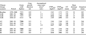
Simulated optimum maize grain yield and related crop growth duration, relative crop water stress of the whole growing period, water balance, CWP and irrigation amount with baseline and under climate change scenarios (autumn maize, Faisalabad, Pakistan)

* Relative crop water stress factor accumulated for various development stages; does not directly reflect stress impacts on crop yields due to different sensitivities in the various development stages.
CWP, crop water productivity; ET, evapotranspiration; IR, irrigation.
Bold characters represent the highest values of the relevant parameter per emission scenario and period.
The results show that in the climate scenarios, only increases in temperature caused significant decreases in crop growth duration, with a close relationship to yield decrease and crop water productivities. The differences within the applied irrigation scenarios are similar to current conditions (Table 7).
Results for emission scenario A1B
For emission scenario A1B in period 2001–30 (Table 7), the highest grain yield (6629 kg/ha) was simulated for irrigation scenario S3 with and without a direct CO2 effect (6878 kg/ha). This can be explained by the fact that the lowest N leaching rates were found in this irrigation scenario, as was previously shown for the current conditions. A CO2 level of 408 ppm produced 249 kg/ha higher yield than the unchanged CO2 level for the years 2001–30. For the period 2011–40, the highest grain yield was again reached in irrigation scenario S3, with 6907 kg/ha. With an increased CO2 level of 443 ppm, an additional yield of 303 kg/ha was achieved. Also the highest crop water productivities were achieved in this period.
The climate-change signal for the period 2036–65 (Table 6) shows a mean increase in temperature of 2·9°C and in solar radiation of 0·2 MJ/m2 per month compared to the control period 1978–2008 (baseline), which led to a growing period shortened by 21 days compared to the baseline and thus a lower yield.
The grain yield for this period was at 6396 kg/ha with a CO2 level of 536 ppm (5825 kg/ha without a change in CO2 level). Both CWPET and CWPIR were higher with increased CO2 fertilization compared to unchanged CO2 levels (Table 7), but decreased significantly compared to the periods 2001–30 and 2011–40 in spite of the highest CO2 level.
The highest CWPIR was achieved in irrigation scenario S3 for the period 2011–40 (2·70 kg/m3) with less irrigation, whereas evapotranspiration was also lower compared to unchanged CO2 levels. No significant differences were observed in cases of deep drainage with or without the direct CO2 effect; however, slightly higher drainage rates were observed for increased CO2 levels (Table 7).
Results for emission scenario A2
For scenario A2 over the period 2001–30 (Table 7), the highest grain yields were observed under irrigation scenario S3 (6660 kg/ha with unchanged CO2 levels and 6810 kg/ha with enhanced CO2 levels). With a CO2 level of 403 ppm, 150 kg/ha more yield was achieved. For the period 2011–40, the highest grain yield was again observed; 6872 kg/ha was achieved with current CO2 levels and the yield increased by 227 kg/ha for the 429 ppm CO2 level.
The climate change signal for the period 2036–65 showed an increase in temperature by 2·0°C compared to the baseline period, which led to a growing period shortened by 17 days compared to baseline, and thus, a lower yield level.
The grain yield for this period was 6797 kg/ha with a CO2 level of 507 ppm, and without a change in CO2 it was 6413 kg/ha. In contrast to the A1B scenario, the grain yield was decreasing only marginal compared to the 2001–30 and 2011–40 periods. With direct CO2 effect, CWPIR decreased slightly but increased for CWPET compared to the periods 2001–30 and 2011–40. Both CWPET and CWPIR were significantly higher with the direct CO2 effect compared to no change from the current CO2 level (Table 3). The highest CWPIR and CWPET were 2·67 and 2·15 kg/m3, respectively, achieved in irrigation scenario S3 in all periods. Again, the same trend was observed as in scenario A1B. There were no significant differences in simulated deep drainage with or without the direct CO2 effect, but slightly more drainage was observed under enhanced CO2 levels, as in the A1B emission scenario (Table 7).
Results for emission scenario B1
For scenario B1 in the period 2001–30 (Table 7), the highest grain yields were observed in irrigation scenario S3 (6659 kg/ha with the current CO2 level and 6815 kg/ha with an increased CO2 level). The increased CO2 level of 402 ppm resulted in 156 kg/ha higher yield. For the period 2011–40, the highest grain yield was again observed at 6807 kg/ha without a change in CO2. With an increased CO2 level of 427 ppm, the yield increased by 234 kg/ha.
The climate change signal for the period 2036–65 showed an increase in temperature by only 1·6°C and the growing season was shortened by 16 days in comparison with the baseline period, similar as in the A2 emission scenario.
The grain yield for this period was 6722 kg/ha at a higher CO2 level of 490 ppm and was at 6362 kg/ha with an unchanged CO2 level. There was also a small yield reduction simulated for the period 2036–65, as for the A2 emission scenario. With direct CO2 effect, CWPIR decreased slightly but CWPET increased compared to the periods 2001–30 and 2011–40. The highest CWP, lower ET and slightly higher deep drainage were observed with higher CO2 fertilization than with an unchanged CO2 level.
Irrigation scenario S3 again performed better in emission scenario B1, where the CWP reached 2·63 kg/m3 for CWPIR and 2·12 kg/m3 for CWPET.
Simulated optimum grain yield under current and future conditions
For the simulation of optimum grain yield, the automatic irrigation option of the CERES-Maize model was used, in which the model estimates the optimum irrigation schedule. As for the predefined irrigation scenarios (Table 7), the maize grain yields decreased under the future climate scenarios with the optimum irrigation schedule, however, higher yields and crop water productivities were achieved. For the current climate the optimum irrigation schedule increased grain yield to 7553 kg/ha with 285 mm of total irrigation and 373 mm of actual evapotranspiration (Table 8). The simulated results using the crop model to optimize the irrigation schedule show that under the current conditions, the addition of 30 mm of total irrigation water with an optimized distribution could further increase grain yield by 793 kg/ha and could also increase CWP compared to the best predefined irrigation scenario, S3. Using the model's suggested irrigation schedule for optimum yield, irrigation water demand would be reduced up to 236 mm for the period 2036–65, which had also the highest crop water productivities. This means that in the future climate scenarios, optimized irrigation will lead not only to higher yields, but also to lower irrigation rates compared to the best predefined irrigation scenario, S3, as shown in Table 8.
No significant differences in deep drainage were observed between emission scenarios and climate periods for optimum irrigation (Table 8), in contrast to the irrigation scenarios (Table 7). The simulated accumulated water stress factor is very low in all scenarios (Table 8), although there was an increasing trend with higher temperatures, and did not show a significant impact on the yield at this level. In the emission scenarios, actual evapotranspiration is reduced in the range of 15–50 mm for the periods of 2001–30, 2011–40 and 2036–65, which will cause yield reductions for future decades (Table 8). The decrease in yield levels using optimum irrigation scheduling for the periods 2001–30, 2011–40 and 2036–65 is caused mainly by shortened growing periods for the same cultivars.
DISCUSSION
With an average annual rainfall of 240 mm, Pakistan is one of the most arid countries in the world (World Bank 2006). Although it has the world's largest irrigation system (World Bank 2006), the agricultural sector has contributed only 0·20 of Pakistan's gross domestic product (GDP). The industrial sector of Pakistan accounted for 0·27 of the 2008 GDP, whereas 0·53 of the GDP came from the services sector. Pakistan's GDP was calculated to be c. $94.80 billion during 2003/04. This amount had gone up to $132.95 billion by fiscal year 2008/09. Pakistan still faces a substantial challenge in producing sufficient food to feed its growing population. Crop yields, in both per ha and per m3 water, are much lower than international benchmarks and much lower even than in neighbouring areas of India (World Bank 2006). An improvement in water management practices is therefore of the utmost importance to ensure food production with existing supplies of water.
Therefore, the present study applied the CERES-Maize model version 4.0.1 to different irrigation scenarios for summer-sown maize in order to identify optimum irrigation strategies under various climate-change scenarios.
The results reveal several interesting opportunities for better planning of autumn (summer-sown) maize irrigation in Pakistan. For example, it shows that for current conditions, as well as future climate scenarios, some of the usual irrigation events could be skipped in order to reach both higher yield levels and water savings. The predefined irrigation scenario S1, in which irrigation was skipped at the vegetative stage, should produce higher grain yield and CWP than irrigation scenario S2, in which irrigation was skipped at the grain-filling stage. Scenario S3, in which irrigation was skipped at crop establishment and the grain-filling stage, showed significantly higher yields with less water application (255 mm) than the other two scenarios, leading to the best CWP. The reason was that there was significantly less drainage and related N leaching in irrigation scenario S3 compared to the other two irrigation scenarios where there was excess water applied. When the model was executed for optimum grain yield (where the irrigation schedule was suggested by the crop model) for current conditions, a CWPET of 2·02 kg/m3 and CWPIR of 2·72 kg/m3 were reached, whereas the water requirement only amounted to 285 mm. This option also resulted in a significantly higher yield (increase by 793 kg/ha) under the current conditions than the best predefined irrigation scenario, S3.
Under the applied climate scenarios, the highest decrease in yield levels was shown for the period 2036–65 and for the A1B emission scenarios, which have the highest warming trends. In our simulation, the yield decrease was related to the significant shortening of the growing period. For example, the simulation showed that for 2036–65, the crop growth duration was shortened by up to 21 days (emission scenario A1B) compared to the baseline. Additionally, the growth rate per kernel of maize was reported to closely correlate with the mean daily temperature (Lorgeou Reference Lorgeou and Picard1990) and yield loss. Therefore, it is also a challenge for plant breeders to provide cultivars to the farmers that are adapted to be tolerant of temperature and water stress over long durations.
Furthermore, the results of the present study suggest that the yield of irrigated maize will be significantly affected by climate change in this semi-arid region, depending on the climate scenario. It is concluded that the combined effect of increases in temperature and CO2 concentration will shorten the growing cycle of maize under all emission scenarios, which is the main reason for the reduction in grain yield under warming climate. In future climate change emission scenarios, however, it is possible to further reduce irrigation demands due to reductions in actual crop evapotranspiration leading to increased CWP for the cultivars used. The study also reveals that current irrigation practices (for maize) can be significantly reduced in this location and under these soil conditions in order to reach higher yield levels, due to a reduction in N leaching. The present study shows that this effect can even outbalance the negative yield trend caused by the shortened growing period under the climate scenarios. In climate scenarios, an optimized irrigation schedule is therefore of growing importance in order to reduce absolute yield losses with a warming climate and to increase CWP for maize under similar agro-ecological conditions.
Uncertainties of the present study are especially related to applied climate scenarios and their predicted frequency of heat waves and crop model limitations (e.g. Eitzinger et al. Reference Eitzinger, Trnka, Hösch, Žalud and Dubrovský2003, Reference Eitzinger, Formayer, Thaler, Trnka, Zdenek and Alexandrov2008). For example, heat extremes may play an important role in this region in the future, especially for spring maize. Yan & Hunt (Reference Yan and Hunt1999) showed that with an increase in temperature to more than 41°C, maize cultivars exhibit negative responses that may lead to an accelerating frequency of crop failures not considered in the present study. In climate-change scenarios, higher potential ET is expected due to increasing temperatures (Monteith & Unsworth Reference Monteith and Unsworth1990); however, due to higher CO2 levels, a reduction in stomatal conductance (Lockwood Reference Lockwood1999) is expected. This could lead to higher leaf temperatures where critical thresholds could be exceeded earlier. In the present study, the shorter crop growth duration especially contributed to lower accumulated potential ET rates. Finally, these factors contribute to a reduction in actual ET and irrigation demands for the particular crop and cultivar. However, if adapted cultivars, such as more heat tolerant cultivars, replace current cultivars, irrigation demands could also increase in cases of reduced CWP of the specific cultivar.
From the present study it can be concluded that there is still an urgent need for more data for different treatments, locations and long-term field experiments to identify the best irrigation practices through validation of models that consider sensitive stages of each crop within a cropping cycle on the regional and national level. Further, the range of spatial and temporal variation of soil and climatic conditions should be considered to maximize the benefits of climate-change impact studies for advising potential adaptation options to the farmers on the local level. For this extrapolation, crop simulation models applied to climate scenarios are valuable tools.
We are greatly thankful to Mr Sahibzad Khan, Director, Regional Meteorological Centre, Lahore for providing long term weather data.