1. Introduction
Particle-laden turbulent channel flows exist widely in environmental phenomena such as turbidity currents (Salinas et al. Reference Salinas, Balachandar, Shringarpure, Fedele, Hoyal, Zuñiga and Cantero2021) and sandstorms (Liu, Shi & Zheng Reference Liu, Shi and Zheng2024), as well as in engineering applications like fuel–air mixing in the combustion chamber of scramjets (Ravindran et al. Reference Ravindran, Bricalli, Pudsey and Ogawa2019) and particle-based solar energy receivers (Tan & Chen Reference Tan and Chen2010; Pouransari & Mani Reference Pouransari and Mani2016). Especially, dispersed multiphase compressible turbulent flows are of great significance in engineering domains such as dust explosions and detonations (Capecelatro & Wagner Reference Capecelatro and Wagner2024). Dispersed multiphase turbulent flows are characterized by two interesting features, i.e. particle dispersion and clustering in the background flow and turbulence modulation by particles (Balachandar & Eaton Reference Balachandar and Eaton2010). Both features have been widely studied in incompressible flows during the last several decades. Readers are referred to review articles by Balachandar & Eaton (Reference Balachandar and Eaton2010) and Brand & Coletti (Reference Brand and Coletti2022) for further information about advancement in incompressible particle-laden turbulence.
Compared with its incompressible counterpart, there is relatively less research regarding particle-laden compressible turbulent channel flow (CTCF). The particle-laden CTCF can be studied from different aspects, including the particle behaviour, the turbulence modulation, the turbulence theory, etc. Li et al. (Reference Li, Cui, Yuan, Zhang, Zhou and Zhao2023) looked into the particle dynamics in CTCFs, and suggested that the compressibility effect tends to amplify particle velocities. Wang, Zhou & Zheng (Reference Wang, Zhou and Zheng2024) demonstrated that the wall accumulation of inertial particles caused by turbophoresis in CTCFs is reduced when the Mach number is very high. As for the turbulence modulation, only very preliminary results are reported recently (Ruan & Xiao Reference Ruan, Xiao, Zheng and Balachandar2024a ) based on a Eulerian–Lagrangian point-particle (PP) simulation. In other words, investigation on turbulence modulation caused by inertial particles in CTCFs is still in its infancy. There are, in addition, very few turbulence theories regarding particle-laden CTCFs reported in the literature.
Unlike particle-laden CTCFs, single-phase CTCFs have experienced vigorous development with various theoretical models. One of the most famous turbulence theories in CTCFs is the strong Reynolds analogy (Reynolds Reference Reynolds1874, reprinted in Reynolds Reference Reynolds1961), which describes the mean velocity–temperature relation and is one of the most important theoretical conceptions in compressible wall-bounded turbulence. Busemann (Reference Busemann1931) and Crocco (Reference Crocco1932) independently established the mean velocity–temperature relation in a compressible zero-pressure-gradient laminar boundary layer with an adiabatic wall of unity Prandtl number, which is now known as the Crocco–Busemann relation. The development of the Reynolds analogy can be categorized into two brunches, i.e. the analogical method (Young Reference Young1951) and the analytical method (van Driest Reference van Driest1955). The former develops the mean velocity–temperature relation of unity Prandtl number by the similarity between averaged velocity and temperature equations. The latter extends the Crocco–Busemann relation to zero-pressure-gradient turbulent boundary layer with non-constant Prandtl number and adiabatic wall by analytically solving a modelled ordinary differential equation (van Driest Reference van Driest1955). Walz’s equation depicts a mean velocity–temperature profile with Prandtl number deviating from unity by introducing recovery enthalpy and a corresponding recovery factor (Walz Reference Walz1969). Zhang et al. (Reference Zhang, Bi, Hussain and She2014) further extend Walz’s equation to wall-bounded turbulence under different wall conditions and pressure gradient by defining generalized recovery enthalpy. The history and development of the mean velocity–temperature relation in wall-bounded turbulence are summarized by Fernholz & Finley (Reference Fernholz and Finley1980). Another important aspect of the Reynolds analogy is about the fluctuating velocity–temperature relation (Morkovin Reference Morkovin1962; Rubesin Reference Rubesin1990; Huang, Coleman & Bradshaw Reference Huang, Coleman and Bradshaw1995; Zhang et al. Reference Zhang, Bi, Hussain and She2014). However, the focus of this paper is placed on the mean temperature–velocity relation. The extension of the Reynolds analogy to particle-laden CTCFs is helpful in understanding and predicting the turbulence modulation caused by inertial particles.
The turbulence modulation caused by inertial particles is mostly referred to the attenuation or amplification of velocities in the reported literatures in either CTCF or its incompressible counterpart. While velocity is the most representative and important physics variable to characterize turbulence, temperature is another significant dimension in describing compressible turbulence, which can certainly not be ignored. For a calorically perfect gas with constant specific heat capacity regardless of temperature change, such as air, the velocity and temperature represent two essential forms of energy, respectively, i.e., the kinetic energy and internal energy. The transform between these two types of energy is known to be at a central place in aerodynamics studies (Mittal & Girimaji Reference Mittal and Girimaji2019; Fan, Li & Pirozzoli Reference Fan, Li and Pirozzoli2022), where the compressible wall-bounded turbulence is frequently involved. In particular, the temperature evolution in CTCFs is influenced by the density stratification and boundary conditions of temperature at the wall. In other words, temperature is a very important aspect in describing CTCFs. Therefore, one cannot simply study the modulation of kinetic energy (or the velocities) without taking insight into the modulation of internal energy (or the temperature) if the aim is to investigate the turbulence modulation caused by inertial particles in CTCFs.
The objective of the research reported in this paper is threefold. First, we plan to extend Reynolds analogy to particle-laden CTCFs. Second, we want to study the velocity and temperature modulations of turbulence caused by inertial particles. Third, we intend to unveil the physics mechanism of turbulence modulation through the energy transfer analysis. In order to realise these goals, numerical simulations of CTCFs are carried out using the two-way coupling PP method. The particles are assumed to be identical small spheres. Due to the small particle size, the rotation and volume of particles can be neglected. The particles are presumed to be adiabatic, i.e. there is no heat transfer between particles and the carrier fluids. The gravity is left aside for now to avoid particle sediment (Peng, Wang & Chen Reference Peng, Wang and Chen2024).
The remaining paper is structured as follows. Introduced in § 2 are the governing equations, numerical methods and numerical settings for two-way coupling PP direct numerical simulation (DNS) (abbreviated as PP-DNS hereafter) of CTCFs. In particular, a validation test of single-phase CTCFs is provided in § 2.4. The Reynolds analogy is established and validated for both single-phase and particle-laden CTCFs in § 3. The turbulence modulation caused by heavy particles is presented in § 4. Meanwhile, the quantitative description and theoretical prediction for the modulation of mean temperature are also offered in § 4. The transform between the kinetic energy of the dispersed phase/carrier phase and the internal energy of the carrier phase is analysed in § 5, which sheds light on the underlying mechanism of the velocity and temperature modulation caused by particles. Finally, concluding remarks and discussions are given in § 6.
2. Simulation details
In the present study, two-way coupling PP-DNS is conducted to investigate turbulence modulation caused by heavy particles in fully developed CTCF. First of all, the PP hypothesis requires that the particle diameter is smaller than the smallest length scale in the turbulent channel flow. Furthermore, the two-way coupled particle–turbulence interaction is valid only when the particle mass fraction is larger than
 $10^{-3}$
and the particle volume fraction is smaller than
 $10^{-3}$
, to neglect the effect of particle collisions. In addition, the particle motion equation is a simplified version for heavy particles, i.e. the particle-to-fluid density ratio is larger than
 ${O}(10^3)$
.
The governing equations for the carrier and dispersed phases are given in §§ 2.1 and 2.2, respectively. The detailed parameters of CTCF and particles are described in § 2.3, where the numerical methods employed to solve the governing equations are also introduced. The numerical simulation of single phase CTCF is validated in comparison with the numerical data from Coleman, Kim & Moser (Reference Coleman, Kim and Moser1995) in § 2.4 .
2.1. Governing equations of carrier phase
The carrier phase of particle-laden CTCF is described by the compressible Navier–Stokes equations, including the equation of continuity, equation of momentum and equation of total energy, which read
 \begin{align} \frac{\partial \rho }{\partial t} + \frac{\partial \rho u_{\!j}}{\partial x_{\!j}} &= 0, \end{align}
 \begin{align} \frac{\partial \rho u_i}{\partial t} + \frac{\partial \rho u_i u_{\!j}}{\partial x_{\!j}} = -\frac{\partial p}{\partial x_i} &+ \frac{\partial \sigma _{\textit{ij}}}{\partial x_{\!j}} + \rho f_i - \rho \varphi _i, \end{align}
 \begin{align} \frac{\partial \!E}{\partial t} + \frac{\partial (E+p) u_{\!j}}{\partial x_{\!j}} = - \frac{\partial q_{\!j}}{\partial x_{\!j}} &+ \frac{\partial \sigma _{\textit{ij}}u_i}{\partial x_{\!j}} +\rho f_i u_i - \rho \varphi _e, \end{align}
with
 $\rho$
,
 $u_i$
and
 $p$
being the density, velocity and pressure of the fluid, respectively. The viscous stress tensor is written as
 \begin{equation} \sigma _{\textit{ij}} = 2 \mu ({\mathcal{S}}_{\textit{ij}}-{\mathcal{S}}_{ll}\delta _{\textit{ij}}/3), \end{equation}
with
 $\mu$
being the dynamic viscosity of the fluid and
 ${\mathcal{S}}_{\textit{ij}} = ({\partial u_i}/{\partial x_{\!j}} \!+\! {\partial u_{\!j}}/{\partial x_i})/2$
the strain rate tensor.
The equation of state for an ideal gas is employed to close the pressure, i.e.
 $p=\rho r_0 T$
with
 $r_0$
being the specific gas constant and
 $T$
the temperature. Here
 $E = e + \rho u_i u_i/2$
is the total energy of the fluid, where
 $e$
represents the internal energy. By definition, the internal energy can be expressed by the fluid temperature as
 $e = \rho C_V T$
, with
 $C_V$
being the specific heat at constant volume. The heat flux
 $q_{\!j}$
is expressed as
 \begin{equation} q_{\!j} = -\kappa \frac{\partial T}{\partial x_{\!j}}, \end{equation}
with
 $\kappa$
being the conductivity of the fluid. The conductivity and viscosity are connected by the Prandtl number, defined as
 ${\textit{Pr}} \equiv C_{\!p} \mu /\kappa$
, with
 $C_{\!p}$
being the specific heat at constant pressure. In compressible flows, the viscosity is dependent on the temperature of the fluid. The viscosity can be obtained based on Sutherland’s law in the form
 \begin{equation} \mu = \mu _0\left (\frac{T}{T_0}\right )^{1.5} \frac{T_0+T_s}{T+T_s}, \end{equation}
where
 $\mu _0$
is the reference viscosity at reference temperature
 $T_0$
, and
 $T_s = 110.4\, {\textrm{K}}$
is the Sutherland temperature. The channel flow is driven by an external uniform body force
 $f_i$
(Coleman et al. Reference Coleman, Kim and Moser1995) to maintain a constant bulk velocity, which is obtained by a relaxation algorithm proposed by Lenormand, Sagaut & Ta Phuoc (Reference Lenormand, Sagaut and Ta Phuoc2000). Here
 $\varphi _i$
and
 $\varphi _e$
are the particle feedback terms on the fluid whose expressions are to be given in § 2.2.
2.2. Governing equations of dispersed phase
The inertial particles are assumed to be identical solid spheres of density
 $\rho _{\!p}$
and diameter
 $d$
. The particles under consideration are adiabatic, and therefore there is no heat transfer between dispersed and carrier phases. The motion of inertial particles follows the Tsai–Maxe–Riley equation (Tsai Reference Tsai1956; Maxey & Riley Reference Maxey and Riley1983, reprinted in Tsai (Reference Tsai2022)). The Tsai–Maxey–Riley equation is dominated by Stokes drag (Stokes Reference Stokes1850) when the particle-to-fluid density ratio is over
 ${O}(10^3)$
(Armenio & Fiorotto Reference Armenio and Fiorotto2001). What is more, the shear-induced lift (Saffman Reference Saffman1965, Reference Saffman1968) proves to be significant when particle diameter in wall unit exceeds
 $0.4$
(Ruan & Xiao Reference Ruan and Xiao2024b
). As a result, the equations of particle motion read
 \begin{align} \frac{{\textrm{d}} \boldsymbol{x}_{\!p}}{{\textrm{d}} t} &= \boldsymbol{u}_{\!p}, \end{align}
 \begin{align} \boldsymbol{a}_{\!p} \equiv \frac{{\textrm{d}} \boldsymbol{u}_{\!p}}{{\textrm{d}} t} = \frac{C_{\!D} {\textit{Re}}_{\!p}}{24\tau _{\!p}} \left [ \boldsymbol{u} ( \boldsymbol{x}_{\!p} ) - \boldsymbol{u}_{\!p} \right ] & + \frac{6.46}{\tau _{\!p}} \frac{d}{12\pi } \left ( \frac{\rho }{\mu |\boldsymbol{\omega }|} \right )^{1/2} \boldsymbol{\omega } \times \left [ \boldsymbol{u} ( \boldsymbol{x}_{\!p} ) - \boldsymbol{u}_{\!p} \right ]\!, \end{align}
with
 $\boldsymbol{x}_{\!p}$
being the particle position in the flow field,
 $\boldsymbol{u}_{\!p}$
the particle velocity,
 $\boldsymbol{a}_{\!p}$
the particle acceleration and
 $\boldsymbol{u} ( \boldsymbol{x}_{\!p} )$
the fluid velocity seen by the particle. The particle relaxation time is calculated as
 $\tau _{\!p} \equiv \rho _{\!p} d^2 /(18 \mu )$
. The Stokes number
 $St$
, a dimensionless parameter characterizing the inertia of particles, is defined as the ratio of
 $\tau _{\!p}$
to the fluid characteristic time
 $\tau _f$
(e.g. the Kolmogorov time scale of background turbulence). The second term on the right-hand side of (2.8) is the shear-induced lift (Saffman Reference Saffman1965, Reference Saffman1968), where
 $\boldsymbol{\omega }$
is local vorticity of the fluid phase.
The first term on the right-hand side of (2.8) is the Stokes drag, with
 $C_{\!D}$
being the correction coefficient of the drag and
 ${\textit{Re}}_{\!p} \equiv \rho |\boldsymbol{u} ( \boldsymbol{x}_{\!p} ) - \boldsymbol{u}_{\!p}| d /\mu$
the particle Reynolds number. Schiller & Naumann (Reference Schiller and Naumann1933) suggest the finite Reynolds number correction for inertial particles, but ignore the compressibility effect on the Stokes drag. Loth (Reference Loth2008) demonstrates that the compressibility effect and rarefaction effect on particle motion cannot be neglected when the particle Mach number
 ${\textit{Ma}}_{\!p} \equiv |\boldsymbol{u} ( \boldsymbol{x}_{\!p} ) - \boldsymbol{u}_{\!p}|/c$
and particle Knudson number
 ${\textit{Kn}}_{\!p} \equiv \sqrt {\pi \gamma /2} {\textit{Ma}}_{\!p}/{\textit{Re}}_{\!p}$
are important, where
 $c$
is the sound speed at the particle position, and
 $\gamma \equiv C_{\!p}/C_V$
is the ratio of specific heats. The compressibility effect on particles can be neglected when particle Mach number is smaller than 0.4. However, the values of
 ${\textit{Ma}}_{\!p}$
in some cases of present study are much larger than this limit. Therefore, the compressibility correction must be included in
 $C_{\!D}$
. Likewise, although the fluid Knudson number is very small in CTCF, the particle Knudson number can be of order
 ${O}(1)$
in present configuration, and hence, the rarefaction correction cannot be disregarded. Consequently, the compressibility and rarefaction corrected drag coefficient
 $C_{\!D}$
suggested by Loth, Daspit & Jeong (Reference Loth, Daspit and Jeong2021), which is valid for
 ${\textit{Re}}_{\!p}\leqslant 45$
(rarefaction-dominated regime), is employed in present simulations in the form
 \begin{equation} C_{\!D} = \frac{C_{\!D,Kn,{\textit{Re}}}}{1+{\textit{Ma}}_{\!p}^4} + \frac{{\textit{Ma}}_{\!p}^4 C_{\!D,\textit{fm},{\textit{Re}}}}{1+{\textit{Ma}}_{\!p}^4}, \end{equation}
where
 $C_{\!D,Kn,{\textit{Re}}}$
and
 $C_{\!D,fm,{\textit{Re}}}$
are, respectively, the low-Mach-number-limit and high-Mach-number-limit of drag correction in the rarefaction-dominated regime. At low Mach number, the Schiller–Naumann correction (Schiller & Naumann Reference Schiller and Naumann1933) is modified with the Knudson number effect as
 \begin{equation} C_{\!D,Kn,{\textit{Re}}} = \frac{24}{{\textit{Re}}_{\!p}} \left (1+0.15 {\textit{Re}}_{\!p} ^{0.687}\right ) f_{Kn}, \end{equation}
where
 $f_{Kn}$
is developed by Clift & Gauvin (Reference Clift and Gauvin1971) and takes the form
 \begin{equation} f_{Kn} = \frac{1}{1+{\textit{Kn}}_{\!p} \left [ 2.514 + 0.8 \exp \left (-0.55\!/\!{\textit{Kn}}_{\!p}\right ) \right ]}. \end{equation}
At high Mach number, the free-molecular limit correction for finite Reynolds number takes the form
 \begin{align} C_{\!D,fm,{\textit{Re}}} & = \frac{C_{\!D,\textit{fm}}}{1+[(C_{\!D,\textit{fm}}/J_M)-1]\sqrt {{\textit{Re}}_{\!p}/45}}, \end{align}
 \begin{align} J_M & = \left \{ \begin{array}{ll} \displaystyle 2.26 - \frac{0.1}{{\textit{Ma}}_{\!p}} + \frac{0.14}{{\textit{Ma}}_{\!p}^3} & \mbox{for } {\textit{Ma}}_{\!p} \leqslant 1, \\ \displaystyle 1.6 +\frac{0.25}{{\textit{Ma}}_{\!p}} + \frac{0.11}{{\textit{Ma}}_{\!p}^2} + \frac{0.44}{{\textit{Ma}}_{\!p}^3} & \mbox{for } {\textit{Ma}}_{\!p} \gt 1,\\ \end{array} \right . \end{align}
with
 $C_{\!D,\textit{fm}}$
being the free-molecular limit at a molecular speed ratio
 $s\equiv {\textit{Ma}}_{\!p} \sqrt {\gamma /2}\gt 1$
(Stadler & Zurick Reference Stadler and Zurick1951), which is defined as
 \begin{equation} C_{\!D,\textit{fm}} = \frac{(1+2s^2)\exp (-s^2)}{s^3\sqrt {\pi }} + \frac{(4s^4+4s^2-1)\textrm {erf}(s)}{2s^4} + \frac{2}{3s}\sqrt {\pi }. \end{equation}
The two-way coupling feedback effect of particles on fluid momentum is modelled as a body force
 $\varphi _i$
. The particle source-in-cell strategy (Crowe, Sharma & Stock Reference Crowe, Sharma and Stock1988) is used to distribute feedback force to the nearest grid point to a particle. The kinetic energy exchange between particles and fluids is described by
 $\varphi _e$
. The expression of feedback terms in a grid cell domain
 $\varOmega$
can be written as
 \begin{align} \varphi _i &= \frac{\pi d^3}{6} \frac{\rho _{\!p}}{\rho } \sum \limits _{n \mbox{ in } \varOmega } {H\big(\boldsymbol{x}-\boldsymbol{x}_{\!p}^n\big) a_{p,i}}, \end{align}
 \begin{align} \varphi _e &= \frac{\pi d^3}{6} \frac{\rho _{\!p}}{\rho } \sum \limits _{n \mbox{ in } \varOmega } {H\big(\boldsymbol{x}-\boldsymbol{x}_{\!p}^n\big) a_{p,i} u_i}, \end{align}
with the weight function
 \begin{equation} H(\boldsymbol{x}-\boldsymbol{x}_{\!p}) = \left \{ \begin{array}{ll} 1/\Delta\!V & \mbox{if the particle is in present grid cell}, \\ 0 & \mbox{otherwise,} \end{array} \right . \end{equation}
where
 $\Delta\!V$
represents the volume of the computational grid cell.
2.3. Numerical set-ups
First of all, CTCF is simulated to a fully developed state though the DNS method. The fluid is set as air with a Prandtl number of approximately
 $0.7$
. The channel size is
 $L_x \times L_y \times L_z = 4\pi \delta \times 2\delta \times 4\pi \delta /3$
with
 $\delta$
denoting the half-width of the channel, and
 $x$
,
 $y$
and
 $z$
representing the streamwise, wall-normal and spanwise directions of the channel, respectively. Non-slip boundary conditions are applied at the walls. The periodic boundary conditions are imposed in the streamwise and spanwise directions. Specifically, both bottom and top walls are set as isothermal cold walls in the present simulations as done by Coleman et al. (Reference Coleman, Kim and Moser1995). A perturbed laminar parabolic Poiseuille velocity profile is imposed as the initial velocity condition. The governing equations for the carrier phase are solved by the open-source code Opencfd-SC based on a finite difference method (Zhang et al. Reference Zhang, Guo, Dang and Li2024). The numerical flux is split by using Steger–Warming method (Steger & Warming Reference Steger and Warming1981). A hybrid scheme of seventh-order linear scheme and high-order weighted essentially non-oscillatory scheme based on a modified Jameson discontinuity sensor (Ji et al. Reference Ji, Li, Tong and Yu2023) is used to discretize the convection term. The viscous term is discretized by an eighth-order central difference scheme. The governing equations are advanced through a third-order total variation diminishing Runge–Kutta multistage time integration (Shu & Osher Reference Shu and Osher1988).
The Reynolds number
 ${\textit{Re}}$
is defined based on the free stream velocity, viscosity, density and half-width of the channel. The Mach number
 ${\textit{Ma}}$
is defined using free stream velocity and sound speed at the wall. Three cases of different Reynolds and Mach numbers are simulated in present study. The friction Reynolds number is defined as
 ${\textit{Re}}_{\tau } = \rho _w u_{\tau } \delta / \mu _w$
with
 $\rho _w = \overline {\rho }_w$
being the mean fluid density at the wall,
 $\mu _w = \overline {\mu }_w$
the mean fluid viscosity at the wall,
 $u_{\tau } \equiv \sqrt {\tau _w/\rho _w}$
the friction velocity and
 $\tau _w$
the total shear stress at the wall. The distance to the wall in wall units (denoted by
 $y^+$
) is defined as that normalized by wall viscous scale
 $\delta _{\nu } = \mu _w / (\rho _w u_{\tau })$
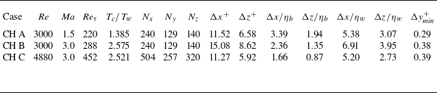
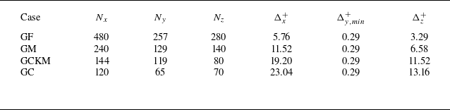
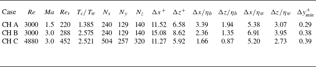
. Summarized in table 1 are the input dimensionless parameters for simulations of channel flows in this study. The computational domain is uniformly discretized in the streamwise and spanwise directions, whereas the wall-normal direction is resolved by a stretched mesh refined by a hyperbolic tangent function. The grid numbers and grid sizes (in wall units) in various directions are also listed in table 1. The wall-normal size of the nearest grid to the wall, denoted by
 $\Delta y_\textit{min}^+$
, is smaller than 1, which allows one to resolve the viscous sublayer of the flows. To further strengthen the validity of present numerical simulations, ratios of gird sizes in the streamwise and spanwise directions to the bulk Kolmogorov scale (
 $\eta _b$
, defined based on the bulk dissipation, viscosity and density) and the Kolmogorov scale (
 $\eta _w$
, defined based on the local dissipation, viscosity and density) at the wall are calculated for cases CH A, CH B and CH C, which are also listed in table 1. While the grid spacings in the streamwise and spanwise directions in wall units for CH A are similar to those employed by Kim, Moin & Moser (Reference Kim, Moin and Moser1987), which are
 $\Delta x^+\approx 12$
and
 $\Delta z^+\approx 7$
, respectively, the corresponding grid sizes for CH B are relatively large in comparison with the former. However, the relative grid sizes compared with the bulk Kolmogorov scale in wall parallel directions for both CH A and CH B are smaller than those calculated by Kim et al. (Reference Kim, Moin and Moser1987), which are
 $\Delta x/\eta _b\approx 6$
and
 $\Delta z/\eta _b\approx 3.5$
, respectively. These seemingly contradictory results stem from the fact that fluid viscosity experiences variation across the channel width in compressible channel flow, i.e. successively increasing from the wall to the channel centre, while it remains unchanged in the incompressible case. If one measures the grid spacings in Kolmogorov scale at the wall, it turns out that the streamwise grid size for CH B is slightly larger than that from Bernardini, Pirozzoli & Orlandi (Reference Bernardini, Pirozzoli and Orlandi2014), while the spanwise grid size is similar to that used by Bernardini et al. (Reference Bernardini, Pirozzoli and Orlandi2014), which are
 $\Delta x/\eta _b\leqslant 6.5$
and
 $\Delta z/\eta _b\leqslant 4.5$
, respectively. In general, present gird resolutions are sufficient to resolve the turbulent channel flows under consideration.
Input parameters and grid sizes for single-phase CTCFs.
Once the CTCFs reach a fully developed state, inertial particles are uniformly seeded into the flow field. The initial velocities of particles take the values of fluid velocities at the same positions. In the simulations, particles that collide with the wall are subjected to a reflection by preserving their velocity components in the streamwise and spanwise directions, while reversing the wall-normal velocity component. In instances where particles depart from the computational domain in either streamwise or spanwise directions, they are reintegrated into the channel through periodic boundary conditions with their velocities remaining unchanged. The governing equations of particle motion are advanced by using the second-order Adams–Bashforth scheme. The fluid information is interpolated onto particles by the third-order Lagrange interpolation scheme. The numerical results are obtained once the particle distribution within the channel has attained a statistically steady state.
As aforementioned, particle inertia is evaluated by the ratio of particle relaxation time to Kolmogorov time scale at the central plane, i.e.
 $St = \tau _{\!p}/\tau _{k,cp}$
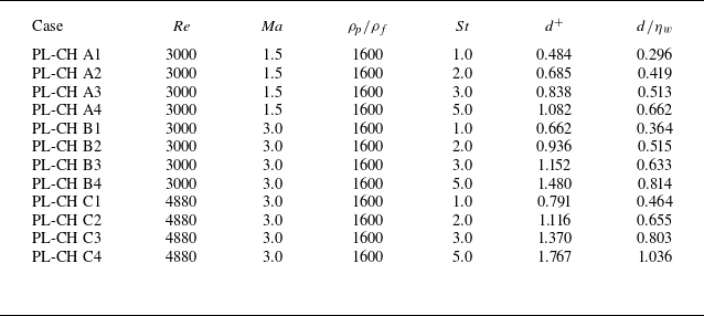
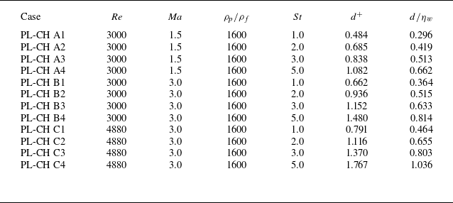
. Monodispersed particle-laden CTCFs are numerically simulated in this research work. The inertias of solid particles are different from one case to another. The particle-to-air density ratio is fixed to 1600, which is a characteristic value of mass density ratio between sand and air. The particle diameters corresponding to different Stokes number are displayed in table 2. The particle diameters of concern in this study are all smaller than the smallest turbulence scale (i.e. the Kolmogorov length scale at the wall
 $\eta _w$
), which validates the PP hypothesis. Besides, it can be observed that some particle diameters in wall unit
 $d^+$
are larger than
 $0.438$
, the critical value over which shear-induced lift needs to be included (Ruan & Xiao Reference Ruan and Xiao2024b
). Last but not least, it has been revealed by experimental research that the mass loading rate of particles has a massive influence on turbulence modulation in incompressible turbulent channel flow (Kulick, Fessler & Eation Reference Kulick, Fessler and Eation1994). Therefore, the particle numbers are adjusted in different cases such that the corresponding particle mass fractions share the same value. Specifically, the particle mass fraction is set to 0.1 in the present research work.
Input parameters for particle-laden CTCFs.
2.4. Validation of single-phase channel flow
The simulation cases CH A and CH C in this study have the same physical parameters as cases A and B, respectively, reported by Coleman et al. (Reference Coleman, Kim and Moser1995). Therefore, the present code is validated by comparing the numerical results of cases CH A and CH C with the DNS data presented in the literature. In what follows, both ensemble (Reynolds) average and density-weighted (Favre) average are introduced in presenting statistical results from current DNS. Taking the streamwise velocity
 $u$
as an example,
 $\overline {u}$
represents the Reynolds-averaged streamwise velocity of fluid and
 $u^{\prime} \equiv u - \overline {u}$
is the corresponding fluctuation. Meanwhile,
 $\widetilde {u} \equiv \overline {\rho u }/\overline {\rho }$
denotes the Favre-averaged streamwise velocity with
 $u^{\prime \prime} \equiv u - \widetilde {u}$
being the corresponding fluctuation.
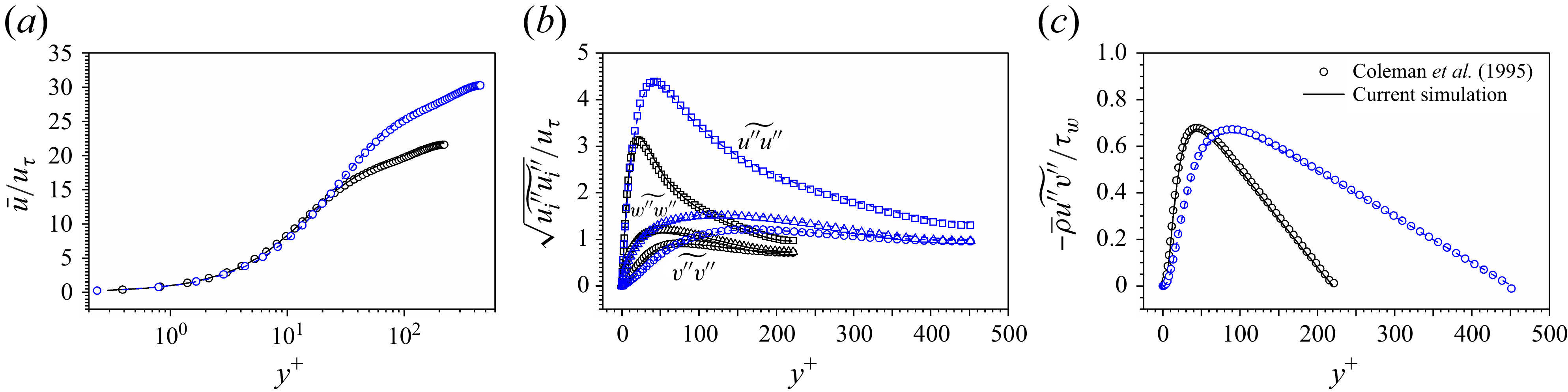
Profiles of (a) mean streamwise velocity of fluid phase, (b) r.m.s density-weighted fluctuating velocities and (c) Reynolds stress computed in present simulations of case CH A (black solid lines) and case CH C (blue dashed lines). The numerical data from Coleman et al. (Reference Coleman, Kim and Moser1995) are also included (symbols) for comparison.
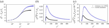
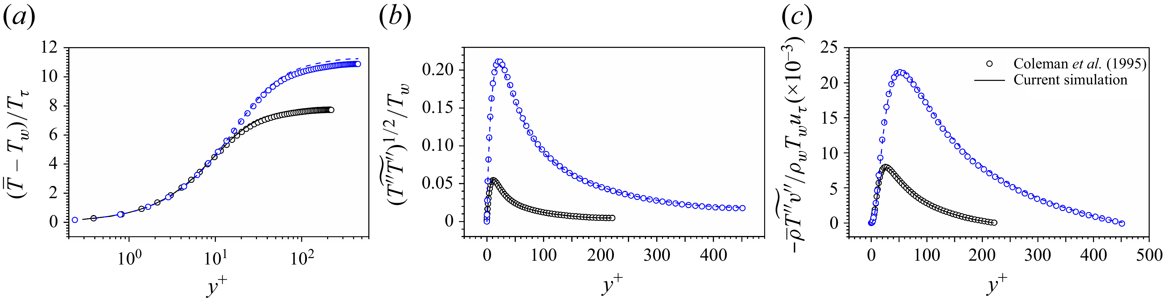
Profiles of (a) mean temperature, (b) r.m.s density-weighted fluctuating temperature and (c) Reynolds heat flux computed in present simulations of case CH A (black solid lines) and case CH C (blue dashed lines). The numerical data from Coleman et al. (Reference Coleman, Kim and Moser1995) are also provided (symbols) for comparison.
The profiles of Reynolds-averaged streamwise velocity normalized by wall friction velocity
 $\overline {u}^+ \equiv \overline {u}/u_{\tau }$
are displayed in figure 1(a). The numerical results show that current DNS data agree very well with those from Coleman et al. (Reference Coleman, Kim and Moser1995). Depicted in figure 1(b) are the Favre-averaged root-mean-square (r.m.s) velocity fluctuations normalized by
 $u_{\tau }$
. The numerical results obtained by current DNS are represented by lines. The profiles of velocity fluctuations from Coleman et al. (Reference Coleman, Kim and Moser1995) are represented by squares, circles and triangles, respectively. Again, current DNS data are in very good accordance with those given by Coleman et al. (Reference Coleman, Kim and Moser1995). Figure 1(c) shows the Reynolds stress
 $-\overline {\rho }\widetilde {\ u^{\prime \prime}v^{\prime \prime}}$
normalized by wall shear stress
 $\tau _w$
. It is clear that current DNS can successfully reproduce the results from the literature.
In CTCFs, the profiles of temperature and temperature fluctuations are also of great importance for the validation of numerical simulations. Depicted in figure 2(a) are profiles of mean temperature
 $\overline {T}^+=(\overline {T}-T_w)/T_{\tau }$
, with
 $T_w$
being the constant wall temperature,
 $T_{\tau } = -B_q T_w$
the friction temperature,
 $B_q = q_w/(\rho _w C_{\!p} u_{\tau } T_w)$
the dimensionless heat flux and
 $q_w$
the wall heat flux. The profiles of r.m.s temperature fluctuations normalized by wall temperature and the Reynolds heat flux
 $-\overline {\rho }\widetilde {T^{\prime \prime}v^{\prime \prime}}$
normalized by
 $\rho _w T_w u_{\tau }$
are shown in figures 2(b) and 2(c). The discrepancy in centreline temperature between present numerical simulations and that from Coleman et al. (Reference Coleman, Kim and Moser1995) is mainly attributed to different numerical methods. Despite such differences, the reliability of the present code can still be verified by comparing current results with those reported by Coleman et al. (Reference Coleman, Kim and Moser1995).
3. Reynolds analogy
In this section, the Reynolds analogy is first extended to multiphase CTCFs by solving an ordinary differential equation. Then, the theory is validated in both single-phase and multiphase CTCFs.
3.1. Establishment of Reynolds analogy
In order to obtain the relation between streamwise velocity and temperature, we work with the equation of momentum in the streamwise direction and the equation of enthalpy derived from (2.2) and (2.3),
 \begin{equation} \frac{\partial \rho h}{\partial t} + \frac{\partial \rho h u_{\!j}}{\partial x_{\!j}} = \frac{\partial p}{\partial t} + \frac{\partial pu_{\!j}}{\partial x_{\!j}} - \frac{\partial q_{\!j}}{\partial x_{\!j}} + \sigma _{\textit{ij}} \frac{\partial u_i}{\partial x_{\!j}}-p\frac{\partial u_{\!j}}{\partial x_{\!j}}, \end{equation}
with
 $h \equiv e+p/\rho$
being the enthalpy of fluid. By definition, the enthalpy is equivalent to temperature by
 $h = (C_V + r_0) T = C_{\!p} T$
. Therefore, a relation between enthalpy and velocity can be easily converted to that between temperature and velocity. Besides, there exists no explicit particle feedback source term in (3.1) owing to the null heat flux between particles and fluids.
The Reynolds analogy focuses on the relation between averaged enthalpy and averaged streamwise velocity of fluids. Both Reynolds average (Young Reference Young1951; Zhang et al. Reference Zhang, Bi, Hussain and She2014) and Favre average (Rubesin Reference Rubesin1990) are employed to establish the Reynolds analogy in the literature. In this study, the Favre average is used to simplify the notation of ensemble-averaged equations. After substituting (2.1) into (2.2) and (3.1), the ensemble-averaged equations of momentum and enthalpy under a two-dimensional approximation read
 \begin{align} \overline {\rho \frac{D}{Dt}} \widetilde {u} & = \frac{\partial }{\partial x} \left ( -\overline {p} + \overline { \sigma _{11} } -\overline {\rho } \widetilde {u^{\prime \prime} u^{\prime \prime}} \right ) + \frac{\partial }{\partial y} \left ({ -\overline {\rho }\widetilde {\ u^{\prime \prime}v^{\prime \prime}} } + \overline {\mu \frac{\partial v}{\partial x}} +\overline {\mu \frac{\partial u}{\partial y}} \right ) + \overline {\rho }\widetilde {f}_1 - \bar {\rho }\widetilde {\varphi }_1, \end{align}
 \begin{align} \overline {\rho \frac{D}{Dt}} \widetilde {h} & = \frac{\partial \overline {p}}{\partial t} + \frac{\partial }{\partial x}\left ( \overline {\frac{\kappa }{C_{\!p}} \frac{\partial h}{\partial x}} - \overline {\rho } \widetilde {\ h^{\prime \prime}u^{\prime \prime}} \right ) + \frac{\partial \overline {up}}{\partial x} + \frac{\partial \overline {vp}}{\partial y}\nonumber \\ &\quad + \, \frac{\partial }{\partial y}\left ( -\overline {\rho } \widetilde {\ h^{\prime \prime}v^{\prime \prime}} + \overline {\frac{\kappa }{C_{\!p}} \frac{\partial h}{\partial y}} \right ) + E^d + 4\widetilde {{\mathcal{S}}_{\textit{ij}}} \overline {\mu {\mathcal{S}}_{\textit{ij}}^{\prime \prime}}+\varepsilon _t-\frac{2}{3}\overline {\mu \theta ^2}-\overline {p \theta }, \end{align}
with
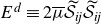 $E^{d} \equiv 2\overline {\mu } \widetilde {{\mathcal{S}}_{\textit{ij}}}\widetilde {{\mathcal{S}}_{\textit{ij}}}$
being the mean dissipation,
 $\varepsilon _t \equiv 2\overline {\mu {\mathcal{S}}_{\textit{ij}}^{\prime \prime} {\mathcal{S}}_{\textit{ij}}^{\prime \prime}}$
the turbulent dissipation and
 $\theta \equiv \partial u_l/\partial x_l$
the dilatation. The differential operator is defined as
 \begin{equation} \overline {\rho \frac{\textrm{D}}{\textrm{D}t}} \equiv \overline {\rho } \frac{\partial }{\partial t} + \overline {\rho }\widetilde {u}\frac{\partial }{\partial x} + \overline {\rho }\widetilde {v}\frac{\partial }{\partial y}. \end{equation}
In the framework of the Reynolds analogy, the key hypothesis is that the averaged enthalpy is a function of averaged velocity, i.e.
 $\widetilde {h} = \widetilde {h} ( \widetilde {u} )$
. The differential operator obeys the chain rule
 \begin{equation} \displaystyle \overline {\rho \frac{\textrm{D}}{\textrm{D}t}} \widetilde {h} = \frac{{\textrm{d}} \widetilde {h}}{{\textrm{d}} \widetilde {u}} \left ( \overline {\rho \frac{\textrm{D}}{\textrm{D}t}} \widetilde {u} \right )\!. \end{equation}
Substituting (3.2) and (3.3) into (3.5), one obtains
 \begin{equation} \begin{aligned} \frac{\partial \overline {p}}{\partial t} &+ \frac{\partial }{\partial x}\left ( \overline {\frac{\kappa }{C_{\!p}} \frac{\partial h}{\partial x}} - \overline {\rho } \widetilde {\ h^{\prime \prime}u^{\prime \prime}} \right ) + \frac{\partial \overline {up}}{\partial x} + \frac{\partial \overline {vp}}{\partial y} \\ & + \frac{\partial }{\partial y}\left ( -\overline {\rho } \widetilde {\ h^{\prime \prime}v^{\prime \prime}} + \overline {\frac{\kappa }{C_{\!p}} \frac{\partial h}{\partial y}} \right ) + E^d + 4\widetilde {{\mathcal{S}}_{\textit{ij}}} \overline {\mu {\mathcal{S}}_{\textit{ij}}^{\prime \prime}}+\varepsilon _t-\frac{2}{3}\overline {\mu \theta ^2} \\ &= \frac{{\textrm{d}} \widetilde {h}}{{\textrm{d}} \widetilde {u}} \left [ \frac{\partial }{\partial x} \left ( -\overline {p} + \overline { \sigma _{11}} -\overline {\rho } \widetilde {u^{\prime \prime} u^{\prime \prime}} \right ) + \frac{\partial }{\partial y} \left ({ -\overline {\rho }\widetilde {\ u^{\prime \prime}v^{\prime \prime}} } + \overline {\mu \frac{\partial v}{\partial x}} +\overline {\mu \frac{\partial u}{\partial y}} \right ) + \overline {\rho }\widetilde {f}_1 - \overline {\rho }\widetilde {\varphi }_1 \right ]\!. \end{aligned} \end{equation}
It is worth noting that (3.6) can be applied to any type of particle-laden wall-bounded turbulent flows. Nevertheless, this study is restricted to fully developed CTCFs, which will allow for a massive simplification of (3.6).
In a fully developed CTCF, the averaged physical quantities are statistically steady, e.g. the temporal variation of averaged pressure is zero. In addition, the continuity equation yields
 $\widetilde {v} = 0$
in fully developed CTCF. According to Pope (Reference Pope2000), the turbulent-viscosity hypothesis is valid if the anisotropy of Reynolds stress is locally determined by the mean strain rate. However, this condition is not generally satisfied by any type of turbulent flows. Fortunately, the turbulence characteristics and mean velocity gradient evolve slowly in turbulent channel flows, and therefore the turbulent-viscosity hypothesis is approximately valid. The Reynolds stress and Reynolds heat flux can be modelled by turbulent eddy viscosity and turbulent eddy conductivity as
 \begin{align} -\bar {\rho } \widetilde {u^{\prime \prime} v^{\prime \prime}} & = \bar {\mu }_t \frac{\partial \widetilde {u}}{\partial y}, \end{align}
 \begin{align} -\bar {\rho } \widetilde {h^{\prime \prime} v^{\prime \prime}} & = \frac{\bar {\kappa }_t}{C_{\!p}} \frac{\partial \widetilde {h}}{\partial y}. \end{align}
The validity of the turbulent-viscosity hypothesis also implies the local balance between turbulence production by the mean shear and the local processes such as kinetic energy redistribution and dissipation in the equations of Reynolds stress. To be specific, the turbulence dissipation is approximately balanced by the turbulence production in the outer layer of turbulent channel flows, i.e.
 \begin{equation} \varepsilon _t \approx {\mathcal{P}} = -\overline {\rho} {\widetilde{u^{\prime \prime}v^{\prime \prime}}} \frac{\partial {\widetilde{u}}}{\partial y}. \end{equation}
It is argued that the energy dissipation caused by dilation is negligible in CTCFs (Huang et al. Reference Huang, Coleman and Bradshaw1995). As a result, the mean energy dissipation in fully developed turbulent channel flow can be rewritten as
 \begin{equation} E^d \approx 2\overline {\mu } \left (\frac{\partial \widetilde {u}}{\partial x}\right )^2 + \overline {\mu } \left ( \frac{\partial \widetilde {u}}{\partial y}\right )^2. \end{equation}
In a CTCF driven by constant body force, there are no density and pressure gradients along streamwise direction when the flow reaches a fully developed state (Huang et al. Reference Huang, Coleman and Bradshaw1995). All physical variables are purely a function of distance to the wall. Besides, the contribution of
 $\overline {u^{\prime \prime}}$
and
 $\overline {h^{\prime \prime}}$
is relatively very small compared with
 $\widetilde {u}$
and
 $\widetilde {h}$
(Huang et al. Reference Huang, Coleman and Bradshaw1995). By combining the above-described modelling and approximations, (3.6) can be simplified to
 \begin{equation} \begin{aligned} \frac{{\textrm{d}} \overline {v^{\prime \prime} p}}{{\textrm{d}} y} &+ \frac{{\textrm{d}} }{{\textrm{d}} y}\left ( \frac{\overline {\kappa } + \overline {\kappa }_t}{C_{\!p}} \frac{{\textrm{d}} \widetilde {h}}{{\textrm{d}} y} \right ) + (\overline {\mu } + \overline {\mu }_t) \left ( \frac{{\textrm{d}} \widetilde {u}}{{\textrm{d}} y}\right )^2 = \\ & \frac{{\textrm{d}} \widetilde {h}}{{\textrm{d}} \widetilde {u}} \left [ \frac{{\textrm{d}}}{{\textrm{d}} y} \left ( (\overline {\mu }+\overline {\mu }_t)\frac{{\textrm{d}} \widetilde {u}}{{\textrm{d}} y} \right ) + \overline {\rho }\widetilde {f}_1 - \bar {\rho }\widetilde {\varphi }_1 \right ]\!. \end{aligned} \end{equation}
Let
 $\tau$
denote the total shear stress and
 ${\textit{Pr}}_m$
the mixed Prandtl number, which are, respectively, defined as
 \begin{align} \tau &= (\overline {\mu }+\overline {\mu }_t)\frac{{\textrm{d}} \widetilde {u}}{{\textrm{d}} y}, \end{align}
 \begin{align} \textit{Pr}_m &= C_{\!p}\frac{\overline {\mu }+\overline {\mu }_t}{\overline {\kappa }+\overline {\kappa }_t}. \end{align}
Then, (3.11) is reformulated to
 \begin{eqnarray} \frac{{\textrm{d}}}{{\textrm{d}} \widetilde {u}}\left ( \frac{\tau }{\textit{Pr}_m} \frac{{\textrm{d}} \widetilde {h}}{{\textrm{d}} \widetilde {u}} \right ) - \frac{{\textrm{d}} \widetilde {h}}{{\textrm{d}} \widetilde {u}} \frac{{\textrm{d}} \tau }{{\textrm{d}} \widetilde {u}} +\tau = \left ( \frac{{\textrm{d}} \widetilde {u}}{{\textrm{d}} y}\right )^{-1} \left [ \frac{{\textrm{d}} \widetilde {h}}{{\textrm{d}} \widetilde {u}} \left ( \overline {\rho }\widetilde {f}_1 - \bar {\rho }\widetilde {\varphi }_1 \right ) - \frac{{\textrm{d}} \overline {v^{\prime \prime} p}}{{\textrm{d}} y} \right ] \end{eqnarray}
by applying again the chain rule of differentiation. The left-hand side of (3.14) is the same as the van Driest equation given by van Driest (Reference van Driest1955), which reflects the similarity between the evolutions of
 $\widetilde {u}$
and
 $\widetilde {h}$
. By contrast, the first two terms on the right-hand side of (3.14) are additional source terms to the van Driest equation caused by the pressure gradient and particle feedback effects, which are balanced by the total stress. The last term can be represented by enthalpy using the equation of state for an ideal gas and the relation between temperature and enthalpy. Thus, the last term on the right-hand side of (3.14) is reformulated as
 $\overline {v^{\prime \prime} p } = r_0 \overline {\rho v^{\prime \prime}T} = (r_0/C_{\!p} ) \overline {\rho } \widetilde {\ v^{\prime \prime} h} = (r_0/C_{\!p}) \overline {\rho } \widetilde {\ v^{\prime \prime} h^{\prime \prime}}$
. With the thermodynamic condition
 $r_0 = C_{\!p} - C_V$
and
 $\gamma = C_{\!p}/C_V$
, the source term is denoted by
 $S^{hu}$
and expressed as
 \begin{align} S^{hu} = \left ( \frac{{\textrm{d}} \widetilde {u}}{{\textrm{d}} y}\right )^{-1} \left [ -\frac{{\textrm{d}} \widetilde {h}}{{\textrm{d}} \widetilde {u}} \frac{{\textrm{d}} \tau }{{\textrm{d}} y } - \frac{\gamma - 1}{\gamma } \frac{{\textrm{d}} \overline {\rho } \widetilde {\ v^{\prime \prime} h^{\prime \prime}}}{{\textrm{d}} y} \right ]\!. \end{align}
To evaluate the contribution of
 $S^\textit{hu}$
to (3.14), it is compared with the only zero-order term on the left-hand side of (3.14), i.e.
 $\tau$
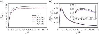
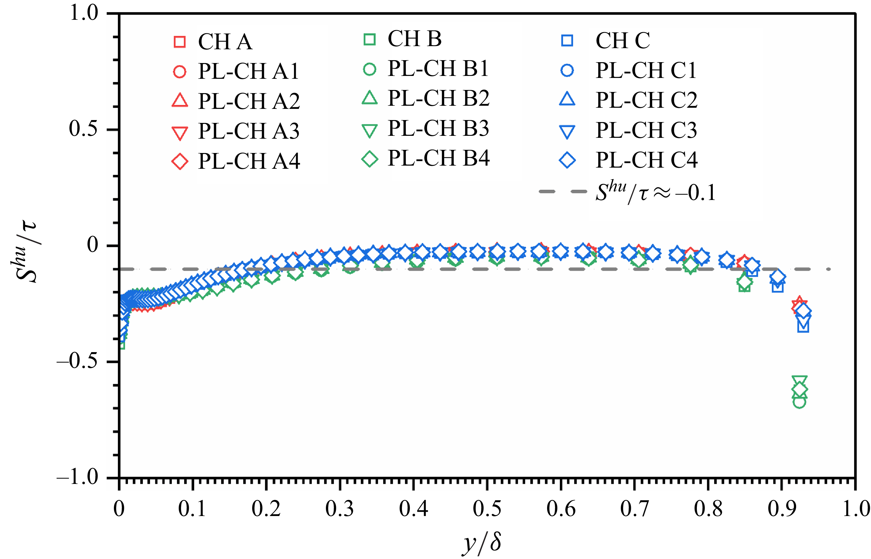
. Depicted in figure 3 are the distributions of
 $S^{hu}/\tau$
against the distance to the wall extracted from DNS data of single-phase CTCFs and particle-laden CTCFs. The numerical results reveal that the ratio of
 $S^{hu}$
to
 $\tau$
is very small (
 $|S^{hu}/\tau | \lesssim 0.1$
) within the region between
 $y/\delta \gt 0.15$
and
 $y/\delta \lt 0.85$
, which occupies the majority of channel. Thus, the contribution of
 $S^{hu}$
to (3.14) is negligible compared with the total stress for both single-phase and particle-laden CTCFs. It should be emphasized that the neglect of
 $S^{hu}$
with respect to
 $\tau$
is only valid in the parameter range of present simulations, i.e. small particles with moderate particle inertia and relatively moderate particle mass fraction.
Profiles of the normalized source term (3.15):
 $S^{hu}/\tau$
. The distance to the wall
 $y$
is normalized by the half-width of the channel
 $\delta$
. Numerical results for both single-phase CTCFs and particle-laden CTCFs are plotted for comparison.
As a result, (3.14) degenerates to a similar form to that in turbulent boundary layer with zero pressure gradient and isothermal wall condition
 \begin{equation} \frac{{\textrm{d}}}{{\textrm{d}} \widetilde {u}}\left ( \frac{\tau }{\textit{Pr}_m} \frac{{\textrm{d}} \widetilde {h}}{{\textrm{d}} \widetilde {u}} \right ) - \frac{{\textrm{d}} \widetilde {h}}{{\textrm{d}} \widetilde {u}} \frac{{\textrm{d}} \tau }{{\textrm{d}} \widetilde {u}} + \tau = 0, \end{equation}
which is first given by van Driest (Reference van Driest1955). Up to now, the work of van Driest has been successfully extended to particle-laden CTCFs. Before solving (3.16), it is worth addressing that the establishment of the van Driest equation presented herein can also be applied to any other kind of fully developed internal wall-bounded turbulent flow, such as turbulent pipe flow. However, the direct application of this methodology to the turbulent boundary layer with non-zero pressure gradient is impossible. It is expected that the methodology and analysis procedure presented in this paper might inspire similar research in particle-laden turbulent boundary layers with non-zero pressure gradient.
Returning back to the current research regarding CTCFs, the remaining work is to solve (3.16). The detailed steps for solving this equation are given in Fernholz & Finley (Reference Fernholz and Finley1980). We only provide readers with the most important ingredients herein. Instead of directly solving (3.16), it is suggested to deal with a non-dimensionalized equation by normalizing the averaged velocity
 $\widetilde {u}$
with its value at the central plane
 $u_c$
, the averaged enthalpy
 $\widetilde {h}$
with its value at the same position
 $h_c$
and the total shear stress
 $\tau$
with the wall shear stress
 $\tau _w$
. Let
 $h^*$
,
 $u^*$
and
 $\tau ^*$
denote, respectively, the non-dimensionalized variables, and then (3.16) is rewritten as
 \begin{equation} \tau ^* \left [ \frac{{\textrm{d}}}{{\textrm{d}} u^*}\left ( \frac{1}{\textit{Pr}_m} \frac{{\textrm{d}} h^*}{{\textrm{d}} u^*}\right ) + \frac{u_c^2}{h_c} \right ] + \frac{1-{\textit{Pr}}_m}{\textit{Pr}_m} \frac{{\textrm{d}} h^*}{{\textrm{d}} u^*} \frac{{\textrm{d}} \tau ^*}{{\textrm{d}} u^*} = 0, \end{equation}
with the boundary condition
 $h^*(1) = 1$
. By the way, the normalized enthalpy
 $h^*$
and temperature
 $T^* = T/T_c$
(with
 $T_c$
being the Favre-averaged temperature at the central plane) are exactly equal to each other. Therefore,
 $h^*$
can be replaced by
 $T^*$
. The solution to (3.17) is
 \begin{align} T^* &= T^*(0) + \left [ 1-T^*(0) \right ] \frac{S(u^*)}{s} + \frac{u_c^2}{C_{\!p} T_c} \frac{r}{2} \left [ \frac{S(u^*)}{s} - \frac{2R(u^*)}{r} \right ]\!, \end{align}
 \begin{align} S(u^*) &= \int _0^{u^*} {\textit{Pr}}_m \exp \left ( \int _{1}^{\tau ^*} \frac{\textit{Pr}_m-1}{\tau } {\textrm{d}} \tau \right ) {\textrm{d}}u, \end{align}
 \begin{align} R(u^*) &= \int _0^{u^*} {\textit{Pr}}_m \exp \left ( \int _{1}^{\tau ^*} \frac{\textit{Pr}_m-1}{\tau } {\textrm{d}} \tau \right ) \int _0^{u} \exp \left ( \int _1^{\tau ^*} \frac{1- {\textit{Pr}}_m}{\tau } {\textrm{d}} \tau \right ) {\textrm{d}}u {\textrm{d}}u, \end{align}
with
 $s = S(1)$
being the Reynolds analogy factor and
 $r = 2R(1)$
the recovery factor. It is very difficult (or nearly impossible) to look for an analytical expression for
 $S(u^*)$
and
 $R(u^*)$
. Walz (Reference Walz1969) tried to numerically determine
 $S(u^*)$
and
 $R(u^*)$
by varying the Prandtl number. Although the Prandtl number will influence the results of
 $S(u^*)$
and
 $R(u^*)$
, Walz (Reference Walz1969) still suggests that
 $S(u^*)/s \approx u^*$
and
 $2R(u^*)/r \approx {u^*}^2$
, which lead to the famous Walz’s equation
 \begin{equation} \begin{aligned} \frac{\widetilde {T}}{T_c} &= \frac{T_w}{T_c} + \frac{T_c-T_w}{T_c} \frac{\widetilde {u}}{u_c} + \frac{u_c^2}{C_{\!p} T_c} \frac{r}{2} \left [ \frac{\widetilde {u}}{u_c} - \left (\frac{\widetilde {u}}{u_c}\right )^2 \right ] \\ &= \frac{T_w}{T_c} + \frac{T_{rc}-T_w}{T_c} \frac{\widetilde {u}}{u_c} + \frac{T_c - T_{rc}}{T_c} \left (\frac{\widetilde {u}}{u_c}\right )^2 , \end{aligned} \end{equation}
with
 $T_{rc} \equiv T_c + r u_c^2/(2C_{\!p})$
being the recovery temperature at the central plane. In what follows, we will examine these approximations first in single-phase CTCFs and then in particle-laden CTCFs.
3.2. Reynolds analogy in single-phase CTCF
The mixed Prandtl number is of great significance in the Reynolds analogy as it is the sole variable coefficient in (3.17). It can be seen that the mixed Prandtl number has a decisive impact on both
 $S(u^*)$
and
 $R(u^*)$
. The profile of
 ${\textit{Pr}}_m$
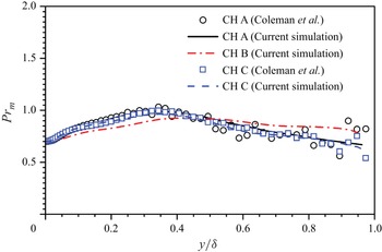
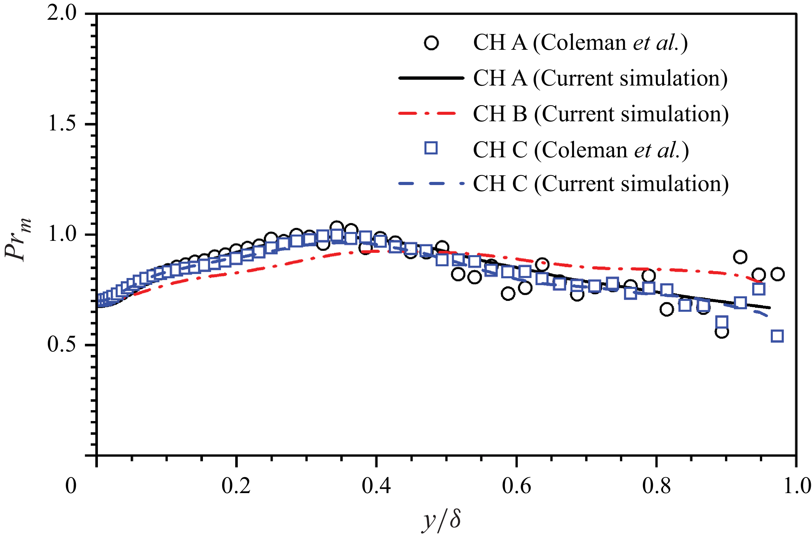
plays a very important role in determining the solution given in (3.18). Therefore, it is necessary to validate the profile of mixed Prandtl number computed in this study. Depicted in figure 4 are the profiles of
 ${\textit{Pr}}_m$
along wall-normal direction. The numerical results of the current simulation agree well with those given by Coleman et al. (Reference Coleman, Kim and Moser1995) in the near-wall region. It is observed that the data reported in the literature oscillate around the curves obtained in the present simulation, especially in the outer-layer regions of the channel, which also validates the present numerical simulations.
Profiles of the mixed Prandtl number obtained in cases CH A (black solid line), CH B (red dash–dotted line) and CH C (blue dashed line). The corresponding profiles reported by Coleman et al. (Reference Coleman, Kim and Moser1995) for cases CH A and CH C are also plotted for comparison (see circles and squares, respectively).
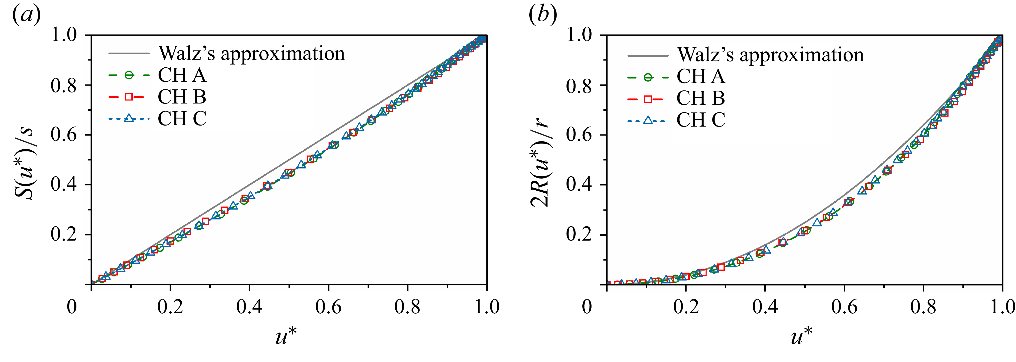
Profiles of (a)
 $S(u^*)/s$
and (b)
 $2R(u^*)/r$
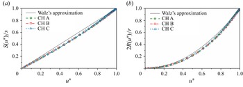
obtained in cases CH A, CH B and CH C. The Walz approximations are also included for comparison.
With reliable profiles of
 ${\textit{Pr}}_m$
, the numerical integration gives the profiles of
 $S(u^*)/s$
as shown in figure 5(a). It appears that all test cases CH A, CH B and CH C present similar profiles of
 $S(u^*)/s$
. However, these profiles deviate from Walz’s approximation for
 $S(u^*)/s \approx u^*$
. It is believed that this deviation finally results in the failure of Walz’s equation in predicting the temperature–velocity relation in CTCFs as demonstrated by Zhang et al. (Reference Zhang, Bi, Hussain and She2014). In fact, Walz’s approximation (Walz Reference Walz1969)
 $S(u^*)/s \approx u^*$
is based on two assumptions, i.e.
 ${\textit{Pr}}_m$
is constant and the total shear stress satisfies the Blasius profile. According to the first assumption, (3.19) is equivalent to
 \begin{equation} S(u^*) = {\textit{Pr}}_m \int _{0}^{u^*} {\tau ^*}^{\textit{Pr}_m - 1} {\textrm{d}} u. \end{equation}
With the laminar Blasius approximation (Blasius Reference Blasius1908)
 $\tau ^* \approx 1 - {u^*}^{3.5}$
, one can finally obtain
 $S$
as a function of
 $u^*$
. It is obvious that neither of those two assumptions holds for CTCF. Therefore, a correction function
 $\alpha (u^*)$
is introduced in this work to consider the effect of non-uniform mixed Prandtl number and total shear in CTCFs, i.e.
 $S(u^*)/s = (1-\alpha (u^*) )u^*$
. Before the determination of a specific form of
 $\alpha$
, an attempt is first made to evaluate the form of
 $R(u^*)/r$
. If
 $S(u^*) \sim (1-\alpha (u^*) )u^*$
, one can readily reach
 \begin{equation} {\textit{Pr}}_m \exp \left ( \int _{1}^{\tau ^*} \frac{\textit{Pr}_m-1}{\tau } {\textrm{d}} \tau \right ) {\textrm{d}} u \sim 1 - (\dot {\alpha } u^* + \alpha ), \end{equation}
where
 $\dot {\alpha }$
represents the derivative of
 $\alpha$
with respect to
 $u^*$
. By substituting (3.23) into the definition of
 $R(u^*)$
given in (3.20), one gets
 \begin{equation} R(u^*) \sim \int _0^{u^*} 1 - (\dot {\alpha } u + \alpha ) \int _0^{u} \frac{1}{1 - (\dot {\alpha } u + \alpha )} {\textrm{d}} u {\textrm{d}} u \approx {u^*}^2 \end{equation}
by neglecting high-order terms of
 $\alpha$
and terms of a degree higher than
 ${u^*}^2$
. The former approximation is based on the observation that the deviation presented in figure 5(a) is relatively small, which means
 $\alpha \ll 1$
. The latter is owing to the fact that
 $u^* \leqslant 1$
. Although figure 5(b) suggests that this approximation may not be totally accurate, it is believed that the numerical results are close enough to Walz’s approximation. Besides, it is supposed that the major factor in the Reynolds analogy modelling is
 $S(u^*)$
rather than
 $R(u^*)$
. Therefore, Walz’s approximation for
 $R(u^*)$
is retained in what follows.
In order to determine a specific form of the correction function
 $\alpha$
, one first needs to impose its boundary values. By definition, the value of
 $\alpha (u^*)$
at the central plane can be easily obtained, i.e.
 $\alpha (1)=0$
. Meanwhile, the heat flux at the wall gives an estimation of
 $\alpha (0)$
by the relation
 \begin{equation} -\! \textit{Pr}\frac{u_c q_w}{C_{\!p} T_c \tau _w}=\frac{{\textrm{d}} T^*}{{\textrm{d}} u^*}(0) = \left [ 1 - T^*(0) + \frac{u_c^2}{C_{\!p} T_c}\frac{r}{2} \right ] \left [ 1-\alpha (0) \right ]\!, \end{equation}
which leads to
 \begin{equation} \alpha (0) = 1 + \textit{Pr} \frac{u_c q_w}{C_{\!p} (T_{rc} - T_w) \tau _w} = 1 - s \textit{Pr}. \end{equation}
Here,
 \begin{equation} s = - \frac{u_c q_w}{C_{\!p} (T_{rc}-T_w) \tau _w} \end{equation}
is the commonly used Reynolds analogy factor in wall-bounded turbulent flows (Wenzel et al. Reference Wenzel, Gibis, Kloker and Rist2021), which is capable of characterizing the overall effect of the Reynolds analogy.
Up to now, the boundary values of
 $\alpha$
have been prescribed. The last missing piece is the profile of
 $\alpha$
. An asymptotic analysis gives that
 $\alpha (u^*) = \alpha (0) (1-{u^*}^{\beta })$
, which satisfies the two aforementioned boundary conditions. It should be mentioned that the value of
 $\beta$
remains unknown theoretically. The numerical results reveal that
 $\beta$
can be taken as
 $4/3$
for all the single-phase turbulent channel flows under consideration in this study. However, it is noteworthy that the new model can successfully retrieve the generalized Reynolds analogy (GRA) model proposed by Zhang et al. (Reference Zhang, Bi, Hussain and She2014) when
 $\beta$
is set to 1:
 \begin{equation} \begin{aligned} \frac{\widetilde {T}}{T_c} &= \frac{T_w}{T_c} + \frac{T_c-T_w}{T_c}(1-\alpha ) \frac{\widetilde {u}}{u_c} + \frac{u_c^2}{C_{\!p} T_c} \frac{r}{2} \left [(1-\alpha ) \frac{\widetilde {u}}{u_c} - \left (\frac{\widetilde {u}}{u_c}\right )^2 \right ] \\ &= \frac{T_w}{T_c} + \frac{T_{rc}-T_w}{T_c} \frac{\widetilde {u}}{u_c} \left [ (1-{\boldsymbol{sPr}})\left (1-\frac{\widetilde {u}}{u_c}\right ) \right ] + \frac{T_c - T_{rc}}{T_c} \left (\frac{\widetilde {u}}{u_c}\right )^2 \\ & = \frac{T_w}{T_c} + \frac{T_{rc}-T_w}{T_c}\left [ (1-{\boldsymbol{sPr}})\left (\frac{\widetilde {u}}{u_c}\right )^2 + {\boldsymbol{sPr}} \frac{\widetilde {u}}{u_c} \right ] + \frac{T_c - T_{rc}}{T_c} \left (\frac{\widetilde {u}}{u_c}\right )^2 . \end{aligned} \end{equation}
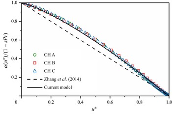
However, the linear approximation seems not to be rigorous enough. Displayed in figure 6 are profiles of the correction function normalized by its value at the wall. The numerical results are clearly not a linear profile, which makes the approximation in GRA questionable. In this paper, we suggest an empirical value for the power exponent
 $\beta \approx 4/3$
for single-phase CTCFs, which is also plotted in figure 6. It demonstrates that this value could better fit the correction functions obtained by using DNS data. Consequently, a new model is proposed as
 \begin{align} T^* = T^*(0) &+ \left [ 1-T^*(0) \right ] \left [1-\alpha (u^*)\right ] u^* + \frac{u_c^2}{C_{\!p} T_c} \frac{r}{2} \left [ \left [1-\alpha (u^*)\right ] u^* - {u^*}^2 \right ]\!, \end{align}
 \begin{align} &\qquad\qquad\quad \alpha (u^*) = (1-{\boldsymbol{sPr}}) (1-{u^*}^{\beta }). \end{align}
Profiles of
 $\alpha /\alpha (0)$
obtained in cases CH A, CH B and CH C (symbols). The approximation model proposed by Zhang et al. (Reference Zhang, Bi, Hussain and She2014) and that given in present paper (3.30) are plotted as dashed and solid lines, respectively.
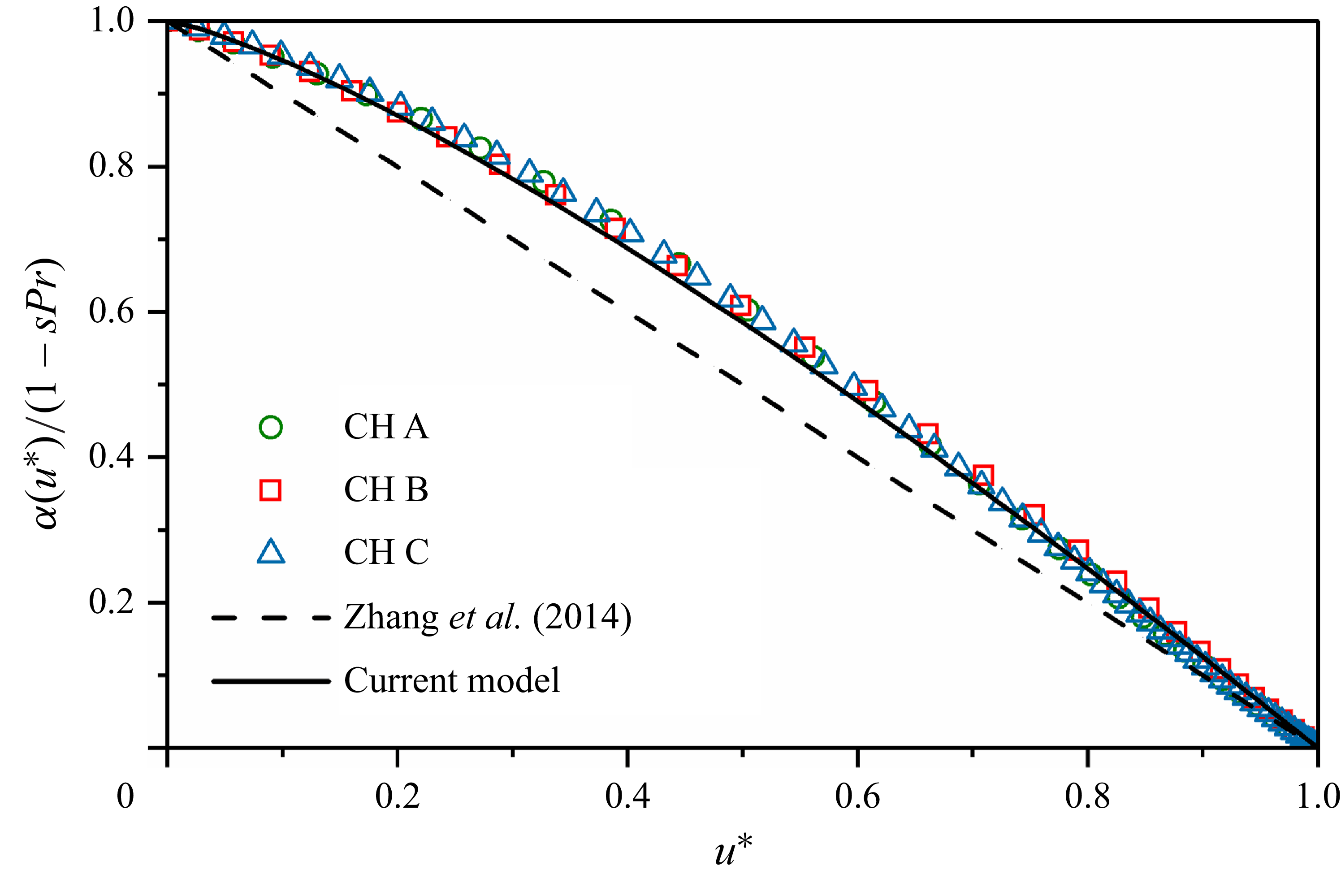
The new correction function agrees very well with the numerical observations as shown in figure 6. Besides, it can be seen that
 $\alpha (0)$
contains other flow parameters such as the Reynolds analogy factor (
 $s$
) and the Prandtl number (
 ${\textit{Pr}}$
). It requires more DNS data in a wider range of parameters to study the influence of flow parameters on
 $\beta$
, and as a result, on
 $\alpha$
, which is left for further investigation.
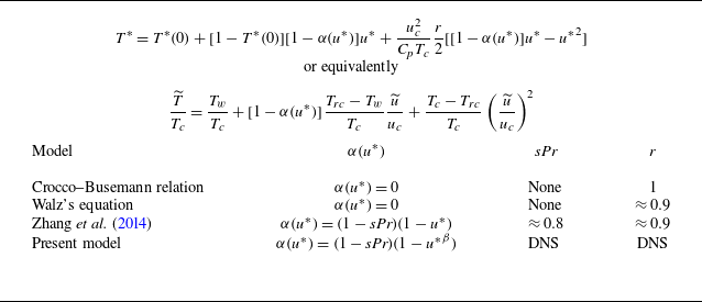
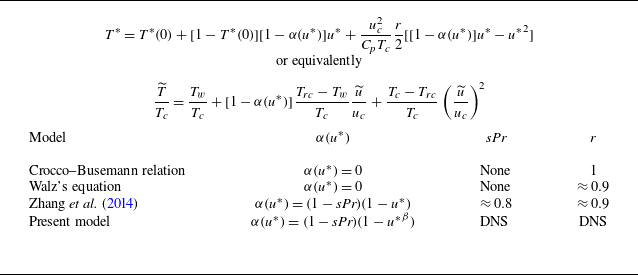
Summary of different models for temperature–velocity relation.
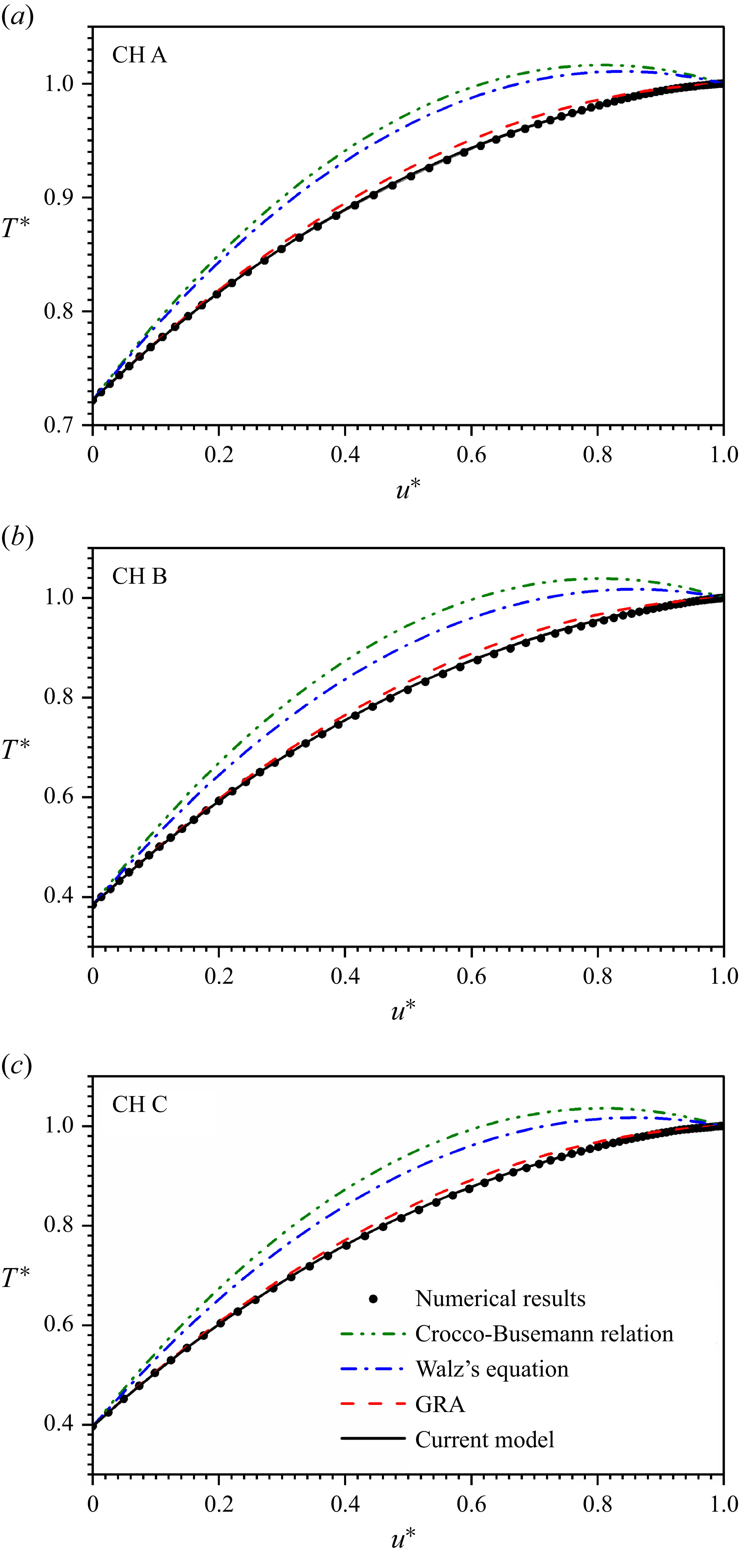
Temperature–velocity profiles obtained from present DNS data (symbols): (a) CH A, (b) CH B and (c) CH C. The analytical models given by Crocco–Busemann relation (dash–dot–dotted lines), Walz’s equation (dash–dotted lines), GRA (dashed lines) and present model (3.29) (solid lines) are included for comparison.
Before discussing the discrepancies, different temperature–velocity relations are summarized in table 3 along with the parameters employed in each model. Apart from the three models examined in this paper, the Crocco–Busemann relation is also included for comparison. There are three aspects affecting the performance of a model, i.e. the correction function
 $\alpha (u^*)$
, the product of Prandtl number and Reynolds analogy factor
 ${\boldsymbol{sPr}}$
, and the recovery factor
 $r$
. In the Crocco–Busemann relation, the total temperature, i.e.
 $r=1$
, is used instead of recovery temperature. Besides, there is no correction function in the Crocco–Busemann relation. The improvement of Walz’s equation compared with the Crocco–Busemann relation is the employment of recovery temperature with the recovery factor
 $r \approx 0.9$
. As for GRA and present model, the correction function is included and the effect of wall heat flux is no longer left aside. The correction function in GRA is linear, while the present model obeys a power law of
 $1.27$
. The factors
 ${\boldsymbol{sPr}}$
and
 $r$
in GRA take the recommended values. By contrast, their values are numerically computed in the present model. A detailed discussion regarding
 ${\boldsymbol{sPr}}$
and
 $r$
is given in § 3.3. Figure 7 displays the comparison between DNS results and different theoretical models. It can be observed that the absence of a correction function (e.g. the Crocco–Busemann relation and Walz’s equation) shows poor agreement with the DNS results. As expected, the correction function improves massively the model quality. Although both GRA and the present model can reproduce the DNS results, the new model exhibits an advantage in the near-wall regions.
The power exponent
 $\beta$
in the correction function (3.30) with respect to Stokes number
 $St$
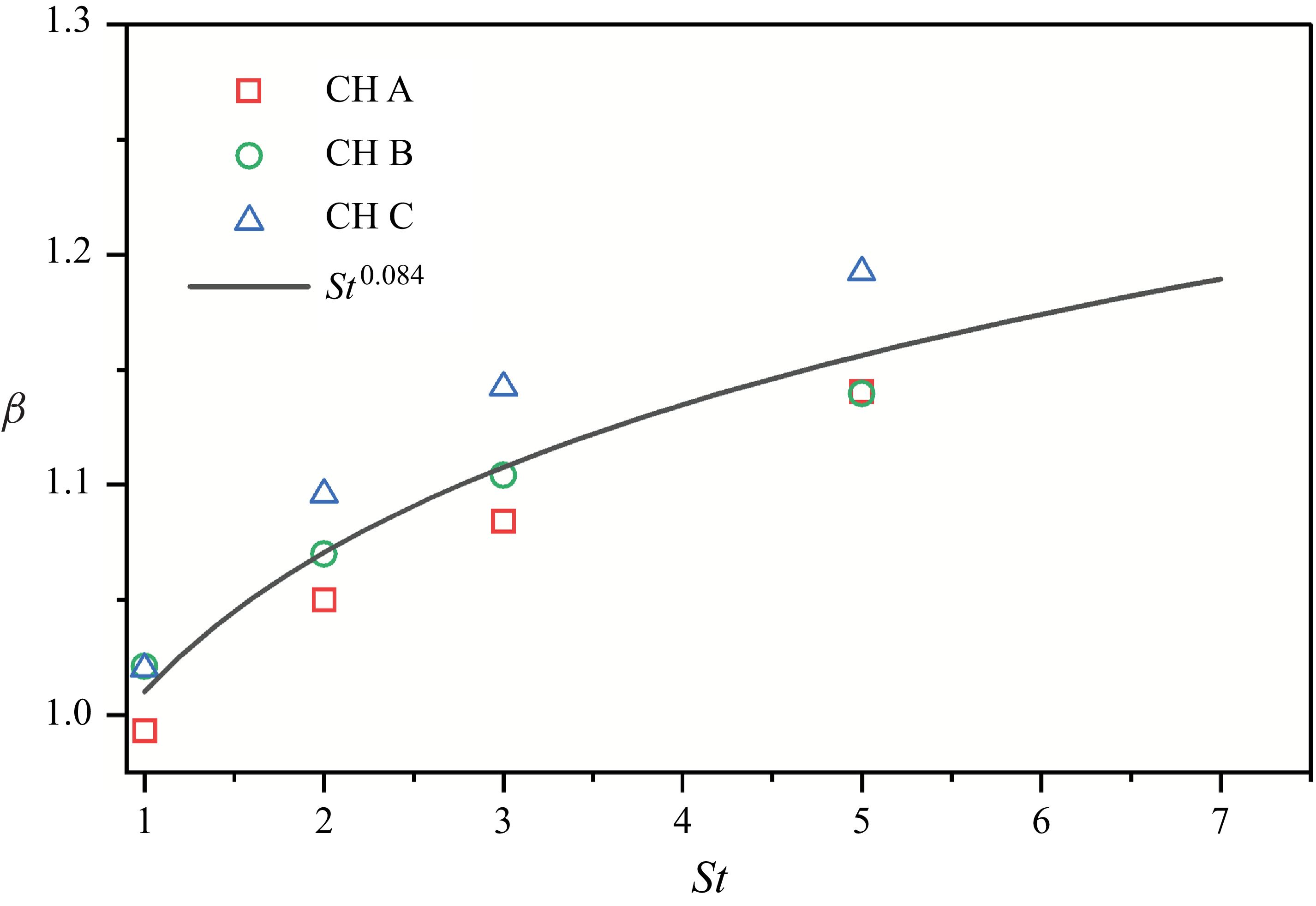
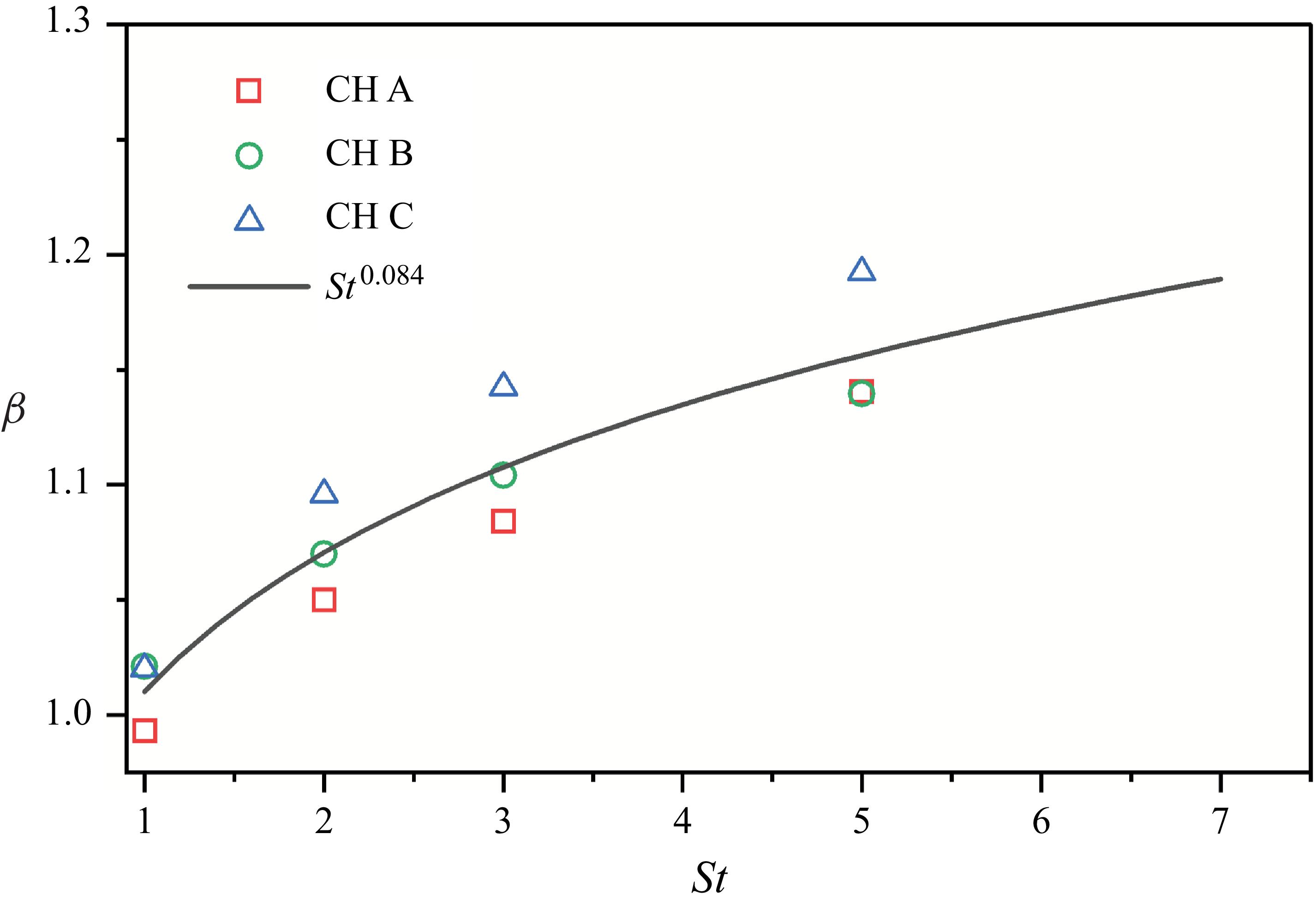
for particle-laden CTCFs. The data fitted power law approximation relation is plotted as a solid line. Different background flows are marked by various symbols: (a) CH A, (b) CH B and (c) CH C.
3.3. Application to particle-laden CTCF
With the temperature–velocity relation (3.29) established and validated in single-phase CTCFs, it can be now applied to particle-laden CTCFs. Unlike their single-phase counterpart, the power exponent in the correction function
 $\beta$
is smaller than that in single-phase CTCFs as shown in figure 8. It is manifested from figure 8 that
 $\beta$
increases with the particle Stokes number. The influences of Reynolds and Mach numbers are less important than the particle Stokes number. The power exponent
 $\beta$
is supposed to be proportional to
 $St^{0.084}$
for the range of flow and particle parameters under consideration. The empirical relation
 \begin{equation} \beta \approx 1.01 St^ {0.084} \end{equation}
is employed to predict the mean temperature profiles for particle-laden CTCFs in what follows. It is clearly seen from figure 8 that
 $\beta$
increases with Stokes number, Reynolds number and Mach number. In fact, the exponent factor
 $\beta$
is dependent on the profiles of
 ${\textit{Pr}}_m$
and
 $\tau$
because the correction function
 $\alpha$
comes from the non-uniform mixed Prandtl number and total shear stress
 $\tau = (\mu + \mu _t) {\textrm{d}} \widetilde {u} / {\textrm{d}} y$
in turbulent flows. However,
 $\tau$
differs from the Blasius approximation in particle-laden flows since the particle feedback force contributes to the total shear balance. This difference is much more pronounced with the increases of Stokes number, Reynolds number and Mach number, which finally leads to the variation trend of
 $\beta$
with respect to these dimensionless parameters.
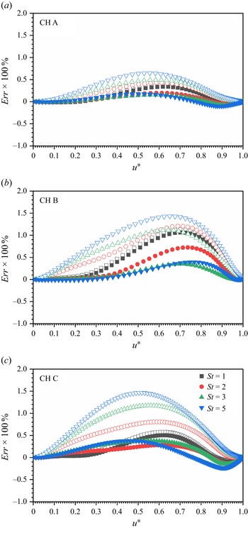
Relative error of mean temperature between the theoretical models and DNS data for particle-laden CTCFs. The open and solid symbols represent the results given by GRA and new model (3.29), respectively. Three carrier flows are marked by (a) CH A, (b) CH B and (c) CH C, respectively.
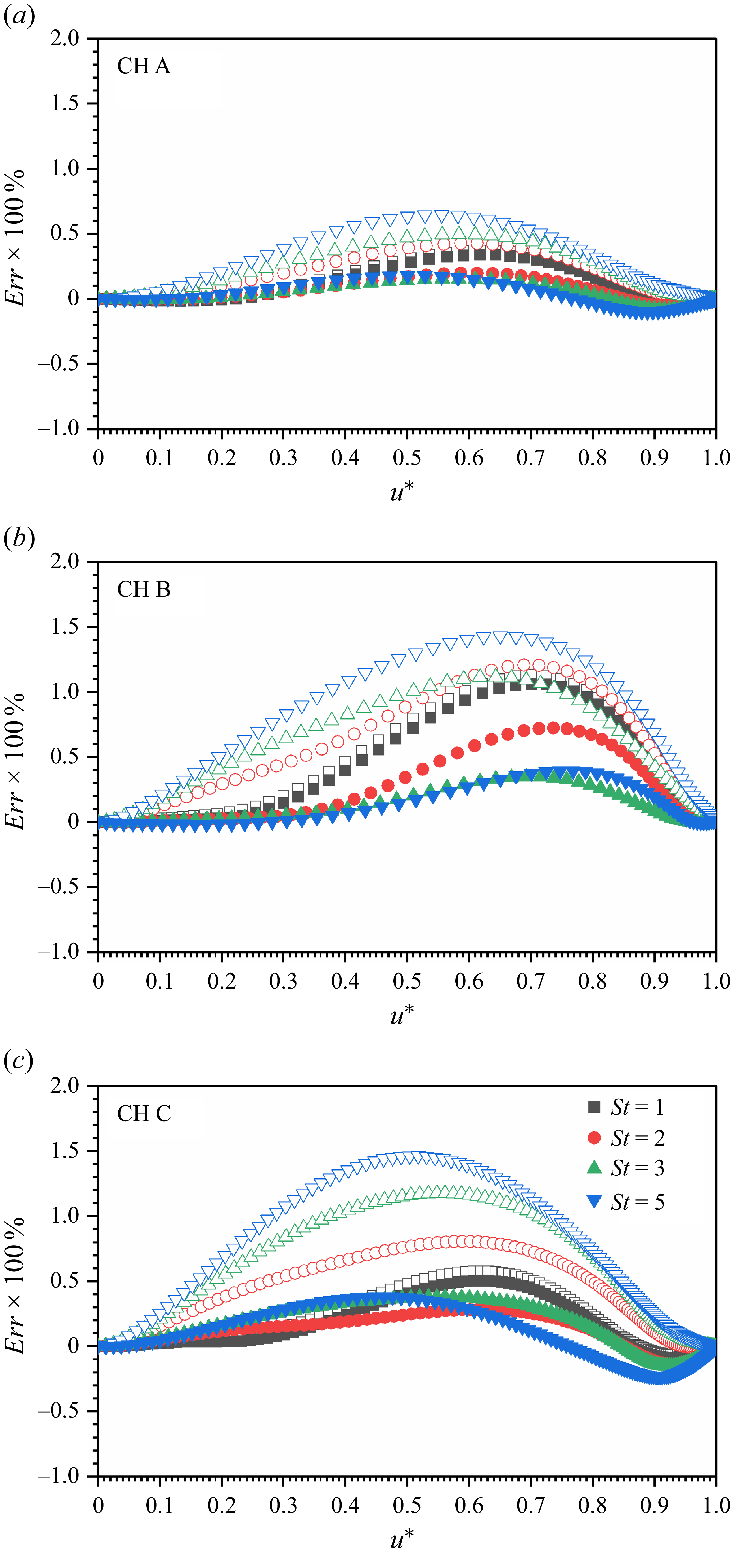
It is worth mentioning again that the physical implication of the new model lies in its importance for modelling of particle-laden flows. To compare our new model with GRA, the relative error of model-predicted temperature–velocity relation with respect to the DNS results is defined as
 $\textit{Err} = (T^*_{\textit{model}}-T^*_{\textit{DNS}})/T^*_{\textit{DNS}}$
. Displayed in figure 9 are the relative errors between theoretical models (GRA and the present model) and DNS results. The current model presents a very similar relative error for particle-laden CTCFs of
 $St = 1$
. This is because the power exponent
 $\beta$
is approximately
 $1$
for this case. The relative error of the GRA model given by Zhang et al. (Reference Zhang, Bi, Hussain and She2014) increases with the particle Stokes number, flow Reynolds number and Mach number. By contrast, an obvious improvement is observed for the new model in CTCFs laden with inertial particles even at large Stokes numbers. It turns out that the relative errors of the new model are all smaller than
 $0.5\,\%$
for different two-phase CTCHs. Therefore, it can be concluded that the new model is more accurate than the GRA, reducing the relative errors by approximately 50 %. It should be mentioned here that the success of both GRA and the present model also validates the theoretical analysis given in § 3.1.
Last but not least, the Reynolds analogy factor
 $s$
and recovery factor
 $r$
are two determining parameters in constructing a temperature–velocity relation in CTCFs. Therefore, special interests are addressed to their values herein. Zhang et al. (Reference Zhang, Bi, Hussain and She2014) suggest that
 $sPr \approx 0.8$
and
 $r \approx 0.9$
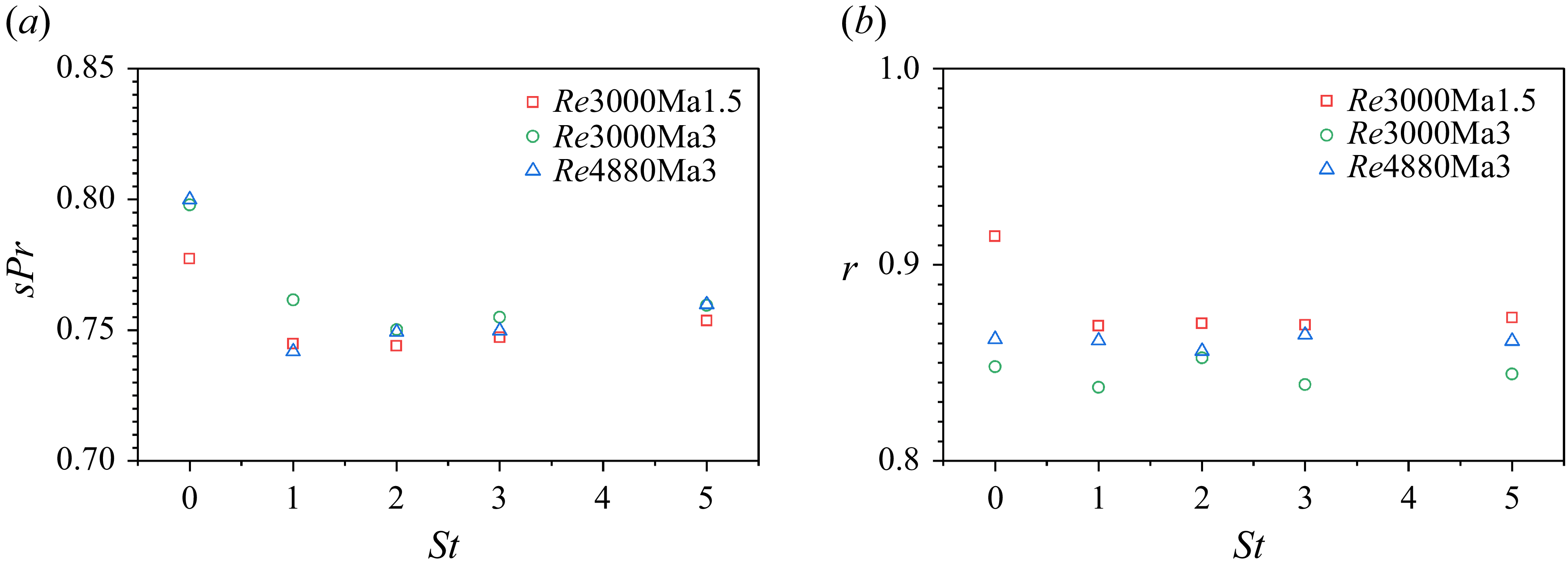
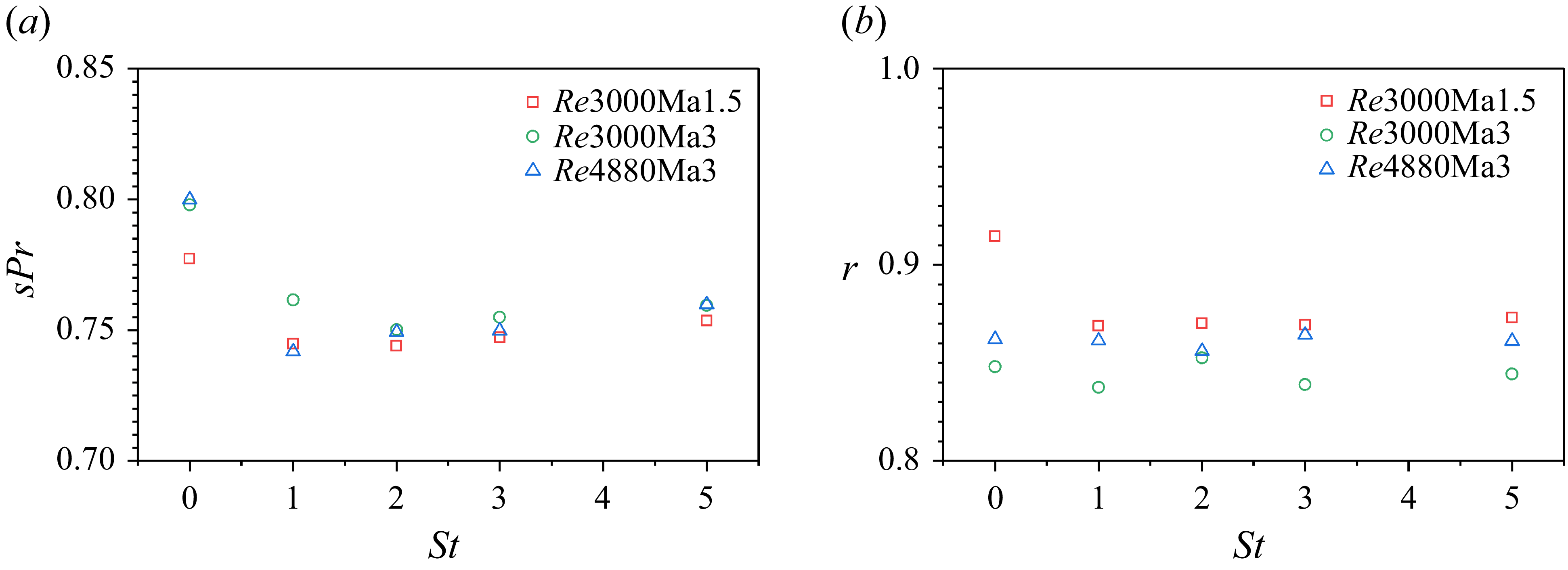
in single-phase CTCFs. By contrast, their values in particle-laden CTCFs are rarely reported. Depicted in figure 10 are the evolutions of
 ${\boldsymbol{sPr}}$
and
 $r$
with respect to the particle Stokes number, where the single-phase CTCFs correspond to
 $St=0$
. The factor
 ${\boldsymbol{sPr}}$
shows a strong dependency on particle Stokes number. The Reynolds analogy factor is first reduced by the inertial particles, and then starts to be augmented with particle Stokes number after reaching its minimal value. It is very interesting that the Reynolds analogy factor seems to be irrelevant to Reynolds and Mach numbers within the parameter range of this study, which suggests that a single-variable function is sufficient to describe the Reynolds analogy parameter. Different from
 ${\boldsymbol{sPr}}$
, the recovery factor is less sensitive to the particle Stokes number. It can be considered as constant except for the case of
 $St=0$
at
 ${\textit{Re}}_{\tau } = 220$
. Despite that, the recovery factor is over-estimated by Zhang et al. (Reference Zhang, Bi, Hussain and She2014). The present numerical results indicate that the values of
 $r$
fall within the range between
 $0.83$
and
 $0.87$
rather than take a specific value of
 $0.9$
.
(a) Rescaled Reynolds analogy factor
 ${\boldsymbol{sPr}}$
and (b) recovery factor
 $r$
against particle Stokes number for different carrier CTCFs. The values in single-phase CTCFs are also plotted with
 $St=0$
.
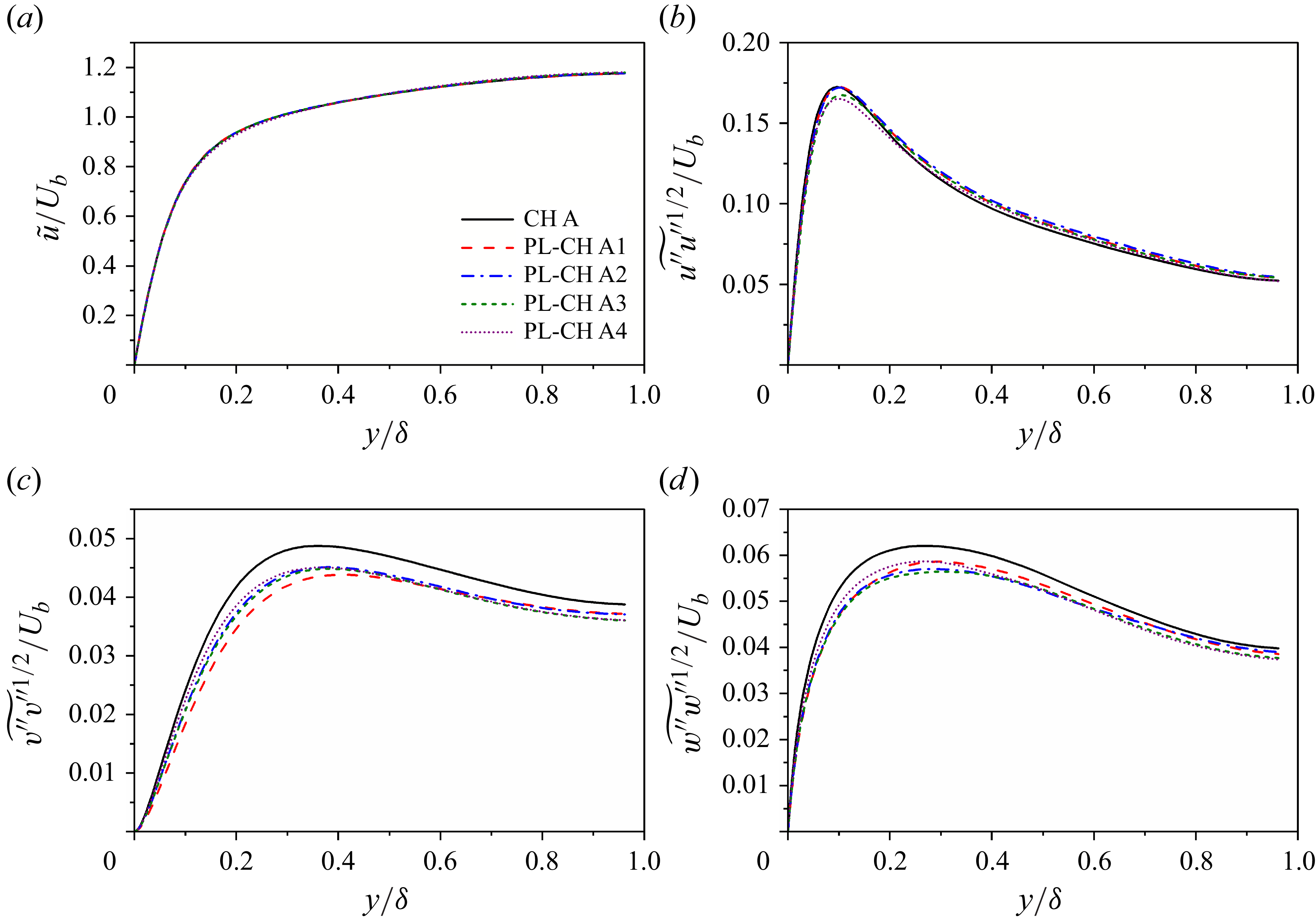
Profiles of (a) density-weighted mean velocity, r.m.s. density-weighted fluctuating velocities normalized by bulk velocity
 $U_b$
in (b) streamwise, (c) wall-normal and (d) spanwise directions for both clean and particle-laden CTCFs at
 ${\textit{Re}}=3000$
and
 ${\textit{Ma}}=1.5$
.
4. Turbulence modulation
Turbulence modulation caused by heavy particles is a very interesting subject in particle-laden wall-bounded flows. Unlike their incompressible counterpart, there is very little literature reporting turbulence modulation in compressible wall-bounded flows. The motivation of this paper is to provide an illustration of turbulence modulation in CTCFs. In incompressible turbulent channel flow, the turbulent modulation is limited to the modification of velocity, especially the fluctuating velocity. However, the alteration of temperature by heavy particles should also be taken into account in CTCFs. In this section, the mean streamwise velocity and turbulence intensities in streamwise, wall-normal and spanwise directions are first examined. Then, the profiles of mean temperature and fluctuating temperature are studied to see whether the particle motions in channel flow alter the fluid internal energy or not.
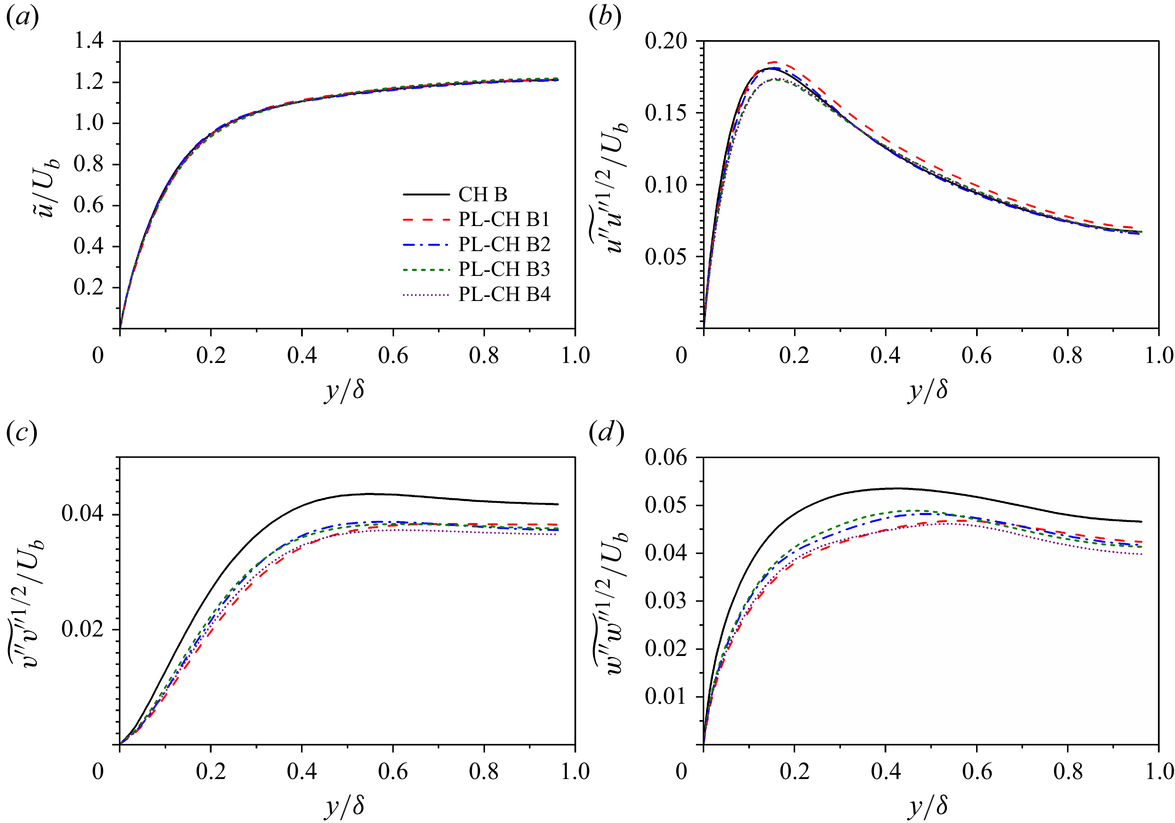
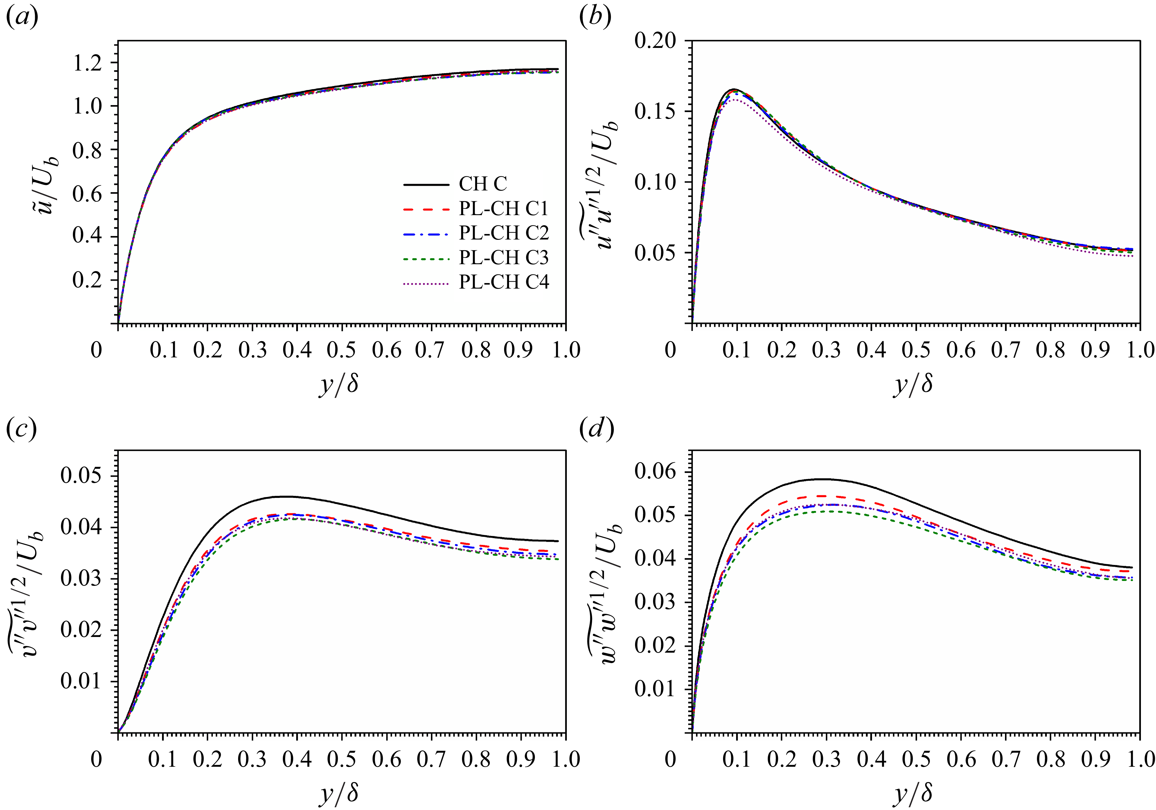
Profiles of (a) density-weighted mean velocity, r.m.s. density-weighted fluctuating velocities normalized by bulk velocity
 $U_b$
in (b) streamwise, (c) wall-normal and (d) spanwise directions for both clean and particle-laden CTCFs at
 ${\textit{Re}}=3000$
and
 ${\textit{Ma}}=3.0$
.
4.1. Fluid velocity
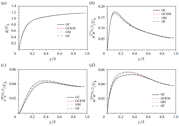
It is shown in figures 11(a), 12(a) and 13(a) that the density-weighted mean streamwise velocities
 $\widetilde {u}$
are not altered by inertial particles in CTCFs, which is consistent with the observations in their incompressible counterparts laden with small particles (Kulick et al. Reference Kulick, Fessler and Eation1994; Vreman Reference Vreman2015). By contrast, it could be very different for the incompressible turbulent channel flows laden with large particles, where the mean streamwise velocity of the fluid phase tends to be attenuated in the near-wall region and enhanced in the outer layer (Uhlmann Reference Uhlmann2008; Shao, Wu & Yu Reference Shao, Wu and Yu2012). Therefore, the large particles may also cause modulation of mean streamwise velocity of fluids in CTCFs. As for turbulence intensity, the r.m.s values of both wall-normal (see figures 11
c, 12
c and 13
c) and spanwise (see figures 11
d, 12
d and 13
d) fluid velocity fluctuations are attenuated by the inertial particles, which is again consistent with their incompressible counterparts laden with small particles (Zhao, Andersson & Gillissen Reference Zhao, Andersson and Gillissen2013; Lee & Lee Reference Lee and Lee2015). However, the finite-sized particles tend to enhance near-wall, wall-normal and spanwise fluctuations of fluid velocities (Shao et al. Reference Shao, Wu and Yu2012) in incompressible turbulent channel flows. Nevertheless, the modulation of streamwise turbulence intensity is complicated and shows no general tendency. In cases with carrier flow CH A, the streamwise fluctuations are attenuated in the very near-wall region, but enhanced in the outer layer. In cases with carrier flow CH B, the streamwise fluctuations are also attenuated in the very near-wall region. However, different behaviours are observed for various
 $St$
numbers in the outer layer. The particles of
 $St=1$
strongly enhance the streamwise turbulent fluctuations along the whole outer layer, while the particles of
 $St$
larger than
 $2$
only slightly enhance the streamwise turbulent fluctuations. Meanwhile, the profiles of streamwise turbulent fluctuations with these Stokes numbers almost collapses onto that in single-phase CTCF at the ending edge of the logarithmic region. In cases with carrier flow CH C, the streamwise fluctuations are attenuated in the near-wall region, and are enhanced in the outer layer for the particles of Stokes number ranging from
 $1$
to
 $3$
. As for particles of
 $St=5$
, the streamwise turbulence intensity is suppressed all along the channel. It can be deduced that the turbulence modulation in CTCFs caused by small particles shares many similarities with respect to their incompressible counterparts. A natural question to be asked is whether the turbulence modulation in CTCFs caused by large finite-sized particles also exhibits similar trends as their incompressible counterparts, which is expected to be studied with particle-resolved simulations in the near future.
Profiles of (a) density-weighted mean velocity, r.m.s. density-weighted fluctuating velocities normalized by bulk velocity
 $U_b$
in (b) streamwise, (c) wall-normal and (d) spanwise directions for both clean and particle-laden CTCFs at
 ${\textit{Re}}=4880$
and
 ${\textit{Ma}}=3.0$
.
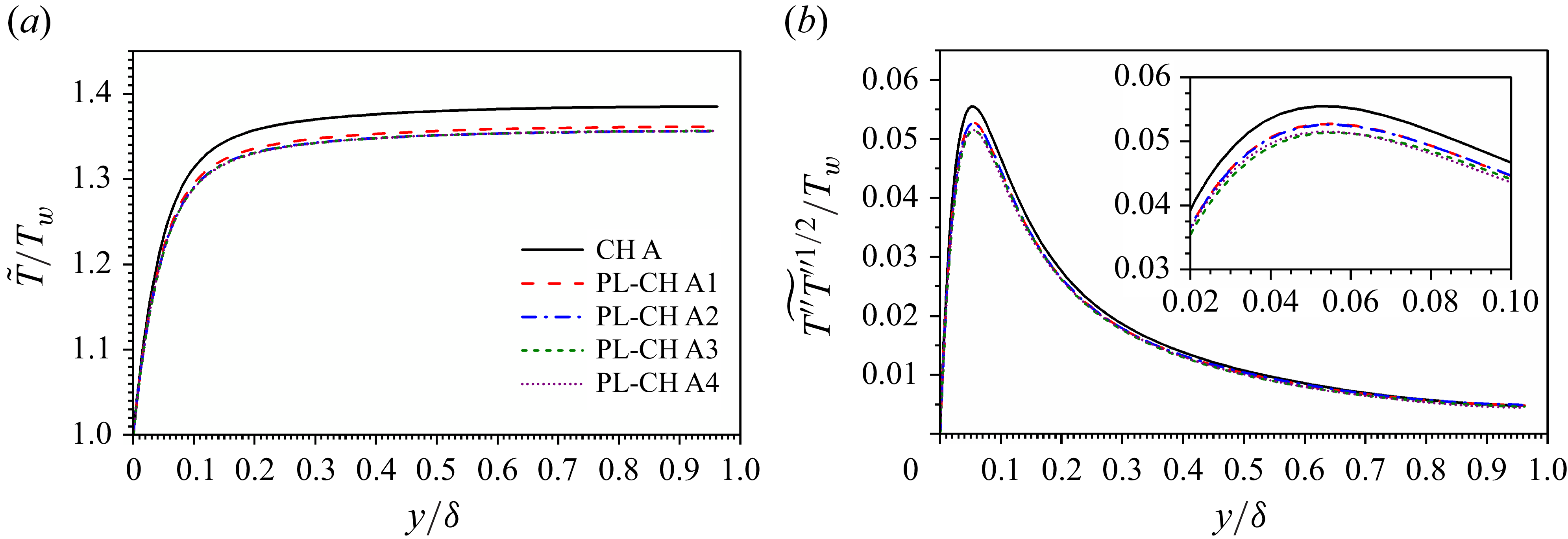
Profiles of (a) density-weighted mean temperature and (b) r.m.s density-weighted fluctuating temperature normalized by wall temperature
 $T_w$
for both clean and particle-laden CTCFs at
 ${\textit{Re}}=3000$
and
 ${\textit{Ma}}=1.5$
.
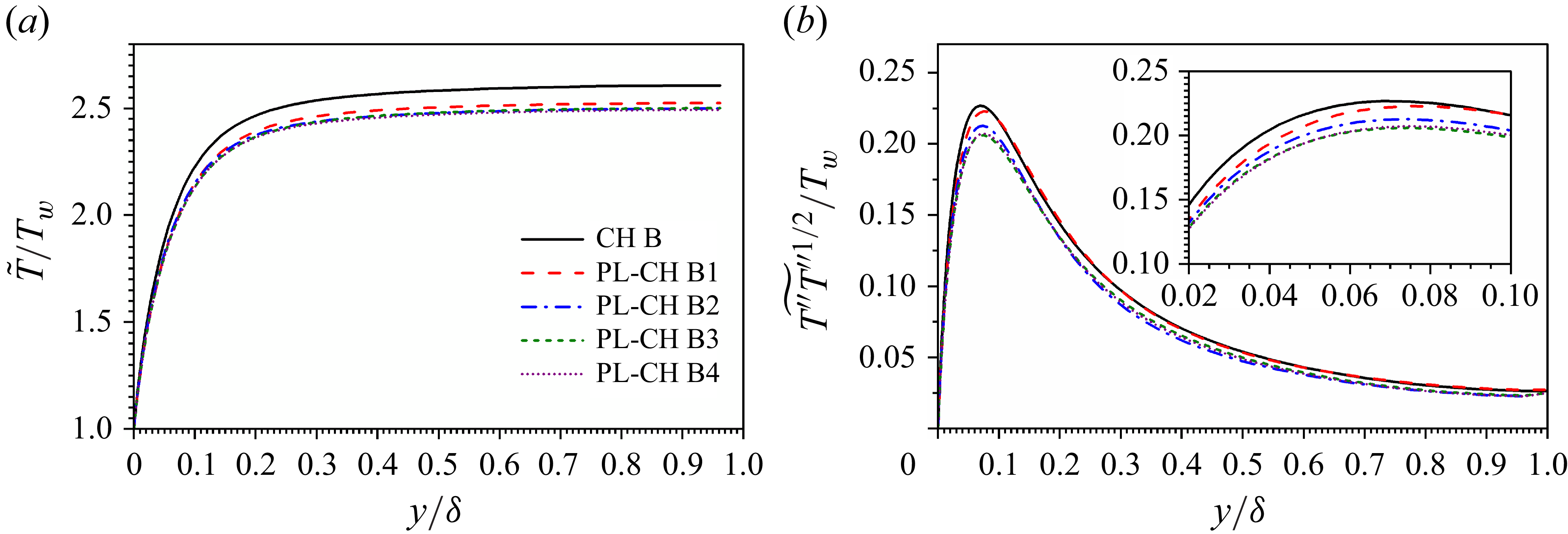
Profiles of (a) density-weighted mean temperature and (b) r.m.s density-weighted fluctuating temperature normalized by wall temperature
 $T_w$
for both clean and particle-laden CTCFs at
 ${\textit{Re}}=3000$
and
 ${\textit{Ma}}=3.0$
.
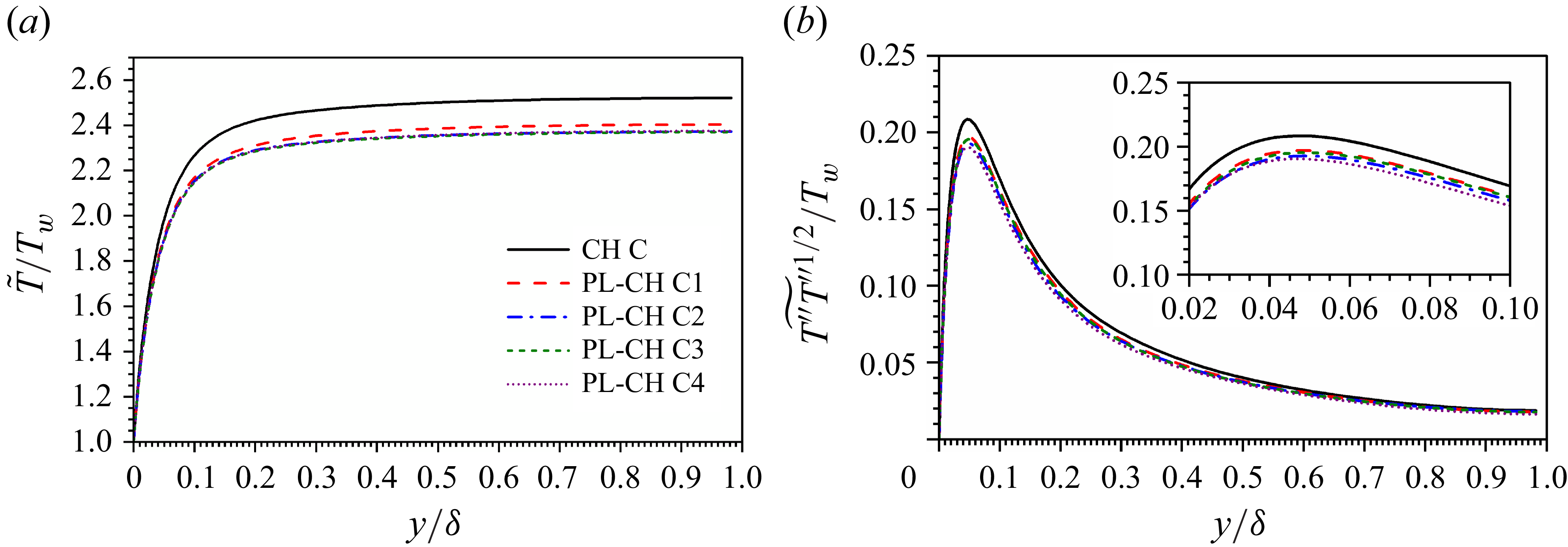
Profiles of (a) density-weighted mean temperature and (b) r.m.s density-weighted fluctuating temperature normalized by wall temperature
 $T_w$
for both clean and particle-laden CTCFs at
 ${\textit{Re}}=4880$
and
 ${\textit{Ma}}=3.0$
.
4.2. Fluid temperature
Unlike the density-weighted mean fluid streamwise velocity, the mean temperature profile
 $\widetilde {T}$
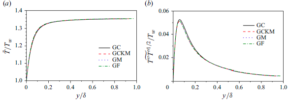
along the wall-normal direction is attenuated by inertial particles in all cases with different carrier flows (see, e.g. figure 14
a for CH A, figure 15
a for CH B and figure 16
a for CH C). However, a similar phenomenon has not been reported either in incompressible turbulent channel flow or in approximately incompressible turbulent channel flow (e.g.
 ${\textit{Ma}} = 0.2$
). This is a very interesting phenomenon because there is no heat transfer between particles and fluids, which implies the kinetic energy transfer between carrier and dispersed phases can eventually cause internal energy modification of carrier phase in CTCFs. Besides, it is usually believed that the small particles alter only the turbulent fluctuations in incompressible turbulent channel flow. However, the evidence exhibited in figures 14(a), 15(a) and 16(a) indicate that the small particles will modulate the mean temperature of background flows. Apart from mean fluid temperature, the temperature fluctuations are also attenuated by small particles as shown in figures 14(b), 15(b) and 16(b). In CTCFs at
 ${\textit{Re}}=3000$
and
 ${\textit{Ma}}=1.5$
, the attenuation of temperature fluctuations occurs mainly in the buffer region. The attenuation of fluctuating temperature can also be found in logarithmic and wake regions with the increase of Reynolds and Mach numbers.
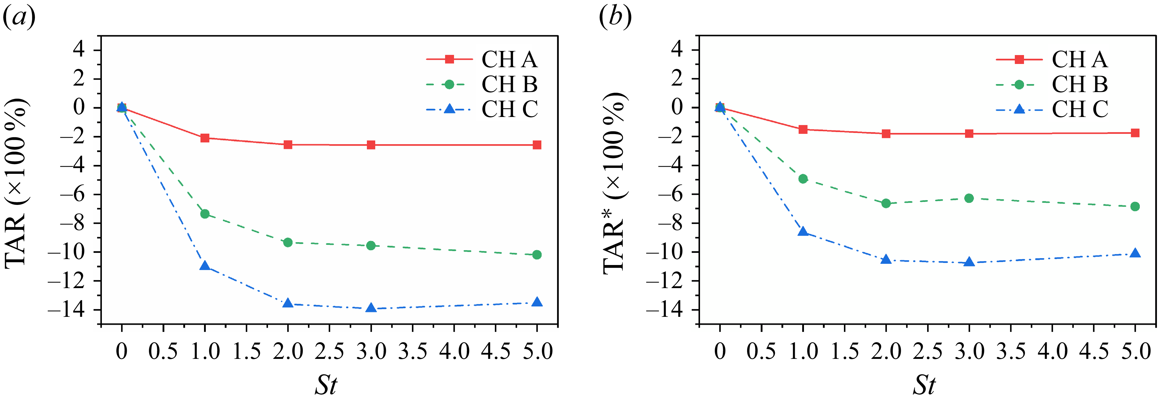
The TARs (a)
 $\mbox{TAR}$
and (b)
 $\mbox{TAR}^*$
with respect to particle Stokes number
 $St$
in particle-laden CTCFs. Three carrier flows are marked by CH A, CH B and CH C, respectively.
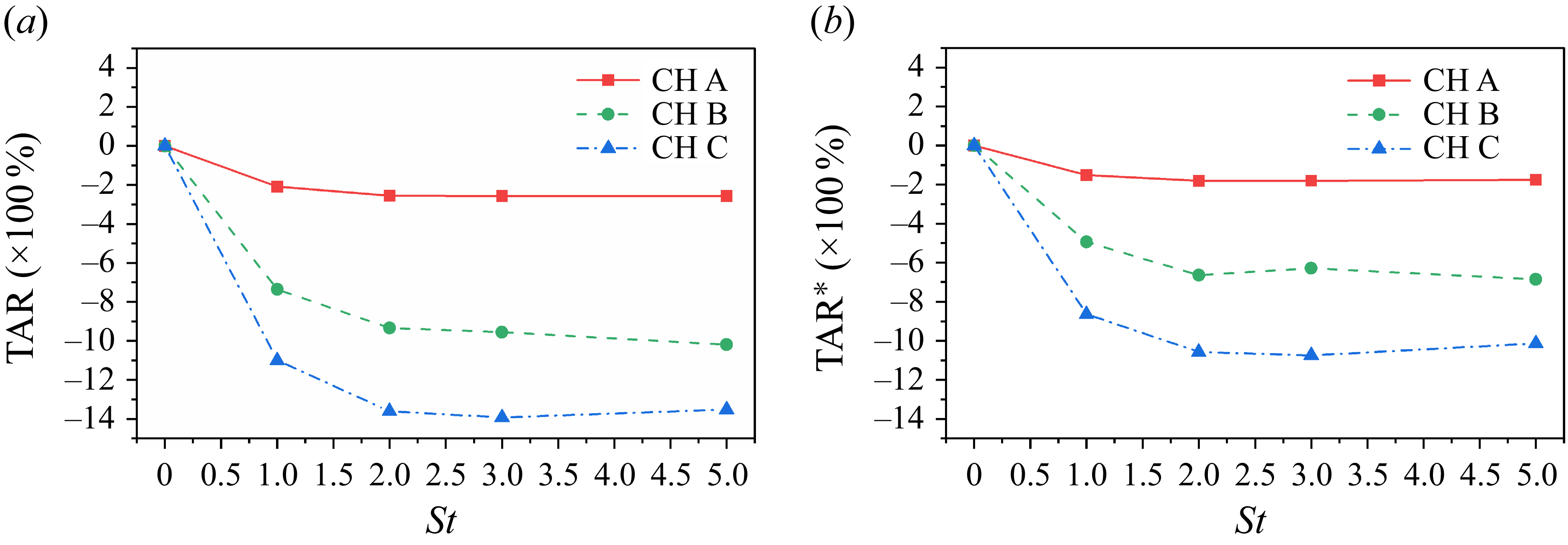
To better characterize the attenuation of mean temperature, a temperature attenuation rate (TAR) is defined as
 \begin{equation} \mbox{TAR} = \frac{1}{T_w \delta } \int _{0}^{\delta } \left(\widetilde {T}_{\textit{PL}}-\widetilde {T}_{\textit{CH}} \right) {\textrm{d}}y, \end{equation}
with
 $\widetilde {T}_{\textit{PL}}$
being the mean temperature profile of particle-laden cases and
 $\widetilde {T}_{\textit{CH}}$
the same profile of clean channel flow cases. A second definition of TAR can be given owing to the independence of mean velocity profiles on particle Stokes number. The equivalent TAR is
 \begin{equation} \mbox{TAR}^* = \frac{1}{T_w u_c}\int _{0}^{u_c} \left(\widetilde {T}_{\textit{PL}}-\widetilde {T}_{\textit{CH}}\right) {\textrm{d}}\widetilde {u}, \end{equation}
with
 $u_c$
being the density-weighted mean velocity at the central plane. Depicted in figures 17(a) and 17(b) are
 $\mbox{TAR}$
and
 $\mbox{TAR}^*$
, respectively, computed using the PP-DNS data. It can be seen from both figures that the overall temperature diminution is strengthened by the increase of Reynolds and Mach numbers, or equivalently the friction Reynolds number. Meanwhile, the temperature attenuation caused by inertial particles is also dependent on the Stokes number. From tracers to inertial particles, the temperature attenuation first increases with particle Stokes number until it reaches a maximum. Then, only slight variation of temperature attenuation is observed with the increase of particle Stokes number. The
 $\mbox{TAR}$
is approximately
 $14\,\%$
compared with the single-phase CTCF in case PL-CH C3, which is a considerable reduction in internal energy of fluid. The value of
 $\mbox{TAR}^*$
is smaller than
 $\mbox{TAR}$
, but presents the same trend, which demonstrates their equivalence. The temperature is treated as a function of velocity in (4.2), which is the key idea of the Reynolds analogy. Therefore, the extension of the Reynolds analogy to multiphase CTCFs is helpful in quantifying the TAR.
4.3. Prediction of TAR
The temperature–velocity relation proposed in this paper (3.29) is used to predict the TAR defined in (4.2), which can be reformulated to
 \begin{equation} \mbox{TAR}^* = \frac{1}{T^*_{w,\textit{PL}}} \int _0^1 T_{\textit{PL}}^* {\textrm{d}} u^* - \frac{1}{T^*_{w,\textit{CH}}} \int _0^1 T_{\textit{CH}}^* {\textrm{d}} u^*. \end{equation}
By using the temperature–velocity relation provided in (3.29), the integral of
 $T^*$
with respect to
 $u^*$
can be obtained as
 \begin{equation} \int _0^1 T^* {\textrm{d}} u^* = T_w^* + \left (\frac{\textit{sPr}}{2} + \frac{1-{\textit{sPr}}}{\beta +2} \right ) \left (T_{rc}^* - T_w^*\right ) + \frac{1}{3} \left (T_c^*-T_{rc}^* \right )\!. \end{equation}
Let
 $c_s$
denote the coefficient
 $sPr/2 + (1-{\textit{sPr}})/(\beta +2)$
, and then
 \begin{equation} \begin{aligned} \frac{1}{T_w^*} \int _0^1 T^* {\textrm{d}} u^* &= 1 + c_s \left ( \frac{T_{rc}}{T_w} - 1 \right ) + \frac{1}{3} \left (\frac{T_{c}}{T_w}-\frac{T_{rc}}{T_w} \right ) \\ &= 1 - c_s + c_s \frac{T_{c}}{T_w} + \left (c_s - \frac{1}{3}\right )\frac{r u_c^2/(2C_{\!p})}{T_w}. \end{aligned} \end{equation}
By substituting (4.5) into (4.3), the TAR,
 $\mbox{TAR}^*$
, can be predicted by present model. According to (4.5), the temperature attenuation caused by inertial particles is attributed to the modulation of Reynolds analogy factor
 $s$
, recovery factor
 $r$
, power exponent in correction function
 $\beta$
and the density-weighted mean temperature and velocity at the central plane
 $T_c$
and
 $u_c$
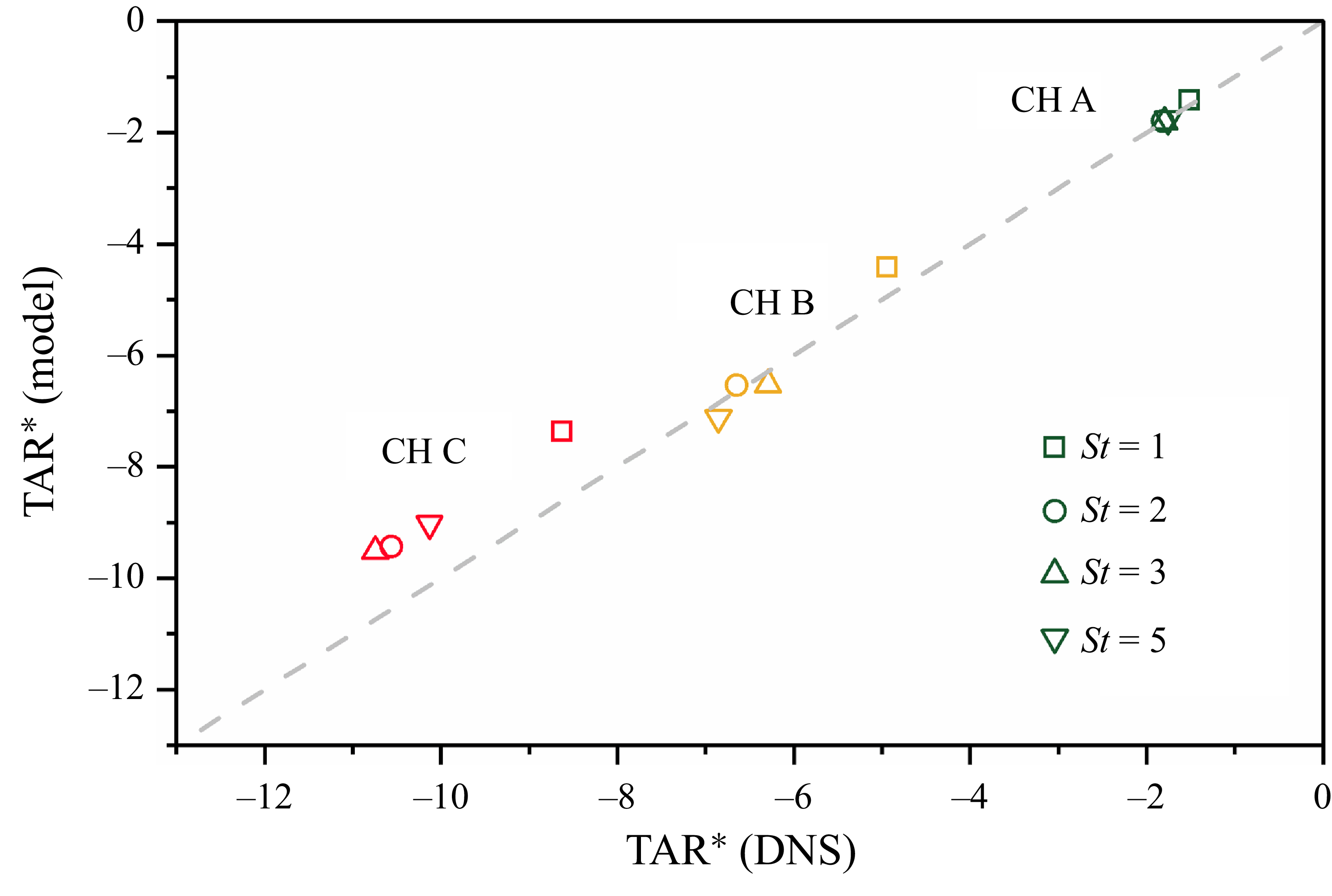
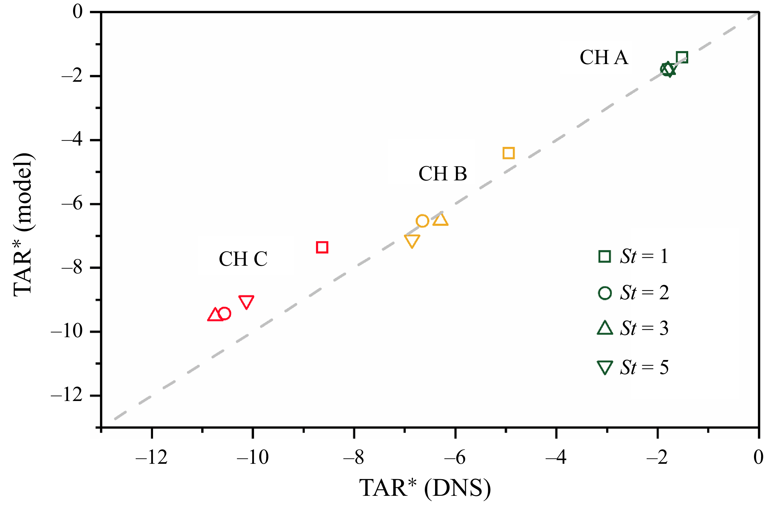
. The results shown in figure 18 manifest that the TAR predicted by the current model agrees well with the DNS data. It should be pointed out, however, that the present model is indeed an a posteriori model. It requires more effort to develop an a priori model to predict TAR.
The TAR,
 $\mbox{TAR}^*$
, obtained from DNS data versus that predicted by present model (4.3). Three carrier flows are marked by CH A, CH B and CH C, respectively, while particles of various inertias are denoted by different symbols.
5. Interphase energy transfer
In § 4.2, the mean temperature of background flow is found to be modulated by inertial particles. The refined Reynolds analogy is successfully applied to predict the TAR. However, the physical mechanism for this temperature attenuation caused by adiabatic particles still remains unclear. In this section, the origin of such an internal energy loss is explored with the help of an analysis of energy exchange in the particle-laden CTCFs.
Pathways for energy transfer between dispersed phase and carrier phase in CTCFs. The solid arrows represent one-way energy transfer and the dashed arrows represent two-way energy transfer. The definitions of the symbol are listed as follows:
 $Q_i \equiv \overline {\rho } \widetilde {f_i} \widetilde {u_i}$
is the energy injected into the mean flow via external body force;
 $\varLambda ^m \equiv \overline {\rho }\widetilde {\varphi _i} \widetilde {u_i}$
is the kinetic energy exchange between particles and mean flow;
 $\varLambda ^t \equiv \overline {\rho } \widetilde {\varphi ^{\prime \prime}_i u^{\prime \prime}_i}$
is the kinetic energy exchange between particles and turbulence;
 $P_k \equiv -\overline {\rho } \widetilde {u^{\prime \prime}_i u^{\prime \prime}_{\!j}} \partial \widetilde {u_i} / \partial x_{\!j}$
is the turbulence production;
 $\phi ^{Mp} \equiv \overline {u^{\prime \prime}_i}\partial \overline {p}/\partial x_i$
is the pressure work;
 $\phi ^{M\nu } \equiv -\overline {u^{\prime \prime}_i}\partial \overline {\sigma _{ij}}/\partial x_{\!j}$
is the viscous work;
 $\mathcal{E} \equiv \overline {\sigma _{ij}} \partial \overline {u_i}/\partial x_{\!j}$
is the mean dissipation;
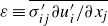 $\varepsilon \equiv \overline {\sigma ^{\prime}_{ij} \partial u^{\prime}_i/\partial x_{\!j}}$
is the turbulent dissipation;
 $\varPi ^m \equiv \overline {p} \partial \overline {u_i}/\partial x_i$
is the mean pressure dilatation;
 $\varPi ^p \equiv \overline {p^{\prime} \partial u^{\prime}_i /\partial x_i}$
is the pressure-strain term.
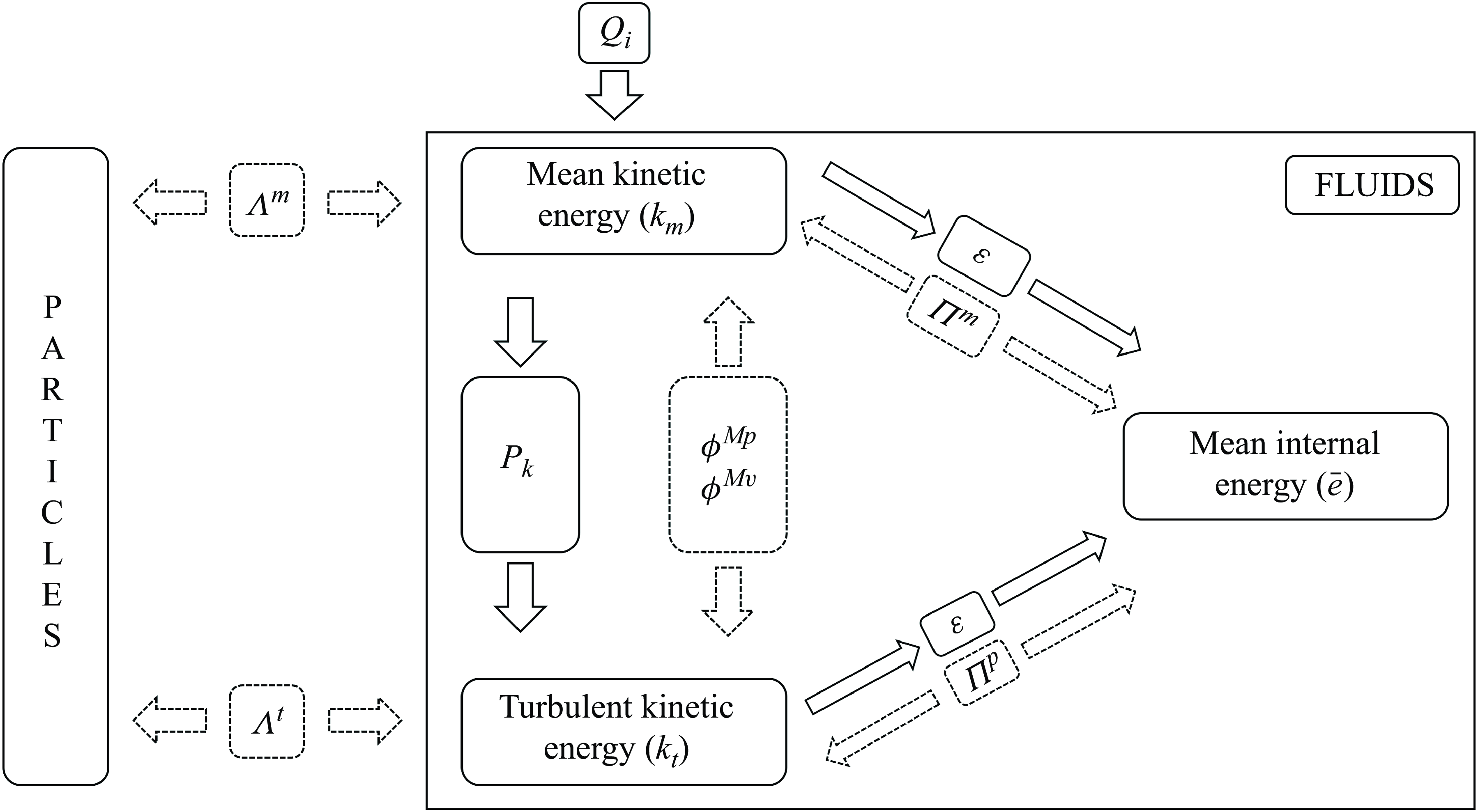
In general, the total energy of fluid consists of two parts, i.e. the kinetic energy
 $k \equiv \rho u_i u_i/2$
and internal energy
 $e \equiv \rho C_V T$
. The Reynolds-averaged kinetic energy
 $\overline {k}$
can be further divided into the kinetic energy of mean flow
 $k_m \equiv \overline {\rho } \widetilde {u}_i \widetilde {u}_i/2$
and the turbulent kinetic energy
 $k_t = \overline {\rho } \widetilde {u_i^{\prime \prime}u_i^{\prime \prime}}/2$
. Similarly, the internal energy can also be split into a mean part and a fluctuating part by introducing a diagnostic variable (Mittal & Girimaji Reference Mittal and Girimaji2019; Fan et al. Reference Fan, Li and Pirozzoli2022). In this study, focus is placed on the mean temperature, i.e. mean internal energy. Thus, it is sufficient to consider the Reynolds-averaged internal energy
 $\overline {e}$
, which is the internal energy of the mean flow. The objective of this section is to analyse the energy transfer among
 $k_m$
,
 $k_t$
and
 $\overline {e}$
. The detailed derivations for the governing equations of
 $k_m$
,
 $k_t$
and
 $\overline {e}$
are given in Appendix B. Here, we show directly in figure 19 the pathway for energy transfer between dispersed phase and carrier phase. The definition of each term in figure 19 is also provided in Appendix B.
Premultiplied profiles of (a) turbulent kinetic production, (b) mean viscous dissipation, (c) turbulent viscous dissipation and (d) mean particle feedback in both single-phase and particle-laden CTCFs at
 ${\textit{Re}}=3000$
and
 ${\textit{Ma}} = 1.5$
. All quantities are normalized by the corresponding wall units of the single-phase CTCF.
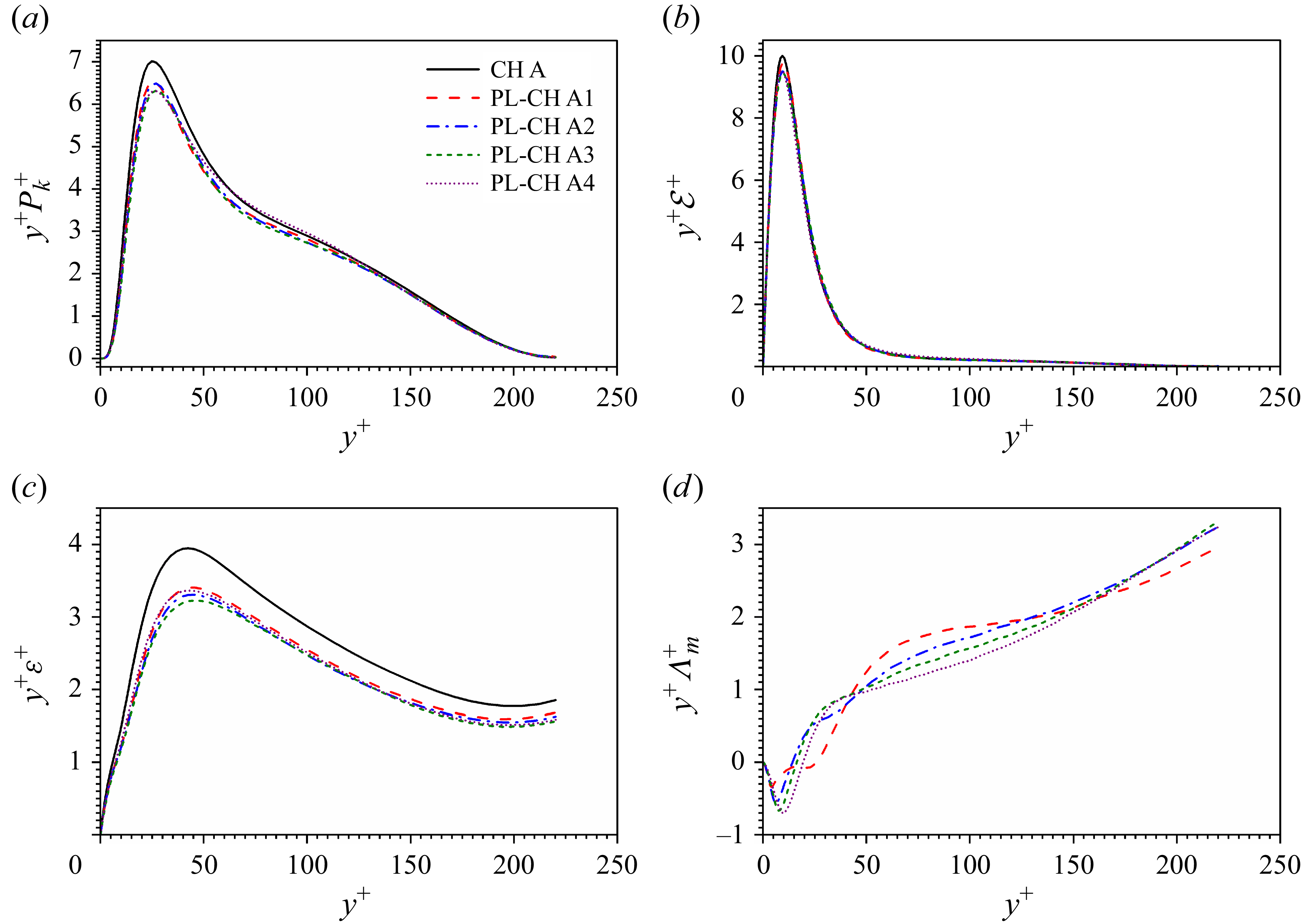
Premultiplied profiles of (a) turbulent kinetic production, (b) mean viscous dissipation, (c) turbulent viscous dissipation and (d) mean particle feedback in both single-phase and particle-laden CTCFs at
 ${\textit{Re}}=3000$
and
 ${\textit{Ma}} = 3$
. All quantities are normalized by the corresponding wall units of the single-phase CTCF.
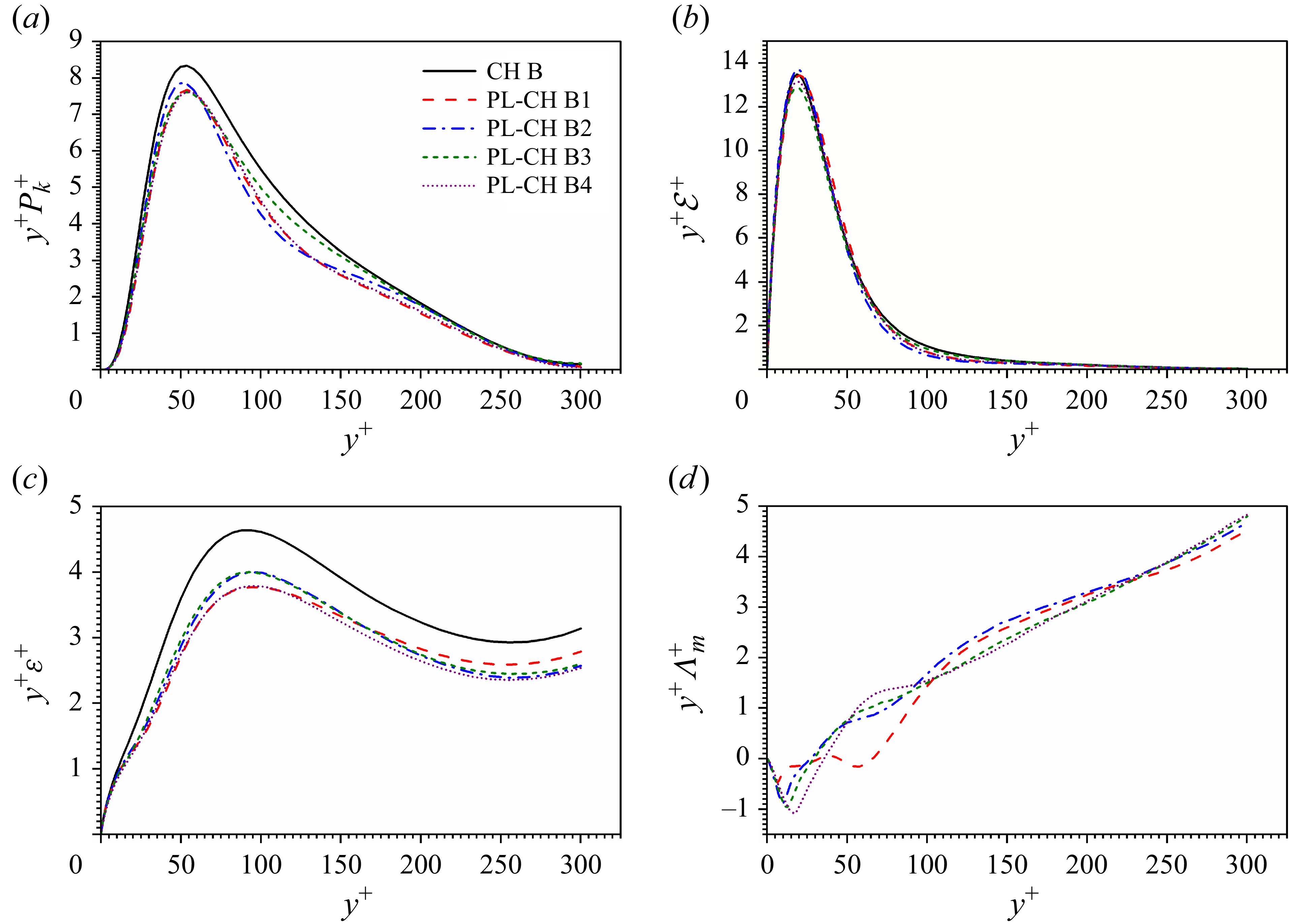
Premultiplied profiles of (a) turbulent kinetic production, (b) mean viscous dissipation, (c) turbulent viscous dissipation and (d) mean particle feedback in both single-phase and particle-laden CTCFs at
 ${\textit{Re}}=4880$
and
 ${\textit{Ma}} = 3$
. All quantities are normalized by the corresponding wall units of the single-phase CTCF.
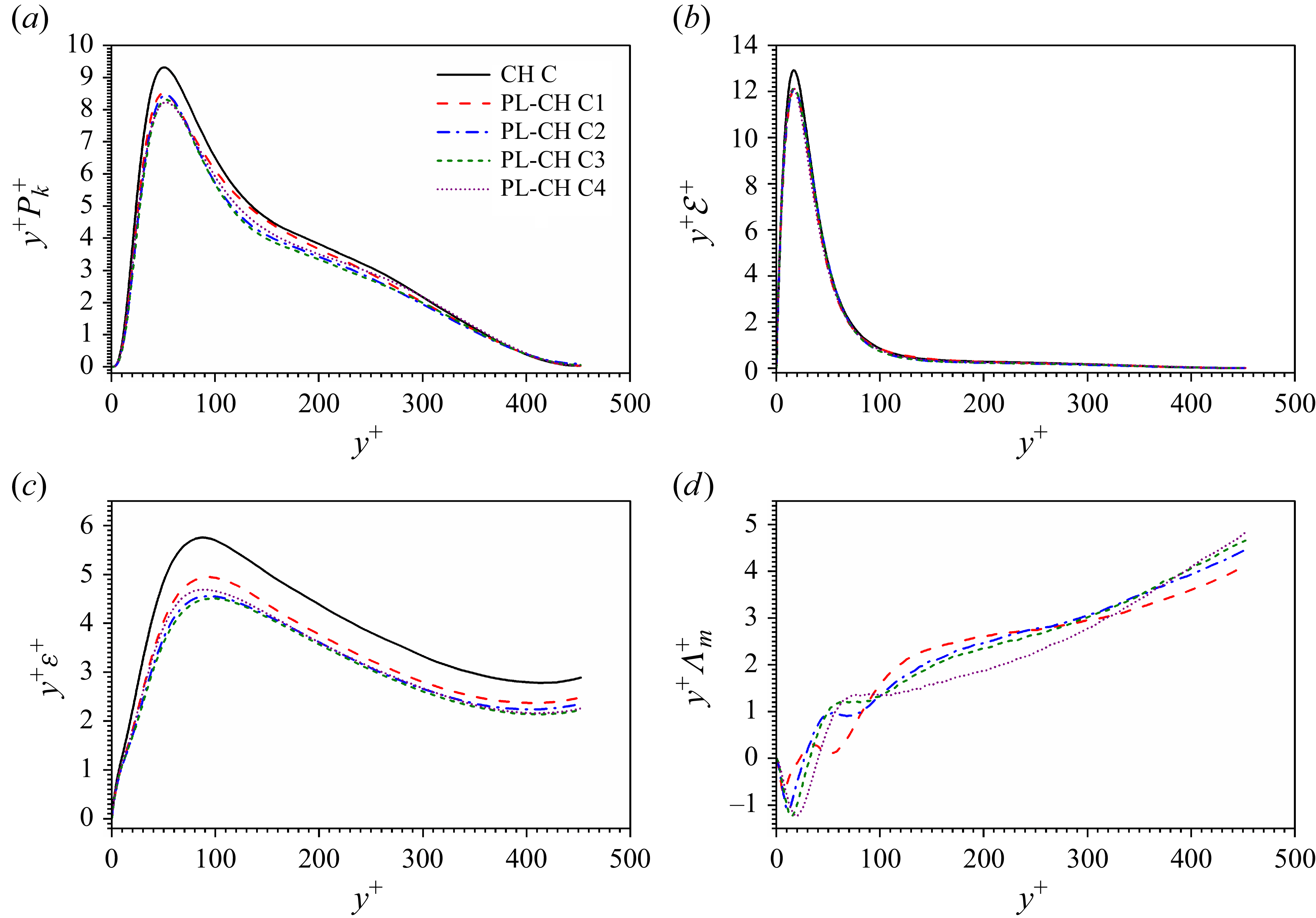
The pathway for energy transfer between dispersed phase and carrier phase is sketched in figure 19. The external body force first injects kinetic energy into the mean flow via
 $Q_i$
to maintain a constant mass flux. Then, the dispersed phase exchanges kinetic energy with the mean flow by
 $\varLambda ^m$
and the turbulence by
 $\varLambda ^t$
. There are three main pathways of energy transfer within the carrier phase, including
 $k_m$
–
 $k_t$
exchange dominated by turbulent production
 $P_k$
,
 $k_m$
–
 $\overline {e}$
exchange dominated by mean viscous dissipation
 ${\mathcal{E}}$
, and
 $k_t$
–
 $\overline {e}$
exchange dominated by turbulent viscous dissipation
 $\varepsilon$
.
In single-phase CTCFs, the injected energy
 $Q_i$
is balanced with mean viscous dissipation and turbulent production, which is indicated by the balance law of total shear stress. However, this balance law no longer holds for particle-laden CTCFs because the mean flow exchanges energy with the dispersed phase via
 $\varLambda ^m$
. As shown in figures 20–22(d),
 $\varLambda ^m$
is positive along the wall-normal direction except for the very near-wall region, which indicates that the carrier phase gives kinetic energy to the dispersed phase. As a result, the turbulent production
 $P_k$
and mean viscous dissipation in particle-laden CTCFs must be smaller than in single-phase CTCFs. These observations are confirmed by the numerical results shown in figures 20–22(a) and 20–22(b). On the one hand, the modulation of
 ${\mathcal{E}}$
by inertial particles is weak and can only be observed in a very small region of buffer layer at
 $y^+ \approx 25$
. Apart from this region, there exhibits almost no modulation of
 ${\mathcal{E}}$
in the channel. Therefore, it is assumed in this study that the modulation of
 $E$
is negligible. On the other hand, the attenuation of turbulent production
 $P_k$
caused by particles is much more significant compared with
 ${\mathcal{E}}$
. It can not only be observed in the near-wall regions, but also in the logarithmic regions. Therefore, the attenuation of turbulent production is considered as the major consequence of energy exchange between dispersed phase and mean flow.
The attenuation of turbulent production
 $P_k$
results directly in the reduction of turbulence dissipation
 $\varepsilon$
. Similar trends have been observed in CTCFs at low Mach numbers (Ruan & Xiao Reference Ruan and Xiao2024b
), which can be interpreted by the balance law between the turbulent production and dissipation. Significant attenuation of turbulent dissipation is observed in all cases considered in the current study as shown in figures 20–22(c). The diminution of
 $\varepsilon$
is important all along the wall-normal direction, even at the central plane of the channel. Previous numerical simulations reveal that large particles of high Stokes number will enhance turbulence dissipation in both incompressible homogeneous isotropic turbulence (Shao et al. Reference Shao, Wu and Yu2012) and incompressible turbulent channel flows (Yu et al. Reference Yu, Xia, Guo and Lin2021). However, both numerical simulation (Lee & Lee Reference Lee and Lee2015) and experimental measurement (Paris Reference Paris2001) report that small particles of high Stokes number will attenuate turbulence dissipation, which supports the conclusion drawn from present numerical simulations. Thus, it can be deduced that the modulation of turbulence dissipation caused by particles is influenced not only by particle inertia but also by particle diameter. For the small PPs considered in this paper, the turbulence dissipation is indeed attenuated by the particles. The mean flow dissipation
 ${\mathcal{E}}$
and the turbulent dissipation
 $\varepsilon$
are the two major sources for the mean internal energy
 $\overline {e}$
. The former is hardly altered by the inertial particles in CTCFs. Therefore, the attenuation of the latter sheds light on the origin of a lower mean temperature in particle-laden CTCFs compared with the single-phase case. Meanwhile, for CTCFs laden with large particles, the mean temperature might be enhanced due to the augmentation of turbulence dissipation caused by large particles according to the energy pathway. Besides, large particles also tend to modulate the mean velocity of fluids, i.e. the mean flow dissipation, whose influence on temperature modulation must be taken into account. The emergence of particle-resolved numerical simulations can be of great help to investigate the temperature modulation caused by large particles. Last but not least, particles (especially large particles) are often considered as a good carrier for thermal mixing. Hence, the heat transfer is conjectured to be another important factor for the temperature modulation in CTCFs, which is left as an open and interesting question for further research.
According to the energy pathway analysis, the temperature attenuation caused by small particles is attributed to the attenuation of turbulence dissipation. Therefore, the effect of particle mass fraction on temperature attenuation can be assessed indirectly by evaluating the change of turbulence dissipation. In outer layer of CTCFs, the turbulence dissipation is approximately balanced by turbulence production. Meanwhile, the turbulence production term is a function of the Reynolds stress. According to the stress balance, the Reynolds stress is dependent on the particle feedback force by
 \begin{equation} -\overline {\rho } \widetilde {\ u^{\prime \prime}v^{\prime \prime}} + \int _{0}^{y} \overline {\rho \varphi _2} {\textrm{d}} y + \overline {\mu } \frac{{\textrm{d}} \widetilde {u}}{{\textrm{d}} y} = \tau (y). \end{equation}
As the mean shear almost remains unchanged in the presence of small particles, the sum of Reynolds stress and particle feedback force is approximately constant in CTCFs. Thus, the variation of turbulence dissipation can be evaluated by the change of Reynolds stress
 \begin{equation} \Delta \varepsilon \approx \int _{0}^{y} \overline {\rho \varphi _2} {\textrm{d}} y \frac{{\textrm{d}} \widetilde {u}}{{\textrm{d}} y}, \end{equation}
which is responsible for the turbulence production. The particle feedback force is approximately equivalent to
 \begin{equation} \overline {\rho \varphi _2} \approx \overline { \frac{n_{\!p} \rho _{\!p} \pi d^3/6}{\rho \Delta\!V} \rho a_{p,2}} \approx \overline {\rho \psi a_{p,2}}, \end{equation}
with
 $\psi$
being the local particle mass fraction in a fluid cell and
 $a_{p,2}$
being the particle acceleration in the wall-normal direction. As a result, the attenuation of turbulent dissipation is proportional to the particle mass fraction. Therefore, the temperature attenuation is expected to be proportional to the particle mass fraction according to the energy pathway. Besides, (5.2) and (5.3) suggest that the attenuation of turbulent dissipation is dependent on the particle acceleration in the wall-normal direction
 $a_{p,2}$
, which can help interpret the saturation of
 $\mbox{TAR}$
and
 $\mbox{TAR}^*$
as observed in figure 17. Phenomenologically, particles become more ballistic with the increase of Stokes number, and the particle motions are less sensitive to the background turbulence accordingly. Theoretically, the particle acceleration
 $a_{p,2}$
is affected by both Stokes drag
 $a_{p,2}^{D}$
and Saffman lift
 $a_{p,2}^{L}$
according to (2.8), which can be evaluated by
 \begin{equation} a_{p,2}^{D} \sim \frac{v - v_{\!p}}{\tau _{\!p}} \end{equation}
and
 \begin{equation} a_{p,2}^{L} \sim d \frac{u - u_{\!p}}{\tau _{\!p}}, \end{equation}
respectively, with
 $u$
and
 $u_{\!p}$
being the fluid and particle velocities in streamwise direction,
 $v$
and
 $v_{\!p}$
the fluid and particle velocities in wall-normal direction,
 $\tau _{\!p}$
the particle relaxation time and
 $d$
the particle diameter. Here,
 $v$
is essentially fluctuating velocity component in the wall-normal direction since the wall-normal mean velocity is zero. Therefore, the particle motion in the wall-normal direction is dominated by the turbulent fluctuations. For the particles of large Stokes numbers under consideration, the particle relaxation time
 $\tau _{\!p}$
is larger than the Kolmogorov time scale
 $\tau _k$
but smaller than the integral time
 $\tau _L$
(the characteristic time scale corresponding to the integral length scale
 $L$
) due to the constraint of PP hypothesis. The equilibrium Eulerian approximation (Balachandar Reference Balachandar2009) suggests that the slip velocity
 $v-v_{\!p}$
for the particles with
 $\tau _k\lt \tau _{\!p}\lt \tau _L$
obeys the scaling law
 \begin{equation} v-v_{\!p} \sim \left ( \frac{\tau _{\!p}}{\tau _k} \right )^{1/2} u_k, \end{equation}
where
 $u_k$
is a characteristic velocity corresponding to the Kolmogorov scale. With the help of scaling analysis, one can readily obtain
 $a_{p,2}^{D} \sim \tau _{\!p}^{-1/2}$
, which is negligible when
 $\tau _{\!p}$
is sufficient large. By contrast, it requires more effort to handle the particle acceleration caused by lift force owing to the presence of mean background flow in streamwise direction. To this end, the particle acceleration caused by lift force is decomposed into two parts, i.e. a mean part and a fluctuating part, in the form
 \begin{equation} a_{p,2}^{L} \sim d \frac{\overline {u}-\overline {u}_{\!p}}{\tau _{\!p}} + d \frac{u^{\prime}-u^{\prime}_{\!p}}{\tau _{\!p}}. \end{equation}
Given that
 $\overline {u} - \overline {u}_{\!p}\lt u_c$
and
 $d \sim \tau _{\!p} ^{1/2}$
(Ruan & Xiao Reference Ruan and Xiao2024b
), the mean contribution can be rewritten as
 \begin{equation} d \frac{\overline {u}-\overline {u}_{\!p}}{\tau _{\!p}} \sim u_c \tau _{\!p}^{-1/2}, \end{equation}
where
 $u_c$
is the mean streamwise velocity at the centreplane. As for the fluctuating contribution, the same scaling law as the wall-normal exponent applys, i.e.
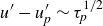 $u^{\prime}-u^{\prime}_{\!p} \sim \tau _{\!p}^{1/2}$
, which leads to
 \begin{equation} d \frac{u^{\prime}-u^{\prime}_{\!p}}{\tau _{\!p}} \sim {O}(1). \end{equation}
Therefore, the mean contribution to
 $a_{p,2}^{L}$
approaches zero with the increase of
 $\tau _{\!p}$
while the fluctuating contribution to
 $a_{p,2}^{L}$
is independent on the particle relaxation time, i.e. the particle Stokes number. As the particle Stokes number becomes larger and larger,
 $a_{p,2}^{D}$
and the mean contribution to
 $a_{p,2}^{L}$
tend to zero while the fluctuating contribution to
 $a_{p,2}^{L}$
remains unchanged. In such situations, the particle acceleration in the wall-normal direction
 $a_{p,2}$
tends to be independent of particle Stokes number, which leads to the saturation of
 $\Delta \varepsilon$
(and as a result, of
 $\mbox{TAR}$
and
 $\mbox{TAR}^*$
) as the mass fraction
 $\psi$
is kept unchanged in present simulations. It needs to be stressed that the lift force plays a significant role for the attenuation of turbulent dissipation in particle-laden turbulent channel flows, which is also consistent with the conclusion of our previous research (Ruan & Xiao Reference Ruan and Xiao2024b
).
6. Conclusions and discussions
In this paper, the Reynolds analogy is established for fully developed particle-laden CTCFs by following the theoretical framework developed by van Driest. It is found that the van Driest approach can be applied to fully developed CTCFs driven by body force under the statistically steady hypothesis in one dimension. The failure of Walz’s equation in predicting the temperature–velocity relation in CTCFs is attributed to the poor quality for estimation of
 $S$
given in (3.19). To this end, a correction function is introduced to improve the prediction accuracy of Walz’s equation, which is supposed to be proportional to
 $1-{u^*}^{\beta }$
. The improved model degenerates to GRA when the correction function takes a linear form. To better agree with numerical observations, the power exponent in correction function is set to
 $1.27$
. The newly proposed model is in very good consistence with the numerical simulation for single-phase CTCFs.
The same methodology is then employed to study the particle-laden CTCFs. It is manifested that the power exponent of the correction function in particle-laden cases is smaller than that in single-phase CTCFs. Numerical data fitting indicates that the power exponent
 $\beta$
follows a scaling law
 $St^{0.08}$
for particle-laden CTCFs. The new model successfully cuts the relative error by half between model prediction and PP-DNS results of temperature–velocity relation compared with GRA. It also needs to be pointed out that the two key parameters in theoretical modelling, the Reynolds analogy factor and recovery factor, are all reduced due to the presence of inertial particles.
Furthermore, the turbulence modulation in fluid velocity and temperature caused by inertial particles is investigated in particle-laden CTCFs based on two-way coupling PP-DNS. The numerical results imply that the mean streamwise velocity of background flow remains unchanged when interacting with inertial particles. However, it should be emphasized that the mean temperature of background flow is attenuated by inertial particles even though there exists no heat transfer between particles and carrier fluids. Besides, the velocity fluctuations in wall-normal and spanwise directions, the streamwise velocity fluctuations below the buffer region and temperature fluctuations are also found to be reduced due to the inertial particles. The attenuation of mean temperature is strengthened with the increase in particle Stokes number and Mach number in the range of interest in present study. Two equivalent TARs are defined to describe the modulation of mean temperature. It is found that the TAR is considerable when the particle Stokes number or Mach number become larger. Moreover, the refined Reynolds analogy is used to predict the
 $\mbox{TAR}^*$
caused by inertial particles, which is defined as the integral of mean temperature normalized by wall temperature with respect to mean velocity normalized by its value at the central plane. The theoretical predictions agree pretty well with the numerical results.
In addition, the energy transfer pathway is established for particle-laden CTCFs to reveal the physical mechanism for the attenuation of temperature caused by inertial particles. In general, the mean flow injects energy to turbulence via the turbulence production term. Because the inertial particles gain kinetic energy from the mean flow, the Reynolds stress (and as a result, the turbulence production) is reduced compared with the single-phase case, leading to the reduction in turbulent kinetic energy. In other words, the mean flow injects less energy into turbulence in the particle-laden case. The attenuation of turbulence production further causes the decrease of turbulent dissipation. It is the suppression of turbulent dissipation that eventually results in the temperature attenuation in particle-laden CTCFs.
It should be stressed that the methodology proposed in this paper can be applied to other types of internal compressible wall-bounded turbulent flows laden with inertial particles, such as compressible turbulent pipe flows. It is also conjectured that the present analysis method can be extended to the compressible turbulent boundary layers with zero pressure gradient. However, it cannot be directly extended to compressible turbulent boundary layers with different types of pressure gradients, which is left as an open question for future research. Besides, the particle-resolved numerical simulations are encouraged to provide an insight into the influence of particle size and particle shape.
Acknowledgement
Numerical simulations were carried out on the Polars computing platform of Peking University in Beijing, China. Special thanks are addressed to X. Li for providing the single-phase fluid solver Opencfd-SC Ver 2.2b. The authors appreciate the kind gesture from G. N. Coleman in providing the DNS data for comparison. The authors would also like to thank H. Qi for providing the large-eddy simulation data to generate an initial flow field for DNS.
Funding
The authors acknowledge the financial supports provided by National Natural Science Foundation of China under grants no. 92152202 and no. 12588201.
Declaration of interests
The authors report no conflict of interest.
Appendix A.
To confirm the validity of the numerical results presented in this paper, a grid-dependence test is conducted for the numerical simulation of compressible channel flow at
 ${\textit{Re}}=3000$
and
 ${\textit{Ma}} = 1.5$
laden with particles of
 $St=3$
, i.e. the case PL-CH A3. The numerical simulations are conducted on four different grids with their resolutions given in table 4. The case GM corresponds to the grid resolution employed in the main text. The case GCKM corresponds to a grid resolution used in the literature (Coleman et al. Reference Coleman, Kim and Moser1995). The cases GF and GC are two newly designed runs with finer and coarser grid resolutions than case GM.
Grid numbers and grid sizes in different simulations for case PL-CHA3.
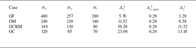
Profiles of (a) mean streamwise velocity, (b) r.m.s. streamwise velocity fluctuations, (c) r.m.s. wall-normal velocity fluctuations and (d) r.m.s. spanwise velocity fluctuations of fluid phase computed on different grids.
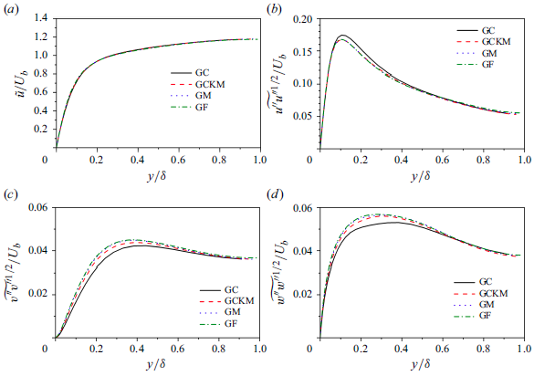
Profiles of (a) mean temperature and (b) r.m.s. temperature fluctuations of fluid phase computed on different grids.
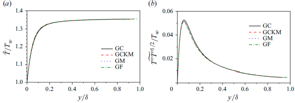
Shown in figures 23(a) and 24(a) are mean streamwise velocity and temperature profiles, respectively, obtained on different grids. It is observed that the numerical results under different grids collapse with each other, which indicates that the mean streamwise velocity and temperature are relatively not sensitive to the grid resolutions under consideration. The turbulence statistics including turbulent intensities in the streamwise, wall-normal and spanwise directions as well as temperature fluctuations are further examined to study the grid-dependence property. Figures 23(a–c) and 24(b) suggest that the velocity and temperature fluctuations are indeed dependent on the grid resolutions. Coarse grids tend to overestimate the streamwise turbulent intensity and temperature fluctuations, while the wall-normal and spanwise turbulent intensities are underestimated on coarse grids. However, the velocity and temperature fluctuations show a converging tendency when increasing the grid resolutions. The turbulent intensities and temperature fluctuations on grids GM and GF almost collapse onto each other, which indicates that the numerical simulations on grid GM are reliable.
Appendix B.
B.1. Kinetic energy
To study the energy transfer between
 $k_m$
and
 $k_t$
, one needs to obtain the governing equations of
 $k_m$
and
 $k_t$
. The equation of
 $k_m$
can be obtained from the averaged momentum equation. However, the equation of
 $k_t$
can only be obtained by subtracting the equation of
 $k_m$
from the equation of
 $\overline {k}$
. Therefore, we begin with the derivation of the equation for averaged kinetic energy.
By multiplying both sides of (2.2) by
 $u_i$
and subtracting
 $u_i u_i /2$
times both sides of (2.1), one obtains the equation of total kinetic energy as
 \begin{equation} \frac{\partial k}{\partial t} + \frac{\partial k u_{\!j}}{\partial x_{\!j}} = - \frac{\partial p u_i}{\partial x_i} + p\frac{\partial u_i}{\partial x_i} + \frac{\partial \sigma _{\textit{ij}} u_i }{\partial x_{\!j}} - \sigma _{\textit{ij}} \frac{\partial u_i}{\partial x_{\!j}} +\rho f_i u_i- \rho \varphi _i u_i. \end{equation}
The Reynolds average of (B1) introduces
 $\overline {ku_{\!j}}$
, which reads
 \begin{equation} \overline {ku_{\!j}} = k_m \widetilde {u}_{\!j} + k_t \widetilde {u}_{\!j} + \overline {\rho } \widetilde {u^{\prime \prime}_i u^{\prime \prime}_{\!j}} \widetilde {u}_i + \frac{1}{2} \overline {\rho } \widetilde { u^{\prime \prime}_i u^{\prime \prime}_i u^{\prime \prime}_{\!j}}. \end{equation}
Therefore, the averaged equation of kinetic energy is written as
 \begin{align} \frac{ \partial \overline {k}}{\partial t} + \frac{ \partial \overline {k} \widetilde {u}_{\!j} }{\partial x_{\!j}} &= -\frac{\partial \overline {\rho } \widetilde {u^{\prime \prime}_i u^{\prime \prime}_{\!j}} \widetilde {u}_i}{\partial x_{\!j}} - \frac{1}{2} \frac{\partial \overline {\rho } \widetilde { u^{\prime \prime}_i u^{\prime \prime}_i u^{\prime \prime}_{\!j}}}{\partial x_{\!j}} - \frac{\partial \overline {p u_i} }{\partial x_i} + \overline {p \frac{\partial u_i }{\partial x_i} } \nonumber \\ &\quad +\, \frac{\partial \overline {\sigma _{\textit{ij}} u_i} }{\partial x_{\!j}} - \overline {\sigma _{\textit{ij}} \frac{\partial u_i}{\partial x_{\!j}} } + \overline {\rho } \widetilde {f_i u_i} - \overline {\rho } \widetilde {\varphi _i u_i}. \end{align}
To derive the governing equation of
 $k_m$
, Favre-averaging is first applied to (2.2) to obtain
 \begin{equation} \frac{\partial \overline {\rho } \widetilde {u_i} }{\partial t} + \frac{\partial \overline {\rho } \widetilde {u_i} \widetilde {u_{\!j}}}{\partial x_{\!j}} = -\frac{\partial \overline {\rho } \widetilde {u^{\prime \prime}_i u^{\prime \prime}_{\!j}} }{\partial x_{\!j}} -\frac{\partial \overline {p} }{\partial x_i} + \frac{\partial \overline {\sigma _{\textit{ij}}}}{\partial x_{\!j}} + \overline {\rho } \widetilde {f_i} - \overline {\rho } \widetilde {\varphi }_i. \end{equation}
Then, multiplying (B4) by
 $\widetilde {u_i}$
and subtracting
 $\widetilde {u_i} \widetilde {u_i} /2$
times
 $\overline {(2.1)}$
yield the equation of
 $k_m$
in the form
 \begin{align} \frac{\partial k_m}{\partial t} + \frac{\partial k_m \widetilde {u_{\!j}} }{\partial x_{\!j}} & = - \frac{\partial \overline {\rho } \widetilde {u^{\prime \prime}_i u^{\prime \prime}_{\!j}} \widetilde {u_i} }{\partial x_{\!j}} +\overline {\rho } \widetilde {u^{\prime \prime}_i u^{\prime \prime}_{\!j}}\frac{\partial \widetilde {u_i} }{\partial x_{\!j}} -\frac{\partial \overline {p} \widetilde {u_i} }{\partial x_i} + \overline {p} \frac{\partial \widetilde {u_i} }{\partial x_i}\nonumber \\ &\quad +\, \frac{\partial \overline {\sigma _{\textit{ij}}} \widetilde {u_i} }{\partial x_{\!j}} - \overline {\sigma _{\textit{ij}}} \frac{\partial \widetilde {u_i} }{\partial x_{\!j}} + \overline {\rho } \widetilde {f_i}\widetilde {u_i} - \overline {\rho } \widetilde {\varphi }_i \widetilde {u_i}. \end{align}
Noting that
 $\overline {\widetilde {u}}_i =\widetilde {u}_i$
, the Favre-averaged velocity in the pressure and viscous terms of (B5) is replaced by
 $\widetilde {u}_i = \overline {u}_i - \overline {u^{\prime \prime}_i}$
to have the same form as (B3). Therefore, one obtains
 \begin{align} \frac{\partial k_m}{\partial t} + \frac{\partial k_m \widetilde {u_{\!j}} }{\partial x_{\!j}} &= - \frac{\partial \overline {\rho } \widetilde {u^{\prime \prime}_i u^{\prime \prime}_{\!j}} \widetilde {u_i} }{\partial x_{\!j}} +\overline {\rho } \widetilde {u^{\prime \prime}_i u^{\prime \prime}_{\!j}}\frac{\partial \widetilde {u_i} }{\partial x_{\!j}} -\frac{\partial \overline {p} \overline {u_i} }{\partial x_i} + \overline {p} \frac{\partial \overline {u_i} }{\partial x_i} + \overline {u^{\prime \prime}_i} \frac{\partial \overline {p} }{\partial x_i}\nonumber \\ &\quad +\, \frac{\partial \overline {\sigma _{\textit{ij}}} \overline {u_i} }{\partial x_{\!j}} - \overline {\sigma _{\textit{ij}}} \frac{\partial \overline {u_i} }{\partial x_{\!j}} - \overline {u^{\prime \prime}_i} \frac{\partial \overline {\sigma _{\textit{ij}}} }{\partial x_{\!j}} + \overline {\rho } \widetilde {f_i}\widetilde {u_i} - \overline {\rho } \widetilde {\varphi }_i \widetilde {u_i}. \end{align}
Subtracting (B6) from (B3) yields the equation of turbulent kinetic energy,
 \begin{align} \frac{\partial k_t}{\partial t} + \frac{\partial k_t \widetilde {u_{\!j}} }{\partial x_{\!j}} &= - \frac{1}{2} \frac{\partial \overline {\rho } \widetilde { u^{\prime \prime}_i u^{\prime \prime}_i u^{\prime \prime}_{\!j}}}{\partial x_{\!j}} - \overline {\rho } \widetilde {u^{\prime \prime}_i u^{\prime \prime}_{\!j}}\frac{\partial \widetilde {u_i} }{\partial x_{\!j}} - \frac{\partial \overline {p^{\prime} u^{\prime}_{i}} }{\partial x_i} + \overline {p^{\prime} \frac{\partial u^{\prime}_{i} }{\partial x_i} } - \overline {u^{\prime \prime}_i} \frac{\partial \overline {p} }{\partial x_i}\nonumber \\ &\quad +\, \frac{\partial \overline {\sigma ^{\prime}_{\textit{ij}} u^{\prime}_{i}} }{\partial x_{\!j}} - \overline {\sigma ^{\prime}_{\textit{ij}} \frac{\partial u^{\prime}_{i}}{\partial x_{\!j}} } + \overline {u^{\prime \prime}_i} \frac{\partial \overline {\sigma _{\textit{ij}}} }{\partial x_{\!j}} + \overline {\rho }\widetilde {f^{\prime \prime}_i u^{\prime \prime}_i} - \overline {\rho } \widetilde {\varphi ^{\prime \prime}_i u^{\prime \prime}_i}. \end{align}
The common terms in (B6) and (B7) indicate the energy transfer between mean kinetic energy and turbulent kinetic energy. Equations (B6) and (B3) can be rewritten as
 \begin{align} \frac{\partial k_m}{\partial t} + \frac{\partial k_m \widetilde {u_{\!j}} }{\partial x_{\!j}} & = -\!P_k + D_m + D_{\!p}^m + D_{\nu }^m - {\mathcal{E}} - \varLambda ^m + \varPi ^m + Q_i + \phi ^{Mp} + \phi ^{M\nu } , \end{align}
 \begin{align} \frac{\partial k_t}{\partial t} + \frac{\partial k_t \widetilde {u_{\!j}} }{\partial x_{\!j}} & = P_k + D_t + D_{\!p}^t+ D_{\nu }^t - \varepsilon - \varLambda ^t + \varPi ^p - \phi ^{Mp} - \phi ^{M\nu }, \\[9pt] \nonumber \end{align}
where
 \begin{equation} \begin{aligned} P_k &= - \overline {\rho } \widetilde {u^{\prime \prime}_i u^{\prime \prime}_{\!j}}\frac{\partial \widetilde {u_i} }{\partial x_{\!j}}, \quad D_m = - \frac{\partial \overline {\rho } \widetilde {u^{\prime \prime}_i u^{\prime \prime}_{\!j}} \widetilde {u}_i }{\partial x_{\!j}}, \quad D_{\!p}^m = -\frac{\partial \overline {u}_i \overline {p}}{\partial x_i}, \quad D_{\nu }^m = \frac{\partial \overline {\sigma }_{\textit{ij}} \overline {u}_i }{\partial x_{\!j}}, \\ {\mathcal{E}} &= \overline {\sigma _{\textit{ij}}} \frac{\partial \overline {u_i} }{\partial x_{\!j}},\quad \varLambda ^m = \overline {\rho } \widetilde {\varphi }_i \widetilde {u_i}, \quad \varPi ^m = \overline {p} \frac{\partial \overline {u_i} }{\partial x_i}, \quad Q_i = \overline {\rho }\widetilde {f_i}\widetilde {u_i}, \\ \phi ^{Mp} &= \overline {u^{\prime \prime}_i} \frac{\partial \overline {p} }{\partial x_i}, \quad \phi ^{M\nu } = -\overline {u^{\prime \prime}_i} \frac{\partial \overline {\sigma _{\textit{ij}}} }{\partial x_{\!j}}, \quad D_t = - \frac{1}{2} \frac{\partial \overline {\rho } \widetilde { u^{\prime \prime}_i u^{\prime \prime}_i u^{\prime \prime}_{\!j}}}{\partial x_{\!j}}, \quad D_{\!p}^t = - \frac{\partial \overline {p^{\prime} u^{\prime}_{i}} }{\partial x_i}, \\ D_{\nu }^t &= \frac{\partial \overline {\sigma ^{\prime}_{\textit{ij}} u^{\prime}_{i}} }{\partial x_{\!j}}, \quad \varepsilon = \overline {\sigma ^{\prime}_{\textit{ij}} \frac{\partial u^{\prime}_{i}}{\partial x_{\!j}} }, \quad \varLambda ^t = \overline {\rho } \widetilde {\varphi ^{\prime \prime}_i u^{\prime \prime}_i}, \quad \varPi ^p = \overline {p^{\prime} \frac{\partial u^{\prime}_{i} }{\partial x_i} }. \end{aligned} \end{equation}
In (B10),
 $P_k$
represents turbulent production, and
 $D_m$
and
 $D_t$
represent convections of mean flow and turbulence, respectively. Here
 $D_{\!p}^m$
and
 $D_{\nu }^m$
represent pressure and viscous diffusions of
 $k_m$
, respectively, while
 $D_{\!p}^t$
and
 $D_{\nu }^t$
represent pressure and viscous diffusions of
 $k_t$
, respectively. Here
 ${\mathcal{E}}$
is the energy dissipation of mean flow, and
 $\varepsilon$
is the turbulent energy dissipation. Here
 $\varLambda ^m$
and
 $\varLambda ^t$
denote particle feedback effects on mean flow and turbulence, respectively. Here
 $\varPi ^m$
is mean pressure dilatation,
 $\varPi ^p$
is the pressure-strain term and
 $Q_i$
is the energy injected by the external body force. Here
 $\phi ^{Mp}$
and
 $\phi ^{M\nu }$
are associated with pressure and viscous actions, respectively.
B.2. Internal energy
Subtracting (B1) from (2.3) yields the equation of internal energy
 \begin{equation} \frac{ \partial e }{\partial t} + \frac{\partial e u_{\!j}}{\partial x_{\!j}} = -\frac{\partial q_{\!j}}{\partial x_{\!j}} - p \frac{\partial u_i}{\partial x_i} + \sigma _{\textit{ij}}\frac{\partial u_i}{\partial x_{\!j}}. \end{equation}
The Reynolds average of (B11) gives
 \begin{equation} \frac{\partial \overline {e} }{\partial t} + \frac{\partial \overline {e} \widetilde {u}_{\!j} }{\partial x_{\!j}} = -\frac{\partial \overline {\rho } C_V \widetilde {T^{\prime \prime}u^{\prime \prime}_{\!j}}}{\partial x_{\!j}} - \frac{\partial \overline {q}_{\!j}}{\partial x_{\!j}} - \overline {p} \frac{\partial \overline {u_i} }{\partial x_i} - \overline {p^{\prime} \frac{\partial u^{\prime}_{i} }{\partial x_i} } + \overline {\sigma _{\textit{ij}}} \frac{\partial \overline {u_i} }{\partial x_{\!j}} + \overline {\sigma ^{\prime}_{\textit{ij}} \frac{\partial u^{\prime}_{i}}{\partial x_{\!j}} }. \end{equation}
Again, (B12) is rewritten in the similar form to kinetic energy with some common terms as
 \begin{equation} \frac{\partial \overline {e} }{\partial t} + \frac{\partial \overline {e} \widetilde {u}_{\!j} }{\partial x_{\!j}} = D_e^m + Q_e - \varPi ^m - \varPi ^p + {\mathcal{E}} + \varepsilon , \end{equation}
where
 \begin{eqnarray} D_e^m = -\frac{\partial \overline {\rho } C_V \widetilde {T^{\prime \prime}u^{\prime \prime}_{\!j}}}{\partial x_{\!j}}, \quad Q_e = - \frac{\partial \overline {q}_{\!j}}{\partial x_{\!j}}. \end{eqnarray}
In (B14),
 $D_e^m$
represents the convection of mean internal energy, and
 $Q_e$
is the heat conduction.