INTRODUCTION
The mid-Holocene “elm decline” recorded in many pollen diagrams from northwest Europe has long been the subject of paleoecological and archaeological debate (Huntley and Birks Reference Huntley and Birks1983; Edwards and Hirons Reference Edwards and Hirons1984; Hirons and Edwards Reference Hirons and Edwards1986; Parker et al. Reference Parker, Goudie, Anderson, Robinson and Bonsall2002). The “elm decline” may be regarded as a complex paleoenvironmental “event,” often with evidence for a first major reduction in elm pollen (i.e. the start of a sustained fall in elm pollen frequencies), and sometimes a second sustained reduction in elm pollen frequencies following the recovery of elm from the first decline in the same sample sequences (Hirons and Edwards Reference Hirons and Edwards1986:138).
The link between the elm decline and the start of farming has long been present in the literature (e.g. Troels-Smith Reference Troels-Smith1960), with the elm decline appearing “to be linked directly or indirectly to the onset of agriculture and land clearance...” (Whitehouse et al. Reference Whitehouse, Schulting, McClatchie, Barratt, McLaughlin, Bogaard, Colledge, Marchant, Gaffrey and Bunting2014:185). Other factors contributing to the elm decline have been suggested, including a climatic component or pathogen response (Parker et al. Reference Parker, Goudie, Anderson, Robinson and Bonsall2002). Batchelor et al. (Reference Batchelor, Branch, Allison, Austin, Bishop, Brown, Elias, Green and Young2014) have recently demonstrated a relatively early trend in declines in elm pollen in southern Britain suggesting a complex, potentially multifactor, site-specific process.
The timing—and critically the duration—of this “event” has been discussed with reference to how synchronous or time transgressive the decline was across Britain (Smith and Pilcher Reference Smith and Pilcher1973; Huntley and Birks Reference Huntley and Birks1983; Turner et al. Reference Turner, Innes and Simmons1993; Parker et al. Reference Parker, Goudie, Anderson, Robinson and Bonsall2002; Bronk Ramsey and Lee Reference Bronk Ramsey and Lee2013; Whitehouse et al. Reference Whitehouse, Schulting, McClatchie, Barratt, McLaughlin, Bogaard, Colledge, Marchant, Gaffrey and Bunting2014). It has been argued that “the elm decline across the British Isles was a catastrophic, uniform phased event...” (Parker et al. Reference Parker, Goudie, Anderson, Robinson and Bonsall2002:28; our emphasis), while the same authors also state “the elm decline must have occurred between 6347 and 5281 cal. yr BP at 95% of the sites, a time span of 1066 years” (Parker et al. Reference Parker, Goudie, Anderson, Robinson and Bonsall2002:28; cf. Whitehouse et al. Reference Whitehouse, Schulting, McClatchie, Barratt, McLaughlin, Bogaard, Colledge, Marchant, Gaffrey and Bunting2014). As Lee (Reference Lee2012:181) noted of the chronologies for the elm decline from Britain and Ireland as a whole “the resolution of the radiocarbon (14C) determination is low, and the majority of determinations were from peat samples, which are themselves problematic to date...” meaning that our understanding locally, regionally, and across Ireland and the British Isles as a whole is limited.
The relationship between the elm decline and the cultural changes associated with the Mesolithic–Neolithic transition has recently taken on new resonance given the precision afford by Bayesian analyses for the timing and tempo of the appearance of Neolithic material culture and practices in Britain and Ireland (Whittle et al. Reference Whittle, Healy and Bayliss2011; Whitehouse et al. Reference Whitehouse, Schulting, McClatchie, Barratt, McLaughlin, Bogaard, Colledge, Marchant, Gaffrey and Bunting2014). Chronological analysis of the timing of the elm decline is essential in order to address how local Neolithic lifeways and human–environment interactions might have contributed to local environmental changes. Recent evidence for time transgressive regional aspects of the first appearances of Neolithic material culture and changes in the rate at which Neolithic practices appear (Whittle et al. Reference Whittle, Healy and Bayliss2011), mean that understanding spatial variability and regional patterns in evidence for the elm decline take on critical importance. Research by Lee (Reference Lee2012:180) applying a Bayesian approach to the elm decline across Britain and Ireland suggested that the “elm decline in England and Scotland started before [the] elm decline in Ireland and Wales, and [the] elm decline in Scotland ended later than all of the other regions...”. The time transgressive nature of the elm decline is important if we are to understand potentially complex human–environment interactions, and to attempt to explore other potential contributions to the decline such as disease or climate change (see Parker et al. Reference Parker, Goudie, Anderson, Robinson and Bonsall2002).
Contributions of people engaged with late Mesolithic lifeways to the appearance of Neolithic practices and material culture are fiercely debated (e.g. Thomas Reference Thomas2013; Sheridan Reference Sheridan2011), and these lifeways may have had implications for the elm decline. New chronological understandings for late Mesolithic activity in Yorkshire and Humberside (Griffiths Reference Griffiths2014a) allow us to compare these with the appearance of early Neolithic lifeways (Griffiths Reference Griffiths2014b) and regional evidence for the elm decline, and to address the complex of Neolithic and Mesolithic human–environmental interactions (cf. Warren et al. Reference Warren, Davies, McClatchie and Sands2014).
As we currently understand it, Britain and Ireland probably do not have clear evidence for foragers engaged with otherwise “Neolithic” practices such as the use of pottery by hunter gatherers seen in parts of northwest Europe (e.g. Fischer and Kristiansen Reference Fischer and Kristiansen2002). In Yorkshire and Humberside however, we have evidence for chronological overlap of Mesolithic and Neolithic practices, and potential for subtler, regional processes of change. People here continue using Mesolithic material culture in the uplands of the Pennines after the appearance of the first monuments, domesticates, pottery and polished stone axes on the low land valleys and the uplands of the Yorkshire Wolds (Griffiths Reference Griffiths2014a, Reference Griffiths2014b), with the latest use of Mesolithic rod microliths in the Pennine uplands occurring in 3960–3730cal BC (95% probable; Griffiths Reference Griffiths2014a), and the Neolithic first evident in 3920–3720 cal BC (95% probable; Griffiths Reference Griffiths2014b).
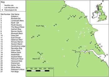
Yorkshire and Humberside additionally presents an ideal study area for the context of human–environment interaction across the Mesolithic–Neolithic transition, as parts of the region are amongst the most intensively investigated of the United Kingdom in terms of detailed paleoenvironmental research. In particular, North Gill on the North York Moors (Figure 1), has been the focus of highly detailed and influential palynological studies over the last four decades (e.g. Simmons Reference Simmons1969, Reference Simmons2003; Simmons and Cundill Reference Simmons and Cundill1974; Simmons and Innes Reference Simmons and Innes1981, Reference Simmons and Innes1987, Reference Simmons and Innes1988a, Reference Simmons and Innes1988b, Reference Simmons and Innes1988c, Reference Simmons and Innes1988d, Reference Simmons and Innes1996a, Reference Simmons and Innes1996b, Reference Simmons and Innes1996c, Reference Simmons and Innes1996d; Simmons et al. Reference Simmons, Turner and Innes1989; Innes and Blackford Reference Innes and Blackford2003; Turner et al. Reference Turner, Innes and Simmons1993; Innes et al. Reference Innes, Blackford and Rowley-Conwy2013; Albert and Innes Reference Albert and Innes2015). In this paper we review the available evidence for the elm decline in Yorkshire and Humberside, producing new chronological estimates for the palaynological signals for this event across the region, and compare these to new evidence for the end of the Mesolithic and start of the Neolithic in the region.
Paleoenvironmental study sites from the region. Selected late Mesolithic and early Neolithic sites with robust 14C chronologies (Griffiths Reference Griffiths2014a, Reference Griffiths2014b) are also shown. Analyses are detailed below and in the supplementary material.

Method
Site Selection
Eighteen paleoenvironmental sequences from the main study region with 14C dates predating 3300 cal BC were identified across Lincolnshire, through Humberside and the North Yorkshire Moors (Figure 1). The sequences were recovered from a range of depositional environments including blanket peat, intertidal, and floodplain peats. Some intensively investigated sites have been excluded from analysis, for example the previous chronological modeling of pollen records from the lowland raised mires of Hatfield and Thorne Moors, which demonstrated that declines in elm can be assigned to broader clearance of woodland during the Bronze Age (Chapman and Gearey Reference Chapman and Gearey2013). To the west of the main study region a series of complementary sequences was identified for comparison. These were Gransmoor (Beckett Reference Beckett1975), White Moss and Eshton Tarn (Bartley et al. Reference Bartley, Jones and Smith1990), Rishworth Moor (Bartley Reference Bartley1975), Robinson’s Moss (Tallis and Switsur Reference Tallis and Switsur1990), and Soyland Moor (Williams Reference Williams1985). These sequences were selected to provide upland contrasts with the predominantly lowland Yorkshire and Humberside examples, and to provide context for the important South Pennine Mesolithic landscape around March Hill (Griffiths Reference Griffiths2014a).
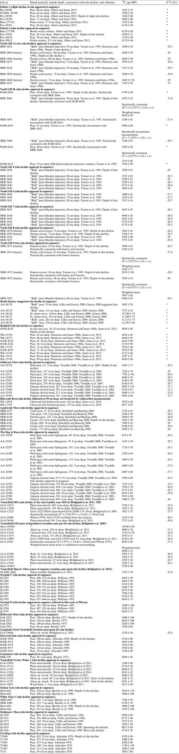
The majority of the dated samples comprise slices of “peat” or other sediment (Table 1 and supplementary material). 14C measurements on “peat” can be accomplished by dating different chemical fractions, most commonly the “humin” (the alkali and acid insoluble material) and “humic” acid fractions (the alkali soluble and acid insoluble material), or macrofossils extracted from peat samples. Generally shortlife, single entity, terrestrial plant macrofossils, which might have grown in situ at the time of the peat formation are deemed preferable (Bayliss et al. Reference Bayliss, Bronk Ramsey, Cook, van der Plicht and McCormac2008; cf. Griffiths et al. Reference Griffiths, Sturt, Dix, Gearey and Grant2015). As we shall note below, the different natures of the dated materials adds another issue in terms of providing accurate estimates for variability of the timing of the elm decline in the region.
Radiocarbon results associated with sites with indications for elm declines in the study area. The symbol * denotes that the information is not published.

Bayesian Modeling
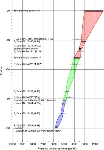
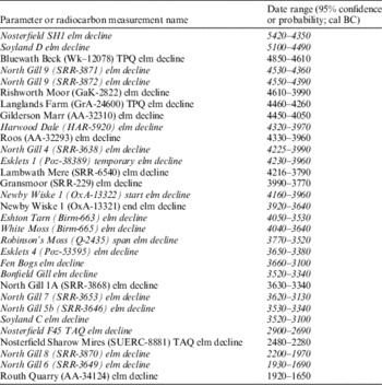
For the majority of the sites (see Table 2, Figure 2, and supplementary material), models of 14C dates from pollen sequences that include evidence for the elm decline have been produced using the program OxCal v4.1 (Bronk Ramsey Reference Bronk Ramsey1995, Reference Bronk Ramsey1998, Reference Bronk Ramsey2008, Reference Bronk Ramsey2009) and IntCal13 (Reimer et al. Reference Reimer, Bard, Bayliss, Beck, Blackwell, Bronk Ramsey, Grootes, Guilderson, Haflidason, Hajdas, Hatte, Heaton, Hoffmann, Hogg, Hughen, Kaiser, Kromer, Manning, Niu, Reimer, Richards, Scott, Southon, Staff, Turney and van der Plicht2013). For each of these sequences a model was constructed that assumed that the sediment accumulation process is an inherently random or a “Poisson” process (the P_Sequence function in OxCal v4; Bronk Ramsey Reference Bronk Ramsey2008; cf. Blaauw and Christen 2011). Our models make allowances for changing sediment accumulation rates, by including details of the interfaces between lithological units where these were specified in the original publications (using the OxCal Boundary parameter, developing the approach of Lee Reference Lee2012). Deposit models were implemented to allow for flexibility in the estimation of the formation of the sediment over the depth of the core, by averaging values of k (the rigidity of the model) between 0.01 and 100 cm–1, which should provide a robust model for any sedimentary sequence (Bronk Ramsey and Lee Reference Bronk Ramsey and Lee2013:723). The interpolation rate was set to 1. By defining the lithological units using Boundary parameters, and with the relatively limited data per unit, the effect in practice in many sequences is that the deposition rate within different units will appear fairly constant. An example of the deposition modeling is shown in Figure 2 with other models presented in the supplementary material, the modeling approach is described in the text, and selected output ranges for the elm decline are given in Table 2.
An example of the type of deposition model produced during this analysis using the results from Bonfield Gill. As with the other modeling approaches here the results have been analyzed using the deposition notation P_Sequence(“Bonfield Gill”,1,1,U(-2,2))...

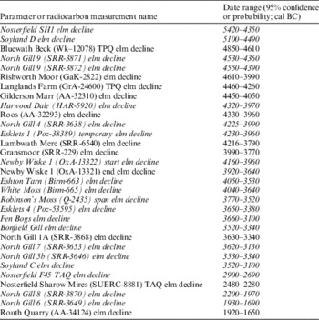
Key posterior density estimates (in italics; see models in supplementary materials and Figure 2) or calibrated radiocarbon dates calculated in this paper. All are quoted at 95% probability or confidence in years cal BC.
For “humin” and “humic” acid measurements from the same horizons statistically consistent results were combined (Ward and Wilson 1978). Where there were age inversions or samples from the same depth were not statistically consistent, formal outlier analysis was used to identify 14C results that were removed from the models (Bronk Ramsey Reference Bronk Ramsey2009:1024). Results not included as active likelihoods are indicated by the “?” sign in the model figures (Figure 2 and supplementary material). Estimates for the timing of the elm declines in each sequence have been produced using the Date parameter at the appropriate depths quoted in the original publication reports, or depths suggested in this analysis (see Tables 1 and 3).
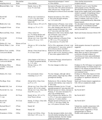
Summary of palynological signal and associated “events” at Ulmus decline for sequences with chronological models relevant to period up to 3400 cal BC (not including The Bog at Roos and Gilderson Marr). Note: Pollen percentage figures based on variable sums: North Gill sites (Turner et al. Reference Turner, Innes and Simmons1993) expressed as percentage TLP-Corylus, Alnus and Salix, except Esklets (%Arboreal pollen minus Corylus), Bluewath Beck (%Arboreal pollen minus Corlyus and Alnus), Robinson’s Moss (% Arboreal Pollen), Gransmoor (%Arboreal pollen minus Tilia). Site references: Bonfield Gill (Simmons and Innes 1988; Innes et al. Reference Innes, Blackford and Rowley-Conwy2013), Bluewath Beck (Innes et al. Reference Innes, Blackford and Rowley-Conwy2013), Esklets (Albert and Innes Reference Albert and Innes2015), North Gill Sites (Turner et al. Reference Turner, Innes and Simmons1993), Newby Wiske and Langland’s Farm (Bridgland et al. Reference Bridgland, Innes, Long and Mitchell2011), Rishworth Moor (Bartley Reference Bartley1975), Robinsons Moss (Tallis and Switsur Reference Tallis and Switsur1990), White Moss and Eshton Tarn (Bartley et al. Reference Bartley, Jones and Smith1990), Gransmoor (Beckett Reference Beckett1975).

RESULTS
From the region, several sites reviewed did not produce clear evidence for “elm declines” and are not discussed further (see supplementary material). Twenty-nine sites produced evidence for the elm decline with associated 14C dates, although as we shall see in the discussion below, there is considerable variation in the timing of these events.
The critical factor in the estimate for the timing of elm decline signals in most of these cases is not the modeling approach employed, but the nature of the dated samples and their associations with the paleoenvironmental events of interest (see discussion below). An important aspect of this is how and where the original analysts identified the elm decline in a given sequence, which is in large part dependent on the sampling interval employed (Table 3). Comparison of different palynological records can be complicated by the fact that analysts may adopt different approaches to producing pollen sums (see also Parker et al. Reference Parker, Goudie, Anderson, Robinson and Bonsall2002:3). For the sites discussed in this paper, the pollen summing approach varies from total land pollen (%TLP), to percentage total arboreal pollen (%AP), to total land pollen minus Corylus, Alnus, and Betula (at the North Gill sites; see Table 3). With the exception of two sites, the elm decline is comparatively clear in all the records, although there is some variation in terms of the apparent rapidity of the event (see discussion below).
For the sites of Bluewath Beck and Gilderson Marr the elm decline events are not estimated using deposit models, as in both sequences the elm decline pollen signals were not bracketed by 14C measurements. For Bluewath Beck the measurement Wk-12078 (5879 ± 40 BP) provides a terminus post quem for the elm decline signal, which is of limited use in unpicking the timing of the elm decline at this site. For Rishworth Moor (Gak-2822), Eshton Tarn (Birm-663), Gransmoor (SRR-229) single results estimate the elm decline at each site. A single result from Langlands Farm (GrA-24660) provides a terminus post quem for the elm decline at this location. From Sharow Mire, a result (SUERC-8881) from the base of the sequence provides a terminus ante quem for the elm decline at this sample location; this result is inconsistent with another from this sample depth (SUERC-8885) and the robustness of either of these results’ association with the elm decline is unclear.
From the Nosterfield sites of F45 and SH1, the models published in Bridgland et al. (Reference Bridgland, Innes, Long and Mitchell2011) were adapted. For F45, the three results recovered from the lowest part of the sequence have not been included as actively likelihoods in the model (Beta-143456; GrA-25355; OxA-13530); these include very early Holocene results which do not concur with the palynological evidence that the start of the sequence post dates the elm decline, and a result (GrA-25355) which is too early for the position in the sequence. An estimate for the start of the formation of deposits in the sequence provides a terminus ante quem for an elm decline here. The model for the Nosterfield SH1 sequence does not include OxA-13225 as an active likelihood as this result is too old for its position in the sequence.
The results from the North Gill sample site NG1A presented multiple modeling solutions; in this case the statistically consistent (T’=0.0; T’5%=3.8; df=1) 14C results from the elm decline deposit are used to estimate its timing (Figure 3). Similarly, the calibrated 14C results from the elm decline horizons from Routh Quarry, Gilderson Marr, Lambwath Mere and The Bog at Roos are included in Figure 3. The results from Lambwath Mere, Gilderson Marr, and the Bog at Roos produced multiple potential modeling options, with these sequences producing measurements with multiple 14C age inversions, and too few measurements to be able to suggest which results were best used to constrain the timing of the elm decline. The results estimating these events were included in the discussion presented below. The remaining sites (Soyland D, Soyland C, Harwood Dale, North Gill 4, Esklets 1, Newby Wiske 1, White Moss, Robinson’s Moss, Fen Bogs, Bonfield Gill, North Gill 9, North Gill 7, North Gill 5b, and North Gill 6) were all modeled as outlined in Figure 2 (and see supplementary material).
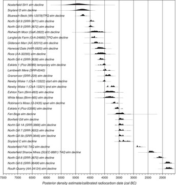
Estimates from the elm decline for all the sequences that modeled, and calibrated 14C dates from Rishworth Moor, North Gill A1, Routh Quarry, Gilderson Marr, Roos, Bluewath Beck, Gransmoor, Sharow Mires (providing a terminus ante quem for the decline), Lambwath Mere and Langlands Farm (providing a terminus post quem for the decline).

Of the results shown in Figure 3, it is apparent that only some have produced middle Holocene chronologies. The nature of the early elm declines is also variable. For example, at North Gill sample site North Gill 9 two “elm declines” were recorded in the pollen record, while at Esklets 1, a “temporary elm decline” was noted by Albert and Innes (Reference Albert and Innes2015), although this appears to be associated with a hiatus in peat accumulation. We shall return to these points in the discussion below.
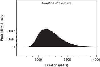
From the evidence we have assembled here, elm declines are associated with 14C measurements from the mid-fifth millennium to the first millennium cal BC. The total duration of activity represented by these measurements is estimated in Figure 4 as 2900–3620 yr (95% probability; or 2990–3320 yr 68% probability; duration elm decline). The temporal variability of “the elm decline” emphasizes the importance of how paleoenvironmental events are defined. In paleoenvironmental contexts, the “elm decline” can be defined both as a signal from proxy data and chronologically as an event—which we can find in the archaeological record—at or close to the Mesolithic–Neolithic transition. If an event has both chronological and paleoenvironmental definition, we begin to reify our data with our archaeological assumptions. In this case, some scientific chronological data become regarded as “chronologically acceptable” and some as not. These approaches to data are especially important when we begin to look at processes, both in terms of local process of vegetation change and in terms of human–environment interaction. This is especially so if we seek to explore the potential for correlation with cultural practices which might be equally difficult to define (Figure 5).
The total duration of activity associated with “elm decline events” shown in Figure 3.

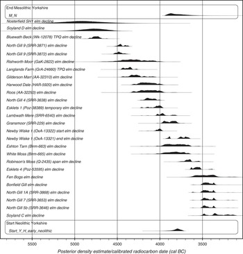
Detail of the estimates for the earlier prehistoric elm decline and estimates for the start of the Neolithic in Yorkshire and Humberside, and the latest Mesolithic activity in this part of the world.

The elm decline is traditionally thought to have been associated with Neolithic activity in Britain, or to have occurred after the start of Neolithic activity (Whitehouse et al. Reference Whitehouse, Schulting, McClatchie, Barratt, McLaughlin, Bogaard, Colledge, Marchant, Gaffrey and Bunting2014). In this region, both the elm declines represented in North Gill 9 and the elm declines sampled in Nosterfield SH1, Soyland D, Rishworth Moor, Langlands Farm, Gilderson Marr, Harwood Dale, Roos, North Gill 4, Esklets 1, and probably Lambwath Mere and the start of the decline at Newby Wiske occurred before the end of the Mesolithic in the region (parameter M_N in Figure 5; calculated and discussed in Griffiths Reference Griffiths2014a, Reference Griffiths2014b) and before the start of the earliest available evidence for the start of the Neolithic in the region (parameter Start_Y_H_early_Neolithic in Figure 5; calculated and discussed in Griffiths Reference Griffiths2014a, Reference Griffiths2014b). In contrast for example, it is 90% probable that the start of the Neolithic in Yorkshire and Humberside (Start_Y_H_early_Neolithic) occurred before the elm decline recorded at Bonfield Gill (Bonfield Gill elm decline; Figure 5). Other elm declines occurring after the start of the Neolithic include those at Esklets 4, Fen Bogs, North Gill 1A, North Gill 7, North Gill 5b, and Soyland Moor C.
These results demonstrate that the elm decline across Yorkshire and Humberside cannot be regarded as rapid or synchronous (cf. Parker et al. Reference Parker, Goudie, Anderson, Robinson and Bonsall2002) and is not necessarily closely associated with the Mesolithic–Neolithic transition in the region. This applies even if the later elm declines are excluded from discussion—there is evidence for different estimates for elm declines across the intensively studied location of North Gill for example. The calibrated 14C dates and posterior density estimates from the North Gill sites indicate the elm decline took place over 2540–2820 yr (95% probable; or 2600–2740 yr 68% probable), across a sample area of only several hundred meters; our evidence for the timing of this “event” shows considerable variability even here. Of the North Gill sequences, North Gill 1A, North Gill 5b, and North Gill 7 have produced very similar estimates for the elm decline (see Table 2). In classic palynological terms, this could represent the second sustained reduction in elm pollen frequencies following the recovery of elm percentages from a first elm decline (Hirons and Edwards Reference Hirons and Edwards1986:138), or this could derive from a hiatus in deposit formation for which there is not evidence in the stratigraphy or pollen proxies. There remain however very different estimates from North Gill 9 and North Gill 4 that should be interrogated in any discussion of the elm decline (Table 1); developments in precision mean it is not simply enough to suggest these results are contemporaneous or “noise.” These data may inform on process. An important aspect of the studies at North Gill is the high-resolution pollen-sampling interval adopted (Table 3), which means that the elm decline can be precisely located. However, it can also be noted that the expression or form of the decline varies, with the reduction in Ulmus at abrupt (over 1-cm sample interval) at North Gill 1A, North Gill 4, North Gill 6 and North Gill 9, to rather less so (resolved over 4–6-cm sample intervals) at North Gill 5b, North Gill 7 and North Gill 9.
The original analysts at North Gill concluded that this spatial and chronological variation could be attributed to each location having a “different management history between 9000-6000 BP...” with Mesolithic impacts (burning, lopping of trees) and climatic deterioration affecting the quality of the local soils and hence the ability of elm to regenerate after each impact “event” (Turner et al. Reference Turner, Innes and Simmons1993:646). Disease is implicated as a causal factor in this scenario but it is suggested the reason that adjacent sites (for example, sites North Gill 7 and 9 are ca. 50 m apart) do not record synchronous declines is that those pollen sequences were located close to soils with optimal nutrient status supporting elm populations that were better able to recover following the initial impacts of disease. In other words, the elm decline at North Gill is not strictly regarded as asynchronous and must be understood as a hyper-local process, with diseased trees rapidly replaced at certain locations. Hence the impact of this “process” is essentially “palynologically invisible” during the initial onset. In this scenario, the later declines demonstrate the subsequent, palynologically identifiable, impact on local elm populations.
An associated aspect of this hypothesis is the assumption that for such apparently divergent vegetation histories, the relevant source area of pollen (RSAP; Sugita Reference Sugita1994) for the sampling locations must have been very small. In the case of those sequences which are relatively close to each other (North Gill 8 is less than 40 m north of North Gill 1A) but show chronologically disparate declines, this would imply the RSAP for the sampling sites must have been at the very lowest end of the estimates for forest hollows (ca. 2 m diameter) calculated by Sugita (Reference Sugita1994). This hypothesis could be usefully tested further through palynological modeling approaches (e.g. Caseldine and Fyfe Reference Caseldine and Fyfe2006).
However, further investigation may simply lead to evidence for greater complexity rather than greater clarity, in which case pollen taphonomic considerations may be contributing to this picture, especially in the case of multiple sequences sampled at very fine (1-mm) intervals. Following the conclusions of the original analysts and the data presented in this paper, if the North Gill 14C estimates associated with elm decline signals are robust, then it would appear that the elm decline on the North York Moors a highly complex “event” occurred effectively on the microscale, with healthy or regenerating elms co-existing alongside areas of dead or dying elms. Such a picture is concurrent with causal mechanisms which include interaction between a disease vector, localized edaphic conditions and human impact. In this model an “elm decline” is only recognizable in the proxies once some sort of “palynological tipping point” is passed when the greater majority of elm trees within a given catchment were affected to an extent sufficient to produce a clear palynological signal (Turner et al. Reference Turner, Innes and Simmons1993: 646). In this scenario, it is possible that early, spatially restricted declines in elm would be invisible in any sequence with a relatively large RSAP. Under these conditions, the “elm decline” could theoretically have begun earlier than apparently recorded in a given sequence, with associated implications for the identification of the timing and thus the underlying cause(s) of the decline. If we propose this as hypothesis for North Gill then we must also accept that these issues identifying the start of the elm decline could exist in other similar locations.
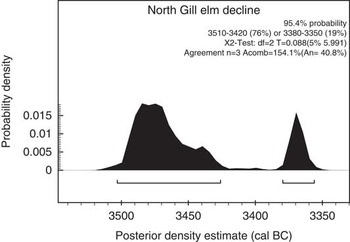
A further range of possibilities exists, including that some of the 14C measurements are not accurate estimates for the date of the elm decline in the parent contexts (cf. Brock et al. Reference Brock, Lee, Housley and Bronk Ramsey2011). It is possible, given the relatively limited numbers of 14C dates from each North Gill sequence (and especially the inconsistency of the North Gill 4 sequence), that those from North Gill 4 and 9 are not robust estimates for the elm decline at these levels. If we accept that the similarity between the estimates from North Gill samples NG4, NG5b, and NG7 represent the sustained reduction (or “elm decline proper”), and we regard this as a local “event” we can combine the posteriors from these sites to provide what may be the most robust estimate for the elm decline here (Figure 6), with the event estimated to have taken place in 3510–3420 cal BC (76% probability) or 3380–3350 cal BC (19% probability).
A combined estimate for the elm decline evidenced in North Gill cores NG4, NG5b, and NG7. This approach excludes much earlier estimates from the North Gill landscape, and we cannot be exactly certain why these variable earlier signatures were detected over such a small landscape. The 14C chronology and taphonomy of the proxies could be contributing to these earlier signals.

For sequences away from North Gill, the sampling interval—and thus the identification of the elm decline depth—adopted in the different studies could have implications for our understandings (see Table 3). This may be the case for the sequences with comparatively wide sampling intervals as at Harwood Dale and Fen Bogs, where the timing of the decline could be resolved earlier. Given the relatively low values for Ulmus in the Routh Quarry sequence, it is possible that an earlier prehistoric decline at this site falls between the sampling interval (8 cm). At other sides, aside from Esklets 4 (where the decline signal is very subdued), the reductions in Ulmus regarded as the “decline” event are pronounced and recorded across sampling intervals of a maximum of 5 cm (Rishworth) but generally no more than 2 cm, and sampling interval seems less likely to contribute to issues with the dating of the decline.
Beyond the specifics of the timing of the appearance or disappearance of different environmental proxies, the evidence from this case study concerning how we approach paleoenvironmental events has more significant implications. Our interpretation of what the elm decline is—at its most extreme whether we conceive of this signal as “event” or “process”—has implications for how we interpret the available data and the range of possible causal processes we are willing to entertain. If we define the elm decline as an event with the same chronological signature in a determined study area, then we exclude data that are by this definition “noisy.” However, these data might actually be telling us something important about the inappropriateness of our approaches, they might in fact be indicative of a complex process, or at least a process with paleoenvironmental proxies with complex, poorly understood taphonomies. This then has implications for our causal narratives and our willingness to move between the specific and the general, and it is directly impacted by the scale of analytical approach taken.
DISCUSSION
Palynological Conclusions
In this paper we have analyzed the 14C chronologies associated with the elm decline in palynological records from Yorkshire and Humberside. In order to identify possible causes of this “event” and to establish possible relationships with human activity as demonstrated by the archaeological record (e.g. Innes et al. Reference Innes, Blackford and Rowley-Conwy2013), we require robust chronological data. In all paleoenvironmental research, an understanding of the taphonomic processes that resulted in the formation of assemblages that we analyze is essential. In the case of every elm decline—or any other palynological “event”—we need to interrogate our proxies, to determine what they actually mean in terms of environmental reconstruction and the archaeology of people. It is only when we have rigorously examined our proxies in this way that we can begin to talk about processes, or the nature of different elm declines (cf. Smith and Pilcher Reference Smith and Pilcher1973 on “rational limit” and “empirical limit”; Hirons and Edwards Reference Hirons and Edwards1986 on definition of the elm decline). The importance of increased precision that Bayesian modeling allows, should include an unpicking simplistic causal narrative resulting from chronologies which suck in or smear anthropogenic and paleoenvironmental events (cf. Baillie Reference Baillie1991).
Without critically thinking about what our proxies mean, and what our analytical terms and scales impose on our data there is a real danger that paleoenvironmental events become reified from concepts into things that are identifiable in the archaeological record. In such cases, analysis can become focused on identifiable concepts rather than the specificity of paleoenvironmental conditions at different study sites. In this case, paleoenvironmental events can take on “mythic” properties, where the abstraction from evidence to causal process becomes so complete that the concepts are no longer helpful in terms of critically engaging with the available evidence. Researchers look for “the elm decline” because it has taken on an analytical, intellectual identity. Looking for “the elm decline” or other comparable paleoenvironmental events puts the interpretation before the data. Rather than characterizing the pattern of vegetation change at individual sample sites, seeking preconceived paleoenvironmental responses starts to interpret data and applies a causal narrative prior to analysis. This is what Lowe and Higham (Reference Lowe and Higham1998) referred to as “coherent myths,” and to which we will return later.
Archaeological Questions
In Yorkshire and Humberside, the latest Mesolithic activity has been identified on Pennine upland sites such as March Hill and South Haw (Spikins Reference Spikins2002; Griffiths Reference Griffiths2014a, Reference Griffiths2014b). Looking at the earlier results, including those from North Gill 9, North Gill 4, Nosterfield SH1, Soyland D, Rishworth Moor, Langlands Farm, Gilderson Marr, Harwood Dale, Roos, and probably Lambwath Mere and the start of the decline at Newby Wiske (Figure 3), these signals could be indicative of temporary disturbances to the local vegetation including declines in elm of the sort noted by Albert and Innes (Reference Albert and Innes2015) at Esklets 1. This takes place when there is clear evidence in upland Yorkshire for late Mesolithic hunter-gatherer populations, including those returning repeatedly to what has been glossed as “persistent places” (cf. Barton et al. Reference Barton, Berridge, Walker and Bevins1995) such as March Hill. On this basis alone these pre-Neolithic disturbances could result in part at least from Mesolithic human–environment interactions.
The next evidence for elm declines in Yorkshire and Humberside is represented by a series of distributions centering on 3500 cal BC, after the first evidence for Neolithic material culture and practices in this region (Griffiths Reference Griffiths2014b). The similarity of the estimates from Fen Bogs, North Gill 1A, North Gill 7, North Gill 5b, Bonfield Gill, and Soyland C are notable; that for the elm decline at Esklets 4 is somewhat earlier, although this is described as “a low scale event” (Albert and Innes Reference Albert and Innes2015:370). This could be indicative of environmental disturbance associated with the wide-ranging adoption of agriculture, post-dating as it does the timing of the appearance of cereals across Britain and Ireland (Griffiths in prep.) although none of these records are regarded as demonstrating clear palynological evidence for Neolithic clearance or farming (Table 3). This said with the exception of Soyland C all these sites—Esklets, Bonfield Gill, and North Gill—are located in a relatively circumscribed area of the uplands of the North Yorkshire Moors. The similarity of these estimates, and that from Soyland C (a Pennine site), suggests that there might be some coherence in the post-Neolithic elm decline in the uplands of Yorkshire. It remains unclear how indicative these records are of wider environmental changes, especially given the relatively limited sample of lowland environments available within the region.
It has been suggested that the pollen record from Bonfield Gill indicates the use of fire to manipulate woodland structure during the Mesolithic, with disease potentially weakening trees subsequent to an episode of “forest farming” during the earlier Neolithic (Innes et al. Reference Innes, Blackford and Rowley-Conwy2013). In this context, it is perhaps most telling that aside from Newby Wiske (Bridgland et al. Reference Bridgland, Innes, Long and Mitchell2011), none of the original interpretations of the pollen records unequivocally implicate human activity as a dominant factor, suggesting potentially highly complex processes which even detailed analytical approaches may not necessarily reveal (cf. Batchelor et al. 2014). Overall, if the elm decline was associated even in part with the impact of human activity it is clear that this process began prior to the introduction of farming in the study area. Later coherent signals for an elm decline from upland sites across Yorkshire may be associated with a geographical expansion of Neolithic practices into areas that were witness to the very latest Mesolithic practices.
CONCLUSION
This paper has provided new analysis of the timing of the elm decline in Yorkshire and Humberside, and compared this with evidence for Mesolithic and Neolithic material culture. We emphasize the importance of analyzing the available data, and variability in that data in order to develop critical chronologies. We suggest that the fine-grained chronologies offered by Bayesian modeling afford new opportunities for approaching human–environment interaction, and to explore the subtleties of these processes; “noise” or variability in the timing and tempo of “events” may actually be informing us about the nature of the underlying processes. We should not however assume that more precise chronologies, in and of themselves, will provide a catch all causal “answer” if the models and approaches within which we frame our data are not sufficiently flexible.
In terms of the elm decline in Britain, without robust approaches to the chronology of latest Mesolithic and earliest Neolithic material culture and practices, understanding human involvement in these processes will inevitably be difficult, especially when people involved in Mesolithic and Neolithic lifeways might have been involved in complex human–environment interactions. Drilling down into the detailed evidence for environmental and anthropogenic change is essential to get beyond simple correlation:causation models. Without this, “events” such as the elm decline risk taking on a mythic property (Lowe and Higham 1998), becoming what we might regard as chronological moveable causal feasts that are marshaled to cover insufficient data. We hope this paper demonstrates the inherent value in producing robust and quantifiable approaches to paleoenvironmental chronologies. Noisy, complex data may be intrinsically interesting in terms of archaeological narratives; we are doing a disservice to our hard-won evidence if we do not attempt to engage with this complexity.
Acknowledgments
Charlotte Bryant of NERC is thanked for detailing sample pretreatment and measurement and δ13C values. Two anonymous reviewers are thanked for their comments on an earlier draft.
Supplementary material
For supplementary material/s referred to in this article, please visit https:/doi.org/10.1017/RDC.2017.73