Implications
There is a growing demand for tilapia fillet, mostly in markets with higher product standards. Moreover, it is expected in the near future that these markets may be interested in processed products too. Therefore, meat yield can become an objective for genetic improvement in tilapia breeding programs. Fillet traits cannot be directly used for selection of replacement animals. But, by selecting for correlated traits, like morphometric ones, breeding programs can easily practice selection. The results of this research indicate the possibility of achieving indirect genetic gains for fillet weight by the selection of morphometric traits but low efficiency for FY if compared with direct selection.
Introduction
The growing international demand for tilapia products is a major factor driving the genetic improvement of production efficiency for this species. Also, the product which shows a higher increase in trades is frozen tilapia fillet (Food and Agriculture Organization, 2016, Supplementary Figures S1 and S2). Moreover, the authors expect that in the near future, market interest in processed products may increase, perhaps following the same evolution of swine and poultry production. Therefore, meat yield, and more precisely carcass and fillet yields (FYs), are of extreme importance for the tilapia product chain and can become objectives for genetic improvement in tilapia breeding programs.
Some problems normally arise when selecting for traits that are a ratio of other traits. One is that those traits generally are less variable and consequently present lower heritability (Simm et al., Reference Simm, Smith and Thompson1987), thus it may be of interest to search for correlated traits to be used as selection criteria for the genetic improvement of the target trait. Moreover, fillet traits cannot be directly used for selection of replacement animals, as slaughter is required in order to measure those traits. By selecting for correlated traits, breeding programs can easily practice mass selection. Motivated by the benefits of indirect selection, several studies have reported estimates of phenotypic and genetic correlations between carcass and morphometric traits for several fish species (Cibert et al., Reference Cibert, Fermon, Vallod and Meunier1999; Bosworth et al., Reference Bosworth, Holland and Brazil2001; Rutten et al., Reference Rutten, Bovenhuis and Komen2005a; Nguyen et al., Reference Nguyen, Ponzoni, Abu-Bakar, Hamzah, Khaw and Yee2010; Fernandes et al., Reference Fernandes, Silva, Alvarenga, Teixeira, Silva, Alves, Salles, Manduca and Turra2015).
Morphometric traits, also known as body measurements, describe the body shape of fish. This shape can differ both between and within species and are related to BW and perhaps FY as well (Cibert et al., Reference Cibert, Fermon, Vallod and Meunier1999; Bosworth et al., Reference Bosworth, Holland and Brazil2001). However, recent studies in Nile tilapia reported divergent results regarding the use of morphometric traits to promote indirect genetic gains in FY. Literature results range from promising (i.e. high genetic correlation between body measurements and FY; Rutten et al., Reference Rutten, Bovenhuis and Komen2005a), to discouraging (i.e. low to moderate genetic correlations; Nguyen et al., Reference Nguyen, Ponzoni, Abu-Bakar, Hamzah, Khaw and Yee2010).
Until recently, the majority of studies focusing on genetic correlations between traits of interest in Nile tilapia, or other fish species, used multiple trait models to estimate genetic correlations. However, random regression models (RRM) offer an alternative approach. In the multiple trait contexts, RRM are able to describe the relationships between traits across any continuous covariable. Therefore, RRM may be a powerful tool for identification of an optimal age to measure and select animals in order to achieve a maximum indirect response to selection. However, there are few studies in fish that have employed RRM. Also, we could not find any study of morphometric traits for indirect selection of fillet traits on a wide range of time, only the study of Turra et al. (Reference Turra, Oliveira, Valente, Teixeira, Prado, Melo, Fernandes, Alvarenga and Silva2012b) reported RRM approaches for carcass traits and BW, but no morphometric traits were analyzed. Therefore, the objective of the present study was to investigate the genetic relationship and correlated response efficiency (CRE) to selection between body measurements and fillet traits throughout 106 to 245 days of growth and to evaluate the use of indirect selection for improvement of fillet weight (FW) and FY in Nile tilapia.
Material and methods
Breeding strategies
The experiment was conducted at the Aquaculture Laboratory of the Veterinary School at the Federal University of Minas Gerais (UFMG), Brazil. The population used in this study was the laboratory’s Chitralada Nile tilapia strain. This strain was introduced from Thailand to Brazil in 1996 and has become a popular farmed strain across the country. The UFMG stock originated from a commercial hatchery in the state of Minas Gerais, which conducts a breeding program based heavily on selection for growth rate.
In all, 72 full-sib families were produced by mating 36 males and 72 females that were randomly sampled from 100 males and 300 females. Each fish was tagged with a unique passive integrated transponder device. Turra et al. (Reference Turra, Oliveira, Valente, Teixeira, Prado, Alvarenga, Melo, Felipe, Fernandes and Silva2012a and Reference Turra, Oliveira, Valente, Teixeira, Prado, Melo, Fernandes, Alvarenga and Silva2012b) describe a more detailed process for these specific families’ production.
Data recording
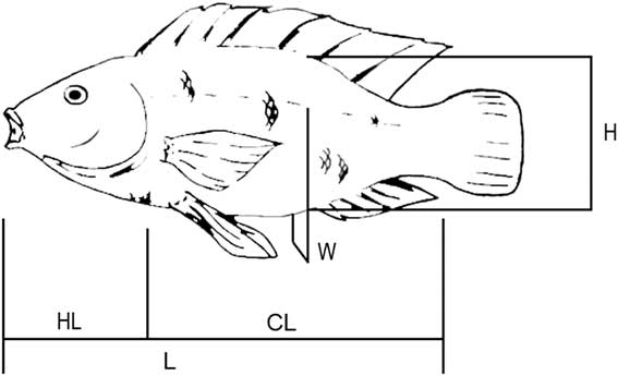
Each fish was individually weighed and measured a maximum of six times. The first weight (g) and body measurements (mm) were taken at the time of tagging. The body measurements taken were: standard length (L) and head length (HL) for the estimation of corrected length (CL=L−HL; adapted from Rutten et al., Reference Rutten, Bovenhuis and Komen2004), width (W) and height (H) (Figure 1). Height was taken from a perpendicular line at the anus (anterior of the first ray of the anal fin). Width was the largest point taken at the same perpendicular line. These measurements were chosen following the results of Diodatti (Reference Diodatti2006), where the highest phenotypic correlations with FY were between body measurements taken at this perpendicular line.
Body measurements taken on each fish: length (L), head length (HL), corrected length (CL), height (H) and width (W) (adapted from Rutten et al., Reference Rutten, Bovenhuis and Komen2004).

Records were taken across the full range of the growth period from 106 to 245 days of age. The time between measurements varied among tanks from 14 to 28 days. These variable and irregular intervals were chosen to obtain a more distributed data set of body measurement observations throughout the entire range of ages, and therefore create a data set more suitable for random regression analysis. At the sixth recording, all the remaining fish of each family were measured and slaughtered to obtain FW and FY. Earlier sex determination of each fish was confirmed during the evisceration process.
At each time of measurement, fish were randomly selected from each family and harvested in order to record FW and yield. To avoid handling stress, fish were previously anesthetized by cold narcosis. As family size was variable, the number of harvested fish was different among families as well. Nevertheless, around 10 fish/family were available for the last harvest date. In families with more than 30 identified fish, four were randomly selected to be harvested at each of the five evaluation periods. In families with 22 to 30 fish, three were randomly selected. In those with 18 to 22 fish, two were randomly selected. Families ranging from nine to 17 identified individuals had one member randomly selected in each period, assuring at least four fish for the last measurement.
Fillet weight refers to a fillet without scales from the left side and with intact ribs and skin. The fillet was then cut through the ventral line and its weight was multiplied by two. One person performed both procedures. Fillet yields were expressed in relation to a fish’s live weight.
Statistical analysis
The data set was divided into two subsets. The first contained a total of 8758 records for each body measurement. This first data set containing repeated measures as fish had body measures taken in more than one point in time prior to slaughter. The second data set contained 2042 records for each trait. This second data set consist only of the body measurements and fillet traits collected at harvest, thus each fish has only one data point for each trait, but the data set has points distributed across the whole period. The first data subset was used to estimate parameters for BW (already published by Turra et al., Reference Turra, Oliveira, Valente, Teixeira, Prado, Alvarenga, Melo, Felipe, Fernandes and Silva2012a) and body measurements via univariate analysis. The second data subset was used to estimate genetic correlations, heritabilities and resulting CRE between body measurements and fillet traits.
In order to describe body measurements (data subset one analysis), four different models were used. The models differed by inclusion or exclusion of a random family effect (Martínez et al., Reference Martínez, Neira and Gall1999; Pante et al., Reference Pante, Gjerde, McMillan and Misztal2002). This approach was an attempt to account for non-additive genetic effects, additive maternal genetic effects, and common environmental effects. The models also differed by considering homogenous or heterogeneous residual variances (10 classes, with 14-day intervals). Each of the models included sex and tank as fixed effects and additive direct and permanent environment as random effects. The Akaike information criterion (AIC) proposed by Akaike (Reference Akaike1973) was used to compare the different RRMs.
Functions of third order orthogonal Legendre polynomials were employed to describe both fixed and random effects. The decision to use polynomials of third order was based on preliminary studies and the Supplementary Table S1 illustrate the relative importance of regression coefficients for the additive genetic effect from the single trait model for FY assuming homogeneity of residual variance. The model that included a family effect with heterogeneous residual variance is described in matrix notation as:
 $$y{\,\equals\,}Xb{\plus}Z_{1} u{\plus}Z_{2} p{\rm {\plus}}Z_{{\rm 3}} f{\plus}{\rm e}$$
with the following assumptions:
 $$\eqalignno{ & E\left( y \right){\,\equals\,}Xb \cr & E\left( {Z_{1} u} \right){\,\equals\,}E\left( {Z_{2} p} \right){\,\equals\,}E\left( {Z_{3} f} \right){\,\equals\,}E\left( e \right){\,\equals\,}0 $$
and the variance of y is:
 $${\it V}\left( {\it y} \right){\,\equals\,\,}{\it Z}_{1} \left( {{\it A}\,\otimes\,{\it G}} \right){\it Z}_{1}^{\prime} {\plus}{\it Z}_{2} \left( {{\it I}_{{\it h}} \,\otimes\,{\it P}} \right){\it Z}_{2}^{\prime} {\plus}{\it Z}_{3} \left( {{\it I}_{{\it m}} \,\otimes\,{\it F}} \right){\it Z}_{3}^{\prime} {\plus}{\it I}_{{\it n}} \sigma _{{{\it ek}}}^{2} $$
where
y
is the vector of observations,
b
the vector containing regression coefficients of fixed effects;
u
,
p
and
f
the vectors containing random regression coefficients of additive genetic, permanent environmental and family effects, respectively;
X
,
Z
1
,
Z
2
and
Z
3
the design matrices related to vectors
b
,
u
,
p
and
f
, respectively, which include Legendre polynomials obtained as functions of age; and
e
the vector of random residual effects. Furthermore,
A
is the numerator relationship matrix,
G
,
P
and
F
are 3×3 covariance matrices of random regression coefficients associated with additive genetic, permanent environmental, and family effects, respectively;
 $$\sigma _{{{\bf ek}}}^{{\bf 2}} $$
is the residual variance for class
k
;
I
are the index matrices of orders
h
,
m
,
n
;
h
the number of animals with observations;
m
the number of females having progeny;
n
the total number of observations; and ⊗ is the Kronecker product.
The elements of matrices G, P and F as well as
 $$\sigma _{{{\bf ek}}}^{{\bf 2}} $$
were estimated using the WOMBAT software (Meyer, Reference Meyer2011), which utilizes a restricted maximum likelihood procedure. These estimators were applied to covariance functions and allowed the representation of the covariance structure associated with the random effects for the range of ages considered in the analyses. These structured (co)variances permit the estimation of random effects for any combination of ages, as well as obtaining heritability estimates. The genetic covariance between transformed ages
i
and
j
(
σ
AiAj
) can be estimated as:
 $$\eqalignno{ & \sigma _{{AiAj}} {\,\equals\,}Z_{{1i}} GZ_{{1j}}^{'} \cr & Z_{{1i}} {\,\equals\,}\left| {\matrix{ {\phi _{0} \left( i \right)} & {\phi _{1} \left( i \right)} & {\phi _{2} \left( i \right)} \cr } } \right| \cr & Z_{{ij}}^{'} {\,\equals\,}\left| {\matrix{ {\phi _{0} \left( j \right)} \cr {\phi _{1} \left( j \right)} \cr {\phi _{2} \left( j \right)} \cr } } \right| $$
The elements  ,
 and
 are the Legendre polynomials for intercept, linear and quadratic order for ages i and j. Additive genetic variance for each transformed age was obtained using the same formulas but considering
i
=
j
.
The permanent environmental variance was estimated following a similar approach but replacing G by P.
The genetic correlation between any two points (different ages) for the same trait within the total age interval can be estimated as follows:
 $$r_{{AiAj}} {\,\equals\,}{{Z_{{1i}} GZ_{{1j}}^{'} } \over {\sqrt {Z_{{1i}} GZ} _{{1i}}{\!}{\!}{\!}^{'} \cdot \sqrt {Z_{{1j}} GZ_{{1j}}^{'} } }}$$
The heritability at transformed age i was estimated as:
 $$h_{{Ai}}^{2} {\,\equals\,}{{Z_{{1i}} GZ_{{1i}}^{'} } \over {Z_{{1i}} GZ_{{1i}}^{'} {\plus}Z_{{2i}} PZ_{{2i}}^{'} {\plus}Z_{{3i}} FZ_{{3i}}^{'} {\plus}\sigma _{{ek}}^{2} }}$$
To obtain estimates of genetic correlations among body measurements and fillet traits, bivariate RRMs that included the same fixed, additive genetic, and family effects described earlier were used (data subset two). Bivariate analyses were used due to simplicity, to not take into account the correlation between morphometric traits and thus, to avoid problems of multicollinearity. The bivariate analyses enabled the evaluation of correlated responses for fillet traits by direct selection for body measurements. Correlated response efficiencies were estimated as:
 $${\bi E}{\,\equals\,}{\bi r}_{{{\bf xy}}} . {\bi i}_{{\bf x}} . {\bi i}_{{\bf y}} ^{{{\bf {\minus}1}}} .{\bi h}_{{\bf x}} .{\bi h}_{{\bf y}} ^{{{\bf {\minus}1}}} $$
where r xy is the correlation between traits, h x the square root of heritability and i x the selection intensity for trait x . Selection intensity for body measurements was 2.27 (3%) and 1.98 for carcass and fillet traits (6%, considering that half of the evaluated population was slaughtered for data collection).
Studying the same strain of tilapia, Turra et al. (Reference Turra, Oliveira, Valente, Teixeira, Prado, Alvarenga, Melo, Felipe, Fernandes and Silva2012a and Reference Turra, Oliveira, Valente, Teixeira, Prado, Melo, Fernandes, Alvarenga and Silva2012b) reported a significant family effect for the univariate analyses of BW, fillet and carcass traits. Therefore, it was also included for these traits in the present study. Similarly, this effect was found to be significant for morphometric measurements (Table 1). For these reasons, this random effect was included in all bivariate models.
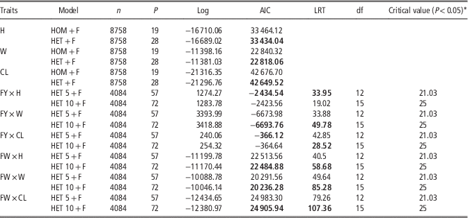
Akaike information criterion (AIC) comparison of random regression models for height (H), width (W) and corrected length (CL) when considering family effect and residual homogeneity of variance (HOM+F) or residual heterogeneity of variance (HET+F)

LRT, likelihood ratio test; FY, fillet yield; FW, fillet weight.
AIC and likelihood ratio test (LRT) comparison of bivariate random regression models for FY or FW with H, W and CL when considering a family effect and residual heterogeneity of variance with five classes (HET 5+F) or residual heterogeneity of variance with 10 classes (HET 10+F). The final model is displayed in bold.
* Critical value for the LRT test.
For each bivariate analysis, three different models were evaluated and compared by AIC and the likelihood ratio test (LRT) (Neyman and Pearson, Reference Neyman and Pearson1928). When the result obtained for AIC and LRT were different, the simplest model was chosen. The models compared considered homogeneity or heterogeneity of residual variance with five classes (of 28 days each) or ten classes (of 14 days each). The model with the better goodness of fit was chosen to estimate the genetic correlation, heritabilities and the CRE of each pair of traits.
Results
Model selection
The AIC values obtained for each model from the univariate analysis of the body measurements (data subset one) are shown in Table 1. The lower and more desirable values (better goodness of fit) were observed for the univariate models of all traits that accounted for both heterogeneous residual variance and the random family effect. These results emphasize the importance of accounting for a family effect as well as environmental changes, even in a controlled environment such as a recirculation system. For the bivariate analyses, the majority of models with 10 classes for residual heterogeneity of variance showed the lowest AIC value, in agreement with the results of the LRT tests. The exceptions were for FY with H and CL (Table 1). For these bivariate analyses, the models that accounted for family and five classes of residual heterogeneity of variances were chosen to estimate the genetic correlations, heritabilities, and CREs. As there was disagreement between AIC and LRT, choosing the simpler of the two models reduced the possibilities of overfitting.
Estimated variance ratios
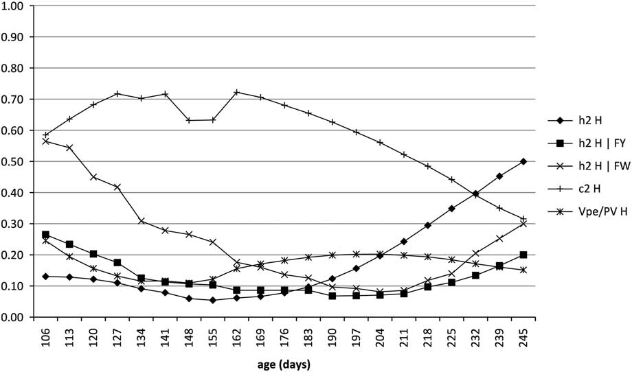
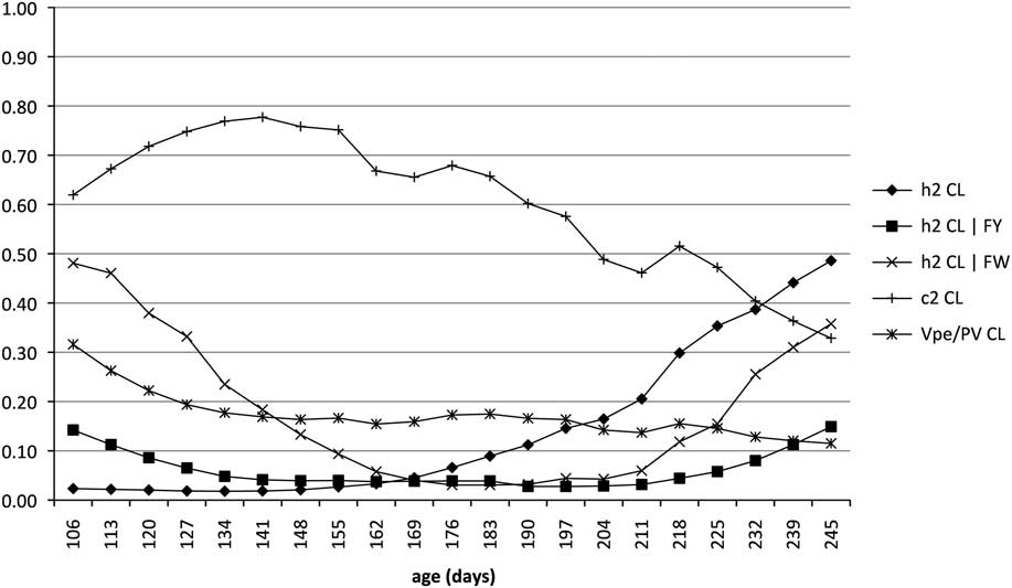
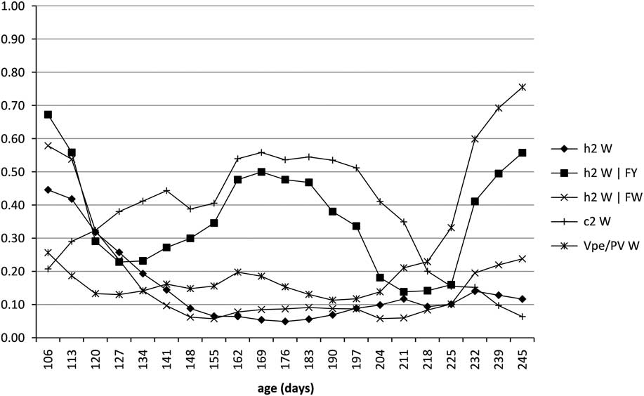
The univariate analysis for H and CL described similar curves (Figures 2 and 3), with the effect of family common environment (c 2) decreasing with increasing age. On the other hand, the estimates of h 2 increased toward the later ages for these traits. In addition, h 2 estimates from each bivariate analysis for these traits also described similar patterns (Figures 2 and 3), with the highest values estimated at 106 or 245 days of age. These results were expected as morphometric traits generally present high h 2 and are highly correlated with each other. These results are in agreement with the estimates from other studies (Rutten et al., Reference Rutten, Bovenhuis and Komen2005a; Charo-Karisa et al., Reference Charo-Karisa, Bovenhuis, Rezk, Ponzoni, van Arendonk and Komen2007; Fernandes et al., Reference Fernandes, Silva, Alvarenga, Teixeira, Silva, Alves, Salles, Manduca and Turra2015). It is relevant to note that, the univariate estimate of h 2 for W show a different curve (Figure 4), initially the values were high, decreasing to low values at ages between 148 to 180 days growing again to moderate values at the end of the studied interval. The h 2 estimates from the bivariate analyses for W were higher than univariate estimates in general, with very high estimates for ages in the middle of the studied period for the bivariate model with FY (Figure 4).
Estimates of additive genetic variance of height (h 2 H), family common environmental variance (c 2 H) and permanent environmental variance (Vpe/PV H) as ratios of the total phenotypic variance across ages. Estimates were obtained from a random regression model including a random family effect and residual heterogeneity of variance. Heritability of H, as a function of age, was estimated by a bivariate random regression model including fillet yield (h 2 H | FY) and fillet weight (h 2 H | FW).

Estimates of additive genetic variance of corrected length (h 2 CL), family common environmental variance (c 2 CL) and permanent environmental variance (Vpe/PV CL) as ratios of the total phenotypic variance across ages. Estimates were obtained from a random regression model including a random family effect and residual heterogeneity of variance. Heritability of CL, as a function of age, was estimated by a bivariate random regression model including fillet yield (h 2 CL | FY) and fillet weight (h 2 CL | FW).

Estimates of additive genetic variance of width (h 2 W), family common environmental variance (c 2 W) and permanent environmental variance (Vpe/PV W) as ratios of the total phenotypic variance across ages. Estimates were obtained from a random regression model including a random family effect and residual heterogeneity of variance. Heritability of W, as a function of age, was estimated by a bivariate random regression model including fillet yield (h 2 W | FY) and fillet weight (h 2 W | FW).

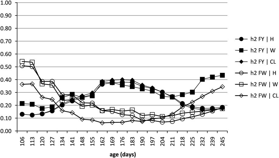
The h 2 estimates for FY were very similar between the models showing the same trend for higher values near 170 days of age. The only change in pattern was for FY with W after 211 days (Figure 5), but in general FY estimates ranged from 0.13 (113 days) to 0.40 for the interval from 162 to 183 days. On the other hand, h 2 estimates for FW were higher at the beginning of the studied period and presented a decreasing trend until the middle of the experimental period followed by a subsequent rise (Figure 5). The h 2 estimates for FW ranged from 0.08 (176 days) to 0.58 (245 days). Moreover, the differences in the bivariate analyses for FW are higher at the beginning and the end of the experimental period, as was observed for the morphometric traits.
Heritability of fillet yield or fillet weight, as a function of age, estimated by a bivariate random regression model including height (h 2 FY | H or FW | H), width (h 2 FY | W or FW | W) and corrected length (h 2 FY | CL or FW | CL).

Genetic correlations and correlated response efficiencies
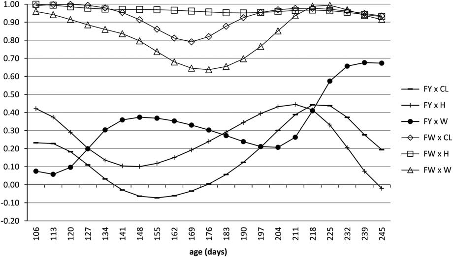
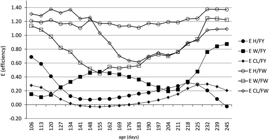
The genetic correlations between body measurements and FW (Figure 6) were generally strong and positive (most of the values between 0.8 and 1). The exceptions were the estimates with W, which presented a decreasing trend in the middle of the growth period reaching 0.64 around 176 days. The estimated CRE curves for FW when any morphometric trait was used as the selection criterion were also strong and positive (Figure 7), following a similar pattern of the genetic correlations. Estimated CRE values for FW ranged from 0.43 at 155 days with W, to 1.39 at 120 days with CL and at 239 days with H. Moreover, CRE curves for FW with W or CL were fairly similar presenting a decrement of CRE in the middle of studied ages. On the other hand, the curve for H was almost uniform across ages, with high values around 1.20. Therefore, the estimated CRE values are evidence of possible genetic gains for indirect selection of FW via selection for morphometric traits (especially H).
Genetic correlations of fillet yield or fillet weight with corrected length (FY×CL or FW×CL), height (FY×H or FW×H) and width (FY×W or FW×W) expressed from 106 to 245 days of age. Estimates were obtained from a bivariate random regression model including a random family effect and residual heterogeneity of variance.

Correlated response efficiency (E=r xy . i x . i y −1 . h x . h y −1) expressed from 106 to 245 days of age when the target trait was fillet yield or fillet weight and direct selection was for height (H/FY or H/FW), width (W/FY or W/FW) or corrected length (CL/FY or CL/FW). Selection intensity (i) was 2.27 (3%) for body measurements and 1.98 (6%) for FY or FW.

The genetic correlations between FY and morphometric traits (Figure 6) were, in general, lower than between FW and morphometric traits. The estimated values ranging from low negative with CL, around 155 days (−0.08), to high positive with W, around 239 days (0.68). It is worth note, that estimated genetic correlation curves with H and CL presented similar trends, but the estimates with H were higher for most of the period. On the other hand, the estimated genetic correlations with W presented an opposite behavior, with increasing trend when the correlations with H and CL are decreasing. As like for FW, the CRE curves for FY presented similar trend as the genetic correlation curves. Estimated values ranged from near 0 and negative from 134 to 183 days with CL to above 0.8 with W after 232 days. Therefore, despite the CRE for indirect selection of FY via morphometric traits be positive for most of the studied period the estimates never were above 1.
Discussion
Model selection
Results in Table 1 show the importance of considering the heterogeneity of residual variance in a longitudinal study. The inclusion of heterogeneity of variance is not only because it captures environmental changes, but for growth traits, it will also capture changes in scale and increase of total variance that appears as fish get old. The assumption of different classes of residual variance model better the increase of total variance, avoiding a possible spurious increase in h 2 estimations. The importance of family effect is shown in the Supplementary Table S2 and is in accordance with results reported in the literature (Rutten et al., Reference Rutten, Bovenhuis and Komen2005a; Turra et al., Reference Turra, Oliveira, Valente, Teixeira, Prado, Melo, Fernandes, Alvarenga and Silva2012b). The differences related to the selected number of classes of residual variance modeled for the analysis of FY with H or CL may be due to the fact that the structure for the genetic and residual variances for those traits across the studied period has fewer inflection points. This was shown for FY in a previous work from Turra et al. (Reference Turra, Oliveira, Valente, Teixeira, Prado, Melo, Fernandes, Alvarenga and Silva2012b). Therefore, the increase of classes of residual variance was not as advantageous for FY with H or CL as it was for the other bivariate analyses.
Interpretation of results from selected models
Attempting to infer important information from several traits at the same time is a difficult task. A glance at the literature about multiple trait models reveal several approaches, none been unanimously accepted as the best for every case. But, there is a consensus that joint estimation of genetic parameters of several traits can lead to increase in accuracy (Mrode and Thompson, Reference Mrode and Thompson2005; Schaeffer, Reference Schaeffer2016). An accepted and powerful approach for longitudinal data is to use multiple trait random regression, which was used in the case of the present study as bivariate random regression. The several bivariate models approach may lead to different results estimated from each of the models used. Despite the existence of methods for multi-model analysis and averaging (Burnham and Anderson, Reference Burnham and Anderson2004), the decision of presenting the results from different models was with the intention to show the reader the behavior of the selected models.
An interesting pattern that arose from the analysis of H, CL and W was that, for the ages that h 2 estimates were highest, differences between the estimates from selected models were also largest. That pattern may be due to two different facts: First, there are differences between the joint estimations of FW or FY with the morphometric traits. Those differences are due to the fact that several bivariate models were used which do not take into account the possible interactions between the morphometric. Thus, the estimated covariance matrix of the morphometric traits with FW can present differences from the one with FY and consequently estimated h 2 also can be different between models. Second, in the initial and final periods of growth, the density of data points was lower and may cause the random regression estimates to become less precise due to noise from sampling. It is plausible to assume that both phenomena occur, thus affecting the final results observed. Therefore, a more parsimonious inference about the h 2 results across ages for H, CL, and W is that the h 2 is probably intermediate to the values estimated by the different models.
Estimates of h 2 for fillet traits were in the same range of results from other studies. Rutten et al. (Reference Rutten, Komen and Bovenhuis2005b) presented h 2 of 0.24 and 0.12 for FW and FY respectively, while Nguyen et al. (Reference Nguyen, Ponzoni, Abu-Bakar, Hamzah, Khaw and Yee2010) reported h 2 of 0.33 and 0.25 for FW and FY, respectively, and Turra et al. (Reference Turra, Oliveira, Valente, Teixeira, Prado, Melo, Fernandes, Alvarenga and Silva2012b) reported maximum h 2 of 0.25 and 0.40 around 175 days for FW and FY, respectively. Only Turra et al. (Reference Turra, Oliveira, Valente, Teixeira, Prado, Melo, Fernandes, Alvarenga and Silva2012b) reported estimates of h 2 for fillet traits in the same range of ages but using univariate random regression. The h 2 estimates show in the current work for FY presented similar curve as the univariate reported before. But, for FW the curves presented here differs from the one estimated via univariate random regression previously. In the current work, the highest estimates of h 2 for FW is at the limits of the studied age interval, whereas previously the trajectory of h 2 for FW was similar to the trajectory for FY. These differences between estimates from bivariate and univariate analyses are probably due to the joint estimate of covariance with the morphometric traits. One of the characteristics of multiple trait approaches is that the estimated parameters for each trait will be influenced by the correlations between traits. Therefore, the differences between bivariate analyses were expected as each morphometric trait showed different h 2 curves and correlations with FY and FW. The estimates of genetic correlations between morphometric traits and FY (Figure 6) were lower than for FW and therefore had less influence on the estimates of h 2 for the bivariate analysis between FY and the morphometric traits. On the other hand, the high genetic correlations of FW with morphometric traits shows how much FW is more related to morphometric traits. This is also supported by the fact that the estimated curves for h 2 of FW and of the morphometric traits presented similar trends.
The CRE estimates presented here show that appreciable gains may be achieved for FW if selection were performed on morphometric traits, primarily H and CL (as CL showed advantageous estimates before 162 days of age). It is worth of note that with RRM it is possible to estimate genetic correlations between traits measured at different time points (e.g. genetic correlation between FW measured at 240 days and CL at 20 days). This is powerful for a CRE analysis, however, in the present study higher genetic correlations were estimated for traits at the same age, thus values for CRE of traits in different ages were omitted as they were lower than their counterpart for the traits measured at the same age. These results are perhaps more interesting than using BW as a selection criterion (Turra et al., Reference Turra, Oliveira, Valente, Teixeira, Prado, Melo, Fernandes, Alvarenga and Silva2012b). Therefore, it is safe to say that these traits are an effective alternative for tilapia breeding programs focused on improving FW. In addition to this, no appreciable losses in BW would be expected due to the high genetic correlation between BW and morphometric traits and FW (Rutten et al., Reference Rutten, Bovenhuis and Komen2005a; Fernandes et al., Reference Fernandes, Silva, Alvarenga, Teixeira, Silva, Alves, Salles, Manduca and Turra2015).
Given the importance of FY, there are few studies that tried to investigate its genetic parameters and genetic correlations with BW or other measurements in tilapia (Rutten et al., Reference Rutten, Bovenhuis and Komen2005a; Nguyen et al., Reference Nguyen, Ponzoni, Abu-Bakar, Hamzah, Khaw and Yee2010; Turra et al., Reference Turra, Oliveira, Valente, Teixeira, Prado, Melo, Fernandes, Alvarenga and Silva2012b). However, their results vary, ranging from moderate to high positive values. Note that, the high positive values for correlation is with carcass yield, another trait that can be measured only via the sacrifice of the fish. The results presented here also were unsatisfactory in find a correlated trait for selection of FY. Therefore, the results of CRE for morphometric traits as an indirect selection criterion for FY (Figure 7) were in general positive, but with values always below 1.0 and behave similarly to the curves of their respective genetic correlations. Those results indicated low to moderate improvement in FY would be expected if morphometric traits were used as the selection criteria. Thus, as FY is in general positively correlated with body measurements, the current selection on BW used by many breeding programs is probably leading to some gains in FY as well. However, in order for a breeding program decides if it is interesting to include FY as an objective of selection several factors must be addressed. First, the economic value of FY for a breeding program must be estimated, and that will vary depending on the target market and objectives of each breeding program. This economic value will be important in order to define selection strategies. Second, it is important to note that the CRE values estimated here were for abstract selection intensities of 3% for body measurements and 6% for fillet traits. Those values were chosen based on a selection scheme for fillet traits were half of the candidate from each family must be slaughtered in order to estimate breeding values for the remaining fish. But, the possible selection intensities may differ on a real breeding program, and that also will dictate if it is more interesting to do the direct or indirect selection for fillet traits. At last, despite the trend for positive CRE for FY, there is no empirical evidence regarding an actual response in FY when selecting fish for morphometric traits or BW. As FY is a trait difficult to measure, there is probably a high level of noise masking the estimates of its genetic parameters. Therefore, it is important to continue the search for another measure of FY production.
Conclusion
In conclusion, the use of morphometric traits as selection criteria can lead to high indirect gains in FW with moderate gains in FY. Therefore, the inclusion of H, W and CL as a selection criterion of Nile tilapia breeding programs is interesting in order to attain higher gains for FW and moderate for FY. Also, this increase in gains for FW and FY is without prejudice for BW as those morphometric traits have a strong and positive genetic correlation with BW. Moreover, H was the trait that shows a steadier CRE for FW with values above 1 through the whole studied period. But, optimal indirect gains for FW and FY may be realized if selection were done near 240 days of age. However, the question of the use of morphometric traits in selection needs more investigation, mainly in the area of economic efficiency. Therefore, factors as, the increased costs of labor needed to measure several traits and the economic gains of producing fish with heavier fillets and higher yield need to be addressed in future research in order to address the decision of including other traits in the selection.
Acknowledgments
This research received support from Conselho Nacional de Desenvolvimento Científico e Tecnológico (CNPq, Brazil – 472081/2012-8 and 472149/2012-1) and Pró-Reitoria de Pesquisa da Universidade Federal de Minas Gerais (PRPQ-UFMG, Brazil).
Supplementary Material
To view supplementary material for this article, please visit https://doi.org/10.1017/S1751731117001768