1 Introduction
Researchers of political psychology, intergroup prejudice, media effects, learning, public health, and more frequently test how randomized stimuli affect outcomes measured in surveys. For example, experiments that measure the effects of randomized stimuli presented in a survey on individuals’ responses to questions in the same survey (“survey experiments”) constitute a dominant paradigm in political science (Sniderman and Grob Reference Sniderman and Grob1996; Druckman et al. Reference Druckman, Green, Kuklinski and Lupia2006); leading political science journals publish dozens of survey experiments each year (Hainmueller, Hopkins, and Yamamoto Reference Hainmueller, Hopkins and Yamamoto2014, p. 1).
Along with political scientists’ strong interests in survey research and experiments, there has been increasing interest in field experiments with survey outcomes: experiments where outcomes are measured by surveys but randomized stimuli are delivered by a separate mechanism in the real world, such as by mailers, door-to-door canvasses, phone calls, or online ads. Unfortunately, low rates of survey response and treatment compliance in many countries mean common designs for such experiments present scholars several barriers. First, common designs for such experiments are often infeasibly expensive. For example, an experiment well-powered to detect a “small” treatment effect of 0.1 standard deviations on a survey outcome could cost under  as a survey experiment using Mechanical Turk but easily over
 as a field experiment using designs common today (see next section). In addition, the results of such experiments are vulnerable to bias from differential attrition, which occurs when treatments influence survey completion. This has been shown to occur and produce meaningfully large bias, yet is often undetectable with common designs (Bailey, Hopkins, and Rogers Reference Bailey, Hopkins and Rogers2016). Finally, to be well-powered they require real-world intervention on a grand scale, raising ethical concern (Michelson Reference Michelson2016).
This paper makes three related contributions that can help researchers conduct field experiments with survey outcomes that are significantly more feasible, precise, robust, and ethical.
Our first contribution is to describe and analytically decompose previously undocumented complementarities between four methodological practices currently uncommon in such experiments. These are: (1) surveys administered online to a sample recruited from an ex ante defined sampling frame (e.g., Barber et al. Reference Barber, Mann, Quin Monson and Patterson2014), (2) with at least one baseline wave prior to treatment (Iyengar and Vavreck Reference Iyengar and Vavreck2012) (3) with multiple measures of outcomes gathered and combined into an index at each wave (Ansolabehere, Rodden, and Snyder Reference Ansolabehere, Rodden and Snyder2008) and, if possible, (4) a placebo wherein control subjects are contacted with an unrelated appeal (Nickerson Reference Nickerson2005b).
The complementarities between these four practices have not been previously documented to our knowledge yet can yield extremely large gains. These practices are not novel on their own. Moreover, in common cases, when used alone each one does not increase efficiency considerably or at all. However, these practices interact in a nonadditive way such that employing at least two in combination can dramatically relax the constraints typically associated with field experiments with survey outcomes; in some examples, they decrease variable costsFootnote 1 by 98%.
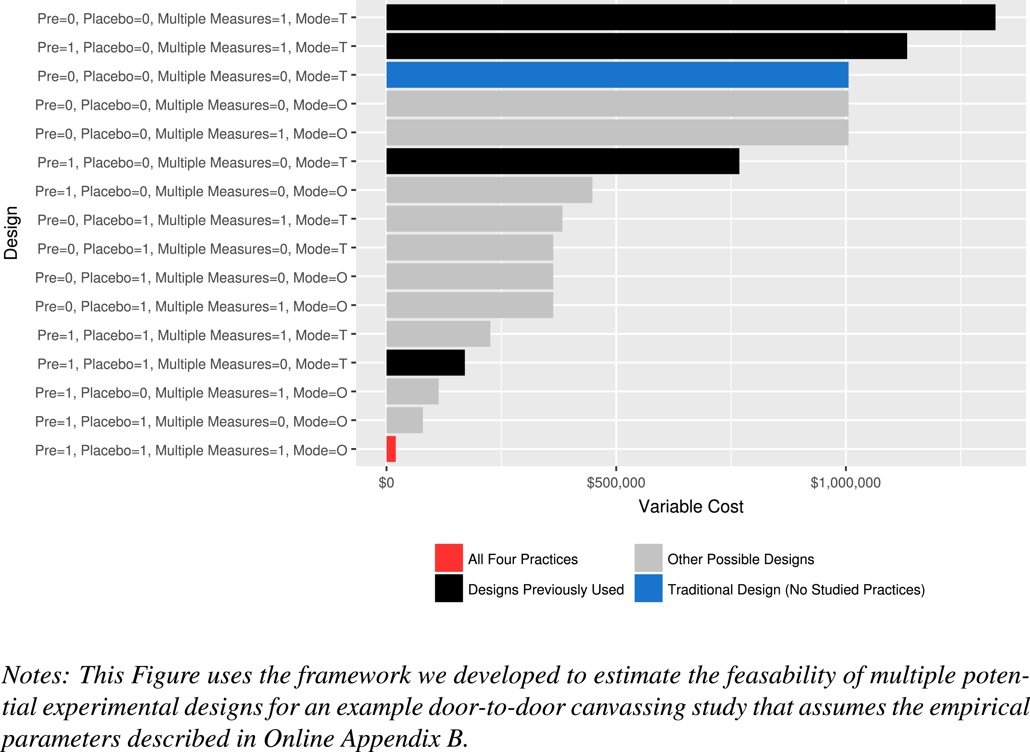
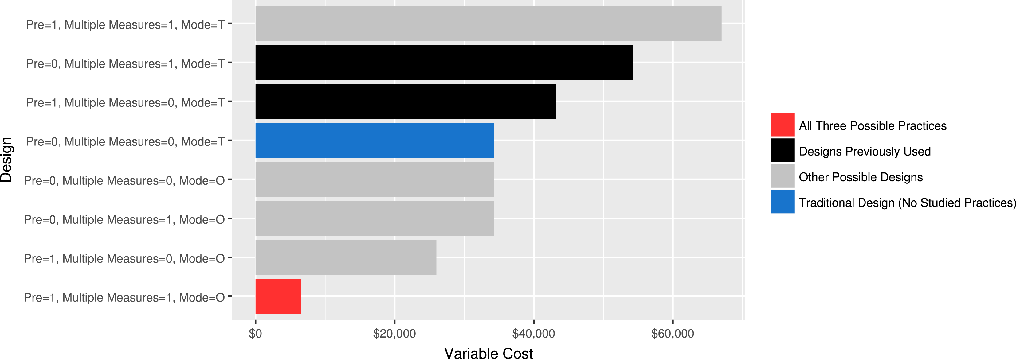
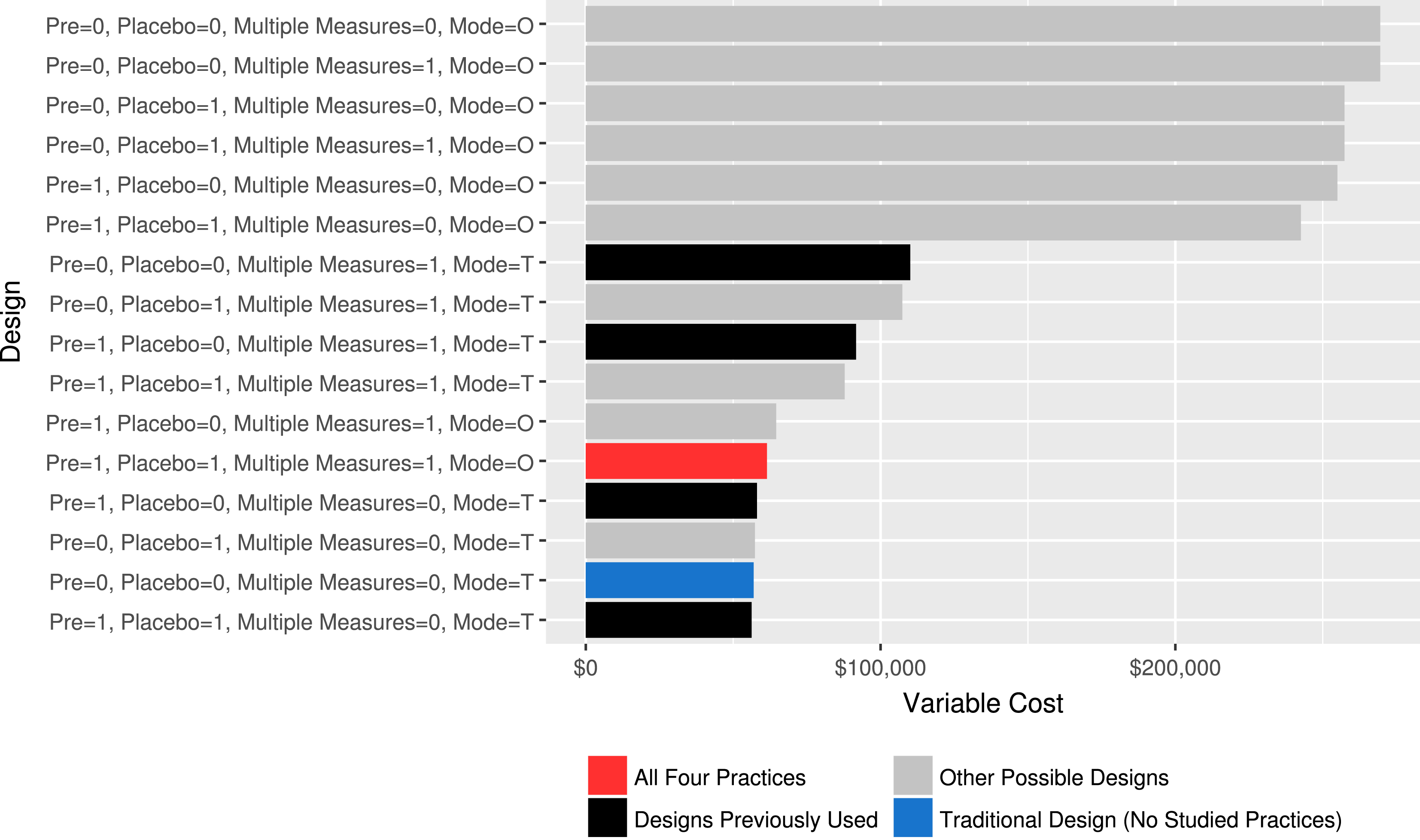
Figure 1 previews some of our results about how these practices can interact in common settings. The figure considers the variable costs of conducting a study in a common setting in the literature, an experiment studying the persuasive effect of door-to-door canvassing of registered voters in the United States that measures outcomes in two rounds of posttreatment surveys, to measure both short-run and long-run effects. Each row in Figure 1 corresponds to a different possible design, all sixteen permutations of using or not using each of the four practices we study. The length of each bar corresponds to the cost of each possible design for achieving a fixed level of precision (a standard error of 0.045 standard deviations), assuming empirical parameters about survey costs and so forth estimated from two empirical studies.Footnote 2 The blue bar shows the variable costs of a traditional experiment employing the modal design in the literature, which employs none of the four practices we study and relies on a telephone survey (denoted T) instead of an online survey (denoted O) to collect outcomes. The black bars show costs for other designs from existing literature, which have employed some of these practices but rarely multiple in combination. The gray bars show other permutations of designs that might be possible if one were to employ different subsets of these practices. Finally, the red bar shows the variable cost of an experiment using all four practices.
Figure 1 shows that, in this common setting, an experiment using all four practices can be significantly more feasible than an experiment using only one of these practices. An experiment with a variable cost of over  with none of these practices could instead cost approximately
 In addition, such an experiment would be able to precisely test additional design assumptions and require real-world intervention on only a minuscule scale.
Comparing feasibility of different designs.

Of course, Figure 1’s empirical results about the benefits of these four practices are specific to a particular intervention, population, and context. Accordingly, this paper’s second contribution is a general and extensible framework that allows researchers to select the most efficient mix of these practices in a wide variety of applications and that can be easily extended to accommodate unique features of particular settings. This framework analytically captures the effect of parameters such as survey response rates, treatment application rates, and the stability of survey responses on the cost of field experiments with survey outcomes that do or do not employ each of the four practices we consider. This framework also captures the gains in efficiency that can arise from the complementarities between the four practices we study. We provide several examples of how researchers can use this framework to select more efficient, robust, and ethical designs in a wide variety of applications, just as Figure 1 did for US door-to-door canvassing study.
Our third contribution is new empirical studies that examine how these practices perform in practice. A first empirical study examines the representativeness of the samples that can be recruited with the survey mode we study: online surveys recruited from a defined sampling frame and surveyed online at least twice. This first study recruited a sample in this manner and compared it to a common approach. In particular, we recruited US registered voters to two rounds of online surveys by mail and compared this sample’s representativeness to a sample of the same recruited by the traditional means in existing literature, telephone. Although different recruitment methods may yield different results in different settings, results of this study suggest this recruitment strategy compares favorably to common practice. A second empirical study successfully deploys all four practices in the context of an original field experiment measuring the effects of a door-to-door canvassing effort targeting abortion attitudes. This study estimated a precise (null) effect, indicating it is practical to implement all four of these practices together and that doing so appears able to evade a variety of potential biases.
We conclude by discussing remaining limitations and potential extensions.
2 Field Experiments With Survey Outcomes: Typical Designs And Their Challenges
2.1 Designs common in the literature
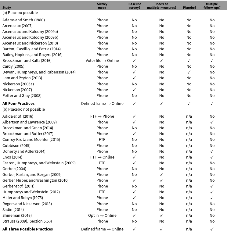
How do political science researchers typically conduct field experiments with survey outcomes today? Table 1 catalogs the existing, publicly available political science field experiments with survey outcomes of which we are aware.
Existing political science field experiments with survey outcomes.

Table 1 establishes the novelty of this paper’s first contribution, which notes the complementarities between the four practices we study. In particular, the table shows that existing experiments rarely take advantage of the complementarities between these practices. These practices are: (1) surveys administered online to a sample recruited from a list sampling frame of the target population units (Cheung Reference Cheung2005, e.g., a public list of registered voters, a civil registry, membership lists of an activist group, etc.), (2) with at least one baseline wave prior to treatment, (3) with multiple measures of outcomes gathered at each wave analyzed as an index and, if possible, (4) a placebo control. The middle four columns in Table 1 record whether each existing study uses each of these practices. They show that each of these individual practices only occasionally appears in field experiments with survey outcomes. Moreover, these design features rarely appear together in the same field experiment, except in one study we have conducted using this paper’s ideas (Broockman and Kalla Reference Broockman and Kalla2016).
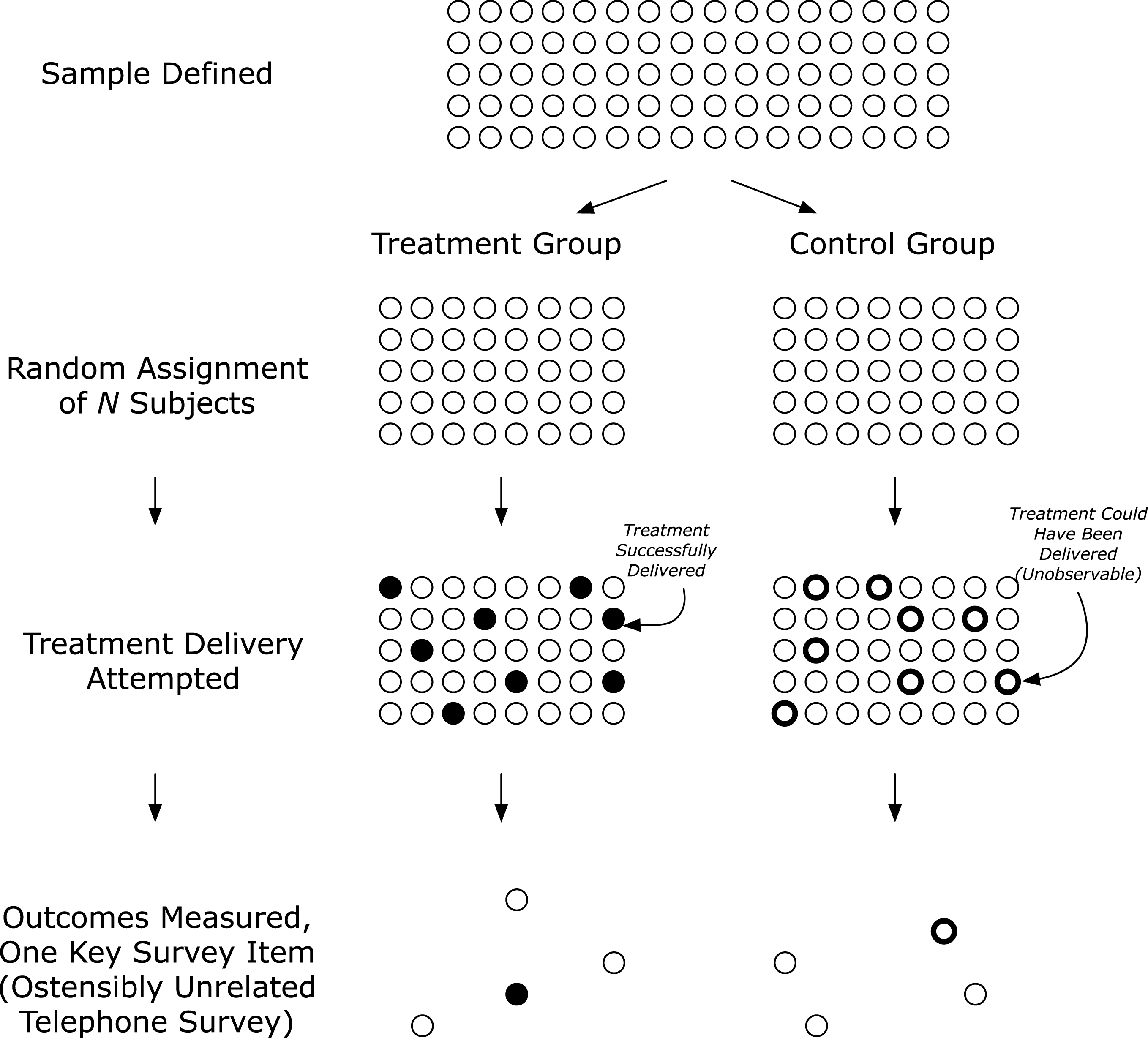
To build familiarity with existing practice, Figure 2 depicts the modal design of the field experiments in Table 1a. Such experiments could employ all of the four practices we study but employ none of them. We call this “the traditional design.” An analyst first defines a sample of individuals and randomly assigns them to treatment and control groups. Delivery of the treatment is attempted to treatment group subjects, but many treatment group subjects are not successfully treated. Control group subjects are not contacted. All subjects originally assigned to either condition are then solicited for an ostensibly unrelated follow-up survey, which few answer, that contains one key survey item of interest.
“The Traditional Design.”

2.2 Challenges field experiments with survey outcomes often face
In this section we review challenges field experiments with traditional designs often face. The following section will formalize how the methodological practices we describe can ameliorate each, especially when used in combination.
To help illustrate key ideas, throughout we assume several example values for marginal costs of surveys, treatment, etc. Online Appendix B describes how we calculated these example values from our empirical studies and the literature. However, we caution readers that these example values are for exposition purposes only and likely vary across contexts and time.
2.2.1 Failure to treat
Failure to treat arises when some treatment group subjects are not successfully administered treatment. It increases necessary sample sizes (Gerber and Green Reference Gerber and Green2012). To appreciate how, imagine planning an experiment to assess the impact of a door-to-door canvassing treatment powered to detect a 5 percentage point effect. Further suppose canvassers contact 20% of treatment group subjects (as in Bailey, Hopkins, and Rogers Reference Bailey, Hopkins and Rogers2016). A 5 percentage point effect among those contacted would manifest as an overall difference of
 $5\times 0.20=1$
percentage point between the entire treatment and control groups. A final sample of approximately 80,000 survey responses would be required to detect this 1 percentage point effect with 80% power.
The budgetary implications of failure to treat are especially unfavorable in field experiments with survey outcomes because it increases both the number of subjects one must treat and the number of subjects one must survey. Consider the example just discussed hoping to yield 80,000 survey responses for analysis. Assuming for the moment that survey response rates are 100%, the experimenter must pay to knock on the doors of the 40,000 subjects in the treatment group and to survey all 80,000 subjects. At marginal costs of  per canvass attempt and
 per survey response, the experiment’s variable cost would be
 of which
 is survey costs. However, if all subjects in the treatment group could be actually treated, only 3,200 subjects would be necessary, resulting in variables costs of only
 with only
 in survey costs.
2.2.2 Survey nonresponse
Field experiments with survey outcomes usually collect outcomes by telephone, and response rates to telephone surveys in the United States and other developed countries are now typically under 10% (Kohut et al.
Reference Kohut, Keeter, Doherty, Dimock and Christian2012). In anticipation of this nonresponse, analysts must treat many more subjects, increasing treatment costs. To see how, consider the experiment described above. Anticipating a response rate of 10% to a final survey, an analyst must attempt to canvass 400,000 voters in order to yield 40,000 voters both attempted for canvassing and then successfully surveyed. Assuming marginal treatment costs scale linearly, this would increase treatment variable costs from  to
 (in addition to the
 in survey costs already discussed).
2.2.3 Limited pretreatment covariates available
Finally, many field experiments with survey outcomes have few pretreatment covariates available that predict outcomes well. For example, Bailey, Hopkins, and Rogers (Reference Bailey, Hopkins and Rogers2016) found that commercial scores and administrative data could only predict survey responses to a presidential vote choice question with an
 $R^{2}$
of 0.005. Such limited predictive power has several disadvantages. First, although baseline covariates can increase the precision of estimates (e.g., Sävje, Higgins, and Sekhon Reference Sävje, Higgins and Sekhon2016), covariates that predict outcomes poorly do not meaningfully do so. For example, when
 $R^{2}=0.005$
, the sample size necessary to achieve the same precision decreases by only 0.5%. In addition, lacking prognostic covariates makes differential attrition difficult to detect. Differential attrition arises when the treatment influences survey response rates,Footnote
3
leading the surveyed treatment and control groups to differ in expectation even if the treatment has no effect (Gerber and Green Reference Gerber and Green2012, chap. 7). Any experiment with survey outcomes without prognostic pretreatment covariates cannot persuasively evaluate the assumption of no differential attrition, even though this assumption has been found to fail (Bailey, Hopkins, and Rogers Reference Bailey, Hopkins and Rogers2016). Finally, the absence of pretreatment covariates also precludes testing many theories with predictions about how treatment effects are moderated by prior attitudes or previous exposure (e.g., Druckman and Leeper Reference Druckman and Leeper2012).
3 Deriving A Framework for Selecting Experimental Designs
The practices we study are able to substantially ameliorate many of these challenges. In this section we provide a formal analysis comparing the asymptotic efficiency of experiments that employ some or all of the practices we consider to the traditional design shown in Figure 2. We first describe and consider the trade-offs each of these practices involves and how each practice complements the others. We then use these analyses to build a framework for evaluating trade-offs between possible designs using different mixes of these four practices.
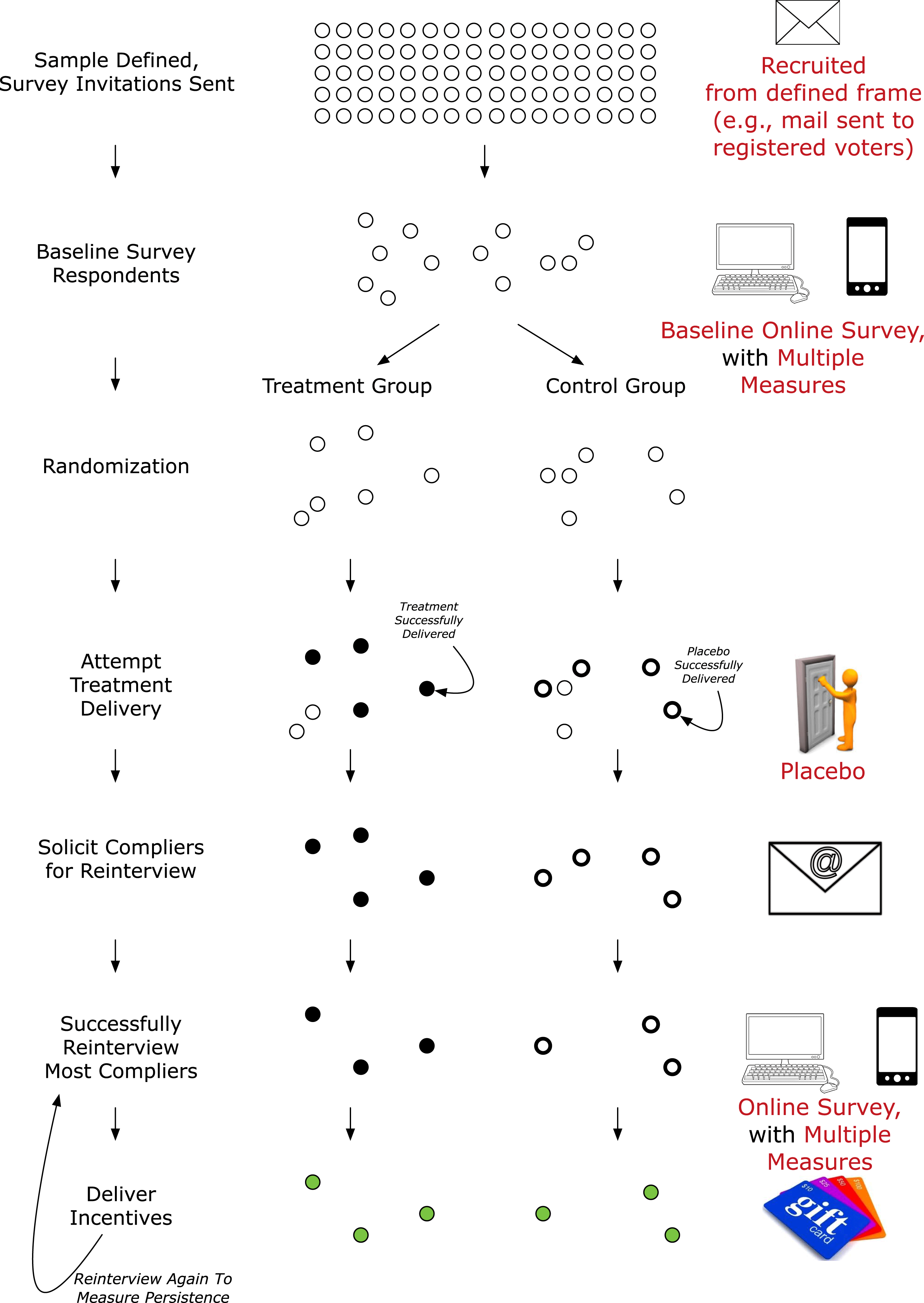
Our framework can accommodate a wide variety of possible settings, and all four of the practices we study will not be optimal in all these settings. However, to build understanding about how each of these practices logistically functions, we begin by describing a possible study using all four practices in the setting of a door-to-door canvassing experiment targeting US registered voters’ attitudes, just like many existing studies reported in Table 1a and our application study. First, a researcher would send mail to a sampling frame of registered voters inviting them to complete a baseline online survey with multiple measures of outcomes. The survey collects respondents’ email addresses so that they can be invited to follow-up surveys later. Next, treatment is delivered to baseline survey respondents only, as is a placebo if possible. Only respondents to the baseline survey are targeted with a real-world intervention ostensibly unrelated to the survey. For example, a canvasser may visit baseline survey respondents’ homes and deliver either the treatment or placebo. Finally, the researcher conducts a follow-up survey, but only of individuals who were contacted. Respondents are invited via email to complete these follow-up surveys. Appendix Figure 11 depicts this example design, with the practices we study noted in red.
3.1 Setup for formal analysis
In this subsection, we detail the assumptions and estimators that form the basis of our formal analysis of the four practices we study. Readers familiar with the design and analysis of experiments with noncompliance may wish to skip this subsection.
We assume a random sample of size
 $N$
from an infinite population. Let
 $z_{i}\in \{0,1\}$
denote the treatment randomly assigned to subject
 $i$
, and let
 $d_{i}(z)\in \{0,1\}$
indicate whether subject
 $i$
is actually treated when the treatment assignment
 $z_{i}=z$
. Let
 $Y_{i}(z,d)$
denote the potential outcome for subject
 $i$
when
 $z_{i}=z$
and
 $d_{i}=d$
. We assume the usual noninterference assumption, so the potential outcome of
 $i$
only depends on the treatment subject
 $i$
is assigned. We also make the usual exclusion assumption,
 $Y_{i}(z,d)=Y_{i}(d)$
. We define
 $Y_{i}(z=1)=Y_{i}(z=1,d=d_{i}(1))$
. Compliers are those subjects who take treatment when they are assigned to the treatment group, and do not take treatment when they are assigned to the control group—i.e., subjects for whom
 $d_{i}(1)=1$
and
 $d_{i}(0)=0$
. We assume no subjects assigned to control are treated, such that
 $d_{i}(0)=0$
for all
 $i$
.
Our estimand of interest is the Complier Average Causal Effect (Gerber and Green Reference Gerber and Green2012, p. 142) defined as:
 $$\begin{eqnarray}\displaystyle & \text{CACE}=\mathbb{E}[Y_{i}(d=1)-Y_{i}(d=0)\mid d_{i}(0)=0,d_{i}(1)=1]. & \displaystyle\end{eqnarray}$$
An alternative estimand, which ignores compliance, is the intent-to-treat estimand defined as:
 $$\begin{eqnarray}\displaystyle \text{ITT} & = & \displaystyle \mathbb{E}[Y_{i}(z=1)-Y_{i}(z=0)]\nonumber\\ \displaystyle & = & \displaystyle \mathbb{E}[Y_{i}(z=1,d(1))-Y_{i}(z=0,d(0))].\nonumber\end{eqnarray}$$
The intent-to-treat effect of treatment assignment (
 $z$
) on compliance (
 $d$
) is defined as:
 $$\begin{eqnarray}\displaystyle & \text{ITT}_{d}=\mathbb{E}[d_{i}(1)-d_{i}(0)], & \displaystyle \nonumber\end{eqnarray}$$
which equals
 $\mathbb{E}[d_{i}(1)]$
because
 $d_{i}(0)=0$
for every
 $i$
with one-way noncompliance.
With this setup, CACE can be estimated in two ways. First, we can observe who in the control group could have been treated with the placebo design (Nickerson Reference Nickerson2005b). Observing
 $d(1)$
for all
 $i$
, we can plug in sample estimates in Equation (1). We refer to this estimator as
 $\widehat{\text{CACE}}_{\text{Placebo}}$
.
The second approach, more common in existing field experiments with survey outcomes and noncompliance, is:
 $$\begin{eqnarray}\displaystyle & \displaystyle \widehat{\text{CACE}}_{\text{ITT}}={\displaystyle \frac{\text{ITT}}{\text{ITT}_{d}}}, & \displaystyle \nonumber\end{eqnarray}$$
which motivates the usual instrumental variables estimator. As with all field experiments with survey outcomes and noncompliance, both estimates are local to compliers who complete surveys (an issue we return to below).
One may use the delta method to obtain the following asymptotic variance for
 $\widehat{\text{CACE}}_{\text{ITT}}$
:
 $$\begin{eqnarray}\displaystyle & \displaystyle \mathbb{V}(\widehat{\text{CACE}}_{\text{ITT}})={\displaystyle \frac{1}{\text{ITT}_{d}^{2}}}\mathbb{V}(\widehat{\text{ITT}})+{\displaystyle \frac{\text{ITT}^{2}}{\text{ITT}_{d}^{4}}}\mathbb{V}(\widehat{\text{ITT}}_{d})-2{\displaystyle \frac{\text{ITT}}{\text{ITT}_{d}^{3}}}\mathbb{C}(\widehat{\text{ITT}},\widehat{\text{ITT}}_{d}), & \displaystyle\end{eqnarray}$$
where
 $\mathbb{C}$
denotes covariance.
Prior work in this literature has examined the asymptotic variance of estimators of
 $\widehat{\text{CACE}}_{\text{ITT}}$
assuming that the estimate of
 $\text{ITT}_{d}$
is fixed and hence ignoring the last two terms of Equation (2) (Nickerson Reference Nickerson2005b; Gerber and Green Reference Gerber and Green2012):
 $$\begin{eqnarray}\displaystyle & \displaystyle \mathbb{V}(\widehat{\text{CACE}}_{\text{ITT}})\approx {\displaystyle \frac{1}{\text{ITT}_{d}^{2}}}\mathbb{V}(\widehat{\text{ITT}}). & \displaystyle\end{eqnarray}$$
For our purposes, ignoring the last two terms in Equation (2) allows for a cleaner comparison between the variance of
 $\widehat{\text{CACE}}_{\text{ITT}}$
and the variance of
 $\widehat{\text{CACE}}_{\text{Placebo}}$
. As previous authors have noted, these last two terms make little difference in practice. Indeed, the variance of traditional experiments relying on
 $\widehat{\text{CACE}}_{\text{ITT}}$
is often actually slightly larger than given in Equation (3), making our comparative statements about the efficiency of
 $\widehat{\text{CACE}}_{\text{Placebo}}$
more conservative.Footnote
4
We also make several additional assumptions throughout to simplify exposition of the key ideas. We assume a balanced experimental design with 50% allocation to treatment and 50% allocation to control. We further assume that there is a constant treatment effect, and hence that the true variance of the potential outcomes in the subject pool is the same for treated and control subjects (
 $\mathbb{V}[Y(0)]=\mathbb{V}[Y(1)]=\unicode[STIX]{x1D70E}^{2}$
). For simplicity, this variance is assumed to be 1.
Given these simplifications:
 $$\begin{eqnarray}\mathbb{V}(\widehat{\text{CACE}}_{\text{ITT}})\approx \frac{4\unicode[STIX]{x1D70E}^{2}}{\mathit{NA}^{2}},\end{eqnarray}$$
where
 $N$
is the number of subjects randomly assigned, and
 $A$
is the application or contact rate (
 $\text{ITT}_{d}$
).
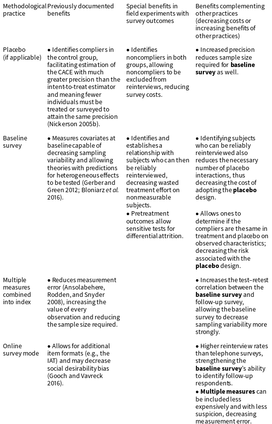
Potential benefits of and complementarities between four methodological practices.

3.2 How the four practices can increase efficiency
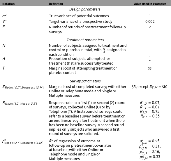
We next formally analyze how each of the four practices we discuss can increase efficiency individually and together. Table 2 verbally summarizes our points. It discusses the primary advantages of each of these practices as it has previously been understood, our results about the special benefits each practice can have in field experiments with survey outcomes, and our results about how each practice can complement others in field experiments with survey outcomes to yield additional improvements.
For our formal analysis of how each of these four practices can increase efficiency, we consider how an experiment’s variable costs
 $c_{P,B}(\cdot )$
vary with different design choices.
 $P\in \{0,1\}$
indicates whether the placebo is used and
 $B\in \{0,1\}$
indicates whether a baseline survey is used. Variable cost
 $c(\cdot )$
is a function of many variables. To reduce notational clutter, we exclude irrelevant variables in each instance and let the context dictate the parametrization. We focus on how variable cost varies as a function of the required sample size
 $N$
or a desired variance
 $V^{\ast }$
, the number of rounds of posttreatment follow-up surveys one wishes to conduct
 $F$
(e.g., for
 $F=2$
if one wants to test both whether there is an initial treatment effect and then whether any effect lasts in a subsequent round of surveying), and when considered, the marginal cost of attempting treatment
 $T$
and conducting a survey
 $S$
.
Note that these parameters are examples only and could vary dramatically in different settings. See Online Appendix Section B for details on how we calculated these example parameter values. Moreover, note that we consider variable costs only, and do not take into account fixed costs such as purchasing voter lists, training canvassers, renting office space, or traveling to a country to conduct an experiment.
Table 3 will keep track of notation and the parameter values from our empirical studies we use in our examples.
Notation and values used in examples.

3.2.1 Practice 1: Placebo
If failure to treat can occur and be observed, a placebo condition can increase efficiency dramatically (Nickerson Reference Nickerson2005b). In an experiment with a placebo condition, subjects in the control group are contacted with an unrelated appeal. The purpose of these placebo contacts is to identify control subjects to whom treatment could be delivered—that is, to identify whether control group subjects are compliers or noncompliers. For example, in our second empirical study, canvassers contacted individuals in placebo households about recycling.Footnote 5 Subjects in each group who open the door and identify themselves before either regime begins are then used at the basis for comparison when estimating the CACE.
The variance of the CACE estimator with the placebo design is:
 $$\begin{eqnarray}\mathbb{V}(\widehat{\text{CACE}}_{\text{Placebo}})=\frac{4\unicode[STIX]{x1D70E}^{2}}{\mathit{NA}},\end{eqnarray}$$
where
 $A$
is the fraction of the
 $N$
subjects who are contacted, such that
 $\mathit{NA}$
is the number of contacted subjects whose outcomes are compared during estimation. As Nickerson (Reference Nickerson2005b) shows,
 $\widehat{\text{CACE}}_{\text{Placebo}}$
is unbiased under several assumptions: “(1) the [treatment and placebo] have identical compliance profiles; (2) the placebo does not affect the dependent variable; and (3) the same type of person drops out of the experiment for the two groups.”
As previously studied, the benefit of the placebo design is that it can reduce the number of subjects with whom contact must be attempted (Nickerson Reference Nickerson2005b). To see this advantage, let
 $T$
be the marginal cost of attempting to contact a subject to deliver the treatment or placebo (such as the price a paid canvassing firm charges or the opportunity cost of a graduate student’s time “per knock”). Considering only the cost of attempting to treat subjects, the cost of implementing the traditional design in a sample of size
 $N$
with no placebo and no baseline survey is
 $c_{P=0,B=0}(N,T)={\textstyle \frac{1}{2}}\mathit{NT}$
, as only the
 ${\textstyle \frac{1}{2}}N$
subjects in the treatment group are attempted to be contacted. Suppose an experiment is being planned with the aim of achieving an estimate with variance
 $V^{\ast }$
. Using Equation (4), delivering treatment in the traditional design thus costs
 $c_{P=0,B=0}(V^{\ast },T)\approx {\textstyle \frac{1}{2}}\ast 4({\textstyle \frac{\unicode[STIX]{x1D70E}^{2}}{V^{\ast }}})({\textstyle \frac{1}{A^{2}}})T=2({\textstyle \frac{\unicode[STIX]{x1D70E}^{2}}{V^{\ast }}})({\textstyle \frac{1}{A^{2}}})T$
. In the placebo design, control group subjects are attempted with the placebo contact. Contact is therefore attempted with all
 $N$
subjects, such that
 $c_{P=1,B=0}(N,T)=\mathit{NT}$
. Using Equation (5), delivering treatment in the placebo design costs
 $c_{P=1,B=0}(V^{\ast },T)=4({\textstyle \frac{\unicode[STIX]{x1D70E}^{2}}{V^{\ast }}})({\textstyle \frac{1}{A}})T$
. The placebo design is therefore cheaper when
 $4({\textstyle \frac{\unicode[STIX]{x1D70E}^{2}}{V^{\ast }}})({\textstyle \frac{1}{A}})T<2({\textstyle \frac{\unicode[STIX]{x1D70E}^{2}}{V^{\ast }}})({\textstyle \frac{1}{A^{2}}})T$
, which reduces to
 $A<{\textstyle \frac{1}{2}}$
(Nickerson Reference Nickerson2005b).
Less well-appreciated is that a placebo can produce even larger efficiency gains in field experiments with survey outcomes because noncompliers need not be surveyed. Without a placebo, all subjects must be surveyed. Incorporating the cost of surveying,
 $c_{P=0,B=0}(N,F,T,S)=N({\textstyle \frac{1}{2}}T+\mathit{FS})$
, where
 $F$
is the number of rounds of posttreatment follow-up surveys and
 $S$
is the marginal cost of a survey, assuming a 100% survey response rate for now. To achieve an estimate with some desired variance
 $V^{\ast }$
, using Equation (4) reveals that the traditional design will cost
 $c_{P=0,B=0}(V^{\ast },F,T,S)\approx 4({\textstyle \frac{\unicode[STIX]{x1D70E}^{2}}{V^{\ast }}})({\textstyle \frac{1}{A^{2}}})({\textstyle \frac{1}{2}}T+\mathit{FS})$
. Supposing an example contact rate of
 $A=1/4$
,
 $c_{P=0,B=0}(V^{\ast },F,T,S)\approx ({\textstyle \frac{\unicode[STIX]{x1D70E}^{2}}{V^{\ast }}})(32T+64\mathit{FS})$
. However, with a placebo, “the group receiving the placebo can serve as the baseline for comparison for the treatment group” (Nickerson Reference Nickerson2005b). This means subjects who are not successfully contacted in the treatment or placebo groups—all noncompliers—do not need to be surveyed. This reduces survey costs. Incorporating the cost of surveying the
 $AN$
compliers only,
 $c_{P=1,B=0}(N,F,T,S)=N(T+FAS)$
. Using Equation (5), the placebo design will cost
 $c_{P=1,B=0}(V^{\ast },F,T,S)=4({\textstyle \frac{\unicode[STIX]{x1D70E}^{2}}{V^{\ast }}})({\textstyle \frac{1}{A}})(T+FAS)$
. Again supposing
 $A=1/4$
, this reduces to
 $c_{P=1,B=0}(V^{\ast },F,T,S)=({\textstyle \frac{\unicode[STIX]{x1D70E}^{2}}{V^{\ast }}})(16T+4\mathit{FS})$
. Note that with
 $A=1/4$
the placebo reduces the costs associated with delivering treatment by half (
 $32T$
to
 $16T$
) but reduces survey costs 16-fold (
 $64\mathit{FS}$
to
 $4\mathit{FS}$
). With
 $F=2$
,
 $T=3$
, and
 $S=5$
, this is equivalent to an 88% decrease in variable costs.
Illustrating the first way the practices we study can complement each other, a placebo also reduces the costs of baseline surveys by reducing the number of subjects who must be recruited to a pretreatment baseline if one is used. To see this, suppose a baseline survey of
 $N$
subjects is conducted before treatment. Let the marginal cost of each baseline survey also be
 $S$
. The baseline’s variable costs thus are
 $\mathit{NS}$
. The gross variable cost of incorporating a baseline is an increase in costs of
 $4({\textstyle \frac{\unicode[STIX]{x1D70E}^{2}}{V^{\ast }}})({\textstyle \frac{1}{A^{2}}})S$
under the traditional design and only
 $4({\textstyle \frac{\unicode[STIX]{x1D70E}^{2}}{V^{\ast }}})({\textstyle \frac{1}{A}})S$
with a placebo. If
 $A=1/4$
, a placebo makes the baseline 75% cheaper to implement.
3.2.2 Practice 2: Pretreatment baseline survey
A pretreatment baseline survey can increase power in two ways. First, and most obviously, baseline surveys can capture pretreatment covariates that analysts can use to increase precision. This can decrease costs because smaller sample sizes are required to attain a given level of precision. Second, and less obviously, baseline surveys can also decrease treatment costs by identifying subjects who are more likely to be interviewed after treatment. If survey response rates are low, many subjects must be treated to yield each survey response for analysis. By identifying and establishing relationships with subjects who can reliably be resurveyed and only delivering treatment to these subjects, a baseline survey can dramatically reduce wasted effort treating subjects whose outcomes cannot be measured.
To see these advantages we now incorporate survey nonresponse and pretreatment covariates into our analysis and consider the differences between a design with or without a baseline survey. For now we assume a placebo is used and outcomes are collected by telephone survey. First, consider a design using a placebo, a posttreatment telephone survey, and no baseline survey. Let
 $R_{1,T}$
represent the response rate to the posttreatment telephone survey among the compliers an analyst attempts to survey, where the subscripts indicate subjects are being surveyed for the first time and by telephone. If
 $N$
subjects are randomly assigned, then
 $\mathit{NA}$
compliers are contacted, and then
 $\mathit{NAR}_{1,T}$
complier reporters are surveyed via telephone, Equation (5) shows the variance of this design will be:
 $$\begin{eqnarray}\mathbb{V}(\widehat{\text{CACE}}_{P=1,B=0})=\frac{4\unicode[STIX]{x1D70E}^{2}}{\mathit{NAR}_{1,T}}.\end{eqnarray}$$
The cost of this design with a placebo, no baseline, and a telephone survey that collects a single outcome measure is:
 $$\begin{eqnarray}c_{P=1,B=0}(N,F,T,S)=\mathit{NFAR}_{1,T}S_{T}+\mathit{NT},\end{eqnarray}$$
where the first term captures the cost of surveying the
 $\mathit{NFAR}_{1,T}$
subjects who complete the posttreatment telephone survey, which carries a marginal cost
 $S_{T}$
for each of
 $F$
rounds of surveying;
 $\mathit{NT}$
captures the cost of attempting to contact
 $N$
subjects with marginal cost of treatment
 $T$
. Using Equations (6) and (7), to achieve some desired variance
 $V^{\ast }$
, this telephone-based design would cost:
 $$\begin{eqnarray}c_{P=1,B=0}(V^{\ast },F,T,S)=4\left(\frac{\unicode[STIX]{x1D70E}^{2}}{V^{\ast }}\right)\left(\mathit{FS}_{T}+\frac{T}{\mathit{AR}_{1,T}}\right).\end{eqnarray}$$
Note how Equation (8) shows that low response rates to posttreatment telephone surveys
 $R_{1,T}$
increase the cost associated with treatment.
Now consider the design with a pretreatment online survey and a follow-up online survey. Let
 $\unicode[STIX]{x1D70C}^{2}$
be the
 $R^{2}$
of a regression of the outcome on pretreatment covariates from the baseline survey and
 $R_{2,O}$
be the response rate to an online follow-up survey among those who completed a baseline, with subscripts indicating that the follow-up survey is the second time subjects are being surveyed (the first being the baseline) and the online mode (which will be discuss shortly). This design has variance:
 $$\begin{eqnarray}\mathbb{V}(\widehat{\text{CACE}}_{P=1,B=1})=\frac{4\unicode[STIX]{x1D70E}^{2}(1-\unicode[STIX]{x1D70C}^{2})}{\mathit{NAR}_{2,O}}.\end{eqnarray}$$
The cost of such a study would be:
 $$\begin{eqnarray}c_{P=1,B=1}(N,F,T,S)=\mathit{NFAR}_{2,O}S_{O}+\mathit{NT}+\mathit{NS}_{O},\end{eqnarray}$$
where
 $S_{O}$
is the marginal cost of an online baseline survey and
 $S_{O}$
is also the marginal cost of an online follow-up survey.
Using Equations (9) and (10), to achieve some desired variance
 $V^{\ast }$
, a design with a baseline survey would cost:
 $$\begin{eqnarray}c_{P=1,B=1}(V^{\ast },F,T,S)=4(1-\unicode[STIX]{x1D70C}^{2})\left(\frac{\unicode[STIX]{x1D70E}^{2}}{V^{\ast }}\right)\left(\mathit{FS}_{O}+\frac{T+S_{O}}{\mathit{AR}_{2,O}}\right).\end{eqnarray}$$
Equation (11) highlights the potential efficiency gains of a baseline survey in two ways. To see these potential gains, compare Equations (8) and (11). First, costs decrease when baseline survey items are prognostic of the ultimate outcome;
 $(1-\unicode[STIX]{x1D70C}^{2})$
shrinks the entire cost because the necessary sample size is lower. Second, whereas telephone survey response rates (
 $R_{1,T}$
) are often lower than 10% in developed countries, we have observed response rates to follow-up surveys among those who have already completed baseline surveys (
 $R_{2,O}$
) of about 75% or more (see Online Appendix B). When
 $R_{1,T}<R_{2,O}$
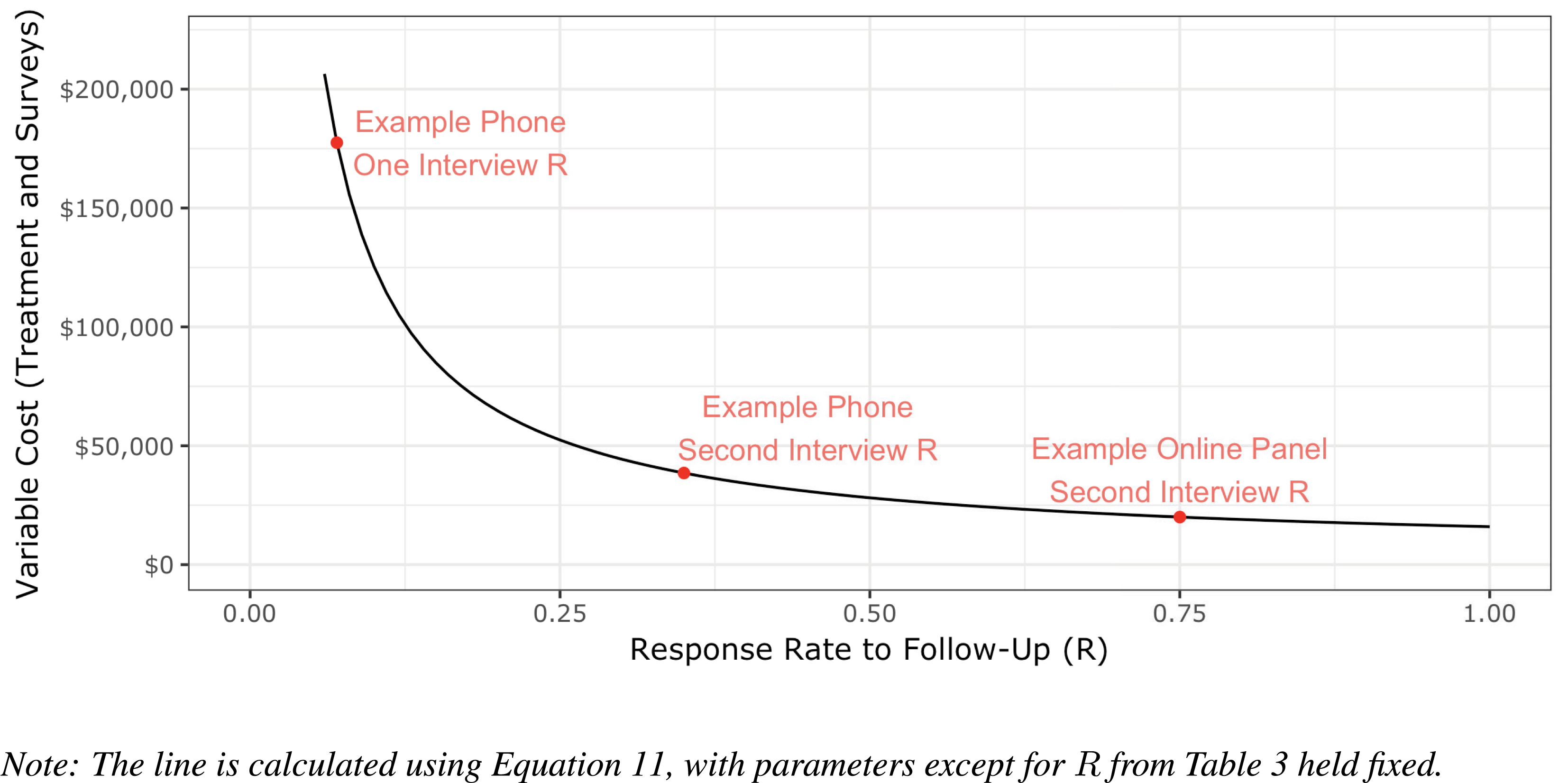
this reduces the cost of treatment in anticipation that more treated subjects can be surveyed. Figure 3 depicts this latter dynamic. Holding fixed the parameters in Table 3 and varying only the response rate to the follow-up survey, it shows how lower follow-up survey response rates increase costs.
How experiment costs decrease with higher survey response rates.

Again illustrating how the practices we study can complement each other, the baseline survey can also dramatically decrease the cost of using a placebo. When a placebo is used but a baseline survey is not, many placebo conversations are wasted on subjects whose outcomes cannot be measured because they will not complete a phone survey. A baseline survey can reduce placebo costs by reducing the number of placebo conversations wasted on nonresponders and, with prognostic pretreatment covariates, increasing the value of every successful placebo conversation.Footnote
6
The ratio of these costs is
 ${\textstyle \frac{(1-\unicode[STIX]{x1D70C}^{2})R_{1,T}}{R_{2,O}}}$
. With the parameter values in Table 3, a placebo costs about 1.8% of what it would cost to implement with traditional designs.
A baseline survey can also help researchers detect or attempt to adjust for differential survey attrition or improper implementation of a placebo.Footnote 7
3.2.3 Practice 3: Multiple measures analyzed as an index
Equation (11) showed how higher test–retest correlations
 $\unicode[STIX]{x1D70C}$
between baseline and outcome measurements increase efficiency. Due to measurement error, one item may have a small correlation between two survey waves even if the underlying attitude it measures is stable. However, when multiple measures of an attitude are collected and combined into an index, stability between survey waves can increase considerably (Ansolabehere, Rodden, and Snyder Reference Ansolabehere, Rodden and Snyder2008). This increase in stability can increase the precision of estimates dramatically, increasing efficiency.
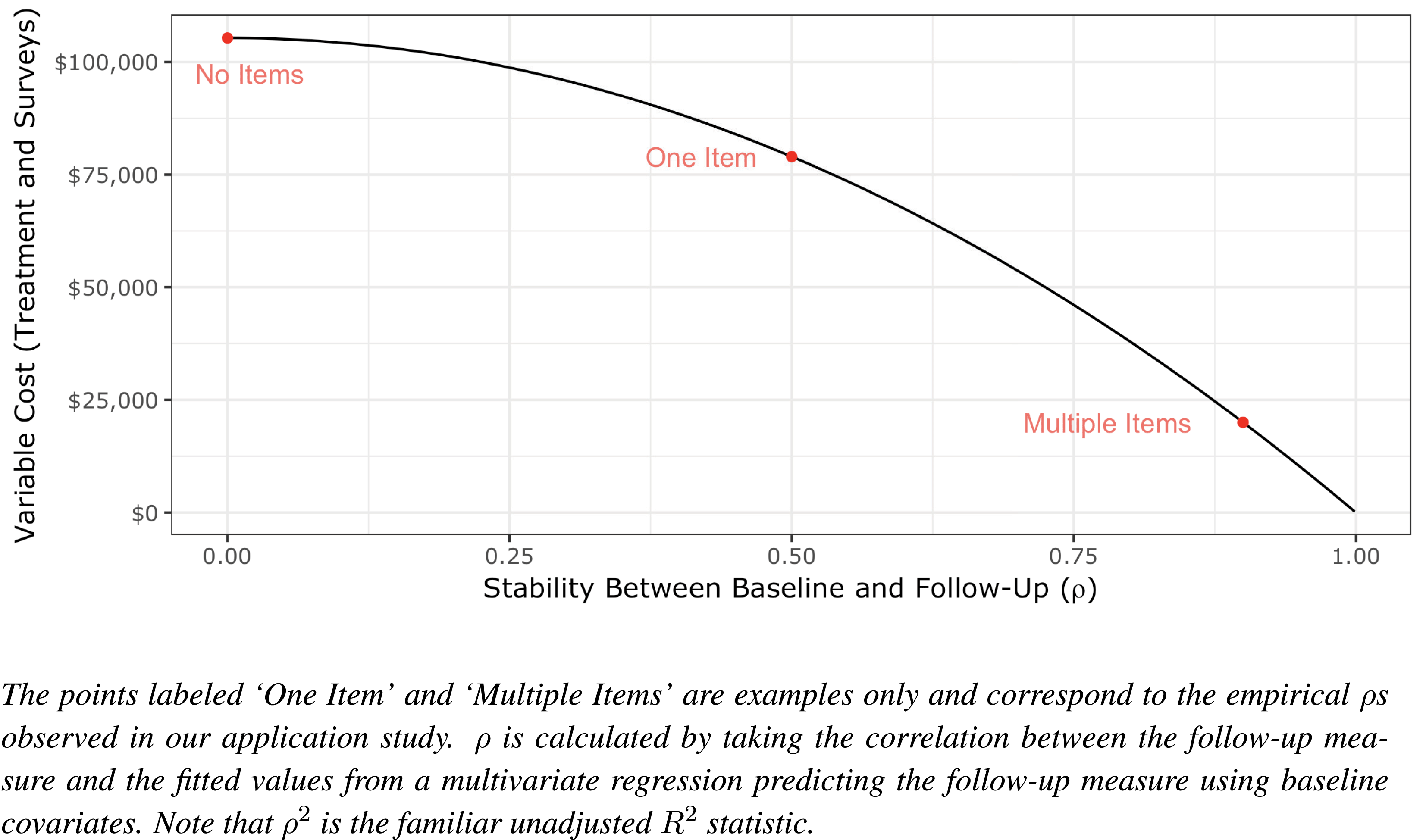
Empirical values from our application study illustrate the magnitude of these potential gains. In that study, analyzing an index of multiple items instead of only one item increases the test–retest correlation
 $\unicode[STIX]{x1D70C}$
to 0.9 from an average of 0.5. This corresponds to a more than threefold increase to 0.81 from 0.25 for the
 $\unicode[STIX]{x1D70C}^{2}$
used in Equation (11), and thus a more than threefold decrease in costs. Figure 4 shows these gains graphically. Without multiple measures, baseline surveys are less useful for reducing sampling error; the point corresponding to “One Item” in Figure 3 at
 $\unicode[STIX]{x1D70C}=0.5$
implies relatively modest cost savings over a completely unpredictive baseline (at far left). However, with multiple measures, baselines can reduce sampling error tremendously. Note that multiple measures can increase precision even when one item is stable, such as vote choice or partisanship can be; for example, increasing
 $\unicode[STIX]{x1D70C}$
from 0.9 to 0.95 would decrease costs by roughly half.
Although psychology research consistently collects multiple measures to form an index, Table 1 shows that this practice is rare in existing political science field experiments with survey outcomes. We suspect the reason has to do with survey mode, a point to which we turn now.
3.2.4 Practice 4: Online survey mode
The fourth practice we study is recruiting individuals to online surveys from a defined sampling frame, such as a list of registered voters (as in our empirical studies), list of all addresses (Jackman and Spahn Reference Jackman and Spahn2015), FEC donor lists (Barber, Canes-Wrone, and Thrower Reference Barber, Canes-Wrone and Thrower2017), list of physicians (Hersh and Goldenberg Reference Hersh and Goldenberg2016), or one of many others (see Cheung Reference Cheung2005). Online surveys can complement the practices studied above in three major ways.
First, online surveys can increase reinterview rates after baseline surveys, increasing
 $R_{2}$
. That is, we have observed
 $R_{2,O}>R_{2,T}$
, likely because the first survey can capture additional contact information for each respondent (e.g., an email address) and easily provide them incentives (e.g., a gift card). Increases in
 $R_{2}$
increase the value of baseline surveys. In our work so far, reinterview rates in this mode have sometimes exceeded
 $R_{2,O}=80\%$
. However, reinterview rates on the phone can be considerably lower; we have observed
 $R_{2,T}=35\%$
, similar to existing literature (see Online Appendix B).
Second, surveys that collect multiple measures can be cheaper to administer online than by telephone (that is, we have observed
 $S_{O,M}<S_{T,M}$
). For every question in a live telephone survey, an interviewer must read the question and record respondents’ answers. We expect telephone surveys rarely collect multiple measures for this reason. Online surveys rarely carry a high per-question cost. The
 incentives we have provided for surveys of over 50 questions are much smaller than quotes we received for telephone surveys of this length (see Online Appendix B).
Third, online surveys may have higher test–retest reliabilities, such that
 $\unicode[STIX]{x1D70C}_{O,M}^{2}>\unicode[STIX]{x1D70C}_{T,M}^{2}$
. In our first empirical study we observed larger
 $\unicode[STIX]{x1D70C}$
s for the same questions asked online than by telephone.
Such potential increases in
 $R_{2}$
and
 $\unicode[STIX]{x1D70C}^{2}$
and decreases in
 $S_{M}$
mean collecting outcomes by online panels have the potential to achieve the same precision for less cost than by other survey modes.Footnote
8
With this said, two major concerns about online surveys bear mentioning. First, when studies are conducted in other settings, many of these parameter values may change, resulting in different optimal designs (see, e.g., Section 4.3). Second, respondents to online surveys may prove less representative than those recruited with traditional modes. For this reason, we recommend recruiting respondents from an ex ante defined sampling frame. Existing evidence suggests online respondents recruited from a defined frame can be more representative than those who “opt in” to online surveys (e.g., Brüggen, van den Brakel, and Krosnick Reference Brüggen, van den Brakel and Krosnick2016). More importantly, being able to compare respondents to a defined frame facilitates empirical examination of how representative a sample is on observables. Researchers should also think critically about how unobservable characteristics of those who respond to any survey mode might affect their conclusions. With this said, because the representativeness of subjects recruited to online surveys is a special concern, we return to this topic with our first empirical study, presented in Section 5.
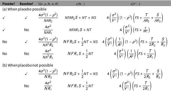
Variances and variable costs of alternative designs.

4 A Framework for Selecting Experimental Designs
Scholars wishing to conduct a field experiment with survey outcomes may encounter substantially different design parameters than those explored in the running examples and Table 3. In this section, we provide a framework for how to use the formulas we derived in the previous section to select more efficient and ethical designs. We also provide several examples of how scholars can apply this framework across diverse applications, to their particular questions and setting. These examples will also reinforce our argument that complementarities between these practices can produce large advantages.
Table 4 organizes our analytical results derived in the previous section. As we show, these formulas allow researchers to compute variances and costs of potential experimental designs as a generic functions of parameters in their settings under alternative permutations of the four design practices we have discussed. The notation in Table 4 corresponds to the same notation defined in Table 3. Table 4a gives the variances and costs of alternative designs depending on the presence or absence of a placebo, baseline survey, multiple measures, and online survey mode for cases when compliance can be observed and so a placebo is possible. The presence or absence of placebos and baseline surveys changes these formulas. Survey mode and the presence or absence of multiple measures may change parameters in these formulas but not the formulas. Table 4b gives the same but for settings where a placebo is not possible because compliance cannot be observed; these are derived in Online Appendix A.
4.1 Example 1: Door-to-door canvassing study in the United States
Figure 1 at the beginning of the paper previewed how a researcher could use our framework to determine the costs of each of sixteen ways to conduct a door-to-door canvassing study under a given set of empirical parameters. The results in Figure 1 follow from plugging in the parameters from Table 3 to the formulas in Table 4a. In that application, our framework found a design with variable costs approximately 98% lower than common designs. In the remainder of this section we show how our framework can be applied to a variety of other settings.
4.2 Example 2: Mailing information about members of Congress
In some settings, a placebo is not possible because compliance cannot be observed. Suppose a researcher wants to examine how individuals learn and retain information about their Members of Congress. A researcher might want to include individuals in many Congressional districts to expand the generalizability of the conclusions. A door-to-door canvass treatment would be difficult to deploy on this nationwide basis, but a mail experiment would be practical. However, one cannot easily observe whether a person opens a piece of physical mail, so a placebo could not be used. Table 4b gives formulas for alternative designs in situations where a placebo is not possible. To select the optimal design, we use these formulas and again use the values in Table 3, but substitute  corresponding to an example mail treatment with a marginal cost of

How experiment costs decrease with higher stability between baseline and follow-up outcome measurements.

Applying the framework when placebo not possible: mail example.

Figure 5 provides the results of applying our framework to this experimental design problem. Under these conditions, employing all three possible practices reduces variable costs from approximately  if none of these practices are used to approximately
 Interestingly, in this application our framework also surfaces that using each of two of these practices alone may actually increase variable costs.
4.3 Example 3: The World Bank studying a public health intervention in Liberia
Our motivating examples so far have considered how to study the effect of field treatments on political attitudes in the United States, but our framework is much more general. Moreover, it can show how different designs may be more optimal for researchers pursuing different aims in different contexts.
As an example of how our framework can be extended to a different setting, we consider a recent study by The World Bank examining how Ebola infections affected self-reported outcomes such as employment and schooling in Liberia (Himelein Reference Himelein2015). These outcomes were collected in a telephone panel survey.
Suppose these researchers wanted to conduct a field experiment in Liberia to estimate the effect of a public health worker visiting households providing public health information about avoiding Ebola on these outcomes. Our framework is first able to identify the key parameters of interest researchers must forecast to determine which designs would be optimal. In their Liberia study, researchers from the World Bank conducted five rounds of mobile telephone surveys (
 $F=5$
). The initial survey response rate (
 $R_{1,T}$
) was 28% and the follow-up telephone survey response rate (
 $R_{2,T}$
) was 73%. Indicative of the share of people who can be reached at home in Liberia when one knocks on their door, the contact rate in the face-to-face Afrobarometer survey conducted in May 2015 in Liberia (Isbell Reference Isbell2016) was 97%, so we assume a treatment application rate
 $A=0.97$
. However, suppose in Liberia an attempted visit from a public health worker is inexpensive given lower wages, such that
 but that online surveys would be much more expensive because many people do not have internet access and would need to be provided it
 For the sake of simplicity, we let online and telephone surveys have the same response rates (
 $R_{1,T}=R_{1,O},R_{2,T}=R_{2,O}$
) and let
 $V^{\ast }$
,
 $\unicode[STIX]{x1D70E}^{2}$
,
 $\unicode[STIX]{x1D70C}^{2}$
, and
 $S_{T}$
remain unchanged from Table 3.
Figure 6 applies our framework to this setting, examining the most feasible way to conduct this study. In this example, using all four practices we study would not be the most efficient option, nor would the traditional design in the literature. Instead, it would be a telephone survey with a baseline survey and placebo but without multiple measures, to keep the survey short.
Example results: variable costs for studying public health intervention in Liberia.

The results in Figure 6 could also help these researchers navigate more complicated trade-offs. Suppose a collaborating Non-Governmental Organization refused to implement a placebo condition. The researchers could now detect that conducting a baseline survey is not optimal given that there will be no placebo, even though a baseline survey was optimal when the placebo was present. Alternatively, suppose the researchers wanted to collect multiple measures of outcomes to match existing questionnaires. Our framework now suggests that conducting an online survey may be worth the additional cost, as the parameters we input assumed that a phone survey collecting multiple measures offered less cost savings on marginal costs than a short phone survey. These examples illustrate how our framework can surface subtle complementarities and trade-offs between these practices. Our framework also allows researchers to consider more traditional trade-offs. For example, suppose researchers considered using an online survey without providing internet access to those who did not have it, limiting the sampling frame to pre-existing internet users but eliminating the cost of providing internet access. Our framework would allow researchers to compute the money this choice would save and allow them to consider whether this cost savings was worth the potential bias and external validity limitations this would introduce.
4.4 Example 4: Comparing designs as parameters vary
This framework also allows researchers to consider how various design decisions might generalize as design parameters change. For example, what if a researcher has priors over a range of values a parameter may take and wants to test how design decisions may change across that range?
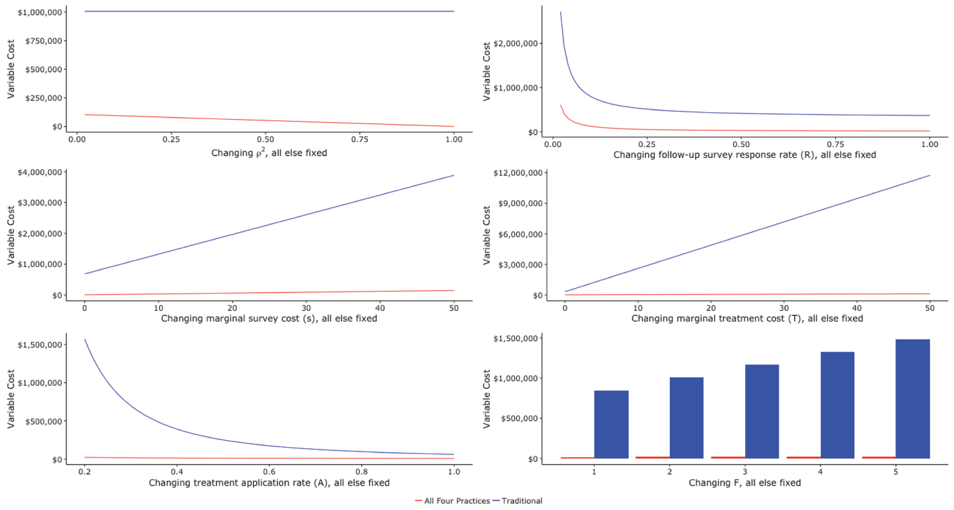
Figure 7 shows how a researcher conducting a door-to-door canvassing study like the one discussed in the running example could use our framework to compute how variable costs would change as each of the parameters the framework considers changes, holding all other parameters at their Table 3 level. In each of the six panels of Figure 7 we vary one of six parameters and show the cost of a study using the literature’s traditional design and a design using all four practices. Figure 7 thus demonstrates how our framework can help researchers select superior experimental designs under a wide variety of circumstances. That the design using all the practices we study is consistently superior for these ranges of parameter values also suggests that scholars in a variety of settings may benefit from considering these practices.
How variable costs change with parameters.

4.5 Example 5: Internalizing ethical externalities
Many have expressed concern that large field experiments might change collective political outcomes (Michelson Reference Michelson2016). When field experiments require trying to change tens of thousands of individuals’ minds, this concern is especially salient. Our framework is also able to help researchers internalize such potential ethical externalities. Suppose a researcher plans to study a treatment administered by phone that attempts to persuade registered voters on an issue with a marginal cost of attempting treatment
 $T$
of
 (e.g., a “cost per dial”). Further suppose this researcher perceives the ethical externality of attempting each conversation as approximately
 This would increase the marginal cost of attempting treatment
 $T$
from
 to
 Re-computing the variable costs of these experiments, the experiment not using any of the four practices would go from approximately
 to
 in variable cost, reflecting an ethical externality of
 The experiment using all four of these practices would go from approximately
 to
 in cost, reflecting an ethical externality of

This example establishes two points. First, this example shows the potential advantages in variable cost we have studied can also confer an ethical advantage: because under many conditions using some of these practices means many fewer individuals need to be treated, researchers can reduce the scope of their potential to influence real-world outcomes. More generally, this example shows how our framework can be used to consider a wide variety of potential issues that arise when considering alternative field experimental designs. For example, researchers who assigned a subjective value of  to the robustness to differential attrition a baseline survey provides could integrate this value into our framework as well.
5 Empirical Study: Representativeness of US Registered Voters Recruited By Mail To An Online Panel
We now present two empirical studies that examine how the practices we study perform in real applications.Footnote 9 First, we examine the representativeness of a sample recruited to an online panel survey from a defined sampling frame. Scholars may wonder how subjects recruited to one or more rounds of online surveys may differ from subjects recruited by the literature’s traditional means, a single round of phone surveys. Our first empirical study considers this issue in detail. Specifically, we recruited US registered voters by mail to two rounds of online surveys and compared their representativeness to that of one and two rounds of phone survey respondents, using both the original sampling frame and other surveys as benchmarks.
We expected online surveys recruited from an ex ante defined frame to yield fairly representative but slightly more educated samples. Debates continue about the generalizability of “opt in” online survey samples recruited by online ads (e.g., Hill et al. Reference Hill, Lo, Vavreck and Zaller2007), but research has generally found that surveys administered online are fairly representative when their samples are recruited from ex ante well-defined sampling frames (Brüggen, van den Brakel, and Krosnick Reference Brüggen, van den Brakel and Krosnick2016), with the exception that online samples tend to be slightly more educated on average given that more educated people are more likely to have internet access (Hall and Sinclair Reference Hall and Sinclair2011). However, existing research that considers the representativeness of online samples typically focuses on particular areas that may yield idiosyncratic results (e.g., Barber et al. Reference Barber, Mann, Quin Monson and Patterson2014; Collins and Rosmarin Reference Collins and Rosmarin2016) and often does not compare results to alternative recruitment methods in the same samples. We therefore sought to gather additional data on this question.
To consider the representativeness of online survey samples empirically, we randomly assigned a random sample of US registered voters to a telephone survey or to an online survey recruited by mail. This allows us to assess the general representativeness of this design on an absolute basis and in comparison to current practice. In addition, we used this nationwide exercise to inform the example parameter values used in Table 3 and our running examples; see Online Appendix B for discussion. (We fully expect these parameters would differ in nonrandom samples selected for particular studies.)
In early 2016, we purchased a national random sample of the publicly available list of registered voters, observed demographics available on the voter file, modeled demographics available from our data vendor, their mailing address, and, if available, their landline and mobile telephone numbers. This starting sample provides our first benchmark for representativeness. We then randomly assigned these voters to mail-to-online or phone modes and conducted the surveys. See Online Appendix Section C.1 for details on the data, random assignment procedures, and survey recruitment procedures. One note described further in the Online Appendix to which we want to draw attention is that subjects’ race is only observed in some states; it is the product of a statistical model in other states, and therefore we call this variable “Modeled Race.”
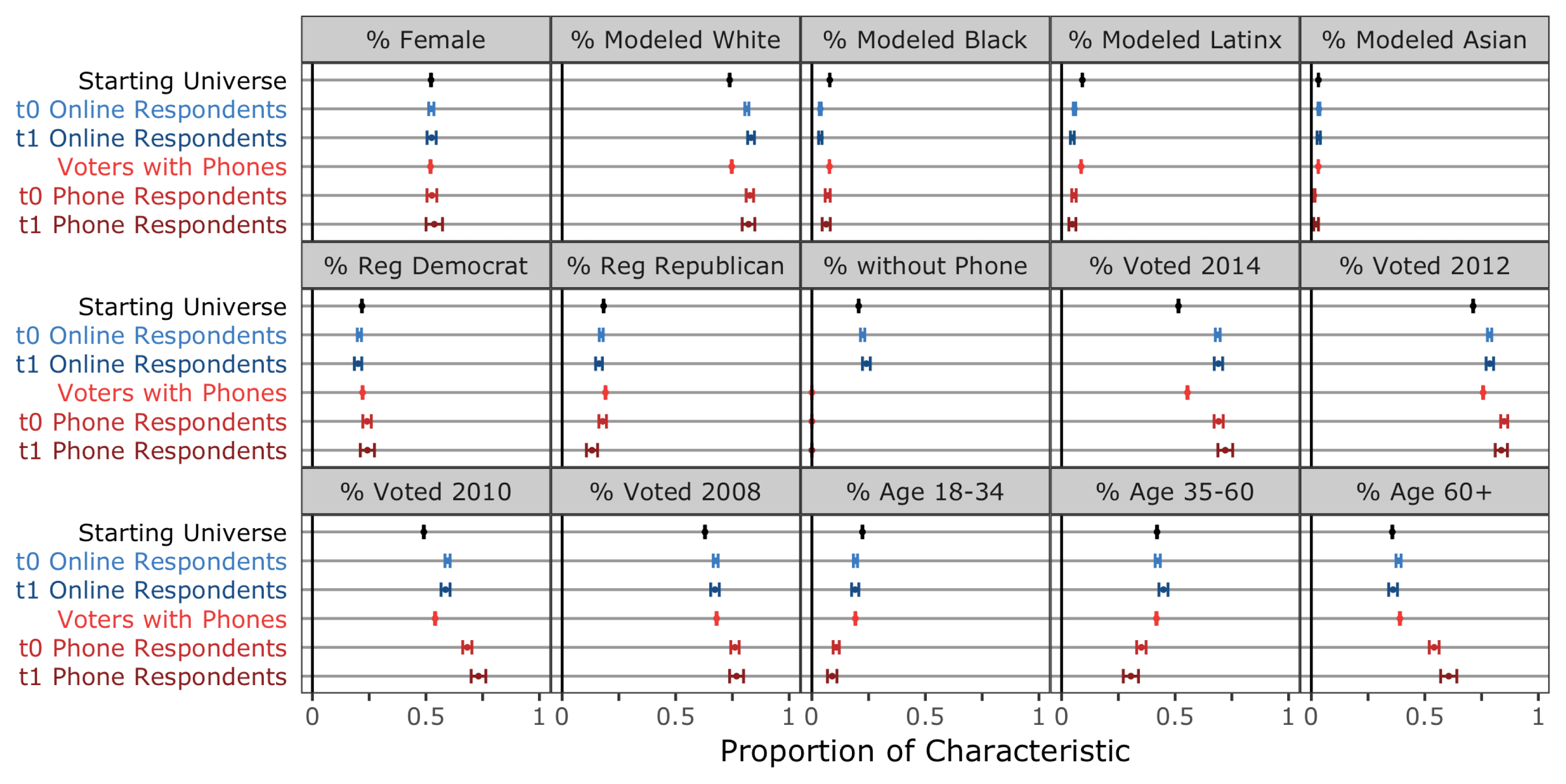
Average administrative data values for sampling frame and respondents.

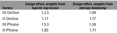
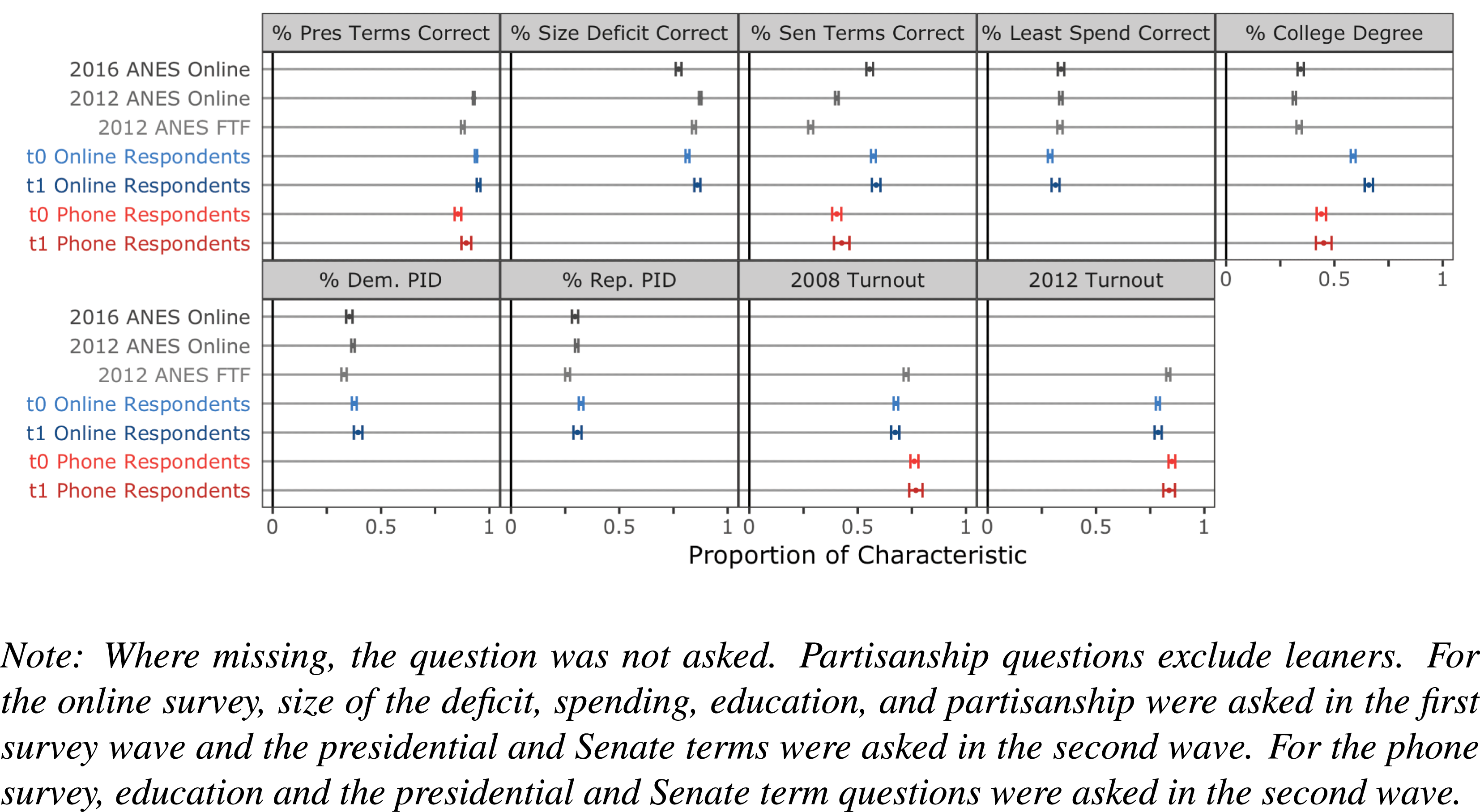
We first compare the administrative data available for the entire sampling frame to the data for just those who completed the baseline (“t0”) and follow-up (“t1”) online and phone surveys. Figure 8 shows the proportion of various characteristics present in these subsamples. (Table OA2 in Online Appendix reports point estimates.) Unsurprisingly, neither online nor phone respondents match the sampling frame exactly on every covariate, nor is either mode superior on every covariate. However, one way to assess the overall representativeness of each sample on observable characteristics is to compute the loss in efficiency that results when each sample is weighted back to the sampling frame, or the design effect (Kish Reference Kish1965). To calculate the design effects for each mode, we calculated survey weights using entropy balancing (Hainmueller Reference Hainmueller2012) and logistic regression using gender, modeled race, party identification, 2008, 2010, 2012, and 2014 voter turnout, age, and age squared. Table 5 shows the design effects for each method. A design effect of 1 would indicate perfect representativeness on observables; larger design effects indicate larger differences between the sampling frame and sample on observables.Footnote 10 Overall, both online survey waves had smaller design effects than the sample of individuals who responded to either one or two phone surveys.Footnote 11 With this said, we only have access to a limited number of variables on the US voter file, and further research with access to other variables would be of interest.
Design effects of online and phone surveys and panels.

We also compare these samples to the 2012 ANES and 2016 ANES Pilot Studies in Figure 9, some of which were conducted online as well.Footnote 12 We limit the ANES to only registered voters to match the sampling frame from our online survey. We then compare the sample on several questions that overlap: political knowledge (size of federal deficit and relative size of U.S. federal spending), party identification, reported education, and validated voter turnout (for the 2012 ANES face-to-face sample).Footnote 13 As expected, our online survey respondents are slightly more likely to be well-educated, politically active, and informed, but otherwise generally match the 2012 and 2016 ANES samples. (Table OA3 in Online Appendix reports point estimates.)
Covariates collected in 2012 and 2016 ANES, telephone, and online surveys.

Our finding that online survey respondents in the United States appear to be somewhat more educated, active, and informedFootnote 14 underscores a broader need for caution for all researchers using field experiments with survey outcomes: researchers should think critically about how respondents to any survey might differ on both observable and unobservable characteristics in their particular setting. For example, some theories would predict that relying on estimates from a sample with higher levels of education and information might lead to underestimates of population average treatment effects when studying political persuasion (e.g., Zaller Reference Zaller1992), a fact political scientists studying persuasion with field experiments with survey outcomes should bear in mind. More generally, the representativeness of different survey modes is likely to vary across settings in ways that will be specific to these settings and of which researchers should remain cognizant. By beginning with a defined sampling frame, however, researchers can better empirically examine representativeness on at least observable characteristics. In addition, researchers should be cognizant of whether the mode of their treatment interacts with the mode of their survey; for example, subjects recruited to a phone survey may be especially susceptible to persuasion by phone.
In summary, these data provide cautious optimism that online panel surveys can be capable of recruiting subjects that compare favorably to the representativeness of subjects recruited by phone. However, our findings also reinforce that researchers should think critically about how survey respondents might differ in their particular settings in ways relevant to their research questions.
6 Application Study: Door-to-Door Canvassing on Abortion
In this section we report an original study of a door-to-door canvassing experiment deploying all four of the practices we study. This application study illustrates two main points. First, readers may wonder whether it is logistically feasible to combine some of the practices we study. This application study establishes that an experiment employing all four of these practices is practical to execute and that it does indeed yield the efficiency advantages our framework indicates. Second, this study helps assuage potential concerns that experiments that conduct pretreatment baseline surveys are especially prone to demand effects. An experiment with a baseline survey involves multiple interactions between researchers and subjects, introducing the possibility that subjects in the treatment group will draw a connection between the surveys and treatment and report on the surveys what they believe those responsible for the treatment want to hear. However, this study estimated a precise null effect.
During 2015, volunteers from the Los Angeles LGBT Center’s Leadership LAB went door to door in Los Angeles County seeking to increase support for safe and legal abortion and attempting to reduce stigma toward women who have had abortions. The conversations lasted roughly 10 minutes on average and involved canvassers asking subjects to tell stories about when subjects had made mistakes in their relationships.
We worked with the Los Angeles LGBT Center to deploy an experiment to measure the effects of these conversations that used all four of the practices we have studied. First, the Los Angeles LGBT Center selected LA County neighborhoods that had voted against expanded abortion access in prior ballot initiatives and provided us the publicly available data on registered voters in these neighborhoods. We recruited these voters to an online survey panel via mail sent to the address at which they were registered to vote. 1,982 subjects completed the baseline survey. Most survey items were unrelated to abortion. Next, we randomly assigned respondents to receive an abortion-focused canvass (treatment) or to a recycling conversation (placebo), blocking on an index of baseline responses. Volunteers then knocked on subjects’ doors. Regardless of condition, they first identified subjects and marked them as compliers. Canvassers then delivered the treatment corresponding to the subject’s random assignment, either the abortion or placebo conversation.Footnote 15 Online Appendix D reports intervention details. One week after canvassing occurred, we invited subjects who were successfully reached at the door (compliers) to the follow-up survey via email. We again invited the same subjects to participate in a second follow-up survey five weeks after canvassing took place.
Observed design parameters were consistent with expectationsFootnote
16
and reinforce the opportunities for experimentation the four practices we study make available. In all, the surveys cost approximately  using the design with all four practices, but would have cost approximately
 with traditional designs. The design also only required Los Angeles LGBT Center volunteers to contact approximately 450 voters, but had the same precision as would a study using the traditional design if they had contacted approximately 46,000 voters. To reach 46,000 voters, Center volunteers would have needed to continue canvassing for over a decade at their same pace; our study took them a few days.
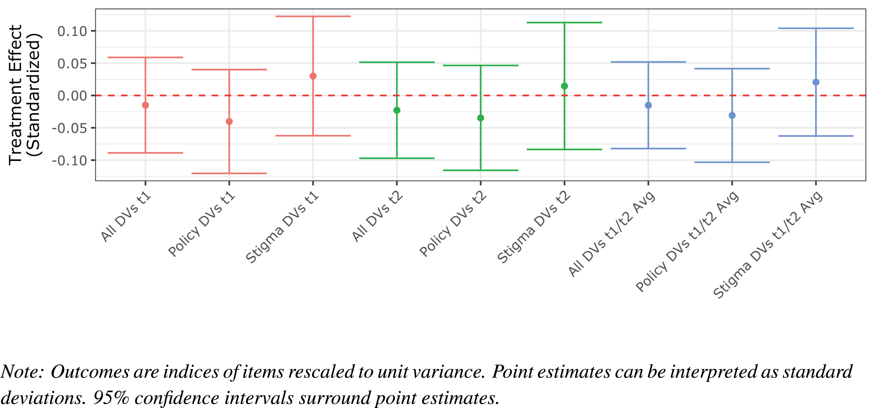
To estimate treatment effects on answers to the follow-up survey, we use a linear regression with an index of follow-up survey items as outcomes and the pretreatment answers to those items as controls. Standard errors are cluster-robust, with clustering at the household level. The outcome indices were computed by taking the first factor from factor analysis and rescaling them to a standard deviation of 1. We show the results for three dependent variables: an index of all the abortion items, an index of just the policy-relevant items, and an index of just the stigma-relevant items. The outcomes are measured for just the first posttreatment survey, just the second posttreatment survey, and an average of both posttreatment surveys (to further reduce measurement error). Online Appendix D.3 gives more detail. These analysis procedures were pre-registered.
Results indicate the treatment effect as a precisely estimated zero on all outcomes: the confidence intervals rule out positive effects of approximately 0.05 standard deviations, which is half the size conventionally considered “small.” Figure 10 shows these results. Online Appendix D reports balance checks and representativeness assessments.
Treatment effect estimates of canvassing on abortion attitudes.

In addition to demonstrating that these four practices are feasible to deploy in tandem, this study’s null result is encouraging for the validity of studies using these practices that find non-null results. One might worry that surveying subjects multiple times about the topic of an experiment necessarily introduces demand effects; subjects may make the connection between the online surveys and the treatment and adjust their survey responses to satisfy the researchers even if their attitudes did not change. This application study’s null result suggests these practices are capable of precisely estimating null treatment effects.
7 Concluding Discussion
The use of randomized experiments and survey-based research in the social sciences has mushroomed. Together with rising interest in these methodologies, many scholars have begun to conduct field experiments with survey outcomes: experiments where outcomes are measured by surveys but randomized treatments are delivered by a separate mechanism in the real world. However, challenges familiar to experimental researchers and survey researchers—survey nonresponse, survey measurement error, and treatment noncompliance—mean that common designs for field experiments with survey outcomes are extremely expensive and pose ethical challenges. In this paper, we showed that four practices uncommon in such experiments can yield particularly large gains in efficiency and robustness when they are used in combination. In some settings, the magnitude of these efficiency gains is extremely large. For example, the modal political science field experiment with survey outcomes in published work is a door-to-door canvassing experiment among registered voters in the United States. But to conduct a well-powered experiment using designs common in the literature, researchers in many settings may well require budgets larger than that of the entire 2016 ANES. However, using all of the practices we study can decrease an experiment’s variable costs to a level doctoral dissertation improvement grants could cover.
This paper also developed a framework that will help researchers select the design that is most optimal in diverse settings where treatment costs, survey costs, survey response rates, and other parameters may change. This framework identifies the key parameters that determine an experiment’s variable costs and allows researchers to examine the feasibility of a range of possible designs given these parameters. As we discussed, this framework is widely applicable and easily extensible. For example, researchers could use it to internalize the ethical externalities of treating many subjects or quantify the costs of introducing design practices expected to increase robustness. To accompany this paper, we are also making code available that implements this framework.
Although we are optimistic about the potential applications of the practices we study, several open questions remain. First, all experiments with survey outcomes only estimate effects for individuals who both receive the treatment (compliers) and agree to be surveyed (reporters). Data from our application study shown in Figure OA2 in Online Appendix suggests complier reporters are not highly unrepresentative on observables. Nevertheless, generalizing from these local average treatment effects to population treatment effects requires additional assumptions (Hartman et al. Reference Hartman, Grieve, Ramsahai and Sekhon2015). Although these limitations are theoretically similar regardless of the design used, the empirical representativeness of compliers under this design is a clear question for future research. With this said, future research seeking to benchmark the use of survey outcomes in field experiments against behavioral benchmarks (such as precinct-randomized experiments) may be able to take advantage of our framework to reach more precise survey-based estimates for validation.
Second, baseline surveys may have unintended effects that produce bias or reduce external validity. For example, answering survey questions about a topic might change how people later process information about it, such as by increasing attentiveness (e.g., Bidwell, Casey, and Glennerster Reference Bidwell, Casey and Glennerster2015). Most evidence on this phenomenon is either from developing countries or several decades ago, so it is unclear to what extent present-day populations in developed countries would exhibit such effects. Individuals who answer a survey twice may also be systematically different than those who answer once, as our first empirical study found for phone surveys. This is an important area for future research, with designs readily available in classic psychometric literature (e.g., Solomon Reference Solomon1949).
Answering multiple follow-up surveys after a treatment may also produce biased estimates of treatment effects’ persistence over time if subjects remember how they answered particular questions in a previous survey wave. Existing survey and field experiments that track long-term effects (e.g., Coppock Reference Coppock2016) often observe rapid decay in treatment effects, so this bias clearly does not always exist. Refreshment samples or randomly staggered interview times could help address this possibility.
The particular implementation of each of the practices we studied may also be open to improvement. For example, one possible extension to conducting a baseline survey is to conduct multiple baseline waves prior to treatment. Multiple baselines would further increase stability (increasing
 $\unicode[STIX]{x1D70C}^{2}$
) (McKenzie Reference McKenzie2012) and could help identify subjects even more likely to participate again (increasing
 $R$
). Our framework could be readily applied to determine whether the costs of an additional baseline wave prior to treatment would outweigh these benefits.
We look forward to future research extending these practices and our framework and employing them to shed light on a variety of substantive questions.
Supplementary material
For supplementary material accompanying this paper, please visit https://doi.org/10.1017/pan.2017.27.
Appendix
Example experimental design using all four practices.