

I. Introduction
As corporate insiders possess information that is not available to any other market participants, insider trading has attracted interest from academics and regulators to understand the impact of this trading. On the one hand, insider trades carry information, making prices more efficient and facilitating price discovery (Manne (Reference Manne1966), Carlton and Fischel (Reference Carlton and Fischel1983)). Insiders possess intimate knowledge of the fundamental value of the firm and so could trade to push prices toward this “true” valuation. On the other hand, insider trades can harm uninformed traders and damage market liquidity (Ausubel (Reference Ausubel1990), Fishman and Hagerty (Reference Fishman and Hagerty1992), Leland (Reference Leland1992), and Bebchuk, Cohen, and Ferrell (Reference Bebchuk, Cohen and Ferrell2002)). Regulators aim to impose insider-trading restrictions, which reduce the adverse market effect but retain the efficiency effects of insider trading. In this respect, regulators wish to restrict trading on foreknowledge of material information but at the same time to allow trading on short-term mispricings that arise due to market misinterpretation of public information releases.
In this article, we aim to understand the source of insiders’ information advantage when trading under tight regulatory restrictions.Footnote 1 We build a simple model and test empirical predictions of whether insiders trade on foreknowledge of material information or react to short-term mispricing. Contrary to the existing literature concluding that insiders trade on foreknowledge of future material information (see Ke, Huddart, and Petroni (Reference Ke, Huddart and Petroni2003), Cheng, Navar, and Rajan (Reference Cheng, Navar and Rajan2007), Cohen, Malloy, and Pomorski (Reference Cohen, Malloy and Pomorski2012), Ali and Hirshleifer (Reference Ali and Hirshleifer2017), and Akbas, Jiang, and Koch (Reference Akbas, Jiang and Koch2020)), we find little evidence of illegal insider trading on material information in the post-Sarbanes-Oxley (post-SOX) period. Insider trades correlate with future returns, but they rely on short-term mispricing.
Differentiating whether insiders trade on foreknowledge of material information or react to short-term mispricing is a difficult task. The existing literature often relates the ability of insider trades to predict future returns as evidence of insiders trading on foreknowledge of material undisclosed information (see, e.g., Huddart et al. (Reference Huddart, Ke and Shi2007), Cohen et al. (Reference Cohen, Malloy and Pomorski2012), and Akbas et al. (Reference Akbas, Jiang and Koch2020)). This approach may be misleading since informed traders can make profits on their trades even when they legally exploit mispricing stemming from the market’s misinterpretation of publicly disclosed information. For example, suppose the market misinterprets an earnings announcement and overreacts. Shortly after the earnings announcement, an insider decides to sell to exploit the mispricing. This trade is not based on any foreknowledge of material information because the insider uses the earnings information that has just been released to the public. The trade is not illegal. Yet, the insider profits from the sale because the overpricing will eventually be reflected in a lower stock price, which leads to a negative future abnormal return. This example illustrates that insiders do not need to trade on foreknowledge of material private information for their trading to be profitable and for the trade direction to forecast future stock returns. As a result, it is essential to identify and filter out insider trading on mispricing.
In order to separate the two sources of information, one needs a reliable measure of mispricing, which is a task without a suitable direct solution in the empirical finance literature so far. We opt for a highly correlated proxy: an alternative group of informed traders, whom we call arbitrageurs, who trade predominantly on short-term mispricings arising after public news releases. To fully understand interactions between arbitrageurs’ and insiders’ trading, we build a simple theoretical model. This model guides our empirical identification strategy.
In line with our research question, our model works with two types of information and two types of informed traders. Arbitrageurs possess information about short-term mispricing (hereafter, short-term information) arising after public news. An example of such information is arbitrageurs’ ability to better estimate fundamental values of stocks after public news releases and to identify market under- or over-reactions. Anybody with a special information-processing skill could profit on this type of information without breaking trading rules. The short-term information is also in possession of an insider—he/she is also able to spot mispricing. In addition, the insider, but not arbitrageurs, has access to foreknowledge of material information (hereafter, long-term information). Future new product releases, asset sales, acquisitions, etc., are examples of information that falls into this category. Trading on the long-term information is regarded as illegal, as it is material in the true sense; it is not released in a public announcement and is price-sensitive.Footnote 2
It is noteworthy to highlight that trading on the short-term information in the model is equivalent to trading on mispricing, which takes advantage of public information and is not illegal. In contrast, trading on the long-term information relies on foreknowledge of material information, and this type of information is not available to arbitrageurs. As we are interested in unveiling whether the insider does take advantage of his/her privileged access to the long-term information, we contrast predictions of two benchmarks: a benchmark where the insider abstains from trading based on the long-term information to avoid legal prosecution versus a benchmark where the insider trades optimally by taking into account all available information. Because the insider’s information set is richer than that of arbitrageurs in the latter benchmark, any disagreement between the insider and arbitrageurs translates into a strict advantage for the insider. As a result, the insider takes advantage of buying or selling pressure coming from arbitrageurs who trade on the basis of short-term information only. Hence, in the case, the long-term and short-term information disagree, the latter benchmark predicts that the insider’s demand is contrarian to the short-term information and arbitrageurs’ demand. This is not the case for the former benchmark, where the insider trades only on the short-term information. These contrasting predictions help to identify whether the insider uses the long-term information when trading or not.
In our empirical analysis, we use short interest to proxy the demand of arbitrageurs. We argue that this is a reasonable strategy due to the nature of short sellers’ trading around earnings announcements. Short sellers are informed traders with strong incentives to profit on their information advantage who trade on mispricing when the market over- or under-reacts to public news.Footnote 3 McLean, Pontiff, and Reilly (Reference McLean, Pontiff and Reilly2020) show that short sellers are the only group of influential market participants, except insiders, who build positions in agreement with 130 anomaly strategies which have been shown to predict the cross-section of stock returns. Engelberg, Reed, and Ringgenberg (Reference Engelberg, Reed and Ringgenberg2012) show that short-sellers’ information advantage around earnings announcements indeed comes from their superior ability to analyze publicly available information. It is also important to note that short-sellers’ investment horizon is usually relatively short, which makes them unlikely to be trading on foreknowledge of future material information.Footnote 4
Using a sample of insider trades in U.S. stocks shortly after earnings announcements from 2006 until 2017, we conclude that although corporate insiders’ purchases and sales do forecast future returns, insider sales are based on the short-term overpricing only. We document that insiders tend to sell overwhelmingly in agreement with short sellers even for more informed non-routine (opportunistic) insider transactions (Cohen et al. (Reference Cohen, Malloy and Pomorski2012)). The average monthly profit of an insider sale when insiders agree with short sellers is $5,391, while the profit is statistically insignificant when insiders and short sellers disagree. Insider purchases sometimes take advantage of the long-term information, they forecast future returns when short sellers disagree by selling heavily. However, insider purchases are 4 times smaller than sales and disagree with intensive short selling only in about 2% of all firm-quarters in our data set. So, the economic effect of insiders exploiting undisclosed material information when buying is small, and their profit is statistically insignificant.
We also test whether it is the tighter SOX regulation that is behind the insiders’ abstaining from selling on foreknowledge of private information. We extend our sample by utilizing Compustat short-selling data and compare the pre- versus post-SOX periods.Footnote 5 We show that insiders sell on foreknowledge of material information before SOX; insider sales predict negative future returns when they disagree with short sellers on the direction of trading. This predictive power decreases significantly after SOX. Insiders’ dollar profits when selling are significantly higher before than after SOX. We conclude that tight regulatory restrictions after SOX are effective in mitigating insider trading on foreknowledge of material information. Insider trading still correlates with future returns but is highly aligned with short sellers’ trading; insiders choose not to use more information than is in the short sellers’ possession.
We contribute to the insider trading literature by adding to the discussion on what kind of information insiders use when trading under tighter regulation. Literature suggests that insider trades are motivated by either foreknowledge of future material information (Ke et al. (Reference Ke, Huddart and Petroni2003), Cheng et al. (Reference Cheng, Navar and Rajan2007), Cohen et al. (Reference Cohen, Malloy and Pomorski2012), and Ali and Hirshleifer (Reference Ali and Hirshleifer2017)) or by public information (Jenter (Reference Jenter2005), Kolasinski and Li (Reference Kolasinski and Li2010), and Alldredge and Cicero (Reference Alldredge and Cicero2015)). We contribute by using the interaction of insiders’ and short-sellers’ demands to detect insider trading on foreknowledge that is not available to short sellers. Our strategy can distinguish insider trading that exploits mispricing after public news releases from insider trading on foreknowledge of material information.
We are not the first to explore the question of the information source of insider trading. Piotroski and Roulstone (Reference Piotroski and Roulstone2005) argue that insiders use both types of information advantage. Our results are different in three ways. The first difference is in how we identify the trading on mispricing. Piotroski and Roulstone (Reference Piotroski and Roulstone2005) use the book-to-market ratio. While the book-to-market ratio could be regarded as a mispricing indicator, it also reflects other firm characteristics, such as the degree of distress, growth opportunities, or expected returns.Footnote 6 We instead rely on orders of traders who are known to play the role of arbitrageurs, trading to exploit mispricing after public news releases, which is a more refined, precise, and cleaner measure of short-term mispricing, measured on a daily frequency. We also highlight the disagreement between insiders and arbitrageurs and its correlation with future returns, which is at the core of our identification strategy.
Second, our samples are different. We use a sample that follows the SOX Act in 2002, while the sample in Piotroski and Roulstone (Reference Piotroski and Roulstone2005) ends in 2000. Finally, our research design allows us to condition on the direction of trading and show that only insider purchases, but not insider sales, are, in some cases, based on foreknowledge of future material information. This highlights the increased legal prosecution costs since 2002 and contrasts with papers documenting that pre-SOX insiders sell on knowledge of economically significant forthcoming accounting disclosures (Ke et al. (Reference Ke, Huddart and Petroni2003)). We show that insider trading restrictions are largely effective and insiders sell mostly in line with short sellers on short-term mispricing.
We also contribute to empirical literature which finds little evidence that insider sales, in contrast to insider purchases, are profitable (Lakonishok and Lee (Reference Lakonishok and Lee2001), Jeng, Metrick, and Zeckhauser (Reference Jeng, Metrick and Zeckhauser2003)). The main explanation for these findings is that insiders often sell for liquidity and/or diversification reasons and do not use their information advantage (Lakonishok and Lee (Reference Lakonishok and Lee2001), Cheng et al. (Reference Cheng, Navar and Rajan2007)). Cohen et al. (Reference Cohen, Malloy and Pomorski2012) show that excluding repetitive insider selling that is more likely due to liquidity/diversification reasons leads to remaining opportunistic insider sales to become profitable. They conclude that opportunistic insider sales are driven by foreknowledge of future material information. In contrast, our analysis suggests that opportunistic insider sales are profitable due to taking advantage of short-term mispricings arising after public news releases rather than due to foreknowledge of future material information. In a similar vein to Cohen et al. (Reference Cohen, Malloy and Pomorski2012), Akbas et al. (Reference Akbas, Jiang and Koch2020) highlight short-horizon insiders as better performing in predicting future returns than long-horizon insiders because their trades are more unexpected and more informed. However, Akbas et al.’s classification of short-horizon insiders still does not answer the question of what type of information is used by these insiders. Short-horizon insiders may rely on short-term mispricing rather than on foreknowledge of material information.
Our article is also related to the literature on the relationship between short sales and trades of other informed investors. Massa, Qian, Xu, and Zhang (Reference Massa, Qian, Xu and Zhang2015) explore how the potential presence of short sellers affects the incentives of insiders to trade on negative material information. They show that the intensity and speed of insider sales in a given month increase with higher short-selling potential in the previous month. They conclude that insiders and short sellers compete for trading on foreknowledge of the same private information. Wang, Wang, Wei, Zhang, and Zhou (Reference Wang, Wang, Wei, Zhang and Zhou2022) show that the threat of short selling reduces opportunistic insider sales and argue that short sales exert discipline for insiders. Chakrabarty and Shkilko (Reference Chakrabarty and Shkilko2013) examine short sellers’ informativeness regarding recently completed insider sales and show that short selling by non-market makers increases on days of insider selling. In contrast to these papers, we focus on the information content of insider trades. We differentiate information sets of insiders and short sellers and use the differences to identify the nature of insiders’ information advantage.
The remainder of the article proceeds as follows: Section II introduces our model and derives our testable hypotheses. Section III describes the data. Section IV presents our main findings, Section V compares pre- versus post-SOX periods, and Section VI discusses our key assumptions and their consequences for interpretation of the results. Section VII concludes.
II. Theoretical Predictions and Testable Hypotheses
A. A Simple Model
We develop our testable hypotheses by relying on a simple model of insider trading with an insider who possesses short-term information (i.e., information stemming from mispricing, arising after misinterpretation of a public announcement by the market) and long-term information (i.e., foreknowledge of material private information). The insider trades along with arbitrageurs who possess only the short-term information. We assume that the long-term information is truly private: it is undisclosed, price-sensitive, and in possession exclusively by the insider. The insider could be prosecuted if trading on this long-term information. The short-term information is also available to arbitrageurs because they have a superior ability to process public news releases relative to the rest of the market. Anybody who can do this would be classified as an arbitrageur in our model. Trading on the short-term information is not illegal because it is based on public information.
In order to test our research question of whether insiders (illegally) trade on foreknowledge of long-term material information, we derive two benchmarks and formulate testable predictions corresponding to each benchmark. In the first benchmark, we assume that the insider manager abstains from trading based on the long-term information to avoid legal prosecution, and denote it the “No-Long-term-Information” (
$ NLI $
 ) benchmark. In the second benchmark, denoted as the “All-Information” (
$ AI $
 ) benchmark, we assume that the insider trades optimally by taking into account both the short-term and long-term information. This benchmark shows insider trading patterns in the limiting case when the insider does not care about prosecution.
The market is populated by four types of market participants: a competitive market maker, a single insider trader,
$ n $
 identical arbitrageurs, and a group of liquidity traders. The model has three periods, which we index as
$ t\in \left\{\mathrm{1,2,3}\right\} $
 . Consider a firm with an initial fundamental value of
$ {v}_0 $
 , which is publicly known. We assume that the firm has one share of stock outstanding and its price is
$ {p}_0={v}_0 $
 . The insider initially holds
$ \eta $
 shares. In period 1, the insider and arbitrageurs learn that the fundamental value of the firm changes from the initial
$ {v}_0 $
 to
$ {v}_0+{v}_1 $
 , where
$ {v}_1\sim N\left(0,{\sigma}^2\right) $
 . Here,
$ {v}_1 $
 innovation represents the short-term information. The market maker knows only the distribution of
$ {v}_1 $
 . Moreover, in period 1, the insider also learns that the fundamental firm value will change from
$ {v}_0+{v}_1 $
 to
$ {v}_0+{v}_1+{v}_2 $
 , where
$ {v}_2\sim N\left(0,{\sigma}^2\right) $
 . Here,
$ {v}_2 $
 innovation represents the long-term information. We assume that
$ {v}_1 $
 and
$ {v}_2 $
 are independent.Footnote
7 The information about the realization of
$ {v}_2 $
 is not available to the arbitrageurs in period 1; they can only observe the distribution of
$ {v}_2 $
 . In period 2, the value of
$ {v}_2 $
 becomes known to the arbitrageurs but not to the market maker. This means that the long-term information becomes after some time known to some market participants, in addition to the insider. In period 3, the firm is liquidated and the dividends are paid to all shareholders at price
$ {p}_3={v}_0+{v}_1+{v}_2 $
 .
In periods 1 and 2, some liquidity traders need to trade
$ {u}_1 $
 and
$ {u}_2 $
 shares of the stock to cover their private liquidity shocks, with
$ {u}_t\sim N\left(0,{\sigma}_u^2\right) $
 ,
$ t=1,2 $
 . We assume that variables
$ {u}_1 $
 ,
$ {u}_2 $
 ,
$ {v}_1 $
 and
$ {v}_2 $
 are mutually independent and that the two types of informed traders experience liquidity shocks during both periods. That is, at the beginning of period
$ t $
 , for
$ t=1,2 $
 , the insider receives an endowment shock
$ {w}_t^i\sim N\left(0,{\sigma}_w^2\right) $
 and each arbitrageur receives
$ {w}_t^a\sim N\left(0,{\sigma}_w^2\right) $
 .Footnote
8
The
$ NLI $
 benchmark assumes the insider chooses not to trade upon signal
$ {v}_2 $
 due to being afraid to be prosecuted by the regulator. In contrast, the
$ AI $
 benchmark assumes that the insider takes signal
$ {v}_2 $
 fully into account and strategically trades based on both
$ {v}_1 $
 and
$ {v}_2 $
 pieces of information. Given that the insider and arbitrageurs know
$ {v}_1 $
 and
$ {v}_2 $
 in period 2 in both benchmarks, the derivation for period 2 price and demands is identical. The two benchmarks have different implications only for period 1 prices and quantities.
Let
$ {\zeta}_1 $
 and
$ {\zeta}_2 $
 denote the number of shares traded by the insider in periods 1 and 2, respectively, and let
$ {\xi}_{1j} $
 and
$ {\xi}_{2j} $
 denote the number of shares traded by arbitrageur
$ j $
 in period 1 and 2, respectively. The insider optimally trades
$ {\zeta}_1 $
 and
$ {\zeta}_2 $
 shares to maximize his consumption

where
$ {p}_t $
 refers to the price of the stock in period
$ t $
 . Similarly, each arbitrageur
$ j $
 trades optimally
$ {\xi}_{1j} $
 and
$ {\xi}_{2j} $
 shares in periods 1 and 2 by maximizing his consumption

In period 2, before the trading occurs, the market observes
$ {p}_1 $
 , which is the last period’s trading price. Given the linear pricing rule, Proposition 1 characterizes the equilibrium price in period 2 and the arbitrageurs’ orders. All proofs are in the Supplementary Material.
Proposition 1 (
$ NLI $
 and
$ AI $
 benchmarks). In period 2, the pricing rule and the demands are:

where
$ {x}_2={\zeta}_2+{\sum}_{j=1}^n{\xi}_{2j}+{u}_2 $
 is the total order imbalance in period 2 and the price impact
$ {\lambda}_2 $
 is

Proposition 2 characterizes the equilibrium price and the insider’s and arbitrageurs’ orders in period 1 in the
$ NLI $
 benchmark—when the insider ignores the information about
$ {v}_2 $
 in period 1.
Proposition 2 (
$ NLI $
 benchmark). Suppose that the insider ignores information about
$ {v}_2 $
 . The pricing rule and the insider’s and each arbitrageur’s orders in period 1 are:

where
$ {x}_1={\zeta}_1+{\sum}_{j=1}^n{\xi}_{1j}+{u}_1 $
 denotes the total order imbalance in period 1, the parameters
$ {\beta}_1 $
 ,
$ \delta $
 and
$ {\lambda}_1 $
 solve the system of equations:

and
$ {\lambda}_2 $
 is as given in equation (4).
Finally, Proposition 3 characterizes the equilibrium price and the insider’s and arbitrageurs’ orders in period 1 in the
$ AI $
 benchmark—under the assumption that the insider does not ignore
$ {v}_2 $
 and strategically trades on this information in period 1.
Proposition 3 (
$ AI $
 benchmark). Suppose that the insider conditions his demand on knowledge of
$ {v}_2 $
 , then the pricing rule and the insider’s and each arbitrageur’s orders in period 1 are:

where
$ {x}_1={\zeta}_1+{\sum}_{j=1}^n{\xi}_{1j}+{u}_1 $
 denotes the total order imbalance in period 1, and the parameters
$ {\lambda}_1 $
 ,
$ {\beta}_1 $
 , and
$ \delta $
 solve the system equations:

and
$ {\lambda}_2 $
 is as given in equation (4).
B. Hypotheses
In this section, we develop testable hypotheses based on the predictions derived for the two benchmarks. From now on, we set
$ {p}_0=0 $
 and define returns as price changes. We are interested in
$ {r}_{1,3}={p}_3-{p}_1 $
 , the long-term future return after the insider and arbitrageurs learn their private information. As the long-term information is observed only by the insider, we contrast return sensitivities to insider’s and arbitrageurs’ demands to determine whether the insider does or does not trade based on foreknowledge of future material information. We denote the observed insider’s demand after he/she learns the short-term and long-term information as
$ {\zeta}_1 $
 and the observed aggregate demand of the arbitrageurs after they learn the short-term information as
$ {\xi}_1={\sum}_{j=1}^n{\xi}_{1j} $
 .
To examine the sensitivities between the demands of the two types of informed traders and future stock returns, we consider three different tests. First, we consider return sensitivities of insider’s and arbitrageurs’ demands as reflected in coefficients
$ b $
 and
$ c $
 in equation (9). Second, we differentiate the signs of insider’s and arbitrageurs’ demands and consider their interactions. Equation (10) regresses returns on a set of dummy variables interacting the direction of each type’s net demand (e.g.,
$ {\unicode{x1D540}}_{\zeta_1>0,{\xi}_1<0} $
 treats the case when the insider buys and arbitrageurs sell). Finally, equation (11) considers the sensitivities of the insider’s demand to the short-term and long-term information and complements the return equations.


In order to evaluate signs and relative magnitudes of the demand sensitivities on future returns (coefficients
$ b $
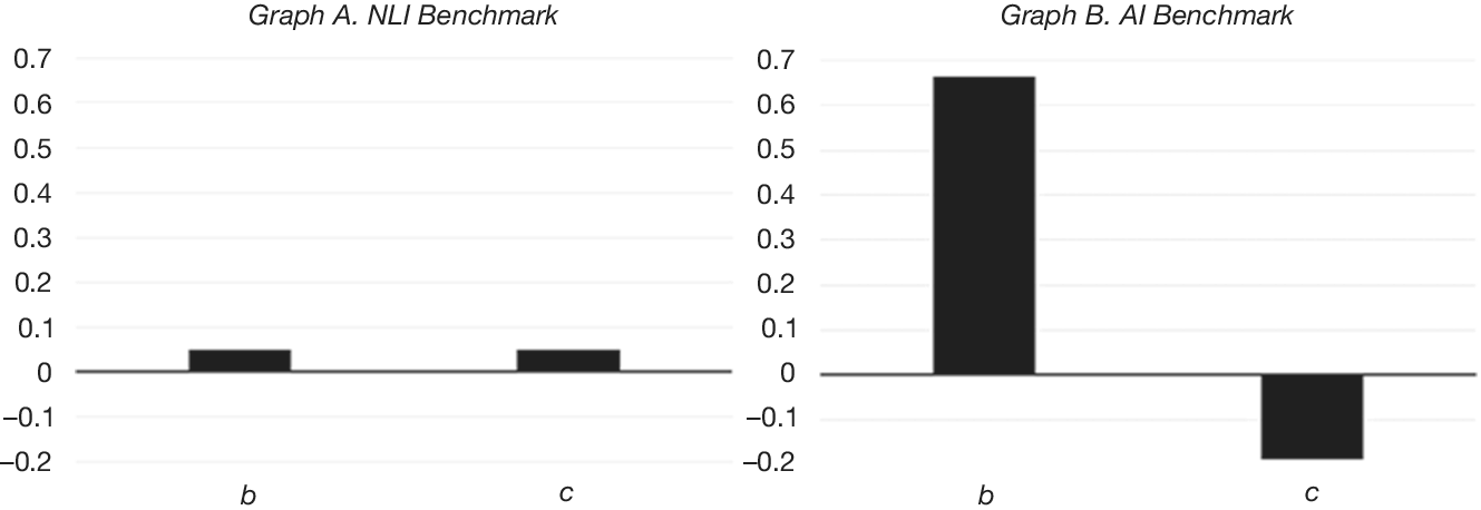
 and
$ c $
 in equation (9)), we solve the model numerically. Figure 1 presents the values of coefficients
$ b $
 and
$ c $
 as predicted by the two benchmarks for
$ {\sigma}_v^2/{\sigma}_u^2=1 $
 ,
$ {\sigma}_v^2/{\sigma}_w^2=1 $
 and
$ n=3 $
 .Footnote
9
Figure 1 plots the values of sensitivity coefficients
$ b $
 and
$ c $
 of future returns
$ {r}_{1,3} $
 on insider’s and informed traders’ demands
$ {\zeta}_1 $
 and
$ {\xi}_1 $
 , respectively. The coefficients are computed based on the multivariate regression
$ {r}_{1,3}={b}_0+b{\zeta}_1+c{\xi}_1+\unicode{x025B} $
 . Graph A corresponds to the
$ NLI $
 benchmark of the model and Graph B corresponds to the
$ AI $
 benchmark. The primitive parameters are:
$ {\sigma}_v^2/{\sigma}_u^2={\sigma}_v^2/{\sigma}_w^2=1 $
 and
$ n=3 $
 . The remaining parameters are computed numerically by solving the system of equations (6) and (8) for the
$ NLI $
 and
$ AI $
 benchmark, respectively.

Figure 1 Long description
A two-panel bar chart. Both panels share a y-axis ranging from negative 0.2 to 0.7 with increments of 0.1. The x-axis for both panels contains two categories: b and c.
Graph A, titled N L I Benchmark, shows two small positive bars of equal height. Bar b and bar c both reach approximately 0.05 on the y-axis.
Graph B, titled A I Benchmark, shows much larger values with opposing directions. Bar b is a tall positive bar reaching approximately 0.65. Bar c is a negative bar extending downward to approximately negative 0.2.
In the
$ NLI $
 benchmark, both types of informed traders use only the short-term information
$ {v}_1 $
 , which positively correlates with the long-term fundamental value
$ {v}_0+{v}_1+{v}_2 $
 . This means that the demands of both types of traders positively predict future stock returns. If insiders trade also on the long-term information
$ {v}_2 $
 , as in the
$ AI $
 benchmark, arbitrageurs are able to predict future returns relatively less well, and therefore the coefficient
$ c $
 is negative. When both
$ {v}_1 $
 and
$ {v}_2 $
 are either positive or negative, the arbitrageurs’ prediction has a correct sign. However, when
$ {v}_1 $
 and
$ {v}_2 $
 have opposite signs, arbitrageurs’ demands and future returns are negatively correlated. On average, the negative correlation in the latter case dominates the positive correlation in the former case, and the overall effect, as reflected in the coefficient
$ c $
 , is negative. In summary, our first hypothesis highlights the relative informational advantage of the insider over arbitrageurs. We formulate a null hypothesis and two alternative hypotheses corresponding to the two benchmarks.
Hypothesis 10. (relative predictive power of informed trading). Arbitrageurs’ demand conditional on insider’s demand does not predict future return.
Hypothesis 1NLI. Arbitrageurs’ demand conditional on insider’s demand predicts positive future return.
Hypothesis 1AI. Arbitrageurs’ demand conditional on insider’s demand predicts negative future return.
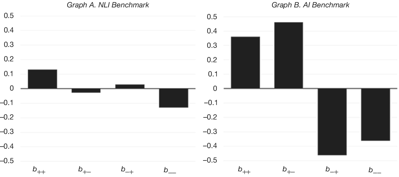
Figure 2 provides predictions for categorical rather than continuous demand variables as reflected in equation (10)), assuming
$ {\sigma}_v^2/{\sigma}_u^2=1 $
 ,
$ {\sigma}_v^2/{\sigma}_w^2=1 $
 , and
$ n=3 $
 . We consider separately demand sensitivities when the insider and arbitrageurs both buy or sell (
$ {b}_{++} $
 and
$ {b}_{--} $
 ) versus when their demands have opposite signs (
$ {b}_{+-} $
 and
$ {b}_{-+} $
 ).
Figure 2 plots the expectations of future returns
$ {r}_{1,3} $
 conditional on signs of order flow variables
$ {\zeta}_1 $
 and
$ {\xi}_1 $
 . Coefficient
$ {b}_{++} $
 ,
$ {b}_{+-} $
 ,
$ {b}_{-+} $
 and
$ {b}_{--} $
 are computed based on the multivariate regression
$ {r}_{1,3}={b}_{++}{\unicode{x1D540}}_{\zeta_1>0,{\xi}_1>0}+{b}_{+-}{\unicode{x1D540}}_{\zeta_1>0,{\xi}_1<0}+{b}_{-+}{\unicode{x1D540}}_{\zeta_1<0,{\xi}_1>0}+{b}_{--}{\unicode{x1D540}}_{\zeta_1<0,{\xi}_1<0}+\unicode{x025B} $
 . The primitive parameters are:
$ {\sigma}_v^2/{\sigma}_u^2={\sigma}_v^2/{\sigma}_w^2=1 $
 and
$ n=3 $
 . The remaining parameters are computed numerically by solving the system of equations (6) and (8) for the
$ NLI $
 and
$ AI $
 benchmark.

Figure 2 Long description
The image consists of two side-by-side bar charts. Both charts share a Y-axis ranging from negative 0.5 to 0.5 with increments of 0.1. The X-axis for both charts lists four variables: b sub plus plus, b sub plus minus, b sub minus plus, and b sub minus minus.
Graph A, titled N L I Benchmark, shows relatively low magnitude coefficients. The first bar, b sub plus plus, is positive at approximately 0.13. The second bar, b sub plus minus, is slightly negative at approximately negative 0.03. The third bar, b sub minus plus, is slightly positive at approximately 0.03. The fourth bar, b sub minus minus, is negative at approximately negative 0.13.
Graph B, titled A I Benchmark, shows significantly higher magnitude coefficients. The first bar, b sub plus plus, is positive at approximately 0.36. The second bar, b sub plus minus, is positive at approximately 0.46. The third bar, b sub minus plus, is strongly negative at approximately negative 0.46. The fourth bar, b sub minus minus, is negative at approximately negative 0.36.
Both benchmarks imply that whenever insider’s and arbitrageurs’ demands have the same sign, demands of the two types correctly forecast the future return:
$ {b}_{++} $
 is positive and
$ {b}_{--} $
 is negative. However, in the case of opposite signs of insider’s and arbitrageurs’ demands, the
$ NLI $
 benchmark predicts that the expected future stock return is positive whenever the arbitrageurs’ aggregate demand is positive and vice versa:
$ {b}_{-+} $
 is positive, while
$ {b}_{+-} $
 is negative. The higher predictive power of arbitrageurs’ demand stems from the fact that their demands are aggregated over
$ n $
 arbitrageurs and the noise in the arbitrageurs’ demands, which is due to independent shocks to their initial endowments, is diversified away. The
$ AI $
 benchmark in the case of opposite signs of insider’s and arbitrageurs’ demands predicts that the expected future stock return is positive whenever the insider’s demand is positive because the insider is informed about the long-term innovation to the fundamental value, while arbitrageurs are not. This implies that
$ {b}_{+-} $
 is positive, while
$ {b}_{-+} $
 is negative. As a result, Hypothesis 2 concerns the predictive ability of informed demands when the two types of informed traders disagree on the direction of trading.
Hypothesis 20. (predictive ability of disagreement between the two types of informed traders). When demands of the insider and arbitrageurs have opposite signs, the demands of neither type of informed traders predict future returns.
Hypothesis 2NLI. Conditional on demands of the insider and arbitrageurs having opposite signs, the future return is positive whenever arbitrageurs buy and negative whenever they sell.
Hypothesis 2AI. Conditional on demands of the insider and arbitrageurs having opposite signs, the future return is positive whenever the insider buys and negative whenever he/she sells.
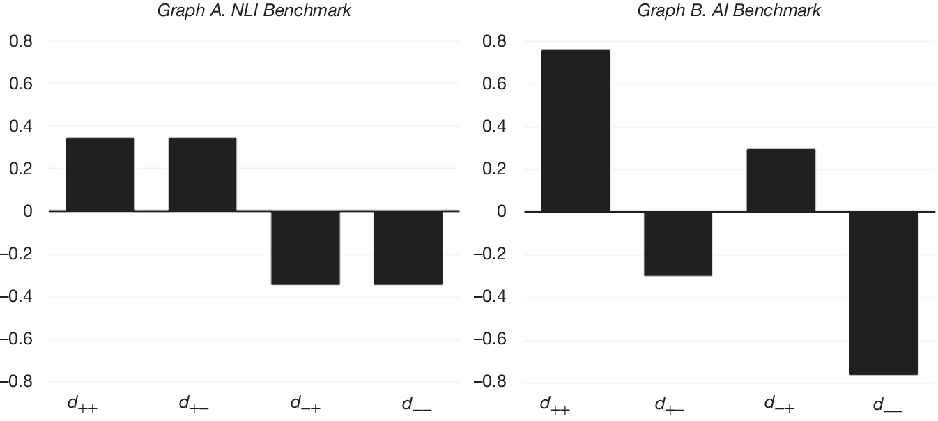
Hypothesis 3 is somewhat different. It does not concern return-demand sensitivities but focuses on the relationship between the insider’s demand and the short-term and long-term information. Estimation of the direct sensitivity of insider’s demand to the two types of information complements Hypothesis 2. Figure 3 presents the model’s predicted sensitivities to information as represented by coefficients
$ {d}_{++} $
 to
$ {d}_{--} $
 in equation (11). We again differentiate the
$ NLI $
 and
$ AI $
 benchmarks and assume
$ {\sigma}_v^2/{\sigma}_u^2=1 $
 ,
$ {\sigma}_v^2/{\sigma}_w^2=1 $
 and
$ n=3 $
 .
Figure 3 plots the conditional expectations of insider’s demand
$ {\zeta}_1 $
 conditional on signs of fundamental innovations
$ {v}_1 $
 and
$ {v}_2 $
 . The primitive parameters are:
$ {\sigma}_v^2/{\sigma}_u^2={\sigma}_v^2/{\sigma}_w^2=1 $
 and
$ n=3 $
 . The remaining parameters are computed numerically by solving the system of equations (6) and (8) for the
$ NLI $
 and
$ AI $
 benchmark.

Figure 3 Long description
The image consists of two side-by-side bar graphs, Graph A and Graph B. Both graphs share a y-axis ranging from negative 0.8 to 0.8 with increments of 0.2 and an x-axis with four categories: d sub plus plus, d sub plus minus, d sub minus plus, and d sub minus minus.
Graph A. N L I Benchmark:
* d sub plus plus: Positive bar at approximately 0.35.
* d sub plus minus: Positive bar at approximately 0.35.
* d sub minus plus: Negative bar at approximately negative 0.35.
* d sub minus minus: Negative bar at approximately negative 0.35.
Graph B. A I Benchmark:
* d sub plus plus: Positive bar at approximately 0.75.
* d sub plus minus: Negative bar at approximately negative 0.3.
* d sub minus plus: Positive bar at approximately 0.3.
* d sub minus minus: Negative bar at approximately negative 0.75.
The
$ NLI $
 benchmark implies that the insider’s demand is positive only when the short-term information
$ {v}_1 $
 is positive. This happens because the insider does not use the long-term information
$ {v}_2 $
 and hence buys only when
$ {v}_1 $
 signal commands so. In the
$ AI $
 benchmark, the insider optimally forms a positive demand whenever the long-term information
$ {v}_2 $
 is positive, anticipating a positive future return. In the case of
$ {v}_1<0 $
 and
$ {v}_2>0 $
 (
$ {v}_1>0 $
 and
$ {v}_2<0 $
 ), the fundamental asset value is on average zero. However, the insider buys (sells) to exploit the selling (buying) pressure coming from arbitrageurs who act on the basis of
$ {v}_1 $
 only. As a result, insider’s demand is contrarian to the short-term information when the short-term and long-term signals are of opposite signs.
Hypothesis 30. (relationship between insider’s demand and long-term information). Conditional on the short-term and long-term information having opposite signs, the insider’s demand is sensitive to neither the short-term nor long-term information.
Hypothesis 3NLI. Conditional on the short-term and long-term information having opposite signs, the insider tends to sell when the short-term information is negative and buy when the short-term information is positive (the insider’s demand is not sensitive to the long-term information).
Hypothesis 3AI. Conditional on the short-term and long-term information having opposite signs, the insider tends to sell when the long-term information is negative and buy when it is positive.
Overall, our hypotheses aim to establish whether insider’s trading strategies take into account the short-term and/or long-term information. The main identification strategy is comparing his/her demand to the demand of traders who use only the short-term information. Using short-sellers’ demand to proxy for arbitrageurs’ trades, we are able to estimate the sensitivity of insider trades to the short-term versus long-term information.
III. Data
Our sample comprises firm-quarter information from July 2006 to December 2017 for 6,046 publicly listed U.S. firms. We consider all U.S. common stocks that are traded on the NYSE, NASDAQ, or AMEX exchanges.Footnote 10 We obtain quarterly earnings announcements from the Compustat quarterly data file and delete firm-quarters for which this data is unavailable. Compustat is also the source of accounting information. Insider trading data comes from Thomson Financial Insider Filings that contain all insider trading activity as reported in Forms 3, 4, and 5 specified in the Securities Exchange Act of 1934. The data set contains detailed information about all reported transactions, including the trading date, reporting date, insider name, insider’s position in their firm, number of shares traded, transaction price, and transaction type (purchase or sale). We consider only open-market purchases and sales by officers and directors.Footnote 11 As insiders sometimes trade several times on the same day, we sum all insider transactions by the same director in the same direction (purchases/sales) within 1 day, but keep transactions if they are in different directions even on the same day. Data on short selling and equity-lending supply is from Markit (which acquired Data Explorers).Footnote 12 The data on insider trading and short selling around earnings announcements is matched with stock-return data from CRSP, and analyst forecast data from IBES.
The number of shares sold and bought by insiders and the daily number of stocks on loan based on shorting transactions that are initiated on the most recent business day should reflect informed trading as defined in our model in Section II. For insider trading, we define net insider selling (
$ {nis}_{kt} $
 ) as the difference between the number of shares sold and bought on a given day
$ t $
 by all insiders of a focus firm
$ k $
 , scaled by the number of shares outstanding. To distinguish net sales from net purchases, we also define
$ {nispos}_{kt} $
 where we replace all negative values with zeros and keep all positive values—this variable represents insider sales that are larger than insider purchases. Similarly, we define
$ {nisneg}_{kt} $
 by keeping negative values of
$ {nis}_{kt} $
 and then taking an absolute value for easier interpretation. This variable then represents insider purchases that exceed insider sales. Short selling (
$ {relss}_{kt} $
 ) is measured as the number of stocks on loan based on shorting transactions of the focus firm
$ k $
 that are initiated on the day
$ t $
 , scaled by the number of shares outstanding.
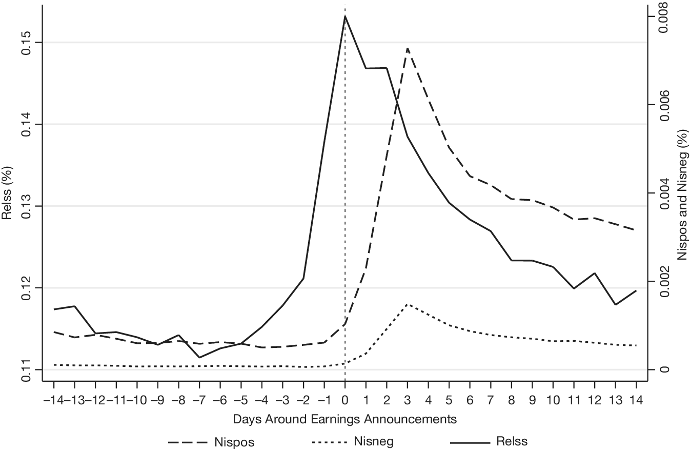
Figure 4 plots averages for the relative short-selling volume
$ {relss}_t $
 , the net insider selling
$ {nispos}_t $
 , and the net insider buying
$ {nisneg}_t $
 29 days around earnings announcements. As the magnitude of insider trades is considerably smaller than the magnitude of short sales, we place the range of values for shorting transactions on the left axis and of insiders’ transactions on the right axis. We can see that earnings announcements have a significant effect on the trading patterns of both types of informed traders. In line with Engelberg et al. (Reference Engelberg, Reed and Ringgenberg2012), short sales increase sharply at day
$ -1 $
 and gradually decrease afterward. Insider sales peak at day +3 and their trading on day +14 is still markedly higher compared to the pre-announcement level, which is not the case for short sales. It is apparent that short sellers are faster than insiders—their trades peak immediately on the announcement day, while insiders follow only 3 days later for both insider sales and purchases. This insider trading lag is most likely due to restrictive “blackout” periods imposed on insiders by their employers in order to minimize their information advantage.Footnote
13 The short sales decrease smoothly since day +2 and do not seem to respond to the peak in insider trading.
Figure 4 plots the averages of daily positive net insider selling (
$ {nispos}_t $
 , dashed line), negative net insider selling (
$ {nisneg}_t $
 , dotted line) together with the relative number of shares shorted (
$ {relss}_t $
 , solid line) 14 day before and after earnings announcements. All shares traded are scaled by the number of shares outstanding and expressed in basis points. All variables are defined in Appendix A.

Figure 4 Long description
A line graph with two Y-axes and one X-axis. The X-axis represents Days Around Earnings Announcements, ranging from negative 14 to positive 14, with a vertical dotted line at day 0. The left Y-axis is labeled R E L S S percentage, ranging from 0.11 to 0.15. The right Y-axis is labeled N I S P O S and N I S N E G percentage, ranging from 0 to 0.008.
* The solid line (R E L S S) remains relatively flat around 0.115 until day negative 4, where it rises sharply to a peak of approximately 0.153 at day 0, then declines steadily back toward 0.12 by day 14.
* The dashed line (N I S P O S) remains flat near 0.001 until day 0, then spikes sharply to a peak of approximately 0.007 at day 3, followed by a gradual decline to 0.0035 by day 14.
* The dotted line (N I S N E G) remains near 0 until day 0, shows a small peak of approximately 0.0015 at day 3, and then levels off slightly above 0.001 through day 14.
As our analysis centers around earnings announcements and focuses on the ability of informed traders to interpret public information, we need to aggregate insider and short-selling activity following quarterly earnings announcements. We consider a “response window” of (0,+5) to reflect that informed trading should be prompt, and we want to exclude the possibility of short sellers following insider trades. This could potentially happen only after 5 days from an earnings announcement; 3 days due to insider trading bans plus 2 days of reporting lag, on average. Consequently, we compute the average daily net insider sales (
$ nis $
 ), positive net insider sales (
$ nispos $
 ), and negative net insider sales (
$ nisneg $
 ) within the response window. Similarly, we compute the average daily relative number of shares on loan (
$ relss $
 ) within the 6 days. We define the buy-and-hold stock return
$ {aret}_{k,t+5,t+6+h} $
 for firm
$ k $
 from day
$ t+5 $
 to day
$ t+6+h $
 after the earnings announcement date
$ t $
 adjusted for the corresponding
$ 5\times 5 $
 size and book-to-market portfolio return.Footnote
14
Table 1 shows firm-quarter summary statistics for all variables of interest that are defined in Appendix A. Panel A focuses on informed-trading variables over the
$ \left(0,+5\right) $
 response window, which are (except dummy variables) reported in basis points. The average daily net insider sales are only 0.6 bps of their shares outstanding per day during the 6 days. The average positive and negative values for net insider sales are 0.79 bps and 0.19 bps, respectively, which indicates that insiders, on average, sell more than they buy. The quartile statistics show that both net insider sales and purchases are quite rare. In contrast, short sellers are significantly more active. The average relative fraction of shares shorted is 14 bps per day. Only 25% of firm-quarters have an average daily number of shares shorted during the (0,+5) response window smaller than 1.67 bps.

Table 1 Long description
The table contains nine columns: Variable, Number of Observations, Mean, Standard Deviation, p 5, p 25, p 50, p 75, and p 95.
Panel A. Informed Trading over the (0, +5) Response Window:
* n i s: Mean 0.60, Std. Dev. 3.08, p 50 0.00.
* n i s p o s: Mean 0.79, Std. Dev. 2.86, p 50 0.00.
* n i s n e g: Mean 0.19, Std. Dev. 0.99, p 50 0.00.
* r e l s s: Mean 14.01, Std. Dev. 19.47, p 50 6.73.
* i s: Mean 0.19, Std. Dev. 0.38, p 50 0.00.
* i p: Mean 0.07, Std. Dev. 0.26, p 50 0.00.
Panel B. Future Returns (all values in percentages):
* a r e t sub t+5, t+26: Mean -0.58, Std. Dev. 10.25, p 50 -0.77.
* a r e t sub t+5, t+46: Mean -0.85, Std. Dev. 14.42, p 50 -1.15.
* a r e t sub t+5, t+66: Mean -0.84, Std. Dev. 18.06, p 50 -1.32.
* a r e t sub t+5, t+136: Mean -1.91, Std. Dev. 27.23, p 50 -2.78.
* a r e t sub t+5, t+256: Mean -2.82, Std. Dev. 32.23, p 50 -3.88.
Panel C. Control Variables:
* Delta e p s: Mean -0.37 percent, Std. Dev. 6.99 percent.
* e a a r: Mean 0.16 percent, Std. Dev. 6.93 percent.
* p a s t r e t: Mean -2.22 percent, Std. Dev. 32.55 percent.
* Delta e a r n sub t+q1: Mean 0.001, Std. Dev. 0.035.
* Delta e a r n sub t+q3: Mean 0.001, Std. Dev. 0.039.
* Delta e a r n sub t+q4: Mean 0.001, Std. Dev. 0.039.
* e a a r sub t+q1: Mean -0.005, Std. Dev. 0.364.
* e a a r sub t+q3: Mean -0.008, Std. Dev. 0.401.
* e a a r sub t+q4: Mean -0.008, Std. Dev. 0.409.
All variables in Panel A and B have 132,240 observations. Panel C observations range from 115,997 to 132,240.
In order to test our hypotheses, we distinguish intensive informed trading using a set of dummy variables. First, we set intensive insider selling (
$ {is}_{k,t,t+5} $
 ) and buying (
$ {ip}_{k,t,t+5} $
 ) dummies to 1 when net insider selling is positive and negative, respectively, over the
$ \left(0,+5\right) $
 response window. Accordingly, the dummy
$ {noit}_{k,t,t+5} $
 for “no insider trading” is set to 1 when net insider selling is equal to 0 over the response window.Footnote
15 Finally, we define firm-quarters with intensive short selling (
$ {ssh}_{k,t,t+5} $
 ) as quarters with the relative number of shares shorted being in the top quintile and firm-quarters with low-intensity short selling (
$ {ssl}_{k,t,t+5} $
 ) as quarters with the relative number of shares shorted being in the bottom quintile. The dummy variable
$ {ssm}_{k,t,t+5} $
 corresponds to the 3 middle quintiles of short selling. To preserve space, we simplify notation for these variables and use
$ is $
 ,
$ ip $
 ,
$ noit $
 ,
$ ssh $
 ,
$ ssm $
 , and
$ ssl $
 in all tables and
$ {is}_{kt} $
 , …,
$ {ssl}_{kt} $
 in equations. The average values for
$ is $
 and
$ ip $
 in Panel A of Table 1 show that only about 19% of all firm-quarters experience net insider selling and about 7% experience net insider buying over the
$ \left(0,+5\right) $
 response window. No insider trading is the complement to these two groups. Statistics for
$ ssh $
 ,
$ ssm $
 , and
$ ssl $
 are self-explanatory and therefore not tabulated.
Panels B and C of Table 1 show summary statistics for future returns and control variables, respectively. The average size- and book-to-market-adjusted return over the 20 business days just after the
$ \left(0,+5\right) $
 response window is
$ -0.58\% $
 and returns deteriorate further over longer horizons. The negative values are due to the size and book-to-market adjustments as the market-adjusted model shows future returns with positive values.Footnote
16 The average firm in our sample has a negative change in earnings per share relative to 4 quarters back of −0.37%. Nevertheless, the average market reaction to the earnings announcement is 0.16%. The past 1-year return, again with the size and book-to-market adjustment, is −2.22%. The two measures to determine the direction of the long-term information used for testing Hypothesis 3 are based on future-quarter earnings innovations and are discussed in more detail in Section IV. The first measure
$ \Delta earn $
 takes the change in net income scaled by total assets in thousands, while the second measure
$ eaar $
 focuses on the 3-day market reaction to future earnings announcements, again size and book-to-market adjusted. Median values for both measures are close to 0, but they both exhibit large variation.
Table 2 provides statistics for interaction terms between intensive insider and short-selling activity during the 6-day response window. Insiders and short sellers sell together relatively frequently. The first set of interaction terms between insider selling and the three categories of short selling shows that insiders are net selling in about 17.7% of all quarters (
$ is $
 in column 2). In 4.7% of all quarters, they net sell together with intensive short selling (
$ is\times ssh $
 ), while in only 0.9% of all quarters, they net sell when the short-selling activity is very low (
$ is\times ssl $
 ). The insider tendency to trade when short selling is high pertains also when considering the fraction of shares traded (5.18 bps in column 5) or the average trade dollar value ($2.6 million in column 7). The corresponding numbers for low short-selling intensity are 4.56 bps and $1.3 million, respectively.

Table 2 Long description
The table consists of 14 rows and 8 numbered columns.
Columns are:
1. Number of Quarters.
2. Percentage of All Quarters.
3. Within-Group Fraction.
4. r e l s s.
5. n i s p o s.
6. n i s n e g.
7. Total Sale Value.
8. Total Purchase Value.
Rows by Category:
- i s times s s h: 6,161 quarters, 4.66 percent, 26.29 percent within-group, r e l s s 45.51, n i s p o s 5.18, n i s n e g 0, Sale Value $2,628,562, Purchase Value $6,079.
- i s times s s m: 16,099 quarters, 12.17 percent, 68.69 percent within-group, r e l s s 9.46, n i s p o s 4.16, n i s n e g 0, Sale Value $2,266,129, Purchase Value $5,667.
- i s times s s l: 1,178 quarters, 0.89 percent, 5.03 percent within-group, r e l s s 0.42, n i s p o s 4.56, n i s n e g 0, Sale Value $1,316,619, Purchase Value $4,790.
- i s (Subtotal): 23,438 quarters, 17.72 percent.
- i p times s s h: 2,187 quarters, 1.65 percent, 22.43 percent within-group, r e l s s 48.96, n i s p o s 0, n i s n e g 2.58, Sale Value $18,356, Purchase Value $420,448.
- i p times s s m: 5,531 quarters, 4.18 percent, 56.72 percent within-group, r e l s s 8.42, n i s p o s 0, n i s n e g 2.39, Sale Value $11,903, Purchase Value $219,085.
- i p times s s l: 2,034 quarters, 1.54 percent, 20.86 percent within-group, r e l s s 0.29, n i s p o s 0, n i s n e g 3.12, Sale Value $1,267, Purchase Value $72,369.
- i p (Subtotal): 9,752 quarters, 7.37 percent.
- n o i t times s s h: 17,251 quarters, 13.05 percent, 17.42 percent within-group, r e l s s 45.49, n i s p o s 0, n i s n e g 0.
- n o i t times s s m: 60,000 quarters, 45.37 percent, 60.58 percent within-group, r e l s s 7.90, n i s p o s 0, n i s n e g 0.
- n o i t times s s l: 21,799 quarters, 16.48 percent, 22.01 percent within-group, r e l s s 0.29, n i s p o s 0, n i s n e g 0.
- n o i t (Subtotal): 99,050 quarters, 74.90 percent.
- Total: 132,240 quarters, 100 percent.
- Unconditional average: r e l s s 14.01, n i s p o s 0.79, n i s n e g 0.19, Sale Value $1,637,135, Purchase Value $72,697.
Net insider purchases are present in only 7.4% of quarters (
$ ip $
 in column 2) and are equally likely with low and high short-selling activity. Column 6 shows that insiders buy significantly more (3.12 bps of shares outstanding) in low short-selling activity quarters than in high short-selling activity quarters (2.58 bps). However, the average dollar value purchased is at $0.4 million, almost 6-fold higher in the high than in the low sort selling category (column 8).
Finally, short selling without any insider trading activity covers 74.9% of all quarters (
$ noit $
 in column 2). The intensity of short selling without any presence of insider trading activity inclines toward lower levels. The fraction of quarters with high short selling and without any insider trading activity is 13.05% (
$ noit\times ssh $
 in column 2). This represents 17% of all quarters without any insider trading activity (
$ noit\times ssh $
 in column 3) and is significantly lower than the unconditional fraction of 20% at the 1% level.Footnote
17 Moreover, low short-selling activity without any insider trading activity is reported in 16.5% of all quarters (
$ noit\times ssl $
 in column 2). This represents 22% of quarters without insider trading and is significantly higher than 20%, indicating again that short sellers are less active when insiders are not trading.
The last row in columns 5 to 8 shows that insider sales are substantially larger than purchases both by the fraction of shares traded and dollar trade value. Insiders on average sell $1.6 million (about 0.79 bps of shares outstanding) but buy only $0.07 million (0.19 bps of shares outstanding). The average sale value during quarters of high short selling is $2.6 million, and the average purchase value during quarters of low short selling is only $0.07 million.
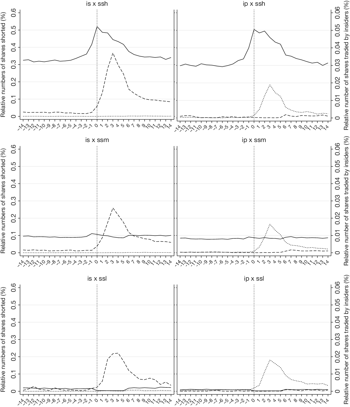
Figure 5 shows that the two types of informed traders sell indeed more when selling together. We graph the selling activity for 29 days around earnings announcements as in Figure 4 but now conditional on the set of informed-trading interaction categories used in Table 2 within the (0,+5) response window, not showing plots when insiders are not trading. Short-selling peaks at day 0 regardless of the direction of insider trading. Still, short sellers’ trades peak higher when insiders sell rather than buy. Similarly, insider sales (purchases) peak at day +3 regardless of short-sellers’ trading. The peak is sharper when insiders sell together with high short selling, but surprisingly, it seems to be sharper also with purchases when insiders and short sellers disagree.
Figure 5 plots the averages of daily positive net insider selling (
$ {nispos}_t $
 , dashed line) and negative net insider selling (
$ {nisneg}_t $
 , dotted line) together with the relative number of shares shorted (
$ {relss}_t $
 , solid line) 14-day before and after earnings announcements by six interaction categories between insider and short-selling activity. The dummies for informed trading activity
$ is $
 ,
$ ip $
 ,
$ ssh $
 ,
$ ssm $
 , and
$ ssl $
 are defined based on the (0,+5) response window. All shares traded are scaled by the number of shares outstanding and expressed in basis points. All variables are defined in Appendix A.

Figure 5 Long description
A grid of six line graphs. Each graph shares a common x-axis representing days relative to an earnings announcement, ranging from negative 14 to positive 14, with a vertical dashed line at day 0. The left y-axis measures Relative numbers of shares shorted (%) from 0 to 0.6. The right y-axis measures Relative number of shares traded by insiders (%) from 0 to 0.06.
Three line types are used: a solid line for relative shares shorted, a dashed line for positive net insider selling, and a dotted line for negative net insider selling.
* Top-Left (i s x s s h): The solid line peaks sharply at day 0 near 0.5. The dashed line shows a significant peak around day 3, reaching approximately 0.35.
* Top-Right (i p x s s h): The solid line peaks at day 0 near 0.5. The dotted line shows a moderate peak around day 3, reaching approximately 0.02.
* Middle-Left (i s x s s m): The solid line remains flat near 0.1. The dashed line peaks around day 3 at approximately 0.25.
* Middle-Right (i p x s s m): The solid line remains flat near 0.1. The dotted line peaks around day 3 at approximately 0.015.
* Bottom-Left (i s x s s l): The solid line is very low, near 0.02. The dashed line peaks around day 3 at approximately 0.22.
* Bottom-Right (i p x s s l): The solid line is very low, near 0.01. The dotted line peaks around day 3 at approximately 0.018.
IV. Empirical Results
A. Predictability of Future Returns
To test Hypothesis 1 on the relative predictive power of informed trading, we regress future returns on insider-trading and short-selling intensity dummies simultaneously:

where
$ {aret}_{k,t+5,t+6+h} $
 denotes abnormal return in stock
$ k $
 from
$ t+5 $
 to
$ t+6+h $
 relatively to the earnings announcement at
$ t $
 , with
$ h\in \left\{\mathrm{20,40,60,130,250}\right\} $
 ;
$ {is}_{kt} $
 and
$ {ip}_{kt} $
 denote dummy variables for intensive net insider sales and purchases, respectively, in firm
$ k $
 over the
$ \left(0,+5\right) $
 response window relatively to
$ t $
 ; and
$ {ssh}_{kt} $
 and
$ {ssl}_{kt} $
 denote short selling in the highest and lowest quintiles, respectively, in firm
$ k $
 over the
$ \left(0,+5\right) $
 response window. Figure 6 shows the timings. Variables
$ {X}_{kt} $
 include firm-specific characteristics including the past 1-year return
$ {pastret}_{k,t-1y,t-2} $
 , the earnings announcement abnormal return
$ {eaar}_{k,t-2,t+1} $
 , the change in earnings-per-share
$ \Delta {eps}_{k,t-q4,t} $
 as well as firm and year fixed-effect dummies. Standard errors are clustered within firms.
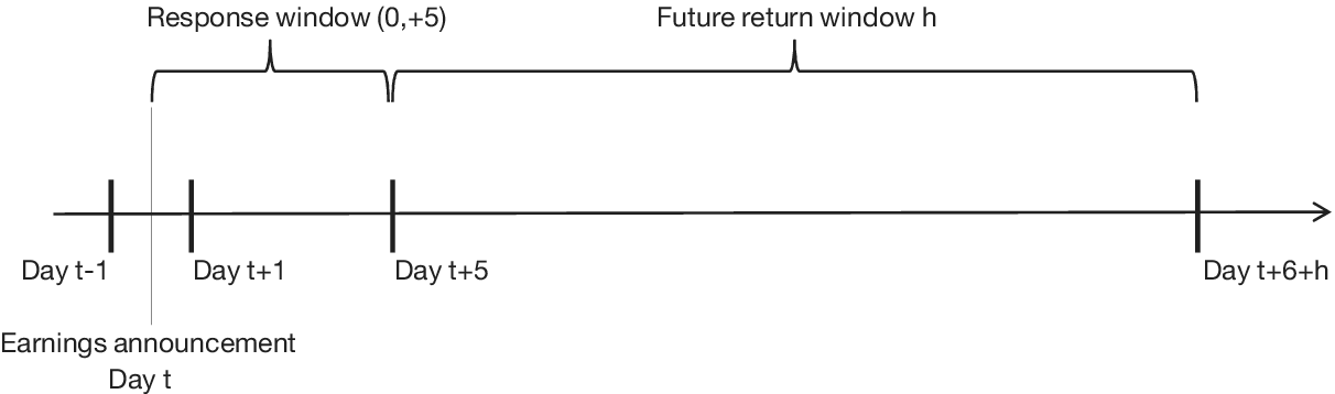
Figure 6 shows relative timings of informed trading during the response window and timings of future abnormal returns. Everything is arranged relatively to the earnings announcement that is set as day
$ t $
 . We take into account only trading days. Accordingly, we establish i) the earnings-announcement window, which starts on day
$ t-1 $
 and ends on day
$ t+1 $
 ; ii) the response window when insiders and short sellers trade, which starts on day
$ t $
 and ends on day
$ t+5 $
 ; and iii) the future-return window, which runs between days
$ t+5 $
 and
$ t+6+h $
 .

Hypothesis 1 highlights the relative informational advantage of insiders over short sellers in the
$ AI $
 benchmark. In particular, Hypothesis 1
AI
predicts that future returns are negatively correlated with short-sellers’ demand, which means that
$ {c}_1 $
 should be positive and
$ {c}_2 $
 negative. In contrast, Hypothesis 1
NLI
predicts negative
$ {c}_1 $
 and positive
$ {c}_2 $
 .
Table 3 shows the results with the first 2 columns summarizing Hypothesis 1 predictions. Future abnormal returns are significantly more negative for stocks with insider selling and significantly more positive for stocks with insider buying. Similarly, future abnormal returns are significantly more negative for intensively shorted stocks (except for the shortest horizon
$ h=20 $
 ) and significantly more positive for stocks with the lowest levels of short selling for all horizons.Footnote
18 This shows that both insiders’ and short-sellers’ demands predict future returns, which is in line with existing literature (Huddart et al. (Reference Huddart, Ke and Shi2007), Akbas et al. (Reference Akbas, Jiang and Koch2020)). More importantly, we reject the null hypothesis (Hypothesis 10) for all horizons
$ h $
 in favor of the alternative Hypothesis 1
NLI
. Coefficient
$ {c}_1 $
 is significantly negative and
$ {c}_2 $
 is significantly positive at the 1% level after controlling for insider trading, which provides initial evidence in favor of the
$ NLI $
 benchmark that insiders abstain from trading on the foreknowledge of future material information, but take advantage of short-term mispricing.

Table 3 Long description
The table consists of 8 columns and 11 rows. The header row includes columns for H 1 sub N L I, H 1 sub I S S, and time horizons h = 20, h = 40, h = 60, h = 130, and h = 250.
Row 1: i s. Values for h = 20 to h = 250 are -0.006***, -0.008***, -0.014***, -0.026***, and -0.031***.
Row 2: i p. Values for h = 20 to h = 250 are 0.015***, 0.016***, 0.021***, 0.034***, and 0.036***.
Row 3: s s h (c sub 1). H 1 sub N L I is c sub 1 < 0. H 1 sub I S S is c sub 1 > 0. Values for h = 20 to h = 250 are -0.001, -0.006***, -0.011***, -0.023***, and -0.029***.
Row 4: s s l (c sub 2). H 1 sub N L I is c sub 2 > 0. H 1 sub I S S is c sub 2 < 0. Values for h = 20 to h = 250 are 0.005***, 0.011***, 0.018***, 0.036***, and 0.046***.
Row 5: p a s t r e t. Values for h = 20 to h = 250 are -0.004***, -0.009***, -0.026***, -0.050***, and -0.072***.
Row 6: e a a r. Values for h = 20 to h = 250 are 0.046***, 0.071***, 0.050***, 0.042***, and 0.051***.
Row 7: Delta eps. Values for h = 20 to h = 250 are 0.033***, 0.024***, 0.022*, 0.001, and 0.005.
Row 8: Constant. Values for h = 20 to h = 250 are -0.106, -0.061, -0.095, -0.203, and -0.234.
Row 9: Nr. of obs. All values are 130,240.
Row 10: R-squared. Values for h = 20 to h = 250 are 0.71%, 0.92%, 1.11%, 1.83%, and 1.99%.
To test Hypothesis 2 concerning the predictive power of a disagreement between the two types of informed traders, we interact insiders’ and short sellers’ intensive trading dummies:

where matrix
$ {X}_{kt} $
 contains the same control variables as in model (12), but we add interaction terms for the no insider trading dummy
$ noit $
 and the middle short-selling quintiles dummy
$ ssm $
 . The regression constant reflects the remaining category of quarters
$ ssm\times noit $
 . As we focus on the predictive power of the two informed traders’ demands when they are in disagreement, Hypothesis 2
NLI
suggests a higher predictive power for short-sellers’ demands:
$ {b}_{+-} $
 should be negative and
$ {b}_{-+} $
 positive. Hypothesis 2
AI
predicts the opposite signs as insiders’ predictive power is higher when they use foreknowledge of future material information.
Panel A of Table 4 shows the results with the first 2 columns summarizing Hypothesis 2 predictions. We reject the null Hypothesis 2
0
at all horizons
$ h $
 , but this time it is rejected in favor of Hypothesis 2
NLI
or Hypothesis 2
AI
, depending on whether insiders buy or sell. Specifically, the coefficient
$ {b}_{+-} $
 corresponding to the interaction term
$ ip\times ssh $
 (insiders are buying while short sellers are selling intensively) is positive and statistically significant for all horizons. This means that when insiders and short sellers disagree and insiders buy, future returns are positive—insiders predict future returns better than short sellers. Hence, insiders’ demand is based on foreknowledge of future material information. The null Hypothesis 2
0
is rejected in favor of the alternative Hypothesis 2
AI
for insider purchases. It is noteworthy that this result applies under the assumption that short sellers are as good as insiders in processing the short-term public information. Section VI discusses alternative scenarios.

Table 4 Long description
The table is divided into two main sections: Panel A and Panel B.
Header Row: The columns represent different time horizons or hypotheses, labeled H 2 sub N L I, H 2 sub I, h = 20, h = 40, h = 60, h = 130, and h = 250.
Panel A: Predictive Regression of Disagreement Among Traders on Future Returns.
* i p times s s l (b sub plus plus): Values increase from 0.020 at h = 20 to 0.063 at h = 250.
* i p times s s h (b sub plus minus): Values range from 0.016 at h = 20 to 0.018 at h = 250.
* i s times s s l (b sub minus plus): Values range from -0.001 at h = 20 to 0.015 at h = 250.
* i s times s s h (b sub minus minus): Values decrease from -0.007 at h = 20 to -0.064 at h = 250.
* Additional rows include i p times s s m, i s times s s m, n o i t times s s l, n o i t times s s h, p a s t r e t, e a a r, Delta e p s, Constant, Number of observations (132,240 for all), and R-squared (increasing from 0.70% to 1.99%).
Panel B: Net Dollar Profits per Trade.
* i p times s s l: Ranges from -$172 at h = 20 to $1,614 at h = 250.
* i p times s s m: Ranges from -$433 at h = 20 to $1,243 at h = 250.
* i p times s s h: Ranges from -$1,163 at h = 20 to $2,430 at h = 250.
* i s times s s l: Ranges from $2,683 at h = 20 to $1,268 at h = 250.
* i s times s s m: Increases significantly from $4,671 at h = 20 to $28,727 at h = 250.
* i s times s s h: Increases significantly from $5,391 at h = 20 to $48,105 at h = 250.
Statistical significance is indicated by asterisks, with three asterisks representing the highest level of significance.
In contrast, the coefficient
$ {b}_{-+} $
 for the interaction term
$ is\times ssl $
 (insiders are selling while short sellers are “buying”) is positive for
$ h\ge 40 $
 and significant for
$ h=40 $
 . This means that when demands of insiders and short sellers have opposite signs and insiders sell, future returns are positive—insiders do not predict future returns well. Insider selling is not based on foreknowledge of future material information. In the case of insider sales, the null Hypothesis 2
0
is rejected in favor of the alternative Hypothesis 2
NLI
.
Overall, Panel A suggests that when insiders and short sellers disagree in their trading, insiders tend to abstain from selling on foreknowledge of future material information. Also, insiders’ sales forecast future returns when their demand is aligned with short-sellers’ demand; they effectively hide behind the high short-sellers’ demand. In contrast, insiders are sometimes able to take advantage of foreknowledge of future material information when buying. As shareholders are usually more determined to sue when suffering from negative returns, the differing pattern across purchases and sales minimizes insiders’ chances of legal jeopardy in the future (Ke et al. (Reference Ke, Huddart and Petroni2003), Cheng and Lo (Reference Cheng and Lo2006), Kallunki, Kallunki, Nilsson, and Puhakka (Reference Kallunki, Kallunki, Nilsson and Puhakka2018)).
Still, it is important to check whether insiders are able to earn significant dollar amounts during periods of their agreement or disagreement with short sellers, as positive correlation between trades and future returns is not necessarily translated into significant dollar profits for insiders (Cziraki and Gider (Reference Cziraki and Gider2021)). This is due to variation in trading volumes that differ significantly across different categories, as we show in Table 1, but also across different percentage returns. We calculate the dollar profit for each trade within the (0,+5) response window as the inflation-adjusted dollar value expressed in 2017 U.S. dollars and multiplied by the buy-and-hold abnormal return over the corresponding time horizon, which is size and book-to-market adjusted. In order to express profits with positive values, we multiply the resulting number for sales by
$ -1 $
 . For each firm-quarter, we average over all trades that fall within the (0,+5) response window.
Panel B of Table 4 shows averages of dollar profits per trade across different trading categories and horizons.Footnote
19 The unconditional average dollar profit per trade in our sample (untabulated) is $3,202 for the
$ h=20 $
 horizon and $23,375 for the
$ h=250 $
 horizon. This compares to $4,000 and $12,000, respectively, in Cziraki and Gider (Reference Cziraki and Gider2021). Most of this profitability comes from quarters when insiders sell together with high or medium sort selling (
$ is\times ssh $
 and
$ is\times ssm $
 categories), that is, when insiders sell in agreement with short sellers. The average per-trade profit in the
$ is\times ssh $
 category is $5,391 for the 20-day horizon, while the annual profit (
$ h=250 $
 ) in this category reaches $48,105 per trade. Insiders do not make significant profits when selling in disagreement with short sellers. The average net profit in categories where insiders actively purchase shares is small and insignificant, and even negative for short horizons. It seems that insiders do not purchase shares in order to make large profits. Overall, Panel B supports Hypothesis 2
NLI
that insiders do not profit from using foreknowledge of private information, but they still make relatively sizable profits when selling in agreement with short sellers.
There are three other interesting points to make here. First, our results in Panel B show that even when insiders agree with short sellers, they make dollar profits only from sales and not from purchases. This suggests that insiders often have high motivation to sell due to liquidity or diversification needs, but are very cautious when making sales to avoid unnecessary losses. Insiders take every opportunity to sell when they do not face high legal jeopardy. The second point is that in Panel B, the
$ is\times ssm $
 category also exhibits a similar and almost as strong dollar profits as the
$ is\times ssh $
 category. This could be because our classification of high short-selling is too conservative. Alternatively, it may highlight that insiders are better at identifying public information than short sellers and use long-term information only when it is correlated with the short-term information (hiding behind short sellers). Third, insiders do not suffer losses when they sell in disagreement with short sellers; coefficients for
$ is\times ssl $
 in Panel A are all but 1 (for
$ h=40 $
 ) insignificant. This is in sharp contrast with positive and highly significant coefficients for
$ noit\times ssl $
 , which is for the same low short-seller trading but when insiders decide not to trade. This pattern suggests that insiders stop selling strategically.
B. Insiders’ Demand Predictions
Finally, we test Hypothesis 3 concerning the relationship between the insiders’ demand and the long-term information following equation (11). It predicts that when the short-term and long-term information exhibit opposite signs, insiders’ demand is positively correlated with the long-term private information in the
$ AI $
 benchmark, while it is negatively correlated with the long-term information in the
$ NLI $
 benchmark. We measure the direction of the short-term information using the demand of short sellers. We base this approximation on our earlier conjecture that short sellers typically trade on a superior interpretation of public news contained in earnings announcements (Engelberg et al. (Reference Engelberg, Reed and Ringgenberg2012)). This conjecture is indeed confirmed in the previous section. Applying this interpretation for quintiles by short-selling demand, dummy variables
$ ssl $
 ,
$ ssm $
 , and
$ ssh $
 correspond to positive, neutral, and negative short-term information, respectively.
To measure the direction of the long-term information, we use future realizations of earnings innovations following Piotroski and Roulstone (Reference Piotroski and Roulstone2005). We define future earnings innovation as
$ \Delta {earn}_{k,t,t+q4}=\frac{earn_{k,t+q4}-{earn}_{kt}}{TA_{kt}} $
 , which is the difference between earnings 4 quarters ahead
$ {earn}_{k,t+q4} $
 and the current quarter earnings
$ {earn}_{kt} $
 , scaled by the firm’s total assets
$ {TA}_{kt} $
 at the current quarter. We set the dummy variable
$ longh $
 equal to 1 for all observations in the highest quintile by
$ \Delta {earn}_{k,t,t+q4} $
 . Similarly,
$ longl $
 is equal to 1 for the lowest quintile and
$ longm $
 is equal to 1 for the middle 3 quintiles by
$ \Delta {earn}_{k,t,t+q4} $
 .Footnote
20
Panel A of Table 5 shows insider trading patterns depending on short-term information (short sellers’ trading) and long-term information (
$ \Delta {earn}_{k,t,t+q4} $
 ). We aim to show deviations of insider sale and purchase frequencies from their expected frequencies. The data set covers 115,997 firm-quarters, and insiders on average sell in 18.3% and purchase in 7.7% of them. 74% of firm-quarters are without any insider trading activity. Both short-term and long-term information are sorted into three bins, where high and low bins represent around 20% of firm-quarter observations and the medium bin around 60%. Based on these frequencies, we compute the expected frequencies for all combinations of short-term information, long-term information, and insider trading. For example, the expected frequency of a quarter with insider sales when both short- and long-term information are low is
$ 0.0071=0.183\times 0.198\times 0.196 $
 . We then compute the realized frequency of the type (in this case, it is 0.0109), take the deviation from the expected value (
$ 0.0038=0.0109-0.0071 $
 ), and express it as a percentage deviation (
$ +54\%=0.0038/0.0071 $
 ). The interpretation of the number is that the actual frequency of quarters when insiders sell and short- and long-term information is low is 54% higher than its expected frequency.

Table 5 Long description
Panel A, titled Percentage Deviations from the Benchmark, compares Sales and Purchases across three categories: long h, long m, and long l.
* For the row ssl: Sales are minus 79.9 percent, minus 70.7 percent, and minus 74.8 percent; Purchases are 13.5 percent, 23.4 percent, and minus 8.9 percent.
* For the row ssm: Sales are minus 9.1 percent, 24.5 percent, and minus 14.4 percent; Purchases are minus 9.4 percent, minus 4.7 percent, and minus 19.5 percent.
* For the row ssh: Sales are 48.6 percent, 23.8 percent, and 54.1 percent; Purchases are 22.1 percent, 3.5 percent, and 33.0 percent.
Panel B, titled Multivariate Regression Setting, analyzes nispos (Sales) and nisneg (Purchases) with columns for H 3 sub N L I, H 3 sub A I, and Coefficients.
* ssl times long h (d sub plus plus): Sales coefficient is minus 0.140; Purchases coefficient is 0.016.
* ssl times long l (d sub plus minus): Sales coefficient is minus 0.198; Purchases coefficient is minus 0.025.
* ssh times long h (d sub minus plus): Sales coefficient is 0.209; Purchases coefficient is 0.102.
* ssh times long l (d sub minus minus): Sales coefficient is 0.189; Purchases coefficient is 0.060.
* ssm times long h: Sales coefficient is minus 0.016; Purchases coefficient is 0.046.
* ssm times long l: Sales coefficient is 0.037; Purchases coefficient is 0.024.
* ssl times long m: Sales coefficient is minus 0.162; Purchases coefficient is minus 0.048.
* ssh times long m: Sales coefficient is 0.147; Purchases coefficient is 0.069.
* pastret: Sales coefficient is 1.050; Purchases coefficient is minus 0.196.
* eaar: Sales coefficient is 5.212; Purchases coefficient is minus 0.881.
* Delta eps: Sales coefficient is minus 0.513; Purchases coefficient is minus 0.306.
* Number of observations: 115,997 for both.
* R-squared: 3.48 percent for Sales and 1.64 percent for Purchases.
Panel A of Table 5 shows the percentage deviations for insider sales and purchases. We can see that insider sales are clearly aligned with the short-term information: the frequency of quarters with insider sales is increased by 24% to 54% when the short-term information is negative (
$ ssh $
 ), regardless of the long-term information. At the same time, the frequency of quarters with insider sales decreases between 71% and 80% when the short-term information is positive (
$ ssl $
 ), again regardless of the nature of the long-term information. The bins with medium short-term information show the smallest changes, and only the bin for positive long-term information is aligned with insider sales. Purchases show a somewhat higher reliance on long-term information. For example, when short-term information is positive (
$ ssl $
 ), insiders increase purchases when long-term information is positive, but decrease purchases when it is negative. During periods of negative short-term information, insiders tend to increase their purchases irrespective of the long-term information.
Panel B of Table 5 tests Hypothesis 3 in a multivariate setting with insider trading demand as the dependent variable. We separate insider selling and buying demands and use
$ nispos $
 and
$ nisneg $
 , both measured in basis points, respectively. For easier interpretation, we take the absolute value of
$ nisneg $
 so that a higher
$ nisneg $
 means higher net purchases. We run two separate regressions:


As before, matrix
$ {X}_{kt} $
 includes control variables
$ {pastret}_{k,t-1y,t-2} $
 ,
$ {eaar}_{k,t-2,t+1} $
 ,
$ \Delta {eps}_{k,t-4q,t} $
 , and firm and year fixed effects. It also includes the remaining interaction terms with medium short-term and long-term information dummies,
$ ssm $
 and
$ longm $
 . The reference category is the group of
$ ssm\times longm $
 with neutral short-term or long-term information.
Panel B shows coefficient estimates, using
$ \Delta earn $
 4 quarters ahead as the measure of long-term information. The first 2 columns show Hypothesis 3 predictions for insider sales, followed by a column with coefficients. We can see that stocks with negative short-term information
$ ssh $
 and positive long-term information
$ longh $
 experience insider selling in line with the short-term information and against the long-term information. Insiders increase their net sales: coefficient
$ {d}_{-+} $
 is positive. Similarly, for stocks with positive short-term information
$ ssl $
 and negative long-term information
$ longl $
 , insiders tend to decrease their net sales: coefficient
$ {d}_{+-} $
 is negative and statistically significant. Insiders follow the short-term information despite the opposite sign of the long-term information. The same pattern prevails for sales when we measure
$ \Delta earn $
 1 and 3 quarters ahead or use earnings announcement abnormal returns 1, 3, and 4 quarters ahead as a measure of long-term information (see Table A1 in the Supplementary Material). For insider sales, we reject the null Hypothesis 3
0
in favor of the alternative Hypothesis 3
NLI
. It is noteworthy that these results for Hypothesis 3 are not just consistent with Hypothesis 2 results, but reinforce them because this time the conclusion is not based on a “non-rejection” of the null hypothesis.
Coefficients for purchases in Panel B show a different pattern. We can see that coefficient
$ {d}_{+-} $
 is negative while
$ {d}_{-+} $
 is positive. This suggests that insider purchases decrease with bad but increase with good long-term information. Even though
$ {d}_{+-} $
 is not statistically significant in Panel B, Table A1 shows statistical significance for
$ \Delta earn $
 1 quarter ahead and for all three
$ eaar $
 specifications. We reject the null Hypothesis 3
0
for insider purchases in favor of the alternative Hypothesis 3
AI
.
In summary, our results in this section suggest that insider sales versus purchases take advantage of different information. Insider sales follow closely patterns of short-selling demands, which suggests that insiders exploit short-term mispricing stemming from public information rather than foreknowledge of material information. This is not the case for insider purchases: insiders seem to trade on foreknowledge of future material information when buying. We believe the difference is due to insiders more carefully avoiding trading on the long-term undisclosed information when selling because the chances and cost of being prosecuted are higher with sales than with purchases (Ke et al. (Reference Ke, Huddart and Petroni2003), Cheng and Lo (Reference Cheng and Lo2006), and Kallunki et al. (Reference Kallunki, Kallunki, Nilsson and Puhakka2018)). Instead, they skillfully take advantage of the short-term mispricing stemming from public information that is not illegal but still profitable.
C. Routine Versus Opportunistic Insider Trades
Our conclusion so far is that insider sales rely on exploiting mispricing stemming from the market’s misinterpretation of public information, and only insider purchases rely on foreknowledge of material information. This section explores whether this trading pattern prevails for opportunistic trades. In particular, we want to check whether our results hold even after excluding routine insider sales, which should be independent of any information (Cohen et al. (Reference Cohen, Malloy and Pomorski2012)). If the results hold, it would reinforce the claim that sales carry higher legal jeopardy and insiders avoid using the foreknowledge of material information when selling to minimize their legal prosecution cost.
Following Cohen et al. (Reference Cohen, Malloy and Pomorski2012), we identify insiders who trade in the same calendar (routine) month in at least 3 consecutive years. We classify all trades by the insider following this 3-year period as routine if they happen in the same routine month. Trades made in non-routine months are classified as opportunistic. Then, in each quarter, we add routine (opportunistic) net insider sales over the response window and set routine (opportunistic) insider selling and buying dummies to 1 when routine (opportunistic) net insider selling is positive and negative, respectively. This adjustment of Cohen et al. (Reference Cohen, Malloy and Pomorski2012) covers all quarters in our data set and fits our setting of insider trading in concise response windows. Table A2 in the Supplementary Material shows that routine insider trading is less frequent than opportunistic insider trading. In line with Table 2, both opportunistic and routine insider trading are higher when short-selling demand is in the highest and lowest quintiles than when it is in the middle 3 quintiles.
Table A3 in the Supplementary Material replicates Tables 3 and 4 replacing
$ is $
 and
$ ip $
 with decomposed dummies for opportunistic (
$ isopp $
 and
$ ipopp $
 ) and routine (
$ isrt $
 and
$ iprt $
 ) trades. We conclude that opportunistic purchases and sales predict significantly future returns in the right direction. Insiders are informed when making their opportunistic purchases and sales. All the coefficients for routine purchases
$ iprt $
 are insignificant, which confirms that they do not predict future abnormal returns. Routine insider sales
$ isrt $
 , however, are significantly negatively correlated with future returns for all horizons except the longest horizon. The coefficients are smaller in size than the coefficients for the opportunistic sales, but they suggest that insiders are able to sell in line with future returns even in the case they sell regularly in a particular month of the year. This is because insiders have the option not to trade in some years—our results suggest that insiders abstain from selling when future returns are particularly large and keep their pattern of trading when future returns are small.
Panel B of Table A3 tests Hypothesis 2 separately for opportunistic and routine insider trades. When insiders and short sellers disagree, future returns align with insiders’ trades in case of opportunistic insider purchases, but they align with short sellers’ trades in case of routine insider purchases. The null Hypothesis 2 0 is rejected in favor of Hypothesis 2 AI in the former case, but in favor of Hypothesis 2 NLI in the latter case. Note that when the two types of informed traders agree, they predict future information regardless of whether insider purchases are routine or opportunistic. Focusing on insider sales, even the most informed transactions do not show any signs of usage of long-term private information. We conclude that insider sales rely on exploiting short-term mispricing.
Finally, Table A4 tests Hypothesis 3 concerning the relationship between insiders’ demand and private information, again separately for opportunistic and routine insider trades. We can see that insider selling aligns with the short-term rather than the long-term information, even when we restrict to opportunistic transactions that are more informative. Routine sales do not adjust to information. Opportunistic net purchases decrease with negative long-term information and increase with positive long-term information. Again, we see evidence of insiders relying on foreknowledge of material long-term information when buying, but only opportunistically. Routine insider purchases do not adjust to long-term information. Table A5 in the Supplementary Material shows results when we measure opportunistic insider trades on the insider instead of the trade level.Footnote 21 Intuitively, this definition gains a higher fraction of routine trading. Our conclusions pertain.
To summarize, this section suggests that insider sales exploit mispricing stemming from short-term public information rather than foreknowledge of material information, even when we drop less information-driven routine insider sales and focus on opportunistic sales. Opportunistic insider purchases tend to take advantage of foreknowledge of material information.
D. Robustness Tests
In this section, we perform four robustness tests to further support our main results. First, we check that our results are not driven by high short-selling constraints. In particular, low short-selling activity, reflected in our
$ ssl $
 dummy, may not measure positive short-term information, but it may rather capture short sellers refraining from trading because it is too costly to do so. We classify short-selling constrained stocks as stocks with loan fees exceeding 200 bp during the response windowFootnote
22 and repeat tests in Tables 4 and A1, but drop all stock-quarter observations with high loan fees. Table A6 in the Supplementary Material shows that our conclusions hold; insider purchases link with the long-term information while insider sales with the short-term information.
Second, we show that our results are not substantially affected by the fact that not all short selling is driven by speculative motives. For example, market makers, who do not want to hold costly inventory, rely on short selling during episodes of intensive public buying pressure. This part of the short-selling demand is not informationally motivated. In order to isolate short selling that is due to market making, we follow Diether et al. (Reference Diether, Lee and Werner2009) and define residual relative short selling as the error term in the regression:
$ {ss}_{i,t}={\alpha}_i+{\beta}_i\times {oimb}_{it}^{+}+{\varepsilon}_{i,t} $
 , which is run for every stock
$ i $
 and day
$ t $
 and where
$ ss $
 is the number of shares shorted divided by the number of shares outstanding and
$ {oimb}^{+} $
 is the daily positive order imbalance of a stock, with negative values replaced with zeros.
$ oimb $
 is computed as daily purchases minus sales scaled by daily volume and purchases and sales are defined as in Lee and Ready (Reference Lee and Ready1991). We replace relative short selling in Tables 4 and A1 by residual relative short selling
$ ess $
 to better proxy for informationally motivated short selling. Table A7 in the Supplementary Material shows that even the composition of short-selling quintiles changes (Panel A), our main conclusions remain broadly unchanged.
Third, we address a concern that some insider trades are not informationally motivated ex ante and including them in our sample may add noise to our tests. In the previous section, we dropped routine insider trades but not all non-informationally motivated trades are classified as routine; many plan trades executed under Rule 10b5-1 are classified as opportunistic if they are not repeated over 3 consecutive years. To mitigate this concern, we exclude plan trades from opportunistic trades and test that the remaining opportunistic non-plan trades are indeed not based on foreknowledge of material information. About 7.60% of opportunistic insider sales are plan trades, while only about 0.63% of opportunistic purchases are plan trades. Table A8 in the Supplementary Material shows that the main conclusions hold for the stricter definition of opportunistic trades.
Finally, we show that our results do not change when considering a longer response window (0,+20) for informed trading and an alternative adjustment for abnormal returns. Table A9 in the Supplementary Material replicates Tables 4 and A1, but measures informed traders’ demands during the (0,+20) response window. Table A10 replicates Table 4 using market-adjusted returns instead of book-to-market and size adjustment. It is worth noting that the longer response window does not affect the signs of the coefficients, but coefficient magnitudes drop somewhat. This suggests that most of the informed trading is indeed happening during the shorter response window of (0,+5).
V. Pre-SOX Versus Post-SOX Analysis
So far, we have shown that in the post-SOX period (our data is between 2006 and 2017), insider sales are based predominantly on short-term mispricing. Now we test whether this is a consequence of the tighter SOX regulation. Ideally, we would want to show that insiders take advantage of foreknowledge of material information before SOX: insider sales would exhibit predictive ability when the two types of informed traders disagree on the direction of trading. The introduction of effective regulation should then hinder that predictive ability. Hypothesis 4 reflects this effect.
Hypothesis 40. (predictive ability of disagreement before and after SOX). The ability of insider trading to predict future returns when demands of the insider and arbitrageurs have opposite signs in the pre-SOX period is the same as the predictive ability in the post-SOX period.
Hypothesis 4A. The ability of insider trading to predict future returns when demands of the insider and arbitrageurs have opposite signs is higher in the pre- than in the post-SOX period.
To test this hypothesis, we compare the relationship between stock returns and informed traders’ demands before versus after the introduction of SOX. Unfortunately, the Markit short-selling data starts only in 2006, so we have to rely on Compustat short interest data. We start in 1986, when the insider trading data starts. Compustat, however, provides data points only twice a month. It reports the snapshot of the total number of shares sold short for a given firm as of the reporting date. The key limitation of this data is its lower frequency compared to the daily short-selling data from Markit, which challenges our analysis. We want to link insider trading with short selling within 6 days immediately after earnings announcements, which is not possible to do precisely with the low frequency of short-interest reporting in Compustat. Appendix B describes our variable construction within the Compustat data. Note that we are not able to separate shares on loan that are initiated on the most recent business day, instead, we rely on relative short interest regardless of when it was initiated. Nevertheless, statistics in Table 6 show high similarity in short-selling patterns between the two data sources. Also, the correlation between the Compustat and Markit short interest in the
$ (0,+5) $
 response window is 0.63 and is statistically significant at the 1% level.

Table 6 Long description
The table is divided into Panel A (Pre-S O X Period) and Panel B (Post-S O X Period). Both panels contain six columns: number of quarters, percentage of all quarters, within-group fraction, r e l s s, n i s p o s, and n i s n e g.
Panel A (Pre-S O X Period):
* i s times s s h: 3,313 quarters (3.54%), 31% within-group, r e l s s 9.32, n i s p o s 12.54, n i s n e g 0.
* i s times s s m: 6,513 quarters (6.96%), 61% within-group, r e l s s 1.06, n i s p o s 7.52, n i s n e g 0.
* i s times s s l: 804 quarters (0.86%), 8% within-group, r e l s s 0.02, n i s p o s 11.62, n i s n e g 0.
* i s (Total): 10,630 quarters (11.36%).
* i p times s s h: 1,270 quarters (1.36%), 18% within-group, r e l s s 8.49, n i s p o s 0, n i s n e g 4.53.
* i p times s s m: 4,456 quarters (4.76%), 62% within-group, r e l s s 0.80, n i s p o s 0, n i s n e g 3.38.
* i p times s s l: 1,417 quarters (1.51%), 20% within-group, r e l s s 0.02, n i s p o s 0, n i s n e g 4.91.
* i p (Total): 7,143 quarters (7.63%).
* n o i t times s s h: 14,194 quarters (15.16%), 19% within-group, r e l s s 8.33.
* n o i t times s s m: 45,551 quarters (48.66%), 60% within-group, r e l s s 0.79.
* n o i t times s s l: 16,086 quarters (17.19%), 21% within-group, r e l s s 0.02.
* n o i t (Total): 75,831 quarters (81.01%).
* Total Quarters: 93,604.
Panel B (Post-S O X Period):
* i s times s s h: 12,232 quarters (5.01%), 30% within-group, r e l s s 13.58, n i s p o s 7.80, n i s n e g 0.
* i s times s s m: 26,723 quarters (10.95%), 65% within-group, r e l s s 2.79, n i s p o s 5.75, n i s n e g 0.
* i s times s s l: 1,976 quarters (0.81%), 5% within-group, r e l s s 0.09, n i s p o s 11.04, n i s n e g 0.
* i s (Total): 40,931 quarters (16.77%).
* i p times s s h: 3,308 quarters (1.36%), 20% within-group, r e l s s 13.47, n i s p o s 0, n i s n e g 5.41.
* i p times s s m: 9,594 quarters (3.93%), 59% within-group, r e l s s 2.55, n i s p o s 0, n i s n e g 3.96.
* i p times s s l: 3,466 quarters (1.42%), 21% within-group, r e l s s 0.07, n i s p o s 0, n i s n e g 5.22.
* i p (Total): 16,368 quarters (6.70%).
* n o i t times s s h: 33,384 quarters (13.67%), 18% within-group, r e l s s 13.05.
* n o i t times s s m: 110,406 quarters (45.22%), 59% within-group, r e l s s 2.27.
* n o i t times s s l: 43,038 quarters (17.63%), 23% within-group, r e l s s 0.07.
* n o i t (Total): 186,828 quarters (76.53%).
* Total Quarters: 244,127.
As in our main analysis, we use a set of dummy variables based on quintiles of short interest during the
$ \left(0,+5\right) $
 response window, relative to the earnings announcement date
$ t $
 , to measure intensive short selling. Firm-quarters with intensive short selling (
$ {ssh}_{kt} $
 ) are quarters in the top quintile, while low-intensity short selling (
$ {ssl}_{kt} $
 ) corresponds to the bottom quintile, and
$ {ssm}_{kt} $
 covers the middle quintiles. Note that the insider trading data does not change; we extend the insider trading dummies back before SOX. Based on net insider selling (
$ {nis}_{kt} $
 ), which is the difference between the number of shares sold and bought by all insiders of firm
$ k $
 over the response window
$ \left(0,+5\right) $
 scaled by the number of shares outstanding, we set intensive insider selling (
$ {is}_{kt} $
 ) and buying (
$ {ip}_{kt} $
 ) dummies to 1 when the net insider selling is positive and negative, respectively.
Table 6 replicates Table 2 with the new short-selling categories based on Compustat data before and after SOX in Panels A and B, respectively. Frequencies of quarters across the three main categories of insider trading in the post-SOX period remain largely consistent with Table 2. Sales are more frequent than purchases, with frequencies of 17% and 7% of all firm-quarters, respectively. Also similar to Table 2,
$ is\times ssm $
 and
$ is\times ssh $
 are reassuringly more than proportionately populated, while
$ is\times ssl $
 capturing informed trading disagreement is under-represented. A comparable trend is observed for interactions between insider purchases and short selling. Notably, column 11 (12) for
$ nispos $
 (
$ nisneg $
 ) after SOX shows higher volumes than in Table 2, which is because of higher volumes immediately after the introduction of SOX and availability of Markit data from 2006. Insiders took some time to adjust: the average
$ nispos $
 (
$ nisneg $
 ) over 2003–2006 is 1.62 bp (0.24 bp), while from 2006 onward it is 0.79 bp (0.19 bp). We are reassured that even though the measures of short selling are not directly comparable across the Compustat and Markit samples, the relative distributions across categories demonstrate a consistent pattern.
When moving from before to after SOX, insider sale quarters become more frequent at the expense of no trading quarters while insider purchase frequency drops by a small margin. Moreover, insider sales move somewhat from the category where they disagree with short sellers (decrease from 8% to 5%) to the middle category (increase from 61% to 65%). For insider purchases, we also see a slight movement toward more agreement between insiders and short sellers. Finally, insiders decrease the average daily volumes sold while they slightly increase volumes of purchases.
To capture the fact that the predictive power of the disagreement between the two types of informed traders changes from before to after SOX and test Hypothesis 4, we include interaction terms with a post-SOX dummy
$ {S}_t $
 and estimate

where all variables are defined in Section IV and
$ {X}_{kt} $
 contains control variables as in regression (13) plus their interactions with
$ {S}_t $
 . Coefficients
$ {b}_{+-} $
 and
$ {b}_{-+} $
 measure the ability of informed traders to predict abnormal returns before SOX when insiders and short sellers disagree, while coefficients
$ {c}_{+-} $
 and
$ {c}_{-+} $
 measure the additional predictive power after SOX.
Panel A of Table 7 shows estimation results, with Hypothesis 2 and Hypothesis 4 predictions summarized in the first 2 columns. Coefficient
$ {b}_{-+} $
 , for
$ is\times ssl $
 capturing scenarios when insiders sell while short sellers “buy,” is negative for all horizons and statistically significant for
$ h=20 $
 and
$ h=40 $
 . For these two horizons, we reject the null Hypothesis 2
0
in favor of Hypothesis 2
AI
: before SOX, insiders take advantage of foreknowledge of material information when selling. For longer horizons, we reject Hypothesis 2
0
in favor of Hypothesis 2
NLI
; insiders are not using private information. Coefficient
$ {c}_{-+} $
 (for
$ is\times ssl\times {S}_t $
 ) is positive and statistically significant for all but the highest horizon indicating that the usage of long-term private information for insider selling decreased after SOX. We reject Hypothesis 4
0
in favor of Hypothesis 4
A
. The last row in Panel A tests for
$ {b}_{-+}+{c}_{-+}=0 $
 , measuring the overall predictive power in the post-SOX period. Across all horizons
$ h\ge 40 $
 , the sum is positive and we reject Hypothesis 2
0
in favor of Hypothesis 2
NLI
, in line with Section IV.

Table 7 Long description
The table is split into two sections.
Panel A: Future Returns Pre-S O X Versus Post-S O X.
Columns are categorized by h equals 20, 40, 60, 130, and 250. Each h category has two sub-columns labeled b and c.
Rows include:
* i p times s s l (++): Values range from 0.007 to 0.079, generally increasing with h.
* i p times s s h (+-): Values for b are positive (0.012 to 0.050) while c values are mostly negative or near zero.
* i s times s s l (-+): Values for b are mostly negative, while c values are positive (0.009 to 0.023).
* i s times s s h (--): Values are predominantly negative, reaching -0.065 for c at h equals 250.
* Number of observations: Constant at 309,997 for all columns.
* R-squared: Increases from 6.10% at h equals 20 to 19.10% at h equals 250.
* b sub -+ plus c sub -+: Values range from -0.002 to 0.036.
Panel B: Net Dollar Profits Pre-S O X Versus Post-S O X.
Columns are categorized by the same h values, each with sub-columns ‘Pre’ and ‘Post minus Pre’.
Rows include:
* i p times s s l: Pre values increase from $94 to $5,661; Post minus Pre values are mostly negative.
* i p times s s m: Pre values fluctuate, ending at $4,081; Post minus Pre values are mostly negative.
* i p times s s h: Pre values are mostly negative; Post minus Pre values are positive for higher h.
* i s times s s l: Pre values show a strong increase from $2,376 to $15,903; Post minus Pre values are all negative.
* i s times s s m: Pre values increase from $391 to $18,755; Post minus Pre values are mostly negative.
* i s times s s h: Pre values fluctuate; Post minus Pre values are positive and increase significantly with h, reaching $10,083 at h equals 250.
Now turning to insider purchases, the coefficient
$ {b}_{+-} $
 (for
$ ip\times ssh $
 when insiders are buying while short sellers are selling intensively) is positive and statistically significant across all horizons
$ h $
 . We reject Hypothesis 2
0
in favor of Hypothesis Hypothesis 2
AI
in the pre-SOX period; insider purchases are based on foreknowledge of future material information. Coefficient
$ {c}_{+-} $
 (for
$ ip\times ssh\times {S}_t $
 ) is statistically insignificant for all horizons except
$ h=250 $
 , where it is negative and statistically significant at the 5% level. This implies no difference pre versus post SOX, except for the very long horizon. As even for
$ h=250 $
 the total effect of the disagreement remains positive (
$ 0.015=0.050-0.035 $
 ), we conclude that insider purchases rely on foreknowledge of material information in both periods.
Panel B of Table 7 focuses on insider dollar profits before versus after SOX. We run regressions with dummies for the informed traders’ demand categories and add interaction terms with the post-SOX dummy
$ {S}_t $
 .Footnote
23 Columns labeled pre show profits before SOX, while columns labeled post
$ - $
 pre show the extra profits from before to after SOX. For insider sales before SOX, we can see significantly positive dollar profits across almost all horizons and all three selling categories. Interestingly, insiders earn higher profits when selling in disagreement with short sellers (
$ is\times ssl $
 ) before SOX. This is reversed after SOX; the interaction terms
$ is\times ssl\times {S}_t $
 are negative. After SOX, insiders shift their profits to using short-term public information.Footnote
24 For insider purchases, dollar profits are negative or insignificant for lower horizons
$ h\le 60 $
 both before and after SOX. For higher horizons, we have positive profits before SOX that are lower after SOX. Still, profits remain insignificant when insider purchases are in disagreement with short sellers (
$ ip\times ssh $
 ). So despite the predictive power of insider purchases for returns, as suggested by Panel A, insiders do not profit from their purchases in an economically significant way both before and after SOX.
VI. Discussion
Our model is based on a simplifying assumption that the short-term innovation to the fundamental value
$ {v}_1 $
 known to both informed parties is uncorrelated with the long-term innovation
$ {v}_2 $
 known only to insiders. In reality, this assumption may not hold. First, the short-term news, which arbitrageurs infer from public announcements, may correlate with long-term private material information. For example, earnings are usually positive in firms that subsequently receive takeover proposals. Second,
$ {v}_1 $
 may in part represent not only public information but some part of undisclosed private information that is leaked to arbitrageurs (Karpoff and Lou (Reference Karpoff and Lou2010), Boehmer, Wu, and Zhang (Reference Boehmer, Wu and Zhang2020)). In these cases, the predictions of our model hold but one should modify the interpretation of
$ {v}_1 $
 and
$ {v}_2 $
 . The short-term innovation
$ {v}_1 $
 represents news about
$ v $
 , public or private, known to arbitrageurs. The long-term innovation
$ {v}_2 $
 is then the orthogonal component of
$ v $
 that is not in the information set of arbitrageurs. We assume that the information set of insiders is richer than that of arbitrageurs, but this is realistic (Purnanandam and Seyhun (Reference Purnanandam and Seyhun2018)).
Our main empirical predictions and results in Table 4 rely on disagreement between arbitrageurs and insiders about the direction of future returns. The disagreement reflects the opposite signs of arbitrageurs’ and insiders’ demands. Whenever arbitrageurs and insiders disagree and insiders significantly forecast future returns, it is clear that insiders rely on information that is not in the arbitrageurs’ information set. In this scenario, our conclusion that insiders use private information beyond what is known to arbitrageurs holds firmly. In contrast, whenever insiders do not forecast future returns during the periods of disagreement with arbitrageurs, we have to be careful. An insignificant coefficient for insider demand could be due to the lack of power of our tests and hence does not prove that insiders do not use private information. It rather shows that we have no evidence that insiders use information beyond the information set of arbitrageurs. This is the case for insider sales. Still, the insiders’ demand sensitivity tests in Table 5 provide an alternative view because we proxy the long-term information directly using future earnings surprises. We show that insiders sell less (more) when future earnings surprises are lower (higher); insiders ignore the long-term information and align with short-sellers’ demand. These results are based on significant coefficients and do not suffer from the type II error problem. Moreover, corporate insiders are generally considered the most informed due to their access to non-public information (Massa et al. (Reference Massa, Qian, Xu and Zhang2015), Purnanandam and Seyhun (Reference Purnanandam and Seyhun2018), and Wang et al. (Reference Wang, Wang, Wei, Zhang and Zhou2022)), and so, we interpret our results that insiders choose not to use
$ {v}_2 $
 when selling rather than not having any information advantage.
We should still distinguish a third case of the assumption violation, which considers that short sellers are not super-humans and they may miss some information that can be derived from public data. Insiders, in contrast, know their firms much better and exhibit an advantage also when interpreting the short-term public information. Consequently,
$ {v}_1 $
 may not cover all public information available and insiders’ advantage over arbitrageurs in
$ {v}_2 $
 may include also bits of public information. Trading on
$ {v}_2 $
 is, as a result, not exclusively illegal. It is noteworthy that this violation of our assumptions would further support the effectiveness of insider trading regulation. In this case, we should be careful with conclusions in the scenario when insiders and arbitrageurs disagree, while insider purchases significantly forecast future returns, but it is unlikely that insiders would trade predominantly on public information. Firstly, short sellers sell very intensively and we do not find it plausible that the part of public short-term information that arbitrageurs miss dominates future positive returns. Secondly, Table A3 in the Supplementary Material shows that routine insider purchases align with short sellers and significantly predict negative future returns, while opportunistic insider purchases predict positive future returns. These contrasting coefficients for routine versus opportunistic purchases are inconsistent with
$ {v}_2 $
 containing bits of positive public information and insider purchases relying predominantly on this piece of public information when disagreeing with short sellers.
VII. Conclusions
We study whether corporate insiders trade on foreknowledge of material information or rather on exploiting mispricing that arises after public news releases. We restrict our attention to periods immediately after earnings announcements when the private information advantage of insiders is substantially reduced. We identify the type of information insiders use by analyzing their trades in the context of the trading activity of another group of informed traders—short sellers.
We show that insider sales after SOX are based on short-term mispricing. We do not find any evidence that insiders take advantage of foreknowledge of material information when selling. After the introduction of tighter regulation, even opportunistic insider selling relies only on mispricing. Insider purchases seem to take advantage of foreknowledge of material information, but they are rare and their economic impact is small. In addition, we show a significant shift in insider selling with the introduction of SOX; insider selling shifts from taking advantage of foreknowledge of material information before SOX to relying on short-term mispricing after SOX. This shift is significant both when predicting future returns and considering insider dollar profits.
Our main contribution concerns the nature of information insiders use when trading. Given that insiders’ trades predict future abnormal returns even in the post-SOX period with tighter regulation, insider trading can still be regarded as a source of information and can serve as a proxy for informed transactions in empirical studies. However, contrary to conventional opinion that insiders profit from foreknowledge of material private information, we show that the nature of the information used by insider sales comes from superior processing of public news, at least in the period after earnings announcements. This type of insider trading is also beneficial for the stock market quality because it helps to correct mispricing following earnings announcements and leads to higher information efficiency. Our evidence is, therefore, supportive of the effectiveness of insider trading regulations that motivate insiders to trade on public rather than private information.
Appendix A. Variable Definitions
-
$ {nis}_{kt} $

-
Net insider selling is the number of shares sold less the number of shares purchased by insiders of firm $ k $
on date
$ t $
, scaled by the number of shares outstanding (in basis points). -
$ {nis}_{k,t,t+5} $
-
Net insider selling is the average daily number of shares sold less the number of shares purchased by insiders of firm $ k $
over the
$ \left(0,+5\right) $
response window around the earnings announcement date
$ t $
, scaled by the number of shares outstanding (in basis points). -
$ {nispos}_{kt} $
-
Selling side of net insider selling. Derived from $ {nis}_{kt} $
by keeping all positive observations and replacing negative observations by zeros. -
$ {nispos}_{k,t,t+5} $
-
Selling side of net insider selling. Derived from $ {nis}_{k,t,t+5} $
by keeping all positive observations and replacing negative observations by zeros. -
$ {nisneg}_{kt} $
-
Buying side of net insider selling. Derived from $ {nis}_{kt} $
by keeping all negative observations, replacing all positive observations by zeros, and taking the absolute value. -
$ {nisneg}_{k,t,t+5} $
-
Buying side of net insider selling. Derived from $ {nis}_{k,t,t+5} $
by keeping all negative observations, replacing all positive observations by zeros, and taking the absolute value. -
$ {relss}_{kt} $
-
Relative short selling is the number of shares shorted within 1 business day for firm $ k $
on date
$ t $
, scaled by the number of shares outstanding (in basis points). In Tables 6, 7 and A12 we use the number of shares on loan at time
$ t $
instead. -
$ {relss}_{k,t,t+5} $
-
Relative short selling is the average daily number of shares shorted within 1 business day for firm $ k $
over the
$ \left(0,+5\right) $
response window around the earnings announcement date
$ t $
, scaled by the number of shares outstanding (in basis points). In Tables 6, 7 and A12 we use the average number of shares on loan over the
$ \left(0,+5\right) $
response window instead. -
$ {is}_{k,t,t+5} $
(
$ {ip}_{k,t,t+5} $
)
-
Dummy variable equal to 1 for all firm-quarters with positive (negative) $ {nis}_{k,t,t+5} $
. -
$ {isopp}_{k,t,t+5} $
(
$ {ipopp}_{k,t,t+5} $
)
-
Dummy variable equal to 1 for all firm-quarters with positive (negative) $ {nis}_{k,t,t+5} $
that is opportunistic. -
$ {isrt}_{k,t,t+5} $
(
$ {iprt}_{k,t,t+5} $
)
-
Dummy variable equal to 1 for all firm-quarters with positive (negative) $ {nis}_{k,t,t+5} $
that is routine. -
$ {noit}_{k,t,t+5} $
-
Dummy variable equal to 1 for all firm-quarters with 0 $ {nis}_{k,t,t+5} $
. -
$ {ssh}_{k,t,t+5} $
(
$ {ssl}_{k,t,t+5} $
)
-
Dummy variable equal to 1 for all firm-quarters in the top (bottom) quintile of $ {relss}_{k,t,t+5} $
. -
$ {ssm}_{k,t,t+5} $
-
Dummy variable equal to 1 for all firm-quarters in the 3 middle quintiles of $ {relss}_{k,t,t+5} $
. - Total sale (purchase) value
-
Number of shares sold (purchased) by all insiders on day t within the (0,+5) response window times the stock price on day $ t $
and then aggregated over all days in the response window. -
$ {aret}_{k,t+5,t+6+h} $
-
The buy-and-hold stock return for firm $ k $
from day
$ t+5 $
to day
$ t+6+h $
after the earnings announcement date
$ t $
adjusted for the corresponding
$ 5\times 5 $
size and book-to-market portfolio return. Sensitivity analysis in the Supplementary Material reports results with market-adjusted returns. -
$ {pastret}_{k,t-1y,t-2} $
-
The buy-and-hold stock return for firm $ k $
from day
$ -365 $
to day
$ -2 $
after the earnings announcement date
$ t $
adjusted for the corresponding
$ 5\times 5 $
size and book-to-market portfolio return. -
$ {eaart}_{k,t-2,t+1} $
-
Buy-and-hold stock return for firm $ k $
3 days around the earnings announcement date
$ t $
adjusted for the corresponding
$ 5\times 5 $
size and book-to-market portfolio return. -
$ \Delta {eps}_{k,t-4q,t} $
-
Change in net earnings before extraordinary items per share on the same quarter 1 year sooner, scaled by the share price 2 days before the earnings announcement.
- Net dollar profits per trade
-
The average over all insider trades within the $ \left(0,+5\right) $
response window of the inflation-adjusted dollar value of net insider sales or purchases in 2017 U.S. dollars multiplied by the buy-and-hold abnormal return over the corresponding horizon. The value of dollar profits for sales is multiplied by
$ -1 $
to get a positive profit when future return is negative. Abnormal returns are size-and-book-to-market-adjusted. -
$ \Delta {earn}_{k,t,t+q1} $
-
The difference between earnings 1 quarter ahead $ {earn}_{k,t+q1} $
and the current quarter earnings
$ {earn}_{kt} $
, scaled by the firm’s total assets at the end of the current quarter. We also consider alternatives with future earnings 3 and 4 quarters ahead. -
$ {eaar}_{k,t,t+q1} $
-
Buy-and-hold stock return for firm $ k $
3 days around the earnings announcement 1 quarter ahead
$ t+q1 $
adjusted for the corresponding
$ 5\times 5 $
size and book-to-market portfolio return. We also consider alternatives with future earnings announcements 3 and 4 quarters ahead. -
$ {longh}_{k,t,t+q1} $
-
Dummy variable equal to 1 for all firm-quarters in the top quintile of $ \Delta {earn}_{k,t,t+q1} $
or
$ {eaar}_{k,t,t+q1} $
. Alternatives with future earnings 3 and 4 quarters ahead are also considered. -
$ {longm}_{k,t,t+q1} $
-
Dummy variable equal to 1 for all firm-quarters in the middle 3 quintiles of $ \Delta {earn}_{k,t,t+q1} $
or
$ {eaar}_{k,t,t+q1} $
. Alternatives with future earnings 3 and 4 quarters ahead are also considered. -
$ {longl}_{k,t,t+q1} $
-
Dummy variable equal to 1 for all firm-quarters in the bottom quintile of $ \Delta {earn}_{k,t,t+q1} $
or
$ {eaar}_{k,t,t+q1} $
. Alternatives with future earnings 3 and 4 quarters ahead are also considered.


Appendix B. Compustat Short Interest Data
Compustat provides data points typically twice a month (15th and end of each month). It reports the snapshot of the total number of shares sold short for a given firm as of the reporting date. We want to link insider trading with the short-selling activity within 6 days immediately after earnings announcements, which is not possible to do precisely with the low frequency of short-interest reporting points in Compustat. To address this issue, we fill in missing values between two reporting dates,
$ {t}_1 $
 and
$ {t}_2 $
 , by carrying backward the short interest level from
$ {t}_2 $
 . This method is illustrated in the following figure, where the short interest is reported on four dates around an earnings announcement, with time indicated in black and relatively to the earnings announcement. The two closest reported numbers are 80 shares 5 days before and 150 shares 10 days after the earnings announcement. Our backward approach means that we assume the short interest to be 150 shares each day in the (0,+5) response window around the earnings announcement. As in the baseline regressions, we scale the shares on loan by the shares outstanding. We motivate the backward approach by patterns in the post-SOX data as illustrated in Figure 4: if the announcement happens between two dates that are 15 days apart, the average short selling in (0,+5) is better approximated by the relative number of shares shorted on the post-announcement date (day +10 in Figure 4) than on the pre-announcement date (day
$ -5 $
 ). As a robustness test, we use a linear interpolation between
$ {t}_1 $
 and instead of filling in backward from
$ {t}_2 $
 . Table A12 in the Supplementary Material shows that the results remain qualitatively similar. Also, we replace by 0 all missing values of short interest of a firm that reports short interest at
$ {t}_1 $
 but has no reported short interest at
$ {t}_2 $
 .

Long description
A horizontal black arrow serves as a timeline.
On the timeline, five tick marks are labeled with numerical values from left to right: minus 20, minus 5, 0, plus 10, and plus 30. A second 0 tick mark appears further to the right.
Above the timeline, blue dashed arrows point upward from the tick marks to specific values labeled Level of Short interest reported:
- From minus 20, an arrow points to 50.
- From minus 5, an arrow points to 80.
- From plus 10, an arrow points to 150.
- From plus 30, an arrow points to 100.
Below the timeline, blue brackets span intervals between the tick marks to indicate Level of Short interest considered:
- A bracket between minus 20 and minus 5 is labeled 80.
- A bracket between 0 and plus 10 is labeled 150.
- A bracket between plus 10 and plus 30 is labeled 100.
Two black dashed arrows point to specific points on the timeline:
- One points to the first 0 mark, labeled Earnings announcements E A sub 0.
- One points to the second 0 mark on the far right, labeled Earnings announcements E A sub 1.
Supplementary Material
To view supplementary material for this article, please visit http://doi.org/10.1017/S0022109025102287.