
1. Introduction
The modern design of devices able to control the energy flow of water waves has begun to benefit from the development of metamaterials. For instance, the propagation can be made anisotropic using varying bathymetry, see e.g. Maurel et al. (Reference Maurel, Marigo, Cobelli, Petitjeans and Pagneux2017), Maurel, Pham & Marigo (Reference Maurel, Pham and Marigo2019) and Porter (Reference Porter2019), or it can be guided due to valley-locked transport (Makwana et al. Reference Makwana, Laforge, Craster, Dupont, Guenneau, Laude and Kadic2020). In addition, a plethora of interesting phenomena has been proposed, such as the cancellation of the scattering by rigid obstacles and their cloaking (Newman Reference Newman2014; Dupont et al. Reference Dupont, Guenneau, Kimmoun, Molin and Enoch2016; Porter Reference Porter2018; Bobinski et al. Reference Bobinski, Maurel, Petitjeans and Pagneux2018; Iida & Kashiwagi Reference Iida and Kashiwagi2018; Farhat et al. Reference Farhat, Guenneau, Alù and Wu2020), the perfect absorption of the wave energy in the nonlinear regime (Monsalve et al. Reference Monsalve, Maurel, Petitjeans and Pagneux2019) and the trapping for energy harvesting using graded arrays of resonators (Bennetts, Peter & Craster Reference Bennetts, Peter and Craster2018, Reference Bennetts, Peter and Craster2019).
Apart from Bragg type resonances due to a periodic bathymetry (Mei, Stiassnie & Yue Reference Mei, Stiassnie and Yue1989; Porter & Porter Reference Porter and Porter2003) or due to the interaction of several rigid obstacles within an array (Linton Reference Linton2011; Archer et al. Reference Archer, Wolgamot, Orszaghova, Bennetts, Peter and Craster2020), strategies using local resonances of a single resonator have been developed. In most of the cases, vertically invariant resonators have been envisioned (Dupont et al. Reference Dupont, Remy, Kimmoun, Molin, Guenneau and Enoch2017; Monsalve et al. Reference Monsalve, Maurel, Petitjeans and Pagneux2019; Bennetts et al. Reference Bennetts, Peter and Craster2018, Reference Bennetts, Peter and Craster2019). This means that the wave dynamics modelling can use separation of variables between vertical and horizontal coordinates resulting in a Helmholtz equation at the free surface identical to the two-dimensional acoustic case. In the present study we consider a different type of local resonance inspired by acoustic Helmholtz resonators (HRs). These resonators are cavities or bottles connected to the surrounding air by a thin neck which are used to produce sound waves of specific tones with resonance wavelengths much smaller than the dimensions of the bottle (Ingard Reference Ingard1953; Helmholtz & Ellis Reference Helmholtz and Ellis1954). Such subwavelength resonances are made possible as the cavity is almost closed, allowing for an almost zero-frequency mode as the radiative damping is weak. We envisage that such a resonator for water waves would be made possible using an underwater cavity. The main difference between an acoustic HR and the water-wave resonator that we propose is that the former is governed by the Helmholtz equation while the latter is governed by the Laplace equation. Next, the compressibility in the acoustic cavity is replaced by the restoring force at the free surface of the water-wave cavity, allowing for the resonance to take place. Interestingly the water-wave HRs exist for both two- and three-dimensional water waves while the acoustic HR previously mentioned exists only for three-dimensional water waves with vertically invariant obstacles, see e.g. Monsalve et al. (Reference Monsalve, Maurel, Petitjeans and Pagneux2019). In the present study, we shall consider the water-wave HRs in two dimensions.
The geometry, sketched in figure 1, consists of a cavity fixed on the free surface and coupled to the sea thanks to a thin neck on its bottom. In the absence of the neck ( $L_{\scriptscriptstyle {o}}\to \ell$), this geometry degenerates to the famous oscillating water column (OWC). OWC devices have received attention since the pioneering work of Isaacs & Wiegel (Reference Isaacs and Wiegel1949) who were interested in using open-end pipes with float-type recorders for measuring wave heights. In the 1970s, it was identified as the first resonator able to produce zero transmission resonances in the context of water waves (Evans & Morris Reference Evans and Morris1972; Newman Reference Newman1974; Evans Reference Evans1975, Reference Evans1978). We can notice that compressed air breakwaters related to OWC have been also envisioned (Linton & Evans Reference Linton and Evans1990). More recently, studies have been conducted on vertical openings through ship hulls, called moonpools (Molin Reference Molin2001; Ravinthrakumar et al. Reference Ravinthrakumar, Kristiansen, Molin and Ommani2019), and gaps in between two ships side by side in offloading operations (Molin et al. Reference Molin, Zhang, Huang and Remy2018; Zhao et al. Reference Zhao, Taylor, Wolgamot, Molin and Taylor2020). In these configurations, the lowest resonance corresponds to a piston mode associated with a velocity potential varying linearly along the vertical direction in the device, be it the gap or the moonpool. As such, the resonance frequency is governed by the immersion depth of the cavity resulting in a resonance of the quarter-wavelength type modified by the dynamical condition at the free surface. In contrast, our HR resonance is associated with a constant potential within the cavity whose resonance frequency, for given dimensions of the cavity, can be reduced to arbitrarily low value in the lossless case. Consequently, and importantly, the resonator we present here opens possibilities to tend to a very subwavelength regime.
(a) A HR for acoustic waves composed of a resonant cavity of dimension  $L_{\scriptscriptstyle {o}},h^{+}$ and a long thin neck of dimensions
 $e,\ell$. (b) The analogue resonator for water waves, with the dynamic boundary condition at the free surface playing the role of the acoustic compressibility.

To get a basic understanding of the resonance mechanism, and before going into more sophisticated analysis, let us first inspect heuristically the analogy between the acoustic HR and water-wave HR sketched in figure 1. Although we shall derive later a model in the shallow water regime, we stress that the analogy between acoustic and water-wave HRs applies more generally since the dynamic boundary condition at the free surface for the water waves plays the role of the compressibility in acoustics. In the context of acoustic waves, the acoustic pressure  $p$ and velocity
 $\boldsymbol {u}$ are governed by the linearized Euler equations,
 $\rho \partial _{t}\boldsymbol {u}=-{\boldsymbol {\nabla }} p$,
 $\beta \partial _{t} p+{\rm {div}}\, \boldsymbol {u}=0$, with
 $\rho$ the mass density and
 $\beta$ the non-vanishing compressibility of the fluid. The resonance frequency is obtained by integrating the equation of mass conservation over the domain
 $\varOmega$ of the cavity where the pressure
 $p_{\scriptscriptstyle \scriptscriptstyle {R}}$ is uniform. Assuming in addition that the vertical velocity
 $v_{|N}$ in the neck is constant (hence
 $\rho \partial _{t} v_{|N}=-{1}/{e}(p_{\scriptscriptstyle \scriptscriptstyle {R}}-p_{| N})$) we obtain the sequence of equations
 \begin{equation} \left\{\begin{array}{@{}l} \displaystyle \int_{ \varOmega}\left({\rm{div}}\,\boldsymbol{u}+\beta\partial_{t} p\right)\text{d}{\boldsymbol{x}}=0,\quad \longrightarrow \quad \beta (L_{\scriptscriptstyle{o}} h^{+}) \partial_{t} p_{\scriptscriptstyle\scriptscriptstyle{R}} -\ell\, v_{| N}=0,\\ \displaystyle \partial_{t t} p_{\scriptscriptstyle\scriptscriptstyle{R}} +\omega_0^2p_{\scriptscriptstyle\scriptscriptstyle{R}}=\omega_0^2 p_{| N}, \quad \omega_0=c\sqrt{\dfrac{\ell}{e L_{\scriptscriptstyle{o}} h^{+}}}, \end{array}\right. \end{equation}
with  $c=\sqrt {1/(\rho \beta )}$ the speed of sound. At this stage the pressure
 $p_{| N}$ at the bottom end of the neck is unknown but the resonance frequency
 $\omega _0$ has been determined. In the context of water waves, the fluid is incompressible but the dynamic boundary condition at the free surface
 $v=-(1/g)\,\partial_{t t} \varphi$ provides a spring contribution analogue to that of the compressibility in acoustic (
 $v$ denotes the vertical velocity,
 $\varphi$ the potential and
 $g$ the gravity constant). Assuming as previously that the potential
 $\varphi _{\scriptscriptstyle R}$ is uniform in the cavity and that the velocity is constant in the neck (hence
 $v_{| N}={1}/{e}(\varphi _{\scriptscriptstyle R}-\varphi _{| N})$), we integrate
 ${\rm {div}}\, \boldsymbol {u}=0$ over the domain of the cavity to get
 \begin{equation} \left\{\begin{array}{@{}l} \displaystyle \int_{ \varOmega}{\rm{div}}\,\boldsymbol{u}\,\text{d}{\boldsymbol{x}}=0,\quad \longrightarrow \quad -\dfrac{L_{\scriptscriptstyle{o}}}{g} \partial_{t t} \varphi_{\scriptscriptstyle R}-\ell\, v_{| N}=0,\\ \displaystyle \partial_{t t} \varphi_{\scriptscriptstyle R}+ \omega_0^2\varphi_{\scriptscriptstyle R}=\omega_0^2\varphi_{| N},\quad \omega_0=\sqrt{ \dfrac{g\ell}{e L_{\scriptscriptstyle{o}}}}. \end{array}\right. \end{equation}
As in the acoustic case, the potential  $\varphi |_{ N}$ at the bottom end of the neck is unknown but the resonance frequency has been determined. The resonance in (1.2) is the analogue of that in (1.1) and the analogy is perfect in the shallow water regime with
 $c=\sqrt {gh^{+}}$ within the cavity.
In the following , we use asymptotic analysis to go beyond the previous heuristic analysis and we derive a time domain model coupling the resonator with the surrounding water dynamics. This is done using asymptotic analysis thanks to a small parameter measuring the dimension of the cavity normalized to the typical wavelength. In the shallow water regime, with a water depth to cavity immersion of the order of unity, the problem is reduced to the classical shallow water equation outside the resonator. Besides, since the resonator has subwavelength dimensions, its effect is asymptotically encoded in effective transmission conditions. These conditions tell us that the potential and the horizontal velocity are discontinuous across the resonator. The discontinuity of the potential is related to the dock problem ( $\ell =0$) while that of the horizontal velocity is related to the resonance. The latter involves the uniform potential
 $\varphi _{\scriptscriptstyle R}(t)$ in the cavity governed by the equation of a forced damped oscillator, see forthcoming equation (2.11). The damping is radiative and due to the coupling of the cavity with the surrounding water; without surprise, the forcing term is the incident wave. The model is presented in § 2 and its solution is obtained in the transient regime; to highlight the obtained results, the technicalities of the asymptotic expansions are collected in Appendix B. In § 3, the asymptotic model is validated in the harmonic regime by comparison to direct numerics based on modal method, and its validity for finite water depths is inspected. It is stressed that the asymptotic solution provides a comprehensive picture of the resonant dynamics although it introduces errors in the resonant frequency. In § 4 different types of incident wave packets are considered, revealing the capacity of the resonator to radiate waves over long times, being weakly coupled to the surrounding water.
2. The actual problem and the reduced problem – summary of the main result
2.1. The actual problem
Using the assumptions of an inviscid, incompressible fluid, and an irrotational motion, the linearized equation for the velocity potential  $\phi ({\boldsymbol {r}},t)$ reads
 \begin{equation} \left\{\begin{array}{@{}l} \Delta \phi =0, \\ \displaystyle \partial_{z}{\phi}_{|z=0}={-}\dfrac{1}{g}\,\partial_{tt} \phi_{|z=0}, \quad {\boldsymbol{\nabla}}\phi\boldsymbol{\cdot} {\boldsymbol{n}}_{|\varGamma}=0, \end{array}\right. \end{equation}
where  $t$ is the time,
 ${\boldsymbol {r}}=(x,z)$ with
 $x$ the horizontal coordinate and
 $z$ the vertical one (Mei, Stiassnie & Yue Reference Mei, Stiassnie and Yue2005). Next,
 $z=0$ is the undisturbed free surface,
 $z=-H$ the sea bottom and
 $\varGamma$ denotes the boundaries of the rigid parts of the resonator and of the sea bottom. Eventually, the free surface elevation
 $\eta (x,t)$ and velocity
 $\boldsymbol {u}=(u,v)$ are defined by
 \begin{equation} \boldsymbol{u}({\boldsymbol{x}},t)={\boldsymbol{\nabla}}\phi({\boldsymbol{x}},t),\quad \eta(x,t)={-}\frac{1}{g}\partial_{t} \varphi(x,t), \end{equation}
where  $\varphi (x,t)=\phi (x,0,t)$ is the potential at the free surface.
2.2. The reduced problem
In the time domain, the shallow water regime requires that the maximum frequency  $\omega$ imposed by the source satisfies
 ${\omega ^2H}/{g} \ll 1$, and with the exception of § 3.2, we restrict our study to this case. Assuming in addition that
 $L$ is of the same order of magnitude as
 $H$ and that the neck opening
 $\ell$ is much smaller than all the other dimensions of the resonator, the actual problem can be reduced to a one-dimensional problem along
 $x$ which applies for the velocity potential at the free surface
 $\varphi (x,t)$ (figure 2). Specifically, the reduced problem whose derivation is detailed in Appendix B reads
 \begin{align} \left\{\begin{array}{@{}l} \displaystyle gH \,\partial_{xx}{\varphi}(x,t)-\partial_{tt} \varphi(x,t)=0,\quad x\in(-\infty,0)\cup(L,+\infty),\\ \displaystyle \left[\kern-1pt[ \varphi \right]\kern-1pt](t) =H\mathcal{B}\,\overline{\partial_x\varphi}(t),\quad \left[\kern-1pt[ \partial_{x} \varphi \right]\kern-1pt](t)=\dfrac{L_{\scriptscriptstyle{o}}}{gH}\, {\ddot{\varphi}}_{\scriptscriptstyle{R}}(t), \quad {\ddot{\varphi}}_{\scriptscriptstyle{R}}(t)+\omega_0^2\varphi_{\scriptscriptstyle R}(t)=\omega_0^2\,\bar{\varphi}(t), \end{array}\right. \end{align}
where  $\left [\kern-1pt[ \varphi \right ]\kern-1pt] (t)=\varphi (L,t)-\varphi (0,t)$ is the jump of
 $\varphi$ across the resonator and
 $\overline { \varphi }=(\varphi (0,t)+\varphi (L,t))/{2}$ the mean value (the same for
 $\left [\kern-1pt[ \partial _{x}\varphi \right ]\kern-1pt]$ and
 $\overline { \partial _{x} \varphi }$),
 $\varphi _{\scriptscriptstyle R}(t)$ is the uniform potential in the cavity (dot stands for the time derivative). At it should be, the surrounding fluid satisfies the shallow water equation for a constant water depth
 $H$.
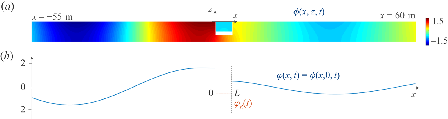
Meaning of the reduction of model. (a) The solution of the actual problem is computed numerically on the velocity potential  $\phi (x,z,t)$ solution of (2.1). (b) The solution of the reduced problem is computed for
 $\varphi (x,t)=\phi (x,0,t)$ for
 $x\notin (0,L)$ solution of (2.3) and
 $\varphi _{\scriptscriptstyle R}(t)=\phi (x,0,t)$ for
 $x\in (0,L)$ solution of (2.11) for an incident wave
 $\varphi _{\scriptscriptstyle {inc}}(x,t)$.

The effect of the resonator has been encapsulated in effective transmission conditions which constitute the main results of the present analysis. The first condition on the jump of the potential  $\left [\kern-1pt[ \varphi \right ]\kern-1pt]$ across the resonator (between
 $x=0$ and
 $x=L$) involves the mean value of the horizontal velocity. It is the condition obtained for a dock on its own. In this context,
 ${\mathcal {B}}$ is the blockage coefficient appearing in the problem of a perfect fluid flowing in a rigid duct containing a constriction having the form of the dock (Bartholomeusz Reference Bartholomeusz1958; Tuck Reference Tuck1975, see also Appendix A). The second condition links the jump of the horizontal velocity
 $\left [\kern-1pt[ \partial _{x} \varphi \right ]\kern-1pt]$ across the resonator to the second time derivative
 ${\ddot {\varphi }}_{\scriptscriptstyle {R}}(t)$ of
 $\varphi _{\scriptscriptstyle R}(t)$ which is the uniform velocity potential within the resonant cavity. Eventually, apart from the geometrical parameters, the model (2.3)–(2.11) involves a blockage coefficient
 ${\mathcal {B}}$ and a so-called effective length
 $e_{\scriptscriptstyle {eff}}$. The former has an explicit expression and the latter can be evaluated (see Appendix A); they read
 \begin{equation} \left\{\begin{array}{@{}ll} \displaystyle {\mathcal{B}}=\dfrac{L}{h^{-}}+2{\mathcal{B}}_\mu, & \mu=\dfrac{h^{-}}{H},\\ e_{\scriptscriptstyle{eff}}=e+\dfrac{\ell}{2}\left({\mathcal{B}}_\mu+{\mathcal{B}}_{\mu_0}\right), & \mu=\dfrac{\ell}{L}, \mu_0=\dfrac{\ell}{L_{\scriptscriptstyle{o}}}, \end{array}\right. \end{equation}
where  ${\mathcal {B}}_\mu$ is a function of
 $\mu$ only, defined by
 \begin{equation} {\mathcal{B}}_\mu=\frac{1}{\rm \pi} \frac{(\mu^2+1)}{\mu}\log\frac{1+\mu}{1-\mu}-\frac{2}{\rm \pi}\log\frac{4\mu}{1-\mu^2}. \end{equation}
2.3. D'Alembert formulation of the solutions
In the presence of a right-going incident wave  $\varphi _{\scriptscriptstyle {inc}}$, the reduced problem (2.3) can be solved explicitly using d'Alembert solutions (d'Alembert Reference D'Alembert1747). Specifically, we use that the solution can be written, denoting
 $c=\sqrt {gH}$, as
 \begin{equation} \varphi(x,t)= \left\{\begin{array}{@{}ll} \displaystyle \varphi_{\scriptscriptstyle{inc}}(t-x/c) + \varphi^{{-}}(t+x/c), & x\in (-\infty,0),\\ \varphi^{{\tiny +}}(t-(x-L)/c), & x\in (L,+\infty), \end{array}\right. \end{equation}
where  $\varphi ^{{\tiny +}}$ is the transmitted right-going wave and
 $\varphi ^{{-}}$ is the reflected left-going wave. From (2.6) we have
 $\left [\kern-1pt[ \varphi \right ]\kern-1pt] =\varphi ^{{\tiny +}}(t)-\varphi ^{{-}}(t)-\varphi _{\scriptscriptstyle {inc}}(t)$,
 $\overline { \partial _{x}{\varphi } }=-{1}/{2c}({\dot {\varphi }}^{{\tiny +}}(t)-{\dot {\varphi }}^{-}(t)+{\dot {\varphi }}_{\scriptscriptstyle {inc}}(t))$ and
 $\left [\kern-1pt[ \partial _{x} \varphi \right ]\kern-1pt] =-{1}/{c}({\dot {\varphi }}^{{\tiny +}}(t)+{\dot {\varphi }}^{-}(t)-{\dot {\varphi }}_{\scriptscriptstyle {inc}}(t))$. Reporting these expressions in the transmission conditions (2.3) we obtain that
 $\varphi _{\scriptscriptstyle {dock}}=(\varphi ^{{\tiny +}}-\varphi ^{{-}}-\varphi _{\scriptscriptstyle {inc}})/{2}$ and
 $\varphi _{\scriptscriptstyle {res}}=(\varphi ^{{\tiny +}}+\varphi ^{{-}}-\varphi _{\scriptscriptstyle {inc}})/{2}$ satisfy
 \begin{equation} \displaystyle {\dot{\varphi}}_{\scriptscriptstyle res}(t)={-}\frac{2}{\omega_0^2\tau}\, {\ddot{\varphi}}_{\scriptscriptstyle{R}}(t),\quad {\dot \varphi}_{\scriptscriptstyle{dock}}(t)+\frac{1}{\tau_{\scriptscriptstyle{dock}}}\varphi_{\scriptscriptstyle{dock}}(t)={-} {\dot{\varphi}}_{\scriptscriptstyle{inc}}(t), \end{equation}
where
 \begin{equation} \tau_{\scriptscriptstyle{dock}}=\frac{{\mathcal{B}}}{2}\sqrt{\frac{H}{g}}, \end{equation}
and where we have used that  ${c L_{\scriptscriptstyle {o}}}/{gH}={4}/{\omega _0^2\tau }$. Eventually, the waves emitted by the resonator are given by
 \begin{equation} \displaystyle \varphi^{{-}}(t)=\varphi_{\scriptscriptstyle{res}}(t)-\varphi_{\scriptscriptstyle{dock}}(t), \quad \displaystyle (\varphi^{{\tiny +}}(t)-\varphi_{\scriptscriptstyle{inc}}(t))=\varphi_{\scriptscriptstyle{res}}(t)+\varphi_{\scriptscriptstyle{dock}}(t), \end{equation}
from which we deduce that
 \begin{equation} \bar{\varphi}(t)=\varphi_{\scriptscriptstyle{inc}}(t)-\frac{2}{\omega_0^2\tau}{\dot{\varphi}}_{\scriptscriptstyle R}(t). \end{equation}
Hence, the harmonic oscillator equation in (2.3) that governs the potential  $\varphi _{\scriptscriptstyle R}$ inside the cavity takes the form
 \begin{equation} \left\{\begin{array}{@{}l} \displaystyle {\ddot{\varphi}}_{\scriptscriptstyle{R}}(t)+\dfrac{2}{\tau}\,{\dot{\varphi}}_{\scriptscriptstyle R}(t)+\omega_0^2\varphi_{\scriptscriptstyle R}(t)=\omega_0^2\,\varphi_{\scriptscriptstyle{inc}}(t),\\ \quad \text{where}\displaystyle \ \omega_0=\sqrt{\dfrac{g\ell}{e_{\scriptscriptstyle{eff}}L_{\scriptscriptstyle{o}}}}, \quad \tau=\dfrac{4e_{\scriptscriptstyle{eff}}}{\ell}\sqrt{\dfrac{H}{g}}, \end{array}\right. \end{equation}
which corresponds to the equation of a damped resonator, with  $\omega _0$ the resonance frequency and
 $\tau$ the characteristic time of the radiative damping due to the coupling of the resonator with the surrounding fluid. Eventually,
 $\varphi _{\scriptscriptstyle {inc}}(t-x/c)=\phi _{\scriptscriptstyle inc}(x,0,t)$ is the potential associated with the incident wave at the free surface.
The above general solution confirms the kind of contributions of the resonator and of the dock that were already visible from the transmission conditions in (2.3): the resonator acts as a monopole radiating  $\varphi _{\scriptscriptstyle {res}}(t)$ symmetrically toward
 $x<0$ and
 $x>L$; the dock on its own acts as a dipole radiating
 $\pm \varphi _{\scriptscriptstyle {dock}}(t)$ toward
 $x<0$ and
 $x>L$. Incidentally, we also obtain that
 $\bar {\varphi }(t)=\varphi _{\scriptscriptstyle {inc}}(t)+\varphi _{\scriptscriptstyle {res}}(t)$, which provides (2.10) using (2.7a,b). Eventually, with
 $\ell$ much smaller than the other dimensions of the problem, we have
 \begin{equation} \omega_0\tau=4\sqrt{\frac{e H}{L_{\scriptscriptstyle{o}}\ell}}\gg 1,\quad \omega_0\tau_{\scriptscriptstyle{dock}}=\frac{{\mathcal{B}}}{2}\sqrt{\frac{H\ell}{e L_{\scriptscriptstyle{o}}}}\ll 1. \end{equation}
The first relation tells us that, because of its thin neck, the resonator is weakly coupled to the surrounding water. In contrast, the response of the dock up to the resonance frequency (at least) is dictated by the incident wave, as  $\varphi _{\scriptscriptstyle {dock}}(t)\sim -\tau _{\scriptscriptstyle {dock}}{\dot {\varphi }}_{\scriptscriptstyle {inc}}(t)$.
3. Validation of the reduced problem in the harmonic regime
We start by analysing the reduced problem in the harmonic regime, in order to easily validate the reduced model by comparison to direct numerics. The numerics uses a classical multimodal method to compute the solution of the actual problem (2.1); the method is detailed in Appendix C.
The results presented in this section are obtained for the following geometry:  $H=6$ m,
 $L=5$ m,
 $L_{\scriptscriptstyle {o}}=4.8$ m,
 $e=1$ m,
 $\ell =0.1$ m,
 $h^{-}=2$ m (
 $h^{+}=3$ m) and we consider the frequency range
 $\omega \in (0,1) \ \textrm {rad}\ \textrm {s}^{-1}$. The resulting parameters are:
 $\tau _{\scriptscriptstyle {dock}}=1.35$ s,
 $\omega _0=0.40\ \textrm {rad}\ \textrm {s}^{-1}$ and
 $\tau =38.3$ s. (with
 ${\mathcal {B}}=3.45$ and
 $e_{\scriptscriptstyle {eff}}=1.22$ m).
3.1. Solution in the harmonic regime
In the harmonic regime at frequency  $\omega$, we denote
 $\varphi (x,t)=\textrm {Re}(\tilde \varphi (x,\omega ) \textrm {e}^{-\textrm {i}\omega t})$ and we consider an incident wave with unitary amplitude
 ${\tilde \varphi }_{\scriptscriptstyle {inc}}(x,\omega )=\textrm {e}^{\textrm {i}k x}$, where
 $k={\omega }/{\sqrt {gH}}$ is the wavenumber in
 $x\in (-\infty ,0)\cup (L,+\infty )$. The complex uniform potential
 ${\tilde {\varphi }}_{\scriptscriptstyle R}(\omega )$ in the cavity solution to (2.11) and the potentials
 ${\tilde \varphi }_{\scriptscriptstyle {dock}}(\omega )$ and
 ${\tilde {\varphi }}_{\scriptscriptstyle {res}}(\omega )$ solutions to (2.7a,b), read
 \begin{equation} \left\{\begin{array}{@{}l} \displaystyle {\tilde{\varphi}}_{\scriptscriptstyle R}(\omega)=\dfrac{\omega_0^2}{\left(\omega_0^2- \omega^2-\dfrac{2\textrm{i}\omega}{\tau}\right)}, \\ \displaystyle {\tilde \varphi}_{\scriptscriptstyle{dock}}(\omega)= \dfrac{\textrm{i}\omega\tau_{\scriptscriptstyle{dock}}}{\left(1-\textrm{i}\omega\tau_{\scriptscriptstyle{dock}}\right)}, \quad \displaystyle {\tilde{\varphi}}_{\scriptscriptstyle{res}}(\omega)= \dfrac{\dfrac{2\textrm{i}\omega}{\tau}}{\left(\omega_0^2- \omega^2-\dfrac{2\textrm{i}\omega}{\tau}\right)}. \end{array}\right. \end{equation}
Introducing the scattering coefficients  $(R,T)$ for the potential
 $\tilde {\varphi }$ in the form
 \begin{equation} \displaystyle \tilde \varphi(x<0,\omega)= \left(\textrm{e}^{\textrm{i}k x}+R(\omega)\textrm{e}^{-\textrm{i}k x}\right),\quad \displaystyle \tilde \varphi(x>L,\omega)= T(\omega) \textrm{e}^{\textrm{i}k (x-L)}, \end{equation}
and identifying with (2.6)–(2.9a,b) we obtain  $\tilde {\varphi }^-(\omega )=R(\omega )$ and
 $\tilde {\varphi }^+(\omega )=T(\omega )$, hence
 \begin{equation} \left\{\begin{array}{@{}l} \displaystyle R= \dfrac{1}{2}\dfrac{ \left(\omega_0^2- \omega^2+\dfrac{2\textrm{i}\omega}{\tau}\right)}{\left(\omega_0^2- \omega^2-\dfrac{2\textrm{i}\omega}{\tau}\right)} -\dfrac{1}{2}\dfrac{\left(1+\textrm{i}\omega\tau_{\scriptscriptstyle{dock}}\right)}{\left(1-\textrm{i}\omega\tau_{\scriptscriptstyle{dock}}\right)},\\ \displaystyle T= \dfrac{1}{2}\dfrac{ \left(\omega_0^2- \omega^2+\dfrac{2\textrm{i}\omega}{\tau}\right)}{\left(\omega_0^2- \omega^2-\dfrac{2\textrm{i}\omega}{\tau}\right)} +\dfrac{1}{2}\dfrac{\left(1+\textrm{i}\omega\tau_{\scriptscriptstyle{dock}}\right)}{\left(1-\textrm{i}\omega\tau_{\scriptscriptstyle{dock}}\right)}, \end{array}\right. \end{equation}
which satisfy  $|R|^2+|T|^2=1$. For the dock on its own,
 $\varphi _{\scriptscriptstyle R}=0$, resulting in
 \begin{equation} R_{\scriptscriptstyle dock}=\frac{1}{2}-\frac{1}{2}\frac{\left(1+\textrm{i}\omega\tau_{\scriptscriptstyle{dock}}\right)}{\left(1-\textrm{i}\omega\tau_{\scriptscriptstyle{dock}}\right)},\quad T_{\scriptscriptstyle{dock}}=1-R_{\scriptscriptstyle dock}. \end{equation}
Eventually, the amplitude within the cavity given by (3.1) reaches a maximum at the resonance with
 \begin{equation} {\tilde{\varphi}}_{\scriptscriptstyle R}(\omega_0)=\frac{\textrm{i}\omega_0\tau}{2}=2\textrm{i}\sqrt{\frac{e_{\scriptscriptstyle{eff}} H}{\ell L_{\scriptscriptstyle{o}}}}. \end{equation}
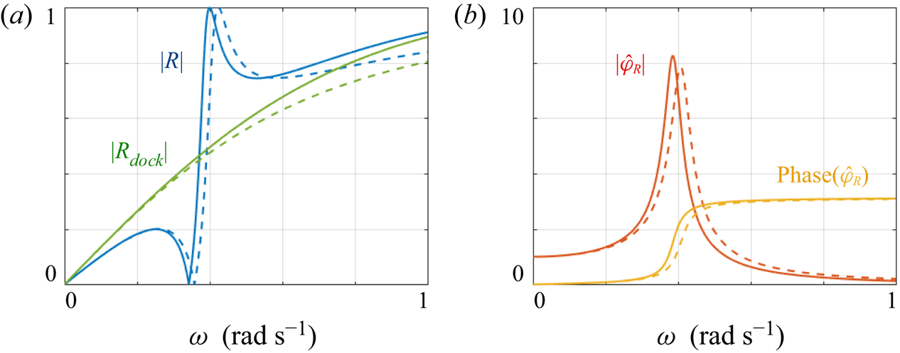
We have calculated numerically the solution of the actual problem (2.1) for  $\omega \in (0,1)\ \textrm {rad}\ \textrm {s}^{-1}$. We report in figure 3 the variations of
 $|R(\omega )|$ and
 ${\tilde {\varphi }}_{\scriptscriptstyle R}(\omega )$. In panel (a), we see that the resonance curve
 $|R(\omega )|$ has a highly asymmetric profile characteristic of a Fano resonance, with sharp variations producing perfect and zero reflection. We also report the underlying smooth curve corresponding to the background scattering of the dock on its own. In the context of water waves, similar variations have been reported in Parsons & Martin (Reference Parsons and Martin1994) due to Mie resonances occurring when a submerged obstacle rises to the free surface. Panel (b) shows the corresponding amplitude within the cavity with rapid variations in magnitude and phase (from 0 to
 ${\rm \pi}$). It is worth noticing that the resonance is deeply subwavelength with an incident wavelength
 $\lambda ={2{\rm \pi} \sqrt {gH}}/{\omega _0}$ 30 times larger than the dimensions,
 $L$ and
 $h^{+}$, of the resonator. The predictions of the reduced model,
 $R$ in (3.3),
 $R_{\scriptscriptstyle dock}$ in (3.4a,b) and
 ${\tilde {\varphi }}_{\scriptscriptstyle R}$ in (3.1), are in good agreement with the direct numerics with two distinct sources of discrepancy. On the one hand, in the vicinity of the resonance, we observe a systematic shift of around
 $0.02\ \textrm {rad}\ \textrm {s}^{-1}$ between the resonance curve calculated numerically and the theoretical one. Specifically, the model predicts a resonance frequency
 $\omega _0=0.41\ \textrm {rad}\ \textrm {s}^{-1}$ from (2.11) and a succession of a perfect reflection at
 $\omega _1$ and a perfect transmission at
 $\omega _2$ given, from (3.3), by
 \begin{equation} \omega_1=\sqrt{\omega_0^2- 2(\tau\tau_{\scriptscriptstyle{dock}})^{{-}1}},\quad \omega_2=\frac{\omega_0}{\sqrt{1-2 \tau_{\scriptscriptstyle{dock}}\tau^{{-}1}}}, \end{equation}
(in the present case,  $\omega _1=0.36\ \textrm {rad}\ \textrm {s}^{-1}$ and
 $\omega _2=0.42\ \textrm {rad}\ \textrm {s}^{-1}$) while the actual, numerical values are lower; this is attributable to the approximate added length which could be refined by conducting the analysis at higher order. On the other hand, the scattering strength of the dock on its own, measured here by
 $|R_{\scriptscriptstyle dock}|$, is underestimated by the model above
 $0.4\ \textrm {rad}\ \textrm {s}^{-1}$ (
 $kH\simeq 0.3$) as the assumption of the shallow water regime becomes less valid. As expected, the shift in the resonance frequency is recovered in the resonant curve
 ${\tilde {\varphi }}_{\scriptscriptstyle R}(\omega )$. However, the model reproduces correctly that the amplitude within the cavity is the same as outside for long waves (
 $\omega \to 0$) while it tends to zero for shorter waves. Indeed for these latter, the cavity behaves as a closed cavity.
Validation of the reduced model solution (dashed lines) by comparison to direct numerical calculations (plain lines). (a) Reflection coefficient  $|R(\omega )|$ against
 $\omega \in (0,1)\ \textrm {rad}\ \textrm {s}^{-1}$; for comparison,
 $|R_{\scriptscriptstyle dock}|$ for a dock on its own (
 $\ell =0$) is reported. In the reduced model, we use (3.3)–(3.4a,b). (b) Velocity potential
 ${\tilde {\varphi }}_{\scriptscriptstyle R}(\omega )$ (magnitude and phase) within the resonator. In the reduced model we use (3.1).

The two-dimensional fields  $\tilde {\phi }(x,z,\omega )$ computed numerically at the frequencies
 $\omega _1$ and
 $\omega _2$ are shown in figure 4. In both cases, the large amplitude within the cavity is constant although a zoom reveals strong contributions of the evanescent field excited at the ends of the neck (not shown) that are taken into account by added lengths. With
 $\omega _1<\omega _0<\omega _2$, and according to the phase variations in figure 3, the perfect transmission corresponds to an oscillation within the cavity in phase with the incident wave at
 $x=0$. Conversely, the perfect reflection corresponds to an oscillation within the cavity oscillating in phase quadrature with the incident wave at
 $x=0$. This is also visible from (3.1), along with (2.12a,b) and (3.6a,b). Accounting for the small shift in the reflection curves between the numerics and the model, we also report the profiles of the potential at the free surface outside and inside the cavity. Again, the agreement is good, in particular the constant shape of
 ${\tilde {\varphi }}_{\scriptscriptstyle R}$ in the cavity is confirmed.
Two-dimensional fields  $\tilde \phi (x,z,\omega )$ and corresponding profiles
 $\tilde \varphi (x,\omega )$ at the free surface at
 $\omega =\omega _1$ (perfect transmission) and
 $\omega _2$ (perfect reflection). The profiles show
 $\tilde \varphi (x,\omega )$ outside the resonator (blue lines) and
 ${\tilde {\varphi }}_{\scriptscriptstyle R}(\omega )$ inside the cavity (red lines). The plain lines show the numerical results and the dashed lines the results of the model (3.2a,b)–(3.3).

3.2. From the shallow to the deep water-wave regime
Our analysis has been conducted in the shallow water regime which allows us to obtain a one-dimensional reduced model. However, most of the asymptotic analysis is done in the vicinity of the resonator independently of the water depth (see Appendix B). Thus, it makes sense to inspect whether or not the model remains predictive when we move from the shallow water regime to the finite depth regime. We have computed numerically the potential  ${\tilde {\varphi }}_{\scriptscriptstyle R}(\omega )$ for various
 $H\in (4,100)$ m. The result is shown in the inset of figure 5(a). We observe that the frequency
 $\omega _0$ realizing the maximum is independent of
 $H$ and it agrees with (2.3). This confirms that the resonance frequency is characteristic of the resonator on its own. Next, the resonant amplitude
 $|{\tilde {\varphi }}_{\scriptscriptstyle R}(\omega _0)|$ increases with
 $H$ for small
 $H$ in agreement with (3.5), afterwards, it saturates (above
 $H\simeq 40 \ \textrm {m}$ in the main plot in (a)). In the shallow water regime, the increase of the resonant amplitude with
 $H$ tells us that the presence of the sea bottom below the cavity weakens the resonance; a similar confinement effect has been reported for acoustic HRs (Maurel et al. Reference Maurel, Pham and Marigo2019). However, as the water depth increases, this effect vanishes and the amplitude tends to a value corresponding to the resonance in the deep water regime (hence, independent of
 $H$).
From shallow (SW) to deep water (DW). (a) Variations of  ${\tilde {\varphi }}_{\scriptscriptstyle R}(\omega _0)$ against
 $H$, calculated numerically (plain line) and from (3.5) (dashed lines). The inset shows
 ${\tilde {\varphi }}_{\scriptscriptstyle R}$ in colour scale against
 $\omega$ and
 $H$ calculated numerically; the dashed white line shows
 $\omega =\omega _0$ from (2.3). (b,c) Show
 $|R(\omega )|$ and
 ${\tilde {\varphi }}_{\scriptscriptstyle R}(\omega )$ for
 $H=50$ m, same representation as in figure 3. The inset in panel (c) shows
 $\lambda (\omega )$ moving from the SW to the DW regime.

Panels (b,c) show  $|R(\omega )|$ and
 ${\tilde {\varphi }}_{\scriptscriptstyle R}(\omega )$ for the intermediate water depth
 $H=50\ \textrm {m}$. The shape of the resonance curve differs significantly from that reported in the shallow water regime in figure 3. The main reason is that the scattering strength of the dock on its own is weak around the resonance. As in figure 3, we report for comparison the predictions for
 ${\tilde {\varphi }}_{\scriptscriptstyle R}$ from (3.1),
 $R$ from (3.3) and
 $R_{\scriptscriptstyle dock}$ from (3.4a,b). The most noticeable error in the reduced model is already visible on
 $R_{\scriptscriptstyle dock}$ which is underestimated for
 $\omega > 0.2\ \textrm {rad}\ \textrm {s}^{-1}$. The same occurs for
 $R$ as
 $R$ tends to
 $R_{\scriptscriptstyle dock}$ outside the resonance. The shallow water approximation used in the model overestimates the wavelength, hence it erroneously predicts that the wave can pass easily through the dock. In the reported case, the reflection is significant, up to 4 times the value predicted by the shallow water approximation (at
 $\omega =1\ \textrm {rad}\ \textrm {s}^{-1}$). In contrast, the overall variations of the amplitude
 ${\tilde {\varphi }}_{\scriptscriptstyle R}$ in the cavity are well reproduced by the reduced model (we know from (a) that the maximum is overestimated). Below the resonance, the cavity behaves as an open cavity,
 $|{\tilde {\varphi }}_{\scriptscriptstyle R}|=1$ is dictated by the incident wave of amplitude unity. Above the resonance it behaves as a close cavity with
 $|{\tilde {\varphi }}_{\scriptscriptstyle R}|=0$. These trends are robust whatever the water depth. Additional refinements would be necessary to restore the effect of wave dispersion which affects the amplitude within the resonator and the effect of the dock on its own.
4. Dynamics of the resonator in the transient regime
4.1. Solutions for an incident wave packet in the transient signal
We now move on to the dynamics of the resonator in the transient regime. As previously said, the solution of the reduced problem is still explicit. Given an incident wave packet  $\varphi _{\scriptscriptstyle {inc}}(x,t)$, the solution
 $\varphi _{\scriptscriptstyle R}(t)$ is known as it simply requires us to solve the equation of a damped oscillator forced with
 $\varphi _{\scriptscriptstyle {inc}}(0,t)$ in (2.11). We consider
 $\varphi _{\scriptscriptstyle R}(0,t=0)={\dot {\varphi }}_{\scriptscriptstyle R}(0,t=0)=0$ as initial conditions corresponding to a source switched on at
 $t=0$. Next, we have from (2.7a,b) that
 \begin{equation} \displaystyle \varphi_{\scriptscriptstyle{res}}(t)={-}\frac{2}{\omega_0^2\tau}\,{\dot{\varphi}}_{\scriptscriptstyle R}(t), \quad \varphi_{\scriptscriptstyle{dock}}(t)={-} \int_0^t{\dot{\varphi}}_{\scriptscriptstyle{inc}}(t')\textrm{e}^{-(t-t')/\tau_{\scriptscriptstyle{dock}}}\,\text{d}t', \end{equation}
as  $\varphi _{\scriptscriptstyle {dock}}(t=0)=0$. Eventually, the above solutions are used in (2.9a,b) to get the whole solution (2.6), with
 $\varphi ^\pm (t)$ in (2.9a,b) the wave packets radiated by the resonator.
To begin with, we consider an incident short pulse of the form
 \begin{equation} \varphi_{\scriptscriptstyle{inc}}(0,t)= \textrm{e}^{-\tau_{\scriptscriptstyle{f}}^{{-}2} (t-t_i)^2}, \end{equation}
with  $\tau _{\scriptscriptstyle {f}}=3$ s (and
 $t_i=15$ s) whose significant spectral content is within the interval
 $\omega \in (0,2)\ \textrm {rad}\ \textrm {s}^{-1}$. The pulse is much shorter than the damping time
 $\tau =38$ s, which provides a rough idea of the impulse response of the system. Figure 6(a) shows the incident pulse
 $\varphi _{\scriptscriptstyle {inc}}(0,t)$ and the resulting uniform potential within the cavity whose dynamics is that of an underdamped harmonic oscillator driven by
 $\varphi _{\scriptscriptstyle {inc}}(0,t)$. Panel (b) shows the corresponding variations of the radiated signals
 $\varphi _{\scriptscriptstyle {res}}(t)$ and
 $\varphi _{\scriptscriptstyle {dock}}(t)$, from (4.1a,b). Expectedly, we observe that
 $\varphi _{\scriptscriptstyle {dock}}(t)\simeq -\tau _{\scriptscriptstyle {dock}} {\dot {\varphi }}_{\scriptscriptstyle {inc}}(t)$ and thus it is as short as the initial pulse. In contrast,
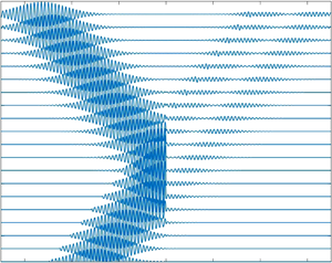
 $\varphi _{\scriptscriptstyle {res}}(t)$ has a long regime of free oscillations, being weakly radiatively damped. To complete this representation, we report in figure 7 snapshots of the potential
 $\varphi (x,t)$ at the free surface and a profile for
 $t=120$ s. It is visible that the transmitted and reflected pulses resulting from the direct interaction with the incident pulse are followed by long right- and left-going wave trains radiated by the resonator (the segment
 $(0,L)$ is almost reduced to the origin in this representation).
(a) Time variation of the amplitude  $\varphi _{\scriptscriptstyle R}(t)$ within the resonator for an incident short pulse
 $\varphi _{\scriptscriptstyle {inc}}(0,t)$. (b) Resulting
 $\varphi _{\scriptscriptstyle {res}}(t)$ and
 $\varphi _{\scriptscriptstyle {dock}}(t)$ from (4.1a,b).

(a) Snapshots of the potential  $\varphi (x,t)$ at the free surface,
 $x\notin (0,L)$, with
 $c=\sqrt {gH}\simeq 5.3\ \textrm {m}\ \textrm {s}^{-1}$. (b) Profile of
 $\varphi (x,120\ \text {s})$; the oscillator emits
 $\varphi ^+(0,t)$ and
 $\varphi ^-(0,t)$.

We now inspect the ability of the HR to realize perfect transmission and perfect reflection in the transient regime. To do so, we use an incident wave packet able to excite more specifically a given frequency, namely we use
 \begin{equation} \varphi_{\scriptscriptstyle{inc}}(0,t)=a \exp({-\tau_{\scriptscriptstyle{f}}^{{-}2} (t-t_i)^2})\sin(\omega_{\scriptscriptstyle f}(t-t_i)), \end{equation}
with  $\omega _{\scriptscriptstyle f}$ the forcing frequency,
 $\tau _{\scriptscriptstyle {f}}$ the width of the Gaussian envelope and
 $a$ such that
 $\textrm {Max}(\varphi _{\scriptscriptstyle {inc}}(0,t))=1$. We choose
 $\omega _{\scriptscriptstyle f}=\omega _1$ and
 $\omega _{\scriptscriptstyle f}=\omega _2$, the frequencies realizing perfect transmission and perfect reflection in the harmonic regime, from (3.6a,b); for comparison, we also consider
 $\omega _{\scriptscriptstyle f}=\omega _0$. For these 3 frequencies we set the incident pulse duration to
 $\tau _{\scriptscriptstyle {f}}=140$ s (approximately 40 oscillation periods). Results are shown in figure 8, where we report
 $\varphi _{\scriptscriptstyle {inc}}(0,t)$ and the resulting
 $\varphi _{\scriptscriptstyle R}(t)$, and figure 9, where we report the snapshots of
 $\varphi (x,t)$ and a zoom on
 $\varphi _{\scriptscriptstyle R}(x,600$ s). With a time scale variation of the incident pulse greater than the free oscillation period, the regime of oscillations driven by the forcing incident signal dominates and the free oscillation regime is almost negligible. Hence, both
 $\varphi _{\scriptscriptstyle {res}}$ and
 $\varphi _{\scriptscriptstyle {dock}}$ have almost the same duration as the incident wave packet and this is required in order to produce perfect transmission and perfect reflection. Indeed, perfect transmission results from destructive interference between the two radiated waves
 $\varphi _{\scriptscriptstyle {res}}$ and
 $\varphi _{\scriptscriptstyle {dock}}$ (hence
 $\varphi ^-=0$). Perfect reflection is in some sense more demanding as it results from destructive interference between
 $\varphi _{\scriptscriptstyle {res}}$,
 $\varphi _{\scriptscriptstyle {dock}}$ and
 $\varphi _{\scriptscriptstyle {inc}}$ as we want
 $\varphi ^+=0$. As these conditions cannot be perfectly met, imperfect complete transmission and reflection are observed. Nevertheless, the enhancement in reflection for
 $\omega _{\scriptscriptstyle f}=\omega _1$ and in transmission for
 $\omega _{\scriptscriptstyle f}=\omega _2$ is visible when compared with the reference case at
 $\omega =\omega _0$.
Incident pulse  $\varphi _{\scriptscriptstyle {inc}}(0,t)$ from (4.3) (blue lines) and corresponding
 $\varphi _{\scriptscriptstyle R}(t)$ (red lines) (a)
 $\omega _{\scriptscriptstyle f}=\omega _1$ producing perfect transmission in the harmonic regime, (b)
 $\omega _{\scriptscriptstyle f}=\omega _0$ the resonance frequency and (c)
 $\omega _2$ producing a perfect reflection in the harmonic regime (see (3.6a,b)).


5. Concluding remarks
We have studied an analogue of the acoustic HR in the context of water waves. As for its acoustic analogue, the lowest resonance is deeply subwavelength thanks to a thin neck connecting the cavity to the surrounding water. Obviously, this subwavelength property is of importance to the design of objects with the objective to control water waves of very long wavelength. The small dimensions of the whole device compared with the wavelength makes possible the use of asymptotic analysis and the derivation of a one-dimensional reduced model in the shallow water regime. The model has been validated in the harmonic regime by comparison to direct numerics; afterwards, solutions in the transient regime have been sought.
The present analysis has been done in the idealized case of linear waves in an inviscid fluid; the resulting one-dimensional model corresponds to the dominant non-trivial asymptotic order. Within these assumptions, pursuing the calculations to the second order would allow us to capture more subtle effects such as the position of the neck connected to the cavity (here located on the bottom horizontal wall of the cavity but which can be positioned on a vertical wall, the two vertical walls playing a non-symmetric role for the incoming wave). Other extensions consist in including the effect of the losses due to the viscosity that we expect to be significant in the neck or due to nonlinearities within the cavity as the velocity reaches large values. Although this can be done by adding heuristically a damping term in the equation of the resonator (2.11), as in Monsalve et al. (Reference Monsalve, Maurel, Petitjeans and Pagneux2019), these ingredients can by explicitly accounted for in the analysis, see Caflisch et al. (Reference Caflisch, Miksis, Papanicolaou and Ting1985) for viscous effects and Pham et al. (Reference Pham, Mercier, Fuster, Marigo and Maurel2020) for nonlinear effects. We have in mind the perfect absorption obtained with acoustic HRs (Romero-García et al. Reference Romero-García, Jimenez, Theocharis, Achilleos, Merkel, Richoux, Tournat, Groby and Pagneux2020) and for water waves in reflection (Monsalve et al. Reference Monsalve, Maurel, Petitjeans and Pagneux2019). Another interesting extension would be to use a series of different resonators to obtain broadband behaviours (Jiménez et al. Reference Jiménez, Romero-García, Pagneux and Groby2017; Bennetts et al. Reference Bennetts, Peter and Craster2018).
Funding
V.P., P.P. and A.M. thank the supports of the start-up Bluerium. K.P. thanks the supports of the Agence de l'Innovation de Défense (AID) from the Direction Générale de l'Armement (DGA), under grant 2019 65 0070.
Declaration of interests
The authors report no conflict of interest.
Author contributions
Conceptualization, L.-P.E.; theoretical model and numerical method, A.M., K.P.; writing of the manuscript, A.M. and K.P.; correction of the manuscript, L.-P.E., A.M., K.P., P.P., V.P. All authors have read and agreed to the published version of the manuscript.
Appendix A. Remark on the blockage coefficients and added lengths
Simple expressions for the effective length  $e_{\scriptscriptstyle {eff}}$ and blockage coefficient
 ${\mathcal {B}}$ are given here. What we need is the result of Tuck (Reference Tuck1977), which provides the blockage coefficient of a step reducing the water depth from
 $H^+$ to
 $H^-< H^+$ (figure 10a). With
 $\mu ={H^-}/{H^+}$ it reads
 \begin{equation} {\mathcal{B}}_\mu=\frac{1}{\rm \pi} \frac{(\mu^2+1)}{\mu}\log\frac{1+\mu}{1-\mu}-\frac{2}{\rm \pi}\log\frac{4\mu}{1-\mu^2}. \end{equation}
This coefficient appears in the jump of the potential which reads as  $(\varphi ^+-\varphi ^-)={\mathcal {B}}_\mu D$ at the section discontinuity while the flow rate is continuous
 $D=H^+\partial _{x}\varphi ^+=H^-\partial _{x}\varphi ^-$. Owing to this result, it is possible to extrapolate the blockage coefficient
 ${\mathcal {B}}$ in problem (b) and the effective length
 $e_{\scriptscriptstyle {eff}}$ in problem (c) of figure 10.
(a) The problem of a perfect fluid flowing in a rigid duct with a sudden change in height ( $H^+\to H^-$) involving the blockage coefficient
 ${\mathcal {B}}_\mu$,
 $\mu ={H^-}/{H^+}$. (b) The problem of a perfect fluid flowing in a rigid duct with two sudden changes in height
 $H\to h^{-}\to H$ involves a blockage coefficient
 ${\mathcal {B}}$. (c) The problem of a perfect fluid flowing through a duct with three sudden changes in height (
 $L\to \ell \to L_{\scriptscriptstyle {o}}$) involves a blockage coefficient
 ${\mathcal {B}}_{{\scriptscriptstyle n}}$.

We begin with problem (b). As the effect of the evanescent fields at  $x=0$ and
 $x=L$ is encapsulated in
 ${\mathcal {B}}_\mu$, the solution can be written
 \begin{equation} \varphi(x<0)=\frac{x}{H},\quad \varphi(0< x< L)=\frac{x}{h^{-}}+\alpha,\quad \varphi(x>L)=\frac{(x-L)}{H}+{\mathcal{B}}, \end{equation}
which already satisfies the continuity of the flow rate  $D=1$. Applying further
 $\varphi (0^+)-\varphi (0^-)={\mathcal {B}}_\mu$ and
 $\varphi (L^+)-\varphi (L^-)={\mathcal {B}}_\mu$, we obtain
 $\alpha ={\mathcal {B}}_\mu$ and
 \begin{equation} {\mathcal{B}}=\frac{L}{h^{-}}+2{\mathcal{B}}_\mu,\quad \mu=\frac{h^{-}}{H}. \end{equation}
We now move on to problem (c), which is the problem involving the added length in the neck of the resonator (we used mirror symmetry). We do the same as previously with
 \begin{equation} \varphi(x<0)=\frac{2x}{L},\quad \varphi(0< x< e)=\frac{2x}{\ell}+\beta,\quad \varphi(x>e)=\frac{(x-e)}{L_{\scriptscriptstyle{o}}}+{\mathcal{B}}_{\scriptscriptstyle N}, \end{equation}
which satisfies  $D=1$. Applying further
 $\varphi (0^+)-\varphi (0^-)={\mathcal {B}}_\mu$ (with
 $\mu ={\ell }/{L}$) and
 $\varphi (e^+)-\varphi (e^-)={\mathcal {B}}_{\mu _0}$ (with
 $\mu _0={\ell }/{L_{\scriptscriptstyle {o}}}$), we obtain
 $\beta ={\mathcal {B}}_\mu$ and
 \begin{equation} {\mathcal{B}}_{\scriptscriptstyle N}=\frac{2e}{\ell}+{\mathcal{B}}_\mu+{\mathcal{B}}_{\mu_0},\quad \mu=\frac{\ell}{L},\quad \mu_0=\frac{\ell}{L_{\scriptscriptstyle{o}}}. \end{equation}
Next, the effective length  $e_{\scriptscriptstyle {eff}}$ is by definition the length such that the constant velocity in
 $(0,e)$ satisfies
 \begin{equation} v|_{N}=\frac{2}{\ell}=\frac{\varphi(e^+)-\varphi(0^-)}{e_{\scriptscriptstyle{eff}}}, \end{equation}
which implies
 \begin{equation} e_{\scriptscriptstyle{eff}}=\frac{\ell}{2}{\mathcal{B}}_\text{N}=e+\frac{\ell}{2}\left({\mathcal{B}}_\mu+{\mathcal{B}}_{\mu_0}\right). \end{equation}
The above result is consistent with the analysis of Mercier, Marigo & Maurel (Reference Mercier, Marigo and Maurel2017) (owing to  ${\mathcal {B}}_\mu \simeq -({2}/{{\rm \pi} })\log (\sin (({{\rm \pi} }/{2})\mu ))$). It is worth noting that the blockage coefficient in (A3a,b) appears explicitly in the asymptotic analysis, see (B26a–b). In contrast, the effective length (A7) is introduced heuristically as the analysis provides only the actual length of the neck, see (B46a,b) (an effective length would appear at the following asymptotic order).
Appendix B. Asymptotic analysis
In this section, we shall derive the reduced model (2.3) thanks to asymptotic analysis. This will be done by defining a small parameter  $\varepsilon$ and by choosing scalings for all the dimensions of the problem.
B.1. The choice of the scalings
The heuristic calculation leading to (1.2) is used to set the scalings. This calculation is done assuming that the cavity has dimensions much smaller than the incident wavelength, and that the cavity is disconnected from the surrounding fluid, resulting in a zero velocity and a constant potential at the dominant order. What we want to obtain with the scalings is that the non-dimensional frequency remains of the order of the resonance frequency asymptotically. In the most general case, defining  $\varepsilon =kD$ with
 $D$, a measure of the cavity extent, this means
 \begin{equation} \frac{\omega_0}{c}D=\frac{D}{c}\sqrt{ \frac{g\ell}{e L_{\scriptscriptstyle{o}}}}=O(\varepsilon), \end{equation}
with  $c$ the velocity of the water waves. The above relation holds for a wave in shallow to deep water. In our study, we focus on the shallow water regime where
 $c=\sqrt {gH}$ and we assume that
 $H$ and the dimensions of the cavity
 $(L,L_{\scriptscriptstyle {o}},h^{+})$ tend to 0 as fast as
 $H$ when
 $\varepsilon$ vanishes. Defining
 $\varepsilon =kH$, we obtain that the geometry of the neck must satisfy
 \begin{equation} \sqrt{\frac{\ell}{e}}=O(\varepsilon). \end{equation}
This means that  $\ell$ has to decrease faster than
 $e$ when
 $\varepsilon \to 0$ and the simplest scaling to guarantee this is given by
 $ke=O(\varepsilon )$ and
 $k\ell =O(\varepsilon ^3)$. We thus expect that the fields have variations associated with three scales, the macroscopic wavelength scale, the mesoscopic scales being the typical scale of the dock and the microscopic scale associated with the neck opening.
B.2. Non-dimensional formulation
We use a non-dimensional problem by setting  $t\to \omega t$,
 ${\boldsymbol {x}}\to k{\boldsymbol {x}}$,
 $\boldsymbol {u}\to \boldsymbol {u}/U_0$ and
 $\phi \to k\phi /U_0$, with
 $k={\omega }/{\sqrt {g H}}$ and
 $U_0$ a characteristic velocity. The result consists in finding the potential
 $\phi$ and the velocity field
 $\boldsymbol {u}=(u,v)$ such that (2.1)–(2.2a,b) read
 \begin{equation} \begin{cases} {\rm{div}}\, \boldsymbol{u}=\textbf{0},\quad \boldsymbol{u}={\boldsymbol{\nabla}}\phi,\\ v|_{{z}=0}={-}\varepsilon\displaystyle\partial_{t t} \phi,\quad \boldsymbol{u}\cdot {\boldsymbol{n}}|_\varGamma=0, \end{cases} \end{equation}
where  $\varepsilon =\omega \sqrt {{H}/{g}}\ll 1$ is a small parameter.
B.3. The different regions and their matchings
B.3.1. The regions far from and near the resonator
(i) The macroscopic region far from the resonator
The macroscopic region corresponds to the region far from the resonator where the evanescent field is negligible and the fields vary at the scale of the incident wavelength. There, we rescale the vertical coordinate due to the shallowness hypothesis introducing  $\displaystyle z_{\scriptscriptstyle {m}}={z}/\varepsilon$ and we expand the potential and the velocity as
 \begin{align} \phi=\phi^0(x,z_{\scriptscriptstyle{m}},t)+\varepsilon\phi^1(x,z_{\scriptscriptstyle{m}},t)+\cdots,\quad \boldsymbol{u}=\boldsymbol{u}^0(x,z_{\scriptscriptstyle{m}},t)+\varepsilon\boldsymbol{u}^1(x,z_{\scriptscriptstyle{m}},t)+\cdots,\end{align}
with  $\boldsymbol {u}^i=(u^i,v^i)$. In this region, the differential operators read
 \begin{equation} {\boldsymbol{\nabla}} f=\partial_{x} f {\boldsymbol{e}}_x+{\varepsilon}^{{-}1}\partial_{z_{\scriptscriptstyle{m}}}{\,f}{\boldsymbol{e}}_z,\quad {\rm{div}}\, {\boldsymbol{f}}=\partial_{x} {f_x}+\varepsilon^{{-}1}\partial_{z_{\scriptscriptstyle{m}}}{\,f_z}. \end{equation}
(ii) The mesoscopic regions, near the resonator but far from its neck
The resonator has a characteristic size, apart of the neck, satisfying  $kh^{+}\sim \varepsilon$ and
 $kL\sim \varepsilon$. Accordingly, we introduce the mesoscopic space variable
 $\displaystyle (x_{\scriptscriptstyle {m}},z_{\scriptscriptstyle {m}})=(x /\varepsilon ,{z}/\varepsilon )$. Near the resonator and far from the neck, we distinguish two different mesoscopic regions. One is an unbounded domain
 $\hat {\varOmega }_{\scriptscriptstyle {{m}}}$ outside the resonator and the other is the bounded domain
 $\check {\varOmega }_{\scriptscriptstyle {{m}}}$ of the resonator cavity (figure 11). Accordingly we consider the two asymptotic expansions
 \begin{align} \begin{cases} \phi=\hat{\phi}_{\scriptscriptstyle{{m}}}^0(x_{\scriptscriptstyle{m}},z_{\scriptscriptstyle{m}},t)+\varepsilon\hat{\phi}_{\scriptscriptstyle{{m}}}^1(x_{\scriptscriptstyle{m}},z_{\scriptscriptstyle{m}},t)+\cdots, & \boldsymbol{u}=\hat{\boldsymbol u}_{\scriptscriptstyle{{m}}}^0(x_{\scriptscriptstyle{m}},z_{\scriptscriptstyle{m}},t)+\varepsilon\hat{\boldsymbol u}_{\scriptscriptstyle{{m}}}^1(x_{\scriptscriptstyle{m}},z_{\scriptscriptstyle{m}},t)+\cdots,\\ \phi=\check{\phi}_{\scriptscriptstyle{{m}}}^0(x_{\scriptscriptstyle{m}},z_{\scriptscriptstyle{m}},t)+\varepsilon\check{\phi}_{\scriptscriptstyle{{m}}}^1(x_{\scriptscriptstyle{m}},z_{\scriptscriptstyle{m}},t)+\cdots, & \boldsymbol{u}=\check{\boldsymbol{u}}_{\scriptscriptstyle{{m}}}^0(x_{\scriptscriptstyle{m}},z_{\scriptscriptstyle{m}},t)+\varepsilon\check{\boldsymbol{u}}_{\scriptscriptstyle{{m}}}^1(x_{\scriptscriptstyle{m}},z_{\scriptscriptstyle{m}},t)+\cdots, \end{cases} \end{align}
with  $\hat {\boldsymbol u}_{\scriptscriptstyle {{m}}}^i=(\hat {u}_{\scriptscriptstyle {{m}}}^i,\hat {v}_{\scriptscriptstyle {{m}}}^i)$ and
 $\check {\boldsymbol {u}}_{\scriptscriptstyle {{m}}}^i=(\check {u}_{\scriptscriptstyle {{m}}}^i,\check {v}_{\scriptscriptstyle {{m}}}^i)$, and the connection between them will be obtained through an asymptotic analysis in the vicinity of the neck. In these regions, the differential operators read
 \begin{equation} {\boldsymbol{\nabla}} f=\varepsilon^{{-}1}{\boldsymbol{\nabla}}_{\scriptscriptstyle{m}}\, f,\quad {\rm{div}}\, {\boldsymbol{f}}=\varepsilon^{{-}1}{\rm{div}}_{\scriptscriptstyle{m}}\, {\boldsymbol{f}}. \end{equation}
The two mesoscopic regions:  $\hat {\varOmega }_{\scriptscriptstyle {{m}}}$ being the unbounded region outside the cavity and
 $\check {\varOmega }_{\scriptscriptstyle {{m}}}$ the bounded region within the cavity. The ends of the neck are reduced to the points
 $\hat {N}$ and
 $\check {N}$ at this scale. The lengths are rescaled with
 $H$, hence
 $d_{\scriptscriptstyle {{m}}}={d}/{H}=O(1)$, for
 $d=L,L_{\scriptscriptstyle {o}},h^{+},h^{-},e$.

(iii) Along the neck and at its ends
The neck is thin and long and this is accounted for by setting  $ke \sim \varepsilon$ and
 $k\ell \sim \varepsilon ^3$. By zooming on the neck, we have thus to distinguish three different regions: inside the neck i.e. far from its ends, near the top end and near the bottom end. We introduce the microscopic space variables
 $\displaystyle (x_{\scriptscriptstyle \mu },z_{\scriptscriptstyle \mu })=(x /\varepsilon ^3,{z}/\varepsilon ^3)$. Inside the neck, we define the expansions
 \begin{align} \phi=\phi_{\scriptscriptstyle{\mu}}^0(x_{\scriptscriptstyle\mu},z_{\scriptscriptstyle{m}},t)+\varepsilon\phi_{\scriptscriptstyle{\mu}}^1(x_{\scriptscriptstyle\mu},z_{\scriptscriptstyle{m}},t)+\cdots,\quad \boldsymbol{u}=\varepsilon^{{-}1}\boldsymbol{u}_{\scriptscriptstyle{\mu}}^{{-}1}(x_{\scriptscriptstyle\mu},z_{\scriptscriptstyle{m}},t)+\boldsymbol{u}_{\scriptscriptstyle{\mu}}^0(x_{\scriptscriptstyle\mu},z_{\scriptscriptstyle{m}},t)+\cdots,\end{align}
with  $\boldsymbol {u}_{\scriptscriptstyle {\mu }}^i=(u_{\scriptscriptstyle {\mu }}^i,v_{\scriptscriptstyle {\mu }}^i)$ and
 \begin{equation} {\boldsymbol{\nabla}} f={\varepsilon}^{{-}3} \partial_{x_{\scriptscriptstyle\mu}}{f}{\boldsymbol{e}}_x+{\varepsilon}^{{-}1}\partial_{z_{\scriptscriptstyle{m}}}{\,f}{\boldsymbol{e}}_z,\quad {\rm{div}}\, {\boldsymbol{f}}={\varepsilon}^{{-}3} \partial_{x_{\scriptscriptstyle\mu}}{f_x}+\varepsilon^{{-}1}\partial_{z_{\scriptscriptstyle{m}}}{\,f_z}. \end{equation}
Near the top end and bottom end of the neck, we use
 \begin{align} \begin{cases} \phi=\hat{\phi}_{\scriptscriptstyle{\mu}}^0(x_{\scriptscriptstyle\mu},z_{\scriptscriptstyle\mu},t)+\varepsilon\hat{\phi}_{\scriptscriptstyle{\mu}}^1(x_{\scriptscriptstyle\mu},z_{\scriptscriptstyle\mu},t)+\cdots, & \boldsymbol{u}=\varepsilon^{{-}1}\hat{\boldsymbol u}_{\scriptscriptstyle{\mu}}^{{-}1}(x_{\scriptscriptstyle\mu},z_{\scriptscriptstyle\mu},t)+\hat{\boldsymbol u}_{\scriptscriptstyle{\mu}}^0(x_{\scriptscriptstyle\mu},z_{\scriptscriptstyle\mu},t)+\cdots,\\ \phi=\check{\phi}_{\scriptscriptstyle{\mu}}^0(x_{\scriptscriptstyle\mu},z_{\scriptscriptstyle\mu},t)+\varepsilon\check{\phi}_{\scriptscriptstyle{\mu}}^1(x_{\scriptscriptstyle\mu},z_{\scriptscriptstyle\mu},t)+\cdots, & \boldsymbol{u}=\varepsilon^{{-}1}\check{\boldsymbol u}_{\scriptscriptstyle{\mu}}^{{-}1}(x_{\scriptscriptstyle\mu},z_{\scriptscriptstyle\mu},t)+\check{\boldsymbol u}_{\scriptscriptstyle{\mu}}^0(x_{\scriptscriptstyle\mu},z_{\scriptscriptstyle\mu},t)+\cdots,\end{cases} \end{align}
with  $\hat {\boldsymbol u}_{\scriptscriptstyle {\mu }}^i=(\hat {u}_{\hspace {-0.02cm}\scriptscriptstyle {\mu }}^i,\hat {v}_{\scriptscriptstyle {\mu }}^i)$ and
 $\check {\boldsymbol u}_{\scriptscriptstyle {\mu }}^i=(\check {u}_{\scriptscriptstyle {\mu }}^i,\check {v}_{\scriptscriptstyle {\mu }}^i)$ (figure 12), and
 \begin{equation} {\boldsymbol{\nabla}} f={\varepsilon}^{{-}3} {\boldsymbol{\nabla}}_{\scriptscriptstyle\mu}{f},\quad {\rm{div}}\, {\boldsymbol{f}}={\varepsilon}^{{-}3} {\rm{div}}_{\scriptscriptstyle\mu}\, \boldsymbol{f}. \end{equation}
Note that we start the expansions for the velocity at the order  $\varepsilon ^{-1}$ to match the resonant behaviour of the cavity (other choices would lead to inconsistencies).
The three microscopic regions: (a) in the vicinity of the top of the neck, (b) in the vicinity of the bottom of the neck and (c) within the neck far from its ends. The rescaled coordinates are Cartesian coordinates  $(x_{\scriptscriptstyle \mu },z_{\scriptscriptstyle \mu })$ and polar coordinates
 $r_{\scriptscriptstyle \mu }$, and
 $\ell _{\scriptscriptstyle {\mu }}=\ell /(\varepsilon ^2H)$. The velocity is radial and singular at both ends in (a,b).

B.3.2. Matching conditions
(i) Macro-meso matching conditions
The matching conditions are obtained by matching the expansions (B4a,b) and (B6) in an intermediate region where  $x =\varepsilon x _{\scriptscriptstyle {m}}\to 0^\pm$ and
 $x_{\scriptscriptstyle {m}}\to \pm \infty$, namely
 \begin{align} \phi^0(x,z_{\scriptscriptstyle{m}},t)+\varepsilon\phi^1(x,z_{\scriptscriptstyle{m}},t)+\cdots\underset{x\to 0^\pm,x_{\scriptscriptstyle{m}}\to\pm\infty}{\sim}\hat{\phi}_{\scriptscriptstyle{{m}}}^0(x_{\scriptscriptstyle{m}},z_{\scriptscriptstyle{m}},t)+\varepsilon\hat{\phi}_{\scriptscriptstyle{{m}}}^1(x_{\scriptscriptstyle{m}},z_{\scriptscriptstyle{m}},t)+\cdots. \end{align}
Using Taylor expansions of  $\phi ^0(\varepsilon x_{\scriptscriptstyle {m}},z_{\scriptscriptstyle {m}})$ for
 $\varepsilon x _{\scriptscriptstyle {m}}\to 0^\pm$ provides the matching conditions at the first two orders
 \begin{equation} \displaystyle \lim_{x_{\scriptscriptstyle{m}}\rightarrow\pm\infty}\hat{\phi}_{\scriptscriptstyle{{m}}}^0=\phi^0|_{x=0^\pm},\quad \displaystyle \lim_{x_{\scriptscriptstyle{m}}\rightarrow\pm\infty}\left(\hat{\phi}_{\scriptscriptstyle{{m}}}^1-x_{\scriptscriptstyle{m}} \partial_{x} {\phi^0}|_{x=0^\pm}\right)=\phi^1|_{x=0^\pm}. \end{equation}
The same applies for the velocity, namely
 \begin{equation} \displaystyle \lim_{x_{\scriptscriptstyle{m}}\rightarrow\pm\infty}\hat{\boldsymbol u}_{\scriptscriptstyle{{m}}}^0=\boldsymbol{u}^0_{x=0^\pm},\quad \lim_{x_{\scriptscriptstyle{m}}\rightarrow\pm\infty}\left(\hat{\boldsymbol u}_{\scriptscriptstyle{{m}}}^1-x_{\scriptscriptstyle{m}} \partial_{x} {\boldsymbol{u}^0}_{x=0^\pm}\right)=\boldsymbol{u}^1_{x=0^\pm}.\end{equation}
(ii) Meso-micro matching conditions
Due to the possible singular behaviour of the fields at the ends of the neck, explicit matching conditions cannot be derived a priori as simply as in the macro-meso case. This has to be done on a case-by-case basis but the procedure stays the same. It consists in matching the expansions (B6) and (B10) in intermediate regions near the points  $\hat {N}$ and
 $\check {N}$. Introducing the mesoscopic polar coordinate
 $(r_{\scriptstyle \scriptstyle {m}},{t})$ and the microscopic polar coordinate
 $(r_{\scriptscriptstyle \mu },{t})$ with
 $r_{\scriptscriptstyle \mu }=r_{\scriptstyle \scriptstyle {m}}/\varepsilon ^2$, it consists of enforcing for the potentials
 \begin{equation} \left.\begin{gathered} \forall{\theta}\in(0,{\rm \pi}),\quad \check{\phi}_{\scriptscriptstyle{{m}}}^0+\varepsilon\check{\phi}_{\scriptscriptstyle{{m}}}^1+\cdots \underset{\underset{r_{\scriptscriptstyle\mu}\rightarrow +\infty}{\scriptstyle r_{m}\rightarrow 0}}{\sim} \check{\phi}_{\scriptscriptstyle{\mu}}^0+\varepsilon\check{\phi}_{\scriptscriptstyle{\mu}}^1+\cdots,\\ \forall{\theta}\in({\rm \pi},2{\rm \pi}),\quad \hat{\phi}_{\scriptscriptstyle{{m}}}^0 +\varepsilon\hat{\phi}_{\scriptscriptstyle{{m}}}^1+\cdots \underset{\underset{r_{\scriptscriptstyle\mu}\rightarrow +\infty}{\scriptstyle r_m\rightarrow 0}}{\sim} \hat{\phi}_{\scriptscriptstyle{\mu}}^0+\varepsilon\hat{\phi}_{\scriptscriptstyle{\mu}}^1+\cdots, \end{gathered}\right\} \end{equation}
as well as for the velocities
 \begin{equation} \left.\begin{gathered} \forall{\theta}\in(0,{\rm \pi}),\quad\check{\boldsymbol{u}}_{\scriptscriptstyle{{m}}}^0 +\varepsilon\check{\boldsymbol{u}}_{\scriptscriptstyle{{m}}}^1 +\cdots \underset{\underset{r_{\scriptscriptstyle\mu}\rightarrow +\infty}{\scriptstyle r_m\rightarrow 0}}{\sim} \varepsilon^{{-}1}\check{\boldsymbol u}_{\scriptscriptstyle{\mu}}^{{-}1} +\check{\boldsymbol u}_{\scriptscriptstyle{\mu}}^0 +\cdots,\\ \forall{\theta}\in({\rm \pi},2{\rm \pi}),\quad\hat{\boldsymbol u}_{\scriptscriptstyle{{m}}}^0 +\varepsilon\hat{\boldsymbol u}_{\scriptscriptstyle{{m}}}^1 +\cdots \underset{\underset{r_{\scriptscriptstyle\mu}\rightarrow +\infty}{\scriptstyle r_m\rightarrow 0}}{\sim} \varepsilon^{{-}1}\hat{\boldsymbol u}_{\scriptscriptstyle{\mu}}^{{-}1}+\hat{\boldsymbol u}_{\scriptscriptstyle{\mu}}^0+\cdots. \end{gathered}\right\}\end{equation}
(iii) Micro-matching conditions between the neck and its ends
Inside the neck, the expansions (B8a,b) have to match the expansions (B10) at its ends. By using Taylor expansions near the ends of the neck with  $z_{\scriptscriptstyle {m}}=\varepsilon ^2z_{\scriptscriptstyle \mu }-h^+_{\scriptscriptstyle {{m}}}$ near
 $\check {N}$ and
 $z_{\scriptscriptstyle {m}}=\varepsilon ^2z_{\scriptscriptstyle \mu }-(h^+_{\scriptscriptstyle {{m}}}+e_{\scriptscriptstyle {{m}}})$ near
 $\hat {N}$, we get for
 $x_{\scriptscriptstyle \mu }\in (0,\ell _{\scriptscriptstyle {\mu }})$
 \begin{equation} \left.\begin{array}{ccc} i=0,1, & \displaystyle \lim_{z_{\scriptscriptstyle\mu}\rightarrow-\infty}\check{\phi}_{\scriptscriptstyle{\mu}}^i=\phi_{\scriptscriptstyle{\mu}}^i|_{z_{\scriptscriptstyle{m}}={-}h^+_{\scriptscriptstyle{{m}}}}, & \displaystyle\lim_{z_{\scriptscriptstyle\mu}\rightarrow+\infty}\hat{\phi}_{\scriptscriptstyle{\mu}}^i=\phi_{\scriptscriptstyle{\mu}}^i|_{z_{\scriptscriptstyle{m}}={-}(h^+_{\scriptscriptstyle{{m}}}+e_{\scriptscriptstyle{{m}}})},\\ i={-}1,0, & \displaystyle \lim_{z_{\scriptscriptstyle\mu}\to-\infty}\check{\boldsymbol u}_{\scriptscriptstyle{\mu}}^i=\boldsymbol{u}_{\scriptscriptstyle{\mu}}^i|_{z_{\scriptscriptstyle{m}}={-}h^+_{\scriptscriptstyle{{m}}}}, & \displaystyle \lim_{z_{\scriptscriptstyle\mu}\rightarrow+\infty}\hat{\boldsymbol u}_{\scriptscriptstyle{\mu}}^i=\boldsymbol{u}_{\scriptscriptstyle{\mu}}^i|_{z_{\scriptscriptstyle{m}}={-}(h^+_{\scriptscriptstyle{{m}}}+e_{\scriptscriptstyle{{m}}})}. \end{array}\right\} \end{equation}
B.4. Effective equations far from the resonator
Far from the resonator, we derive asymptotically the shallow water equations at orders 0 and 1 which read
 \begin{equation} i=0,1,\quad \partial_{x} {u^i}(x,t)-\partial_{tt} \phi^i(x,t)=0,\quad u^i=\partial_{x} \phi^{i},\end{equation}
where  $u^i$ and
 $\phi ^i$ do not depend on
 $z_{\scriptscriptstyle {m}}$. To do so, we shall use (B4a,b) in (B3) along with (B5a,b). At the dominant order
 $\varepsilon ^{-1}$ we get that
 $\partial _{z_{\scriptscriptstyle {m}}}{v^0}=0$,
 $\partial _{z_{\scriptscriptstyle {m}}} \phi ^0=0$. Hence,
 $\phi ^0$ and
 $v^0$ do not depend on
 $z_{\scriptscriptstyle {m}}$ and
 $v^0=0$, as
 $v^0(x ,0)=0$. At the order
 $\varepsilon ^0$, we have
 \begin{equation} \partial_{x}{u^0}+\partial_{z_{\scriptscriptstyle{m}}}{v^1}=0,\quad u^0=\partial_{x}{\phi^0}, \end{equation}
which we integrate along  $z_{\scriptscriptstyle {m}}$ using
 $\displaystyle v^1(x ,-1,t)=0$ and
 $\displaystyle v^1(x ,0,t)=-\partial _{tt} \phi ^0(x ,t)$ which provides (B18a–c) for
 $i=0$. At this order, we also have that
 $\phi ^1$ does not depend on
 $z_{\scriptscriptstyle {m}}$ as
 $v^0=\partial _{z_{\scriptscriptstyle {m}}}{\phi ^1}=0$. It follows that we have the same sequence of equations, with
 $\partial _{x}{u^1}+\partial _{z_{\scriptscriptstyle {m}}}{v^2}=0$,
 $u^1=\partial _{x}{\phi ^1}$, resulting in (B18a–c) for
 $i=1$. At this stage, the missing information is the transmission conditions near the origin where the resonator is located.
B.5. Effective transmission conditions through the resonator
We shall now derive the effective transmission conditions across the resonator at the first two orders to complete the wave equation obtained in the previous part.
B.5.1. Continuity conditions at order 0
In the mesoscopic region  $\hat {\varOmega }_{\scriptscriptstyle {{m}}}$ outside the resonator, we use (B6) in (B3) along with (B7a,b). We obtain at the order
 $\varepsilon ^{-1}$ that
 ${\boldsymbol {\nabla }}_{\scriptscriptstyle {m}} \hat {\phi }_{\scriptscriptstyle {{m}}}^0=\textbf {0}$, hence
 $\hat {\phi }_{\scriptscriptstyle {{m}}}^0$ is spatially homogeneous in
 $\hat {\varOmega }_{\scriptscriptstyle {{m}}}$. Using the matching conditions (B13a,b), we deduce that the potential
 $\phi ^0(x,t)$ is continuous at
 $x=0$ with
 \begin{equation} \hat{\phi}_{\scriptscriptstyle{{m}}}^0(t)=\phi^0(0^\pm,t), \quad \text{or}\quad [\kern-1pt[ \phi^0 ]\kern-1pt]_0\equiv \phi^0(0^+,t)-\phi^0(0^-,t) =0.\end{equation}
With  ${\hat {D}_{\scriptscriptstyle {{m}}}}=\{x_{\scriptscriptstyle {m}}\in (-\infty ,0)\cup (L_{\scriptscriptstyle {{m}}},+\infty ),z_{\scriptscriptstyle {m}}=0\}$, we also have at this order
 \begin{equation} {\rm{div}}_{\scriptscriptstyle{m}}\, \hat{\boldsymbol u}_{\scriptscriptstyle{{m}}}^0=0,\quad {\hat{v}_{\scriptscriptstyle{{m}}}^0}|\,_{{\hat{D}_{\scriptscriptstyle{{m}}}}}=0,\quad \hat{\boldsymbol u}_{\scriptscriptstyle{{m}}}^0|_{\hat{\varGamma}}\boldsymbol{\cdot}{\boldsymbol{n}}=0, \end{equation}
that we integrate over  $\hat {\varOmega }_{\scriptscriptstyle {{m}}}\cap \{(-x_{\scriptscriptstyle {m}}^*,x_{\scriptscriptstyle {m}}^*)\times (-1,0)\}$ with
 $x_{\scriptscriptstyle {m}}^*> L_{\scriptscriptstyle {{m}}}$. As
 $\hat {\boldsymbol u}_{\scriptscriptstyle {{m}}}^0$ is regular at the point
 $\hat {N}=(0,-(h^+_{\scriptscriptstyle {{m}}}+e_{\scriptscriptstyle {{m}}}))$, we get
 \begin{equation} \int_{{-}1}^{0} \hat{u}_{\scriptscriptstyle{{m}}}^0(x_{\scriptscriptstyle{m}}^*,z_{\scriptscriptstyle{m}},t)\,\text{d} z_{\scriptscriptstyle{m}}-\int_{{-}1}^{0} \hat{u}_{\scriptscriptstyle{{m}}}^0({-}x_{\scriptscriptstyle{m}}^*,z_{\scriptscriptstyle{m}},t)\,\text{d} z_{\scriptscriptstyle{m}}=0. \end{equation}
Now passing to the limit when  $x_{\scriptscriptstyle {m}}^*\rightarrow +\infty$ and using the matching conditions (B13a,b), we get the continuity of the horizontal velocity
 \begin{equation} [\kern-1pt[ u^0 ]\kern-1pt]_0=0.\end{equation}
Thus, from (B20a,b)–(B23), the resonator is not seen at the dominant order and we have to go to the next order to capture its effect.
B.5.2. Jump condition on the potential at order 1
At the next order, to get the transmission conditions on  $\phi ^1$, we have to solve the mesoscopic problem on
 $(\hat {\phi }_{\scriptscriptstyle {{m}}}^1,\hat {\boldsymbol u}_{\scriptscriptstyle {{m}}}^0)$ given by
 \begin{align} {\rm{div}}_{\scriptscriptstyle{m}}\, \hat{\boldsymbol u}_{\scriptscriptstyle{{m}}}^0=0,\quad \hat{\boldsymbol u}_{\scriptscriptstyle{{m}}}^0={\boldsymbol{\nabla}}_{\scriptscriptstyle{m}}\hat{\phi}_{\scriptscriptstyle{{m}}}^1,\quad \hat{v}_{\scriptscriptstyle{{m}}}^0|_{{\hat{D}_{\scriptscriptstyle{{m}}}}}=0,\quad \hat{\boldsymbol u}_{\scriptscriptstyle{{m}}}^0|_{\hat{\varGamma}}\boldsymbol{\cdot}{\boldsymbol{n}}=0,\quad \displaystyle\lim_{x_{\scriptscriptstyle{m}}\rightarrow \pm\infty}\hat{\boldsymbol u}_{\scriptscriptstyle{{m}}}^0\rightarrow u^0(0,t){\boldsymbol{e}}_x. \end{align}
The limits of  $\hat {\boldsymbol u}_{\scriptscriptstyle {{m}}}^0$ for
 $x_{\scriptscriptstyle {m}}\rightarrow \pm \infty$ correspond to (B14a,b) using from § B.4 that
 $\boldsymbol {u}^0(0,t)=u^0(0,t){\boldsymbol {e}}_x$. The solution of this problem is linear with respect to
 $u^0(0,t)$ hence we set
 \begin{equation} \hat{\phi}_{\scriptscriptstyle{{m}}}^1(\boldsymbol{x}_{\scriptscriptstyle{m}},t)=u^0(0,t) P(\boldsymbol{x}_{\scriptscriptstyle{m}})+\bar{\phi}^1(t),\end{equation}
with the elementary static field  $P(\boldsymbol {x}_{\scriptscriptstyle {m}})$ given by
 \begin{equation} \Delta_{\scriptscriptstyle{m}} P=0,\quad\displaystyle\partial_{z_{\scriptscriptstyle{m}}}{P}|_{{\hat{D}_{\scriptscriptstyle{{m}}}}}=0,\quad {\boldsymbol{\nabla}}_{\scriptscriptstyle{m}} P |_{\hat{\varGamma}}\boldsymbol{\cdot}{\boldsymbol{n}}=0,\quad \displaystyle\lim_{x_{\scriptscriptstyle{m}}\rightarrow \pm\infty}{{\boldsymbol{\nabla}}_{\scriptscriptstyle{m}}} P \rightarrow{\boldsymbol{e}}_x, \end{equation}
and  $\bar {\phi }^1(t)$ is introduced as
 $\hat {\phi }_{\scriptscriptstyle {{m}}}^1$ is known up to a function of the time. The behaviours at infinity of
 $P(\boldsymbol {x}_{\scriptscriptstyle {m}})$ read
 \begin{equation} P(\boldsymbol{x}_{\scriptscriptstyle{m}})\underset{x_{\scriptscriptstyle{m}}\to -\infty}{\sim} \displaystyle x_{\scriptscriptstyle{m}},\quad P(\boldsymbol{x}_{\scriptscriptstyle{m}})\underset{x_{\scriptscriptstyle{m}}\to +\infty}{\sim} \displaystyle(x_{\scriptscriptstyle{m}}-L_{\scriptscriptstyle{{m}}})+ \mathcal{B}, \end{equation}
where  $\mathcal {B}$ is a blockage coefficient independent of the macroscopic loading and depending only on the external geometry of the resonator; it is the contribution of the dock problem only. Now, recalling the macroscopic relation (B18a–c) and passing to the limit in (B25), we get
 $\lim _{x_{\scriptscriptstyle {m}}\rightarrow -\infty }(\hat {\phi }_{\scriptscriptstyle {{m}}}^1-\partial _{x} {\phi ^0}(0,t)x_{\scriptscriptstyle {m}} )=\bar {\phi }^1(t)$ and
 $\lim _{x_{\scriptscriptstyle {m}}\rightarrow +\infty }(\hat {\phi }_{\scriptscriptstyle {{m}}}^1-\partial _{x} {\phi ^0}(0,t)x_{\scriptscriptstyle {m}} )=\bar {\phi }^1(t) +(\mathcal {B}-L_{\scriptscriptstyle {{m}}})u^0(0,t)$. In virtue of the matching conditions (B13a,b), we deduce that
 \begin{equation} [\kern-1pt[ \phi^1 ]\kern-1pt]_0=(\mathcal{B}-L_{\scriptscriptstyle{{m}}})u^0(0,t).\end{equation}
B.5.3. Jump condition on the velocity at order 1
(i) Preliminaries
Contrary to  $\hat {\boldsymbol u}_{\scriptscriptstyle {{m}}}^0$ which was assumed to be regular in the vicinity of
 $\hat {N}$,
 $\hat {\boldsymbol u}_{\scriptscriptstyle {{m}}}^1$ is singular near
 $\hat {N}$ due to the neck, hence a specific treatment is required. Integrating as previously the incompressibility equation
 ${\rm {div}}_{\scriptscriptstyle {m}}\, \hat {\boldsymbol u}_{\scriptscriptstyle {{m}}}^1=0$, over
 $\hat {\varOmega }_{\scriptscriptstyle {{m}}}\cap \{(-x_{\scriptscriptstyle {m}}^*,x_{\scriptscriptstyle {m}}^*)\times (-1,0)\}$ and taking into account the boundary conditions
 $\hat {\boldsymbol u}_{\scriptscriptstyle {{m}}}^1\boldsymbol {\cdot } {\boldsymbol {n}}=0$ on the rigid boundaries (excluding a vanishing region near
 $\hat {N}$) and
 $\hat {v}_{\scriptscriptstyle {{m}}}^1(x_{\scriptscriptstyle {m}},z_{\scriptscriptstyle {m}}=0,t)=-\partial_{t t} \hat {\phi }_{\scriptscriptstyle {{m}}}^0(t)$ at the free surface for
 $x_{\scriptscriptstyle {m}}\in (-x_{\scriptscriptstyle {m}}^*,0)$ and for
 $x_{\scriptscriptstyle {m}}\in (L_{\scriptscriptstyle {{m}}},x_{\scriptscriptstyle {m}}^*)$, we obtain
 \begin{equation} \int_{{-}1}^{0} \hat{u}_{\scriptscriptstyle{{m}}}^1|_{x_{\scriptscriptstyle{m}}^*}\,\text{d} z_{\scriptscriptstyle{m}}-\int_{{-}1}^{0} \hat{u}_{\scriptscriptstyle{{m}}}^1|_{{-}x_{\scriptscriptstyle{m}}^*}\,\text{d} z_{\scriptscriptstyle{m}}-(2x_{\scriptscriptstyle{m}}^*-L_{\scriptscriptstyle{{m}}})\partial_{tt} \hat{\phi}_{\scriptscriptstyle{{m}}}^0(t)-\int_{\rm \pi}^{2{\rm \pi}}r_{\scriptscriptstyle m}\hat{\boldsymbol u}_{\scriptscriptstyle{{m}}}^1\boldsymbol{\cdot}{\boldsymbol{e}}_r \,\text{d}{t}=0. \end{equation}
Note that despite the singular behaviour of  $\hat {\boldsymbol u}_{\scriptscriptstyle {{m}}}^1$, the contour integral near
 $\hat {N}$, has to be finite. Knowing from (B18a–c) and (B20a,b) that
 $\partial _{tt} \hat {\phi }_{\scriptscriptstyle {{m}}}^0(t)=\partial _{tt} \phi ^0(0,t)=\partial _{x}{u^0}(0,t),$ we can apply the matching conditions on the velocities at order 1 in (B14a,b). Passing to the limit when
 $x_{\scriptscriptstyle {m}}^*\rightarrow +\infty$ and when
 $r_{\scriptscriptstyle m}\rightarrow 0$ finally gives
 \begin{equation} [\kern-1pt[ u^1 ]\kern-1pt]_0={-}L_{\scriptscriptstyle{{m}}}\partial_{x}{u^0}(0,t)+\lim_{{r_{\scriptscriptstyle{m}}}\rightarrow 0}\int_{\rm \pi}^{2{\rm \pi}}r_{\scriptscriptstyle m}\hat{\boldsymbol u}_{\scriptscriptstyle{{m}}}^1(r_{\scriptscriptstyle m},{t},t)\boldsymbol{\cdot}{\boldsymbol{e}}_r \,\text{d}{t}.\end{equation}
While in the absence of a neck,  $\hat {\boldsymbol u}_{\scriptscriptstyle {{m}}}^1$ is regular and the last term in (B30) vanishes; in the present case, the finiteness of the contour integral in (B30) imposes that
 \begin{equation} \hat{\boldsymbol u}_{\scriptscriptstyle{{m}}}^1\,\underset{{r_{\scriptscriptstyle{m}}}\rightarrow 0}{\sim} \,\frac{\hat{{A}}(t)}{{r_{\scriptscriptstyle{m}}}}\,{\boldsymbol{e}}_r,\quad \longrightarrow \quad [\kern-1pt[ u^1 ]\kern-1pt]_0={-}L_{\scriptscriptstyle{{m}}}\partial_{x}{u^0}(0,t)+{\rm \pi}\hat{{A}}(t).\end{equation}
The determination of  $\hat {{A}}(t)$ will be obtained from the matching with the neck region, see forthcoming (B48).
(ii) Inside the resonant cavity Inside the cavity at the mesoscopic scale, we have at the dominant order that
 \begin{equation} {\boldsymbol{\nabla}}_{\scriptscriptstyle{m}} \check{\phi}_{\scriptscriptstyle{{m}}}^0=0,\quad \longrightarrow \quad \check{\phi}_{\scriptscriptstyle{{m}}}^0(t) \end{equation}
is homogeneous inside the cavity. At the next order, the problem in  $\check {\phi }_{\scriptscriptstyle {{m}}}^1$ is given by
 \begin{equation} {\rm{div}}_{\scriptscriptstyle{m}}\, \check{\boldsymbol{u}}_{\scriptscriptstyle{{m}}}^0=0,\quad \check{\boldsymbol{u}}_{\scriptscriptstyle{{m}}}^0={\boldsymbol{\nabla}}_{\scriptscriptstyle{m}} \check{\phi}_{\scriptscriptstyle{{m}}}^1,\quad \check{\boldsymbol{u}}_{\scriptscriptstyle{{m}}}^0|_{\hat{\varGamma}}\boldsymbol{\cdot} {\boldsymbol{n}}=0,\quad \check{v}_{\scriptscriptstyle{{m}}}^0(x_{\scriptscriptstyle m},0,t)=0, \end{equation}
where  $\check {\boldsymbol {u}}_{\scriptscriptstyle {{m}}}^0$ is assumed to be regular near
 $\check {N}$. Multiplying
 ${\rm {div}}_{\scriptscriptstyle {m}}\, \check {\boldsymbol {u}}_{\scriptscriptstyle {{m}}}^0=0$ by
 $\check {\phi }_{\scriptscriptstyle {{m}}}^1$, integrating by parts over
 $\check {\varOmega }_{\scriptscriptstyle {{m}}}$ and using the Neumann boundary conditions on the whole contour of
 $\check {\varOmega }_{\scriptscriptstyle {{m}}}$ gives
 $\int _{\check {\varOmega }_{\scriptscriptstyle {{m}}}}\check {\boldsymbol {u}}_{\scriptscriptstyle {{m}}}^0\boldsymbol {\cdot } \check {\boldsymbol {u}}_{\scriptscriptstyle {{m}}}^0\, \text {d}\boldsymbol {x}_{\scriptscriptstyle {m}}=0$. Therefore, we have that
 \begin{equation} \check{\boldsymbol{u}}_{\scriptscriptstyle{{m}}}^0=\textbf{0},\quad \text{hence}\ \check{\phi}_{\scriptscriptstyle{{m}}}^1(t) \end{equation}
is uniform inside the cavity. Going to the next order, we have
 \begin{equation} {\rm{div}}_{\scriptscriptstyle{m}}\, \check{\boldsymbol{u}}_{\scriptscriptstyle{{m}}}^1=0,\quad \check{\boldsymbol{u}}_{\scriptscriptstyle{{m}}}^1|_{\check{\varGamma}}\boldsymbol{\cdot} {\boldsymbol{n}}=0,\quad \check{v}_{\scriptscriptstyle{{m}}}^1(x_{\scriptscriptstyle{m}},0,t)={-}\partial_{tt} \check{\phi}_{\scriptscriptstyle{{m}}}^0(t), \end{equation}
which we integrate over  $\check {\varOmega }_{\scriptscriptstyle {{m}}}$, excluding as previously a vanishing region near
 $\check N$. We obtain
 \begin{equation} -\int_{0}^{\rm \pi}{r_{\scriptscriptstyle{m}}}\check{\boldsymbol{u}}_{\scriptscriptstyle{{m}}}^1({r_{\scriptscriptstyle{m}}},{\theta},t)\boldsymbol{\cdot}{\boldsymbol{e}}_r \,\text{d}{\theta}-L_{\scriptscriptstyle{{o,m}}}\partial_{tt} \check{\phi}_{\scriptscriptstyle{{m}}}^0(t)=0. \end{equation}
To accommodate the above equation,  $\check {\boldsymbol {u}}_{\scriptscriptstyle {{m}}}^1$ must be singular near
 $\check {N}$ with
 \begin{equation} \check{\boldsymbol{u}}_{\scriptscriptstyle{{m}}}^1\,\underset{{r_{\scriptscriptstyle{m}}}\rightarrow 0}{\sim} \,\frac{\check{{A}}(t)}{{r_{\scriptscriptstyle{m}}}}\,{\boldsymbol{e}}_r,\quad \check{{A}}(t)={-}\frac{L_{\scriptscriptstyle{{o,m}}}}{\rm \pi}\,\partial_{t t} \check{\phi}_{\scriptscriptstyle{{m}}}^0(t).\end{equation}
(iii) Matching conditions at the tips of the neck
We now analyse the behaviour in the microscopic regions at the top end and the bottom ends of the neck. To do so, we use (B10) in (B3) along with (B11a,b). In both regions, since the velocities start at the order  $-1$, we have at the dominant orders that
 \begin{equation} i=0,1\quad {\boldsymbol{\nabla}}_{\scriptscriptstyle\mu} \check{\phi}_{\scriptscriptstyle{\mu}}^i={\boldsymbol{\nabla}}_{\scriptscriptstyle\mu} \hat{\phi}_{\scriptscriptstyle{\mu}}^i=\textbf{0},\quad \text{hence}\ \check{\phi}_{\scriptscriptstyle{\mu}}^i(t), \ \hat{\phi}_{\scriptscriptstyle{\mu}}^i(t) \end{equation}
are homogeneous in their respective microscopic regions. In virtue of the matching conditions (B13a,b) and using (B20a,b), we deduce that
 \begin{equation} \hat{\phi}_{\scriptscriptstyle{\mu}}^0(t)=\hat{\phi}_{\scriptscriptstyle{{m}}}^0(t)=\phi^0(0,t). \end{equation}
Next, the incompressibility equations at the dominant order read
 \begin{equation} {\rm{div}}_{\scriptscriptstyle\mu}\, \check{\boldsymbol u}_{\scriptscriptstyle{\mu}}^{{-}1}=0,\quad {\rm{div}}_{\scriptscriptstyle\mu}\, \hat{\boldsymbol u}_{\scriptscriptstyle{\mu}}^{{-}1}=0.\end{equation}
The velocities at these microscopic scales have to match the velocities at the mesoscopic scales as stated in (B16). With  $\hat {\boldsymbol u}_{\scriptscriptstyle {{m}}}^1$ given by (B31) and
 $\check {\boldsymbol {u}}_{\scriptscriptstyle {{m}}}^1$ given by (B37a,b) and owing to
 ${r_{\scriptscriptstyle {m}}}=\varepsilon ^2r_{\scriptscriptstyle \mu }$ in (B16) we obtain
 \begin{equation} \forall{\theta}\in(0,{\rm \pi}),\quad \check{\boldsymbol u}_{\scriptscriptstyle{\mu}}^{{-}1}\,\underset{\scriptstyle r_{\scriptscriptstyle\mu}\rightarrow +\infty}{\sim}\,\frac{\check{{A}}(t)}{r_{\scriptscriptstyle\mu}}\,{\boldsymbol{e}}_r,\quad \forall{\theta}\in({\rm \pi},2{\rm \pi}),\quad\hat{\boldsymbol u}_{\scriptscriptstyle{\mu}}^{{-}1}\,\underset{\scriptstyle r_{\scriptscriptstyle\mu}\rightarrow +\infty}{\sim}\,\frac{\hat{{A}}(t)}{r_{\scriptscriptstyle\mu}}\,{\boldsymbol{e}}_r.\end{equation}
We can now integrate the incompressibility equations (B40a,b) over  $\hat {\varOmega }_{\scriptscriptstyle {\mu }}$ and
 $\check {\varOmega }_{\scriptscriptstyle {\mu }}$. By applying Neumann boundary conditions on the walls, using the asymptotic behaviours (B41a–d) at infinity as well as the matching conditions (B10) with the neck, we get
 \begin{equation} \left.\begin{gathered} \lim_{z_{\scriptscriptstyle\mu}\rightarrow-\infty}\int_{0}^{\ell_{\scriptscriptstyle{\mu}}}\check{v}_{\scriptscriptstyle{\mu}}^{{-}1}(x_{\scriptscriptstyle\mu},z_{\scriptscriptstyle\mu},t)\,\text{d} x_{\scriptscriptstyle\mu}=\lim_{r_{\scriptscriptstyle\mu}\rightarrow +\infty}\int_{0}^{\rm \pi}\check{\boldsymbol u}_{\scriptscriptstyle{\mu}}^{{-}1}\boldsymbol{\cdot}{\boldsymbol{e}}_r={\rm \pi}\check{{A}}(t), \\ \lim_{z_{\scriptscriptstyle\mu}\rightarrow+\infty}\int_{0}^{\ell_{\scriptscriptstyle{\mu}}}\hat{v}_{\scriptscriptstyle{\mu}}^{{-}1}(x_{\scriptscriptstyle\mu},z_{\scriptscriptstyle\mu})\,d x_{\scriptscriptstyle\mu}={-} \lim_{r_{\scriptscriptstyle\mu}\rightarrow +\infty}\int_{\rm \pi}^{2{\rm \pi}}\hat{\boldsymbol u}_{\scriptscriptstyle{\mu}}^{{-}1}\boldsymbol{\cdot}{\boldsymbol{e}}_r={-}{\rm \pi}\hat{{A}}. \end{gathered}\right\}\end{equation}
(iv) Velocity profile inside the neck
To link the behaviours inside and outside the cavity, we have to analyse the behaviour in the neck. To do so, we use (B8a,b) in (B3) along with (B9a,b). At the dominant orders we have
 \begin{equation} \partial_{x_{\scriptscriptstyle\mu}}{\phi_{\scriptscriptstyle{\mu}}^0}=\partial_{x_{\scriptscriptstyle\mu}}{\phi_{\scriptscriptstyle{\mu}}^1}=0, \quad \text{hence}\ \phi_{\scriptscriptstyle{\mu}}^0(z_{\scriptscriptstyle{m}},t),\,\phi_{\scriptscriptstyle{\mu}}^1(z_{\scriptscriptstyle{m}},t). \end{equation}
We also have that
 \begin{equation} \partial_{x_{\scriptscriptstyle\mu}}{u_{\scriptscriptstyle{\mu}}^{{-}1}}=\partial_{x_{\scriptscriptstyle\mu}}{u_{\scriptscriptstyle{\mu}}^{0}}=0,\quad \text{hence}\ u_{\scriptscriptstyle{\mu}}^{{-}1}=u_{\scriptscriptstyle{\mu}}^{0}=0, \end{equation}
because of the Neumann boundary conditions at  $x_{\scriptscriptstyle \mu }=0,\ell _{\scriptscriptstyle {\mu }}$. At the next order, we have
 $v_{\scriptscriptstyle {\mu }}^{-1}=\partial _{x_{\scriptscriptstyle \mu }}{\phi _{\scriptscriptstyle {\mu }}^0}$ from which we deduce that
 $v_{\scriptscriptstyle {\mu }}^{-1}$ does not depend on
 $x_{\scriptscriptstyle \mu }$. We also have
 $\partial _{z_{\scriptscriptstyle {m}}}{v_{\scriptscriptstyle {\mu }}^{-1}}+\partial _{x_{\scriptscriptstyle \mu }}{u_{\scriptscriptstyle {\mu }}^{1}}=0,$ that we integrate to get that
 $\partial _{z_{\scriptscriptstyle {m}}}{v_{\scriptscriptstyle {\mu }}^{-1}}=\partial _{z_{\scriptscriptstyle {m}}z_{\scriptscriptstyle {m}}}{\phi _{\scriptscriptstyle {\mu }}^{0}}=0$ (the velocity is constant and the potential is linear in the neck). Making use of the matching conditions (B17) results in
 \begin{align} \phi_{\scriptscriptstyle{\mu}}^0({-}h^+_{\scriptscriptstyle{{m}}},t)=\check{\phi}_{\scriptscriptstyle{\mu}}^0(t)=\check{\phi}_{\scriptscriptstyle{{m}}}^0(t),\quad \phi_{\scriptscriptstyle{\mu}}^0(-(h^+_{\scriptscriptstyle{{m}}}+e_{\scriptscriptstyle{{m}}}),t)=\hat{\phi}_{\scriptscriptstyle{\mu}}^0(t)=\hat{\phi}_{\scriptscriptstyle{{m}}}^0(t)=\phi^0(0,t). \end{align}
Since  $\phi _{\scriptscriptstyle {\mu }}^0$ is a linear function of
 $z_{\scriptscriptstyle {m}}$, we deduce that
 \begin{equation} \phi_{\scriptscriptstyle{\mu}}^0(z_{\scriptscriptstyle{m}},t)=\frac{\check{\phi}_{\scriptscriptstyle{{m}}}^0(t)-\phi^0(0,t)}{e_{\scriptscriptstyle{{m}}}}(z_{\scriptscriptstyle{m}}+h^+_{\scriptscriptstyle{{m}}})+\check{\phi}_{\scriptscriptstyle{{m}}}^0(t),\quad v_{\scriptscriptstyle{\mu}}^{{-}1}(t)=\frac{\check{\phi}_{\scriptscriptstyle{{m}}}^0(t)-\phi^0(0,t)}{e_{\scriptscriptstyle{{m}}}}.\end{equation}
Now, in virtue of (B42) and the matching condition (B17) between the velocities in the neck and at its top end, we find that  $\int _{0}^{\ell _{\scriptscriptstyle {\mu }}}v_{\scriptscriptstyle {\mu }}^{-1}(t)\,\text {d} x_{\scriptscriptstyle \mu }= {\rm \pi}\check {{A}}$, which simplifies given (B37a,b) and (B46a,b) to
 \begin{equation} \partial_{tt} \check{\phi}_{\scriptscriptstyle{{m}}}^0(t)+\frac{\ell_{\scriptscriptstyle{\mu}}}{e_{\scriptscriptstyle{{m}}}L_{\scriptscriptstyle{{o,m}}}}\check{\phi}_{\scriptscriptstyle{{m}}}^0(t)=\frac{\ell_{\scriptscriptstyle{\mu}}}{e_{\scriptscriptstyle{{m}}}L_{\scriptscriptstyle{{o,m}}}}\phi^0(0,t). \end{equation}
Similarly, using (B42) and the matching condition (B17) between the velocities in the neck and its bottom end, we get that  $\int _{0}^{\ell _{\scriptscriptstyle {\mu }}}v_{\scriptscriptstyle {\mu }}^{-1}(t)\,\text {d} x_{\scriptscriptstyle \mu }= -{\rm \pi} \hat {{A}}$, which given (B46a,b) simplifies to
 \begin{equation} {\rm \pi}\hat{{A}}=\frac{\ell_{\scriptscriptstyle{\mu}}}{e_{\scriptscriptstyle{{m}}}}(\phi^0(0)-\check{\phi}_{\scriptscriptstyle{{m}}}^0)=L_{\scriptscriptstyle{{o,m}}}\partial_{tt} \check{\phi}_{\scriptscriptstyle{{m}}}^0(t). \end{equation}
Coming back to (B31) we finally obtain the jump conditions on the velocity at order 1
 \begin{equation} [\kern-1pt[ u^1 ]\kern-1pt]_0={-}L_{\scriptscriptstyle{{m}}}\partial_{x}{u^0}(0,t)+L_{\scriptscriptstyle{{o,m}}}\partial_{tt} \check{\phi}_{\scriptscriptstyle{{m}}}^0(t).\end{equation}
B.6. Final non-dimensional effective problem
The final effective problem is obtained by reconstructing a unique problem from the jump conditions (B20a,b)–(B23) at order 0 and (B28)–(B49) at order 1 as well as the shallow water equation (B18a–c). This unique problem is formulated across an enlarged interface which accounts for the finite thickness of the resonator (and which has vanished in the asymptotic analysis). We introduce the following potential and velocity fields
 \begin{equation} \phi(x,t)=\phi^0(x,t)+\varepsilon\phi^1(x,t),\quad u(x,t)=u^0(x,t)+\varepsilon u^1(x,t). \end{equation}
Outside the region of the resonant dock delimited by  $x \in (0,k L)$, we have
 \begin{equation} \partial_{x}{u}-\partial_{tt} \phi=0,\quad u=\partial_{x}{\phi},\end{equation}
which is the non-dimensional form of the shallow water equation in (2.3). The region of the resonant obstacle is replaced by jump conditions on the potential and velocity fields written between  $x =0$ and
 $x =k L$. For that sake, we introduce
 $[\kern-1pt[ f ]\kern-1pt] =f(kL)-f(0)$ and
 $\bar {f}=({f(kL)+f(0)})/{2}$ with
 $kL=O(\varepsilon )$. The Taylor expansions of
 $\phi ^0$ and
 $u^0$ at
 $x=kL$ read
 \begin{equation} \phi^0(kL,t)=\phi^0(0^+,t)+kL\frac{\partial \phi^0}{\partial x}(kL,t),\quad u^0(kL,t)=u^0(0^+)+kL\frac{\partial u^0}{\partial x}(kL,t), \end{equation}
up to  $O(\varepsilon ^2)$. Gathering the jump conditions (B20a,b) and (B28) on the potential and (B23) and (B49) for the velocity, we finally obtain
 \begin{equation} \left[\kern-1pt[ \phi \right]\kern-1pt]=kH\mathcal{B}\,\overline{\partial_{x}\phi},\quad \left[\kern-1pt[ u \right]\kern-1pt]=kL_{\scriptscriptstyle{o}}\partial_{tt} \check{\phi}(t), \end{equation}
which is the non-dimensional form of the transmission conditions in (2.3). The time-dependent function  $\check {\phi }$ is the uniform potential inside the cavity which satisfies an oscillator equation driven by the average value of the potential outside the cavity. From (B47), with
 $\ell _{\scriptscriptstyle {\mu }}= {g\ell }/{\omega ^2H^2}$ and
 $(e_{\scriptscriptstyle {{m}}},L_{\scriptscriptstyle {{o,m}}})=({e}/{H},{L_{\scriptscriptstyle {o}}}/{H})$, it takes the form (equivalent up to
 $O(\varepsilon )$)
 \begin{equation} \omega^2 \partial_{tt} \check{\phi}(t)+\frac{g\ell}{eL_{\scriptscriptstyle{o}}}\check{\phi}(t)=\frac{g\ell}{eL_{\scriptscriptstyle{o}}}\bar{\phi}(t), \end{equation}
which is the non-dimensional form of (2.11) along with (2.10).
Appendix C. Multimodal method
The multimodal method uses matchings of the solution written in the seven domains shown in figure 13. The procedure is classic and we give here the main steps that we have used. In each domain, the solution is expanded on a basis of transverse functions (along  $z$) which satisfy exactly two boundary conditions, the dynamical condition at the free surface at
 $z=0$ (regions 1, 3, 4, 6 and 7) and Neumann boundary condition on rigid parts at
 $z=-h^{+}$ (regions 3 and 6),
 $z=-H+h^{-}$ (regions 2 and 5),
 $z=-H$ (regions 1, 2, 4, 5 and 7). Specifically we consider the following expansions
 \begin{equation} \left\{\begin{array}{@{}l} \displaystyle \varphi^{(1)}(x,z)=\textrm{e}^{\textrm{i}K_1x}\phi_1(z)+\sum_{n=1}^{N} R_n\textrm{e}^{-\textrm{i}K_nx}\phi_n(z),\\ \displaystyle \varphi^{(2)}(x,z)=\sum_{n=1}^{N^{-}} \left(A_n^{\tiny +} \textrm{e}^{{-}a_n x}+A_n^{-} \textrm{e}^{a_n(x-x_2)}\right)\psi_n(z)+A_0 x+a_0,\\ \displaystyle \varphi^{(3)}(x,z)=\sum_{n=1}^{N^{\tiny +}} B_n \dfrac{\cos k_n (x-x_1)}{\cos k_n (x_2-x_1)}\,\varphi_n(z),\\ \displaystyle \varphi^{(4)}(x,z)= \sum_{n=1}^N \left(C_n^{\tiny +} \textrm{e}^{\textrm{i} K_n (x-x_2)}+C_n^{-} \textrm{e}^{-\textrm{i}K_n(x-x_3)}\right)\phi_n(z),\\ \displaystyle \varphi^{(5)}(x,z)=\sum_{n=1}^{N^{-}} \left(D_n^{\tiny +} \textrm{e}^{{-}a_n (x-x_3)}+D_n^{-} \textrm{e}^{a_n(x-x_4)}\right)\psi_n(z)+D_0 (x-x_3)+d_0,\\ \displaystyle \varphi^{(6)}(x,z)=\sum_{n=1}^{N^+} E_n \dfrac{\cos k_n (x-x_4)}{\cos k_n (x_4-x_3)}\,\varphi_n(z),\\ \displaystyle \varphi^{(7)}(x,z)= \sum_{n=1}^{N} T_n \textrm{e}^{\textrm{i} K_n (x-L)}\,\phi_n(z). \end{array}\right. \end{equation}
In the above expansions, the series are truncated as is done in the numerics. The  $(k_n,K_n)$ are the roots of the dispersion relation
 $\omega ^2=g k \tanh k h$ for
 $(h^{+},H)$ (with
 $(k_1,K_1)$ the real roots and
 $(k_n,K_n)_{n> 1}$ the imaginary roots) and
 $a_n={n{\rm \pi} }/{h^{-}}$. The set of transverse eigenfunctions are
 \begin{equation} \left\{\begin{array}{@{}ll} \displaystyle \phi_n(z)=N_n\cosh(K_n(z+H)), & \displaystyle N_n=\sqrt{\dfrac{\sinh(2K_n H)}{4K_n}+\dfrac{H}{2}},\\ \displaystyle \varphi_n(z)=n_n\cosh(k_n(z+h^{+})), & \displaystyle n_n=\sqrt{\dfrac{\sinh(2k_n h^{+})}{4k_n}+\dfrac{h^{+}}{2}},\\ \displaystyle \psi_n(z)=\sqrt{\dfrac{2}{h^{-}}}\cos(a_n(z+H-h^{-})), & {} \end{array}\right. \end{equation}
which are orthogonal and normalized considering the scalar products
 \begin{align}
(\,f,g)&=\int_{{-}H}^0f(z)g(z)\,\text{d} z,\quad
(\,f,g)^{\tiny +}=\int_{{-}h^{+}}^0f(z)g(z)\,\text{d}
z,\notag\\
(\,f,g)^{-}&=\int_{{-}H}^{{-}H+h^{-}}f(z)g(z)\,\text{d} z,
\end{align}
namely, we have  $(\phi _n,\phi _m)=\delta _{mn}$,
 $(\varphi _n,\varphi _m)^{\tiny +}=\delta _{mn}$ and
 $(\psi _n,\psi _m)^{-}=\delta _{mn}$. The solution is obtained by matching the potentials and their derivatives
 $u=\partial _x \varphi$ at the junction between two regions. These matchings read:
The seven domains used in the multimodal method.

Matchings at  $x=0$
 \begin{equation} \left.\begin{array}{cll@{}} m=1,\ldots N^{-}, & (\varphi^{(1)}_{|x=0},\psi_m)^{-}=(\varphi^{(2)}_{|x=0},\psi_m)^{-}, & (\varphi^{(1)}_{|x=0},1)^{-}=(\varphi^{(2)}_{|x=0},1)^{-},\\ m=1,\ldots N, & \displaystyle (u^{(1)}_{|x=0},\phi_m)=(u^{(2)}_{|x=0},\phi_m)^{-}. & \end{array}\right\} \end{equation}
Matchings at  $x=x_2$
 \begin{equation} \left.\begin{array}{cll@{}} m=1,\ldots N^{-}, & (\varphi^{(2)}_{|x_2},\psi_m)^{-}=(\varphi^{(4)}_{|x_2},\psi_m)^{-},\quad (\varphi^{(2)}_{|x_2},1)^{-}=(\varphi^{(4)}_{|x_2},1)^{-},\\ m=1,\ldots N^{\tiny +}, & (\varphi^{(3)}_{|x_2},\varphi_m)^{\tiny +}=(\varphi^{(4)}_{|x_2},\varphi_m)^{\tiny +}, & \\ m=1,\ldots N, & (u^{(2)}_{|x_2},\phi_m)^{-}+(u^{(3)}_{|x_2},\phi_m)^{\tiny +}=(u^{(4)}_{|x_2},\phi_m). & \end{array}\right\} \end{equation}
Matchings at  $x=x_3$
 \begin{equation} \left.\begin{array}{cll@{}} m=1,\ldots N^{-}, & (\varphi^{(4)}_{|x_3},\psi_m)^{-}=(\varphi^{(5)}_{|x_3},\psi_m)^{-}, & (\varphi^{(4)}_{|x_3},1)^{-}=(\varphi^{(5)}_{|x_3},1)^{-},\\ m=1,\ldots N^{\tiny +}, & (\varphi^{(4)}_{|x_3},\varphi_m)^{\tiny +}=(\varphi^{(6)}_{|x_3},\varphi_m)^{\tiny +}, & \\ m=1,\ldots N, & (u^{(4)}_{|x_3},\phi_m)=(u^{(5)}_{|x_3},\phi_m)^{-}+(u^{(6)}_{|x_3},\phi_m)^{\tiny +}. & \end{array}\right\} \end{equation}
Matchings at  $x=L$
 \begin{equation} \left.\begin{array}{cll@{}} m=1,\ldots N^{-}, & (\varphi^{(5)}_{|L},\psi_m)^{-}=(\varphi^{(7)}_{|x=0},\psi_m)^{-}, & (\varphi^{(5)}_{|L},1)^{-}=(\varphi^{(7)}_{|L},1)^{-},\\ m=1,\ldots N, & \displaystyle\displaystyle (u^{(5)}_{|L},\phi_m)^{-}=(u^{(7)}_{|L},\phi_m). & \end{array}\right\} \end{equation}
These matchings provide  $(4N+2N^{\tiny +}+4N^{-}+4)$ relations needed to solve the system which is set on the
 $(4N +2N^{\tiny +}+4N^{-}+4)$ unknown coefficients:
 ${\boldsymbol {R}}$,
 ${\boldsymbol {C}}^\pm$,
 ${\boldsymbol {T}}$ (
 $4N$),
 ${\boldsymbol {A}}^\pm$,
 $A_0$,
 $a_0$,
 ${\boldsymbol {D}}^\pm$,
 $D_0$,
 $d_0$ (
 $4N^{-}+4$) and
 ${\boldsymbol {B}}$,
 ${\boldsymbol {E}}$ (
 $2N^{\tiny +}$), where
 ${\boldsymbol {R}}$ is the column vector with
 $(R_n)_{n=1,\ldots ,N}$ components (the same for the other vectors). They imply two matrices
 ${\boldsymbol{\mathsf{M}}}^{\pm }$ and a column vector
 ${\boldsymbol {V}}$ whose components are
 \begin{equation} \boldsymbol{\mathsf{M}}_{mn}^{-}=(\psi_m,\phi_n)^{-},\quad \boldsymbol{\mathsf{M}}_{mn}^{\tiny +}=( \varphi_m,\phi_n)^{\tiny +},\quad V_m=(\phi_m,1)^{-}. \end{equation}
The matchings can be written in a matrix form
 \begin{align} \left\{\begin{array}{@{}l} \begin{array}{ll} {\boldsymbol{\mathsf{M}}}^{-}{\boldsymbol{R}}-\left({\boldsymbol{A}}^{\tiny +}+\boldsymbol{\mathsf{e}}_{a}{\boldsymbol{A}}^{-}\right)={\boldsymbol{s}}_1, & {}^t{\boldsymbol{V}}{\boldsymbol{R}}-h^{-} a_0=s_0,\\ \textrm{i}\boldsymbol{\mathsf{K}} {\boldsymbol{R}} - {\boldsymbol{\mathsf{a}}} \,^t{\boldsymbol{\mathsf{M}}}^{-}\left( {\boldsymbol{A}}^{\tiny +} -\boldsymbol{\mathsf{e}}_{a}{\boldsymbol{A}}^{-}\right) +{\boldsymbol{V}} A_0={\boldsymbol{s}}_3, & \end{array}\\ {}\\ \begin{array}{ll} \left(\boldsymbol{\mathsf{e}}_{a}{\boldsymbol{A}}^{\tiny +}+{\boldsymbol{A}}^{-}\right)-{\boldsymbol{\mathsf{M}}}^{-} \left({\boldsymbol{C}}^{\tiny +}+{\boldsymbol{\mathsf{e}}}_{K} {\boldsymbol{C}}^{-}\right)=\textbf{0}, & h^{-}\left(x_2 A_0+a_0\right)-\,^t{\boldsymbol{V}} \left({\boldsymbol{C}}^{\tiny +}+{\boldsymbol{\mathsf{e}}}_{K} {\boldsymbol{C}}^{-} \right)=0,\\ -{\boldsymbol{B}}+{\boldsymbol{\mathsf{M}}}^{+}\left( {\boldsymbol{C}}^{\tiny +}+{\boldsymbol{\mathsf{e}}}_{K}{\boldsymbol{C}}^{-}\right)=\textbf{0},\\ {\boldsymbol{\mathsf{a}}}\,^t{\boldsymbol{\mathsf{M}}}^{-} \left(\boldsymbol{\mathsf{e}}_{a} {\boldsymbol{A}}^{\tiny +}-{\boldsymbol{A}}^{-}\right)-{\boldsymbol{V}} A_0+{\boldsymbol{\mathsf{T}}_{k}} \,^t{\boldsymbol{\mathsf{M}}}^{+} {\boldsymbol{B}} & {} +\textrm{i}\boldsymbol{\mathsf{K}}\left({\boldsymbol{C}}^{\tiny +}-{\boldsymbol{\mathsf{e}}}_{K}{\boldsymbol{C}}^{-}\right)=0,\\ \end{array}\\ {}\\ \begin{array}{ll} {\boldsymbol{\mathsf{M}}}^{-}\left({\boldsymbol{\mathsf{e}}}_{K}{\boldsymbol{C}}^{\tiny +}+{\boldsymbol{C}}^{-}\right)-\left({\boldsymbol{D}}^{\tiny +}+\boldsymbol{\mathsf{e}}_{a}{\boldsymbol{D}}^{-}\right)=0, & \,^t({\boldsymbol{\mathsf{e}}}_{K} {\boldsymbol{V}}){\boldsymbol{C}}^{\tiny +}+\,^t{\boldsymbol{V}} {\boldsymbol{C}}^{-} -h^{-} d_0=0,\\ {\boldsymbol{\mathsf{M}}}^{+}\left({\boldsymbol{\mathsf{e}}}_{K}{\boldsymbol{C}}^{\tiny +}+{\boldsymbol{C}}^{-}\right)-{\boldsymbol{E}}=\textbf{0}, & {} \\ \textrm{i}\boldsymbol{\mathsf{K}}\left({\boldsymbol{\mathsf{e}}}_{K} {\boldsymbol{C}}^{\tiny +}-{\boldsymbol{C}}^{-}\right) + {\boldsymbol{\mathsf{a}}} \,^t{\boldsymbol{\mathsf{M}}}^{-}\left( {\boldsymbol{D}}^{\tiny +} -\boldsymbol{\mathsf{e}}_{a}{\boldsymbol{D}}^{-}\right) & {} -{\boldsymbol{V}} D_0-{\boldsymbol{\mathsf{T}}_{k}}\,^t{\boldsymbol{\mathsf{M}}}^{+}{\boldsymbol{E}}=\textbf{0}, \end{array}\\ {}\\ \begin{array}{ll} \boldsymbol{\mathsf{e}}_{a}{\boldsymbol{D}}^{\tiny +}+{\boldsymbol{D}}^{-}-{\boldsymbol{\mathsf{M}}}^{-}{\boldsymbol{T}}=\textbf{0}, & \,^t{\boldsymbol{V}} {\boldsymbol{T}}-h^{-} x_2D_0 - d_0=0,\\ {\boldsymbol{\mathsf{a}}}\,^t{\boldsymbol{\mathsf{M}}}^{-}\left(\boldsymbol{\mathsf{e}}_{a}{\boldsymbol{D}}^{\tiny +}-{\boldsymbol{D}}^{-}\right)-{\boldsymbol{V}} D_0+\textrm{i}\boldsymbol{\mathsf{K}}{\boldsymbol{T}}=\textbf{0}, & {} \end{array} \end{array}\right. \end{align}
where  ${\boldsymbol{\mathsf{a}}}=\text {diag}(a_n)$,
 ${\boldsymbol{\mathsf{e}}}_a=\text {diag}(\textrm {e}^{-a_n x_2})$,
 $\boldsymbol{\mathsf{K}}=\text {diag}(K_n)$,
 ${\boldsymbol{\mathsf{e}}}_{K}=\text {diag}(\textrm {e}^{\textrm {i} K_n(x_3-x_2)})$ and
 ${\boldsymbol{\mathsf{T}}_{k}}=\text {diag}(k_n\tan (k_n(x_2-x_1)))$ are diagonal matrices and where the source terms read
 $s_{1,m}=-M_{m1}$,
 $s_0=-V_1$ and
 $s_{3,m}=-iK_1\delta _{m1}$. The above system can be then inverted which provide the solution in each domain, and the scattering coefficients.