2.1. Ship-based sea-ice and snow observations

Ship-based visual observations were carried out hourly from the ship’s bridge within an observation radius of ~1km according to the ASPeCt protocol (Reference Worby, Allison and DiritaWorby and others, 1999; http://www.aspect.aq) as the ship moved through the sea ice. Ice type observations included concentration, level ice thickness, floe size, topography (i.e. ridge sail height and fractional coverage of ridges), snow cover type and snow depth. Snow depths are typically given to the nearest 0.1 m; ridge sail height and fraction are given to the nearest 0.5 m interval and 10%, respectively. Snow depth estimation during each observation was done by observing overturning ice blocks over the side of the ship and occasionally measuring the depth of snow with a suspended gauge stick as a visual reference for scale.

The ISPOL cruise visited the western Weddell Sea from November 2004 to January 2005 (Reference Hellmer, Haas, Dieckmann and SpindlerHellmer and others, 2008). Comprehensive measurements of snow properties, particularly snow thickness, were performed during transects to and from a drift station at approximately 67^˚ S, 56^˚W (Fig. 1a). During WWOS in September and October 2006, similar measurements were performed in the outflowing branch of old ice of the northwestern Weddell Sea (Reference Haas, Friedrich, Nicolaus, Pfaffling, Toyota and LemkeHaas and others, 2009) (Fig. 1b). Snow and ice properties along transects on the sea ice during both these cruises are discussed in conjunction with derived from QuikSCAT data in Reference Willmes, Haas and NicolausWillmes and others (in press). Here we consider ASPeCt observations carried out during the entire WWOS cruise (total 444 individual observations) and the inbound leg of the ISPOL cruise (total 205 individual observations). the SIMBA cruise visited the Bellingshausen Sea at ~90^˚W. the aim was to investigate the change in sea-ice and snow properties in the late-winter/spring transition period (September–October) during an ice drift station (Reference LewisLewis and others, in press). ASPeCt observations carried out during both the inbound leg (total 52 individual observations; Fig. 1c) and the outbound leg (total 59 individual observations; Fig. 1d) of the SIMBA cruise are considered in this paper.

2.2. AMSR-E snow depth data

In this study, we use sea-ice concentration and the snow depth data from ‘AMSR-E/Aqua Daily L3 12.5 km Tb, Sea Ice Conc., & Snow Depth Polar Grids, Version 12’ provided by the US National Snow and Ice Data Center (NSIDC). These products are based on analysis of the 18.7 and 36.5 GHz channels which have a footprint size of 16 km x 27 km and 8km × 14 km, respectively. the sea-ice concentration and snow depth product is available on polar stereographic projection centered at 70^˚ S with 12.5 km grid resolution (D.J. Cavalieri and others, http://nsidc.org/data/docs/daac/ae_si12_12km_tb_sea_ice_and_snow.gd.html). the snow depth is retrieved using an empirical formula based on the normalized spectral gradient ratio (GR) between vertical brightness temperatures (TBV) measured at 37 and 19GHz (Reference Markus, Cavalieri and JeffriesMarkus and Cavalieri, 1998; Reference Comiso, Cavalieri and MarkusComiso and others, 2003). Before GR is calculated, the ice concentration is used to obtain the pure ice brightness temperature (TB) because the open-water influence must be eliminated to obtain a reasonable estimate of the snow depth using the GR. the GR is close to zero for bare first-year ice and becomes negative with increasing snow depth. This is because of the microwave radiation emitted by the sea ice which is scattered by snow more at 37 than at 19 GHz. This results in relatively larger TBV values at 19 than at 37 GHz. the maximum snow depth that can be retrieved is 0.5 m. For details and limitations of this algorithm, see Reference Markus, Cavalieri and JeffriesMarkus and Cavalieri (1998), Reference MarkusMarkus and others, (2006a,Reference Markusb) and Reference StroeveStroeve and others (2006). the AMSR-E snow depth product used is a daily product. Data are provided as a 5 day running average including the actual day and the four preceding days to mitigate uncertainties caused by the influence of snow grain size and density variations. Examples of the AMSR-E snow depth distribution are given in Figure 2.

Fig. 2.

Maps of the AMSR-E snow depth superimposed with 6 hour averages of the ASPeCt snow depth at the respective mean ship positions for ISPOL (a, b), and SIMBA (c, d). White gridcells mark values flagged as 150. Background AMSR-E snow depth maps are from 16 and 27 November 2004 (a, b) and 27 September and 27 October 2007 (c, d). the legends on the right-hand side are valid for all four images shown.

The AMSR-E snow depth product includes a number of flags. Over open water and ice concentrations below 20%, snow depths are flagged as 130. One other flag, which is relevant for this study, has the value 150. This flag is used when (1) the microwave properties of the underlying sea ice are similar to multi-year (MY) ice, which generally causes negative GR and thus an overestimation of the snow depth, and (2) melt–refreeze-cycles cause periods of dry very coarse-grained snow and wet snow, which causes a high temporal variation of the GR and thus a high and unlikely day-to-day variation in the snow depth. In both cases, no snow depth value is provided and the respective gridcell is flagged as 150. For the late-winter/spring cruises (SIMBA and WWOS, September/October), areas flagged as 150 are relatively sparse. These areas are, however, a persistent feature during ISPOL which took place in November. At this time of year, snowmelt has commenced and might have caused high diurnal as well as day-to-day variations in the snow properties (Reference HaasHaas, 2001) and the TB values (e.g. Reference Willmes, Bareiss, Haas and NicolausWillmes and others, 2006), and hence in the AMSR-E snow depth. Between one-third and half of the Weddell Sea area between 0^˚ and 60^˚W is flagged as 150 during ISPOL (Fig. 2).

2.3. Radar backscatter observations

4.1. ASPeCt snow depth versus AMSR-E snow depth

In Figure 2, we compare averages of the ASPeCt snow depth observations (see section 3) with the AMSR-E snow depth. Large areas are flagged with a value of 150 in Figure 2a and b, thereby indicating that no snow-depth value can be retrieved due to melting conditions, and/or melt–refreeze conditions, and/or presence of MY ice. It is difficult to identify from Figure 2a and b, which show ISPOL data, whether ASPeCt and AMSR-E snow depths agree with each other. These images clearly highlight the problem of data availability in a region such as the northwestern Weddell Sea during November. This region is subject to frequent overpasses of low-pressure systems which may cause frequently changing snow surface properties and bring into play the limitations for the snow-depth retrieval already described. Figure 2c and d, which show SIMBA data, highlight the problem of a strongly varying ice-edge location: ASPeCt snow depth observations occur in regions where AMSR-E snow depth is flagged open water or <20% ice concentration. Apart from this, ASPeCt and AMSR-E snow depths tend not to agree as well as they do in the Weddell Sea (Fig. 2a and b). We do not show similar maps for the WWOS cruise because it was of much longer duration (5 September–20 October 2006) than the other cruises.

Figure 3a–d show mean individual ASPeCt snow depths along all used cruise tracks (see Fig. 1 and section 3) in comparison to coincident AMSR-E snow depths. Together with the snow depth, we show the dominant ice type and the fraction of ridged ice, in order to check whether (1) AMSR-E snow depths are flagged as 150 in case MYice was observed, and (2) a difference/bias between AMSR-E and ASPeCt snow depths increases with the observed fraction of ridged ice.

For ISPOL (Fig. 3a), AMSR-E snow depths agree to within 0.2 m with the ASPeCt snow depth; however, there seems to be a negative bias in the AMSR-E versus ASPeCt snow depth. Gaps in the shown valid (i.e. not flagged as 150) AMSR-E snow depth data can be seen for 24 and 26/27 November. During these days, ASPeCt ice type observations indicate MY ice. There seems to be no indication of an increased snow-depth difference with increased fraction of ridged ice from this image. For WWOS (Fig. 3b), the agreement between AMSR-E and ASPeCt snow depth seems to be better; in particular, there is no systematic negative bias. Again, on and around days when ASPeCt ice type observations indicate MY ice, no AMSR-E snow depth values are shown in Figure 3b, i.e. are flagged as 150. the fraction of ridged ice varied along the cruise track from 10% around 24 September to 20–40% in the period 28 September– 5 October. For SIMBA in- and outbound legs (Fig. 3c and d), the agreement between ASPeCt and AMSR-E snow depth is relatively poor, particularly on 26 September and during 25/26 October when ASPeCt snow depths exceed AMSR-E snow depths by >0.2 m. This time, AMSR-E snow depths are not flagged as 150 whereas ASPeCt observations indicate the presence of MY ice. Fractions of ridged ice vary between 5% and 20% for the inbound, and between 5% and 28% for the outbound leg. However, their distribution along the cruise track does not seem to be related to the snow depth difference.

Figure 3e shows one example of coincident (to the observations given in Fig. 3d) (diamonds) and the Kuband VV- to HH-polarization radar backscatter ratio ((dB) minus σ0KuHH (dB)) (triangles). This image reveals that σ0KuHH and the VV-/HH-polarization ratio remains relatively constant along the cruise track. In particular, there seems to be no relation with the snow depth differences observed on 25/26 October. Similar images have been produced from ISPOL and WWOS datasets but are not shown here since they do not give additional information.

Figure 4 sheds more light on a potential relationship between the fraction of ridged ice obtained from ASPeCt observations and the differences between AMSR-E and ASPeCt snow depth values. For ISPOL (Fig. 4a), AMSR-E snow depths tend to be biased by ~0.2m towards lower values. For WWOS (Fig. 4b), differences are mostly between 0.1 and –0.2 m. A number of larger differences occur but are associated with both small and large fractions of ridged ice. For SIMBA inbound (Fig. 4c), there is no relationship between the fraction of ridged ice and the snow depth difference. For SIMBA outbound only (Fig. 4d), particularly large differences between ASPeCt and AMSR-E snow depths tend to be associated with higher fractions of ridged ice.

For ISPOL (Fig. 4e), valid (i.e. not flagged as 150) AMSR-E snow depths (grey squares) tend to increase with the ridged-ice fraction. This is not obviously the case for the coincident ASPeCt snow depths (black squares). However, ASPeCt snow depths that coincide with AMSR-E gridcells flagged as 150 (‘invalid AMSR-E snow depth’, henceforth (triangles)) also tend to increase with the ridged-ice fraction. For WWOS (Fig 4f), valid AMSR-E snow depths do not show the same trend as ISPOL showed. In this case, all snow depths (0–0.3 m) are associated with all fractions of ridged ice (5% to ~40%). the same can be said for the coincident ASPeCt snow depths. Again, ASPeCt snow depths coinciding with invalid AMSR-E snow depths tend to increase with the ridged-ice fraction. For SIMBA inbound (Fig. 4g), valid AMSR-E and ASPeCt snow depths do not show a relationship with the ridged-ice fraction. For SIMBA outbound (Fig. 4h), valid AMSR-E and ASPeCt snow depths increase with the ridged-ice fraction.

The two modal values of the ASPeCt snow depth distributions derived for ISPOL (histogram, Fig. 4e) are almost similar and indicate only slightly higher values for invalid AMSR-E snow depths. For WWOS, however, (histogram, Fig. 4f) the two modal values differ on average by 0.1 m: ASPeCt snow depths coinciding with invalid AMSR-E snow depths are larger than those coinciding with valid AMSR-E snow depths. the histogram based on the valid AMSR-E snow depths is skewed towards small snow depth values, while the histogram based on the invalid AMSR-E snow depths has an almost normal distribution. This suggests that at least in this case, a large portion of gridcells that would potentially contain relatively high snow depth values is flagged invalid in the AMSR-E snow depth product. Accordingly, an average snow depth calculated from the AMSR-E snow depth product might be biased low.

4.2. Snow depth versus radar backscatter

Table 1 shows ASPeCt and coincident AMSR-E snow depths together with coincident C- and Ku-band radar backscatter values. This table does not allow any conclusion about a relationship between snow depth and radar backscatter values. For SIMBA, variations in σ0CHH and between different ship positions are small, and for σ0CHH are mostly explained by local incidence angle variations (Reference Ozsoy-Cicek, Kern, Ackley, Xie and TekeliOzsoy-Cicek and others, in press). For ISPOL, variations are larger, particularly for σ0KuHH, but the lack of coincident triplets of ASPeCt snow-depth, σ0CHH and data hampers any further interpretation. Note that the time series of shown together with the snow depth time series in Figure 3 does not indicate the anticipated systematic change that we intended to relate to those ASPeCt snow depth observations where AMSR-E snow depths are biased.

Table 1.

Summary of σ ⁰ values obtained at the location of appropriate ASPeCt ship observations for all three cruises. Given are, from left to right, day of interest, time difference between ASPeCt observation and ASAR image acquisition, mean (averaged for the closest co-located 12.5 km x 12.5 km gridcell of the AMSR-E snow depth grid) radar backscatter values for Ku- and C-band ( and ) together with standard deviation (SD) for HH-polarization, local incidence angle in the ASAR image, total ice concentration IC, dominant ice type (MY = multi-year ice, PC = pancake ice, TFY, FY and THFY = thin, medium thick, and thick first-year ice), and ASPeCt and AMSR-E snow depth

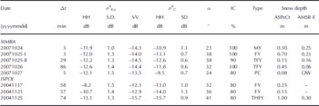
The discrepancies in snow depth between ASPeCt and AMSR-E shown in Table 1 (20071025-I and 20071026 as well as 20041125) should also not to be over-interpreted, as the variability in the ASPeCt snow depths is of course much higher than that of the AMSR-E snow depths (see Fig. 2 and 3). the snow depth of 1.0 m observed during ISPOL on 25 November (Table 1: 20041125) is a singular event in a series of much smaller snow depths of ~0.4m which agree within 0.15 m with AMSR-E snow depths (Fig. 3a). In contrast, snow depths of 0.70 and 0.45 m observed during SIMBA on 25 and 26 October (Table 1: 20071025-I and 20071026) seem to belong to an area where ASPeCt snow depths are continuously larger than the AMSR-E snow depth (Fig. 3d). This is also supported by Figure 2c and d: some of the average ASPeCt snow depths stand out clearly against the smaller AMSR-E snow depths in the background.

Figure 5a–c show an example of the remote-sensing datasets, on which the further analysis is based (see last paragraph of section 3): an ASAR image, a QuikSCAT σ0KuHH image and an AMSR-E snow depth map. the white rectangular frames in Figure 5b and c denote the region covered by the ASAR image. Note the difference in the location of the ice edge in Figure 5b compared to Figure 5a and c; this is caused by the fact that during this time the ice edge was advancing rapidly northwards. This process cannot be resolved with the 5 day (8–12 October) average AMSR-E snow depth shown in Figure 5b.

Fig. 5.

Example of involved datasets for 12 October 2007 SIMBA cruise. (a) ASAR WSM image acquired at 13:40 UTC; grid resolution 125 m; legend below the image. (b) AMSR-E snow depth at 12.5 km grid resolution; white, grey and black areas denote regions flagged as 150, land and open water, respectively; (c) QuikSCAT image at 12.5 km grid resolution; land is flagged grey. White rectangles in (b) and (c) mark the area covered by the SAR image shown in (a). (d) Histograms of and obtained at 12.5 km grid resolution within (a) and the white rectangle in (c). (e) Histograms of the Ku-band VV/HH polarization ratio together with histograms of the σ ⁰ standard deviation of same area as in (d). (f) Histogram of AMSR-E snow depth values within the rectangle in (b). (g) at 12.5 km grid resolution vs its standard deviation. (h) vs Values shown in (g) and (h) are scaled with the coincident AMSR-E snow depth within the respective gridcell. the number N (d–h) denotes the number of used ice-covered gridcells with at least 60% ice concentration.

The unimodal histogram shown in Figure 5d reveals modal values of –15.5 and –13.6 dB for VV- and HH-polarization, respectively, and a modal value of –12.0 dB (see Reference Ozsoy-Cicek, Kern, Ackley, Xie and TekeliOzsoy-Cicek and others, in press). the histograms given in Figure 5e reveal that Ku-band VV-/HH-polarization ratio values tend to be normally distributed across the ice-covered part of the image (modal value –2.3 dB). the standard deviation is also normally distributed, while the standard deviation has a skewed distribution with almost three modes: 1.0 and 2.0 dB (and 0.6 dB). This distribution is caused by the presence of different ice types: fast ice, drift ice and the marginal ice zone (MIZ) which stands out clearly in Figure 5a at ~68^˚ S. Averaging the 125 m grid resolution ASAR image over 12.5 km in a region with radar backscatter values that vary by 10 dB over the scale of ~1 km, as in the MIZ, causes the mentioned mode of high standard deviations in Figure 5e. the areal extent of the fast ice cover in our region of interest is rather small. From visual inspection of the full SIMBA dataset standard deviation maps (not shown), we know that the majority of the observed low standard deviations originate from a narrow zone of a very uniform radar backscatter signature. This zone is found between the MIZ and drift ice closer to the coast (see Fig. 5d, close to, east and west of Peter I Island situated at 69^˚ S, 90.5^˚ W). This zone most likely comprises first-year ice with floe sizes ~50–100m and a quite substantial snow cover of up to 0.45m (Table 1: 20071026; Reference Ozsoy-Cicek, Kern, Ackley, Xie and TekeliOzsoy-Cicek and others, in press).

Figure 5f shows the snow depth distribution; it has two modes. One is situated at ~0 cm which is the new ice forming in the MIZ, and in the polynyas adjacent to the coast (Fig. 5a). This mode is absent until about 9 October but afterwards shows the highest or at least the second highest probability because of the increasing new ice fraction due to the ice edge advance. the second mode, situated at ~0.2 m, is present during the entire SIMBA period, and decreases towards the end of October. Finally, there is evidence for a third mode comprising higher snow depths (0.35 m).

Figure 5g and h display the aforementioned scatter plots (see last paragraph of section 3), and reveal some clustering of (mean and standard deviation) values with AMSR-E snow depth values (Fig. 5g), as does the combination of and (Fig. 5h). We revisit these two combinations later.

In Figure 6 we look at the general development of the mean AMSR-E snow depth (Fig. 6a and d) in comparison to the mean values of σ0KuHH, σ0KuVV and σ0CHH (Fig. 6b and e) for the SIMBA period. Mean snow depths in regions PETERIA_ASC and PETERIA_DES decrease from an initial value of 0.20 m at the beginning of October to about 0.09 m on 10 November 2007. Time series derived for the other two ASAR image groups (not shown) are shorter but also reveal this decreasing trend.

Fig. 6.

Time series of the ASAR image area-averaged (only gridcells inside the ASAR image overlap masks, >60% ice concentration and situated north of 73^˚ S) snow depth (a, d), and and (b, e) for all available 3 day repeat-pass Envisat ASAR images of the regions PETERIA_DES (a, b) and PETERIA_ASC (d, e), locations of which are given in (c) and (f). Vertical bars denote one standard deviation. Gaps in the time series are caused by (1) ASAR images that were not acquired within the selected time slot of ±15 min (see section 3) or (2) ASAR images that cover too small a portion of the ASAR image overlap mask.

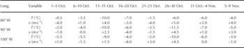
Mean tends to decrease by 1–2 dB (Fig. 6b and e). This gradual decrease could be caused by increased attenuation of microwave radiation in an, on average, increasingly wet snow cover. the increasing solar radiation at this time of year could be one driver for elevated snow wetness due to internal snowmelt, provided that clear-sky conditions prevail. Modelled air temperatures (Table 2) reveal that after a cold 5 day period (pentad) (26–30 October), air temperatures increased at the latitude of Peter I Island until the last pentad shown (4–9 November). on 10 November, air temperatures were between –1.5^˚C and –3^˚C, high enough to observe liquid water in snow on sea ice (e.g. Reference Garrity and CarseyGarrity, 1992). the Ku-band VV-/HH-polarization ratio stayed constant at ~2dB.

Table 2.

Mean 1000 hPa level air temperature and v-component of the wind speed at 69^˚ S and the given longitude as derived online using data of the operational US National Centers for Environmental Prediction (NCEP)/US National Center for Atmospheric Research (NCAR) weather forecasting model (http://www.esrl.noaa.gov/psd/data/histdata). Positive (negative) values of v denote a southerly (northerly) wind component

The mean σ ⁰CHH is almost constant and stays within the variability given by the error bars (one standard deviation) for region PETERIA_DES (Fig. 6b) but is more variable over time in the other region (Fig. 6e). the observed decrease in by 3 dB over a period of 12 days (Fig. 6e), and other variations in that are not further discussed here, can be assigned to changes in the mean distribution caused by the change from a compact to an open, divergent sea-ice cover. These changes can be identified in the SIMBA 2007 Envisat ASAR image dataset by interpreting the distributions of and its standard deviation. While a compact ice cover does not contain any leads and exhibits a compact ice edge, the open ice cover can contain lots of leads, a divergent ice edge and is additionally associated with polynya formation along the coast. Figure 5a shows an example of an open ice cover with the characteristic signature of dark and bright bands in the MIZ which indicate areas of new ice (low and pancake ice (high with a number of leads covered by new ice in the pack ice, and a polynya at the coast, also covered by new ice. the observed changes in the ice conditions and thus in can be related to changes in the mean wind direction, as can be deduced from Table 2 showing the meridional component of the modelled mean 5 day wind speed.

We chose region PETERIA_DES (Fig. 6c) for further investigation because it contains the largest number of different ice types – fast ice, polynya, pack ice and MIZ – and was investigated in the case study by Reference Ozsoy-Cicek, Kern, Ackley, Xie and TekeliOzsoy-Cicek and others (in press). Figure 7 shows versus scaled with AMSR-E snow depths (see Fig. 5g). the plots in Figure 7 reveal an elongated ‘cloud’ of - pairs with snow depths above ~0.2 m, which stretches along the red dashed line and can be tracked through almost all plots. There is evidence for a second elongated ‘cloud’ of - pairs with snow depths at or below 0.2 m. This stretches along the dashed black line and can also be tracked through almost all plots. In contrast to the aforementioned ‘cloud’ (red dashed line), this one is not very well defined, particularly in Figure 7a–c, and it shifts over time by 2–3 dB towards lower σ0KuHH values (cf. Fig. 7b).

Fig. 7.

Scatter plots of Vs for all 3 day repeat pass ASAR for region PETERIA_DES (see also Fig. 6a and b) between 3 October and 10 November 2007. All symbols are colour-coded according to the AMSR-E snow depth within the respective co-located gridcell. the map given in (k) denotes the location of region PETER1A_DES. Dashed red and black lines are shown to indicate a preferential alignment of data points along two ‘clouds’, which are referred to as STC and SHC in the text.

The ‘cloud’ with the steeper slope (steeply sloping cloud (STC)) covers a larger (smaller) range of () values, while the ‘cloud’ with the shallower slope (shallowly sloping cloud (SHC)) covers a smaller (larger) range of () values. the SHC extends into that range, which seems to be typical for the zone of rough cake-ice-like first-year ice south of the MIZ (Table 1: 20071026; Fig. 5a). We suggest that, with this ‘cloud’, rough first-year ice regions could be identified.

According to a case study carried out with data from 12 October 2007 (Reference Ozsoy-Cicek, Kern, Ackley, Xie and TekeliOzsoy-Cicek and others, in press), and occupy a rather narrow range (~2 dB) regardless of the ice type, while values occupy a wide range in the perennial ice region and in the MIZ. Our new results differ from these earlier findings, in that the range of especially in the STC (red dashed line, Fig. 7), is much larger (at least 5 dB). This is possibly due to a difference in selecting the data. In this study, we did not look at areas that, in accordance with coincident C-band SAR imagery, belong to specific ice types (Reference Ozsoy-Cicek, Kern, Ackley, Xie and TekeliOzsoy-Cicek and others, in press) but rather examined the entire ice-covered area within the colocated ASAR image (Fig. 3a and c). the STC tends to be associated with, on average, larger snow depths than the SHC (see above), and average values are relatively low, i.e. about –14 dB. We suggest therefore that the STC may be associated with merely undeformed first- or second-year ice, the snow cover of which is subject to the onset of melt–refreeze cycles which can cause σ0KuHH to vary while remains stable.

The STC is relatively well defined but the SHC is not. Here actually two clouds do overlap, at least temporarily. One is caused by the expansion of the MIZ, starting after 6 October, and the other is the one that is visible before this expansion (Fig. 7b and c). We prepared a series of plots similar to that shown in Figure 7 for σ0CHH vs its standard deviation (not shown). We found that thin snow (<0.2 m) seems to be associated with high (~–12 dB), while thick snow (>0.2 m) seems to coincide with low (~–14 dB). However, at the same time, standard deviations are low, i.e. <0.8 dB, as would be typical for the zone of rough first-year ice discussed in the context of Figure 5e. As time progresses, the amount of data pairs with low standard deviations, high and snow depths below 0.15 m increases. According to the observations during the SIMBA outbound leg, this zone of rough first-year ice is potentially one of the regions where AMSR-E snow depths underestimate ASPeCt snow depths (Table 1). We found further that low AMSR-E snow depths, i.e. <0.05 m, are associated with the MIZ, particularly during ice-edge advance, as is evident from predominant high standard deviations (1.1–2.5 dB). By means of these findings we can distinguish two subsets of σ0KuHH–σ0CHH data pairs in the SHC. One exhibits a small standard deviation of <0.8 dB, and is thus associated with the aforementioned zone of rough first-year ice. the second exhibits high standard deviation (>1.5 dB), and is thus associated with the MIZ.