1. Introduction
Synthetic active particles are micron and submicron sized colloidal particles which can propel themselves along predictable trajectories. The self-propulsion arises from the generation of local concentration gradient at the surface, which is induced by variation in the surface activity such as absorption or reaction (Anderson Reference Anderson1989; Golestanian, Liverpool & Ajdari Reference Golestanian, Liverpool and Ajdari2005, Reference Golestanian, Liverpool and Ajdari2007; Jülicher & Prost Reference Jülicher and Prost2009). These active particles play an important role in biomedical research; they offer possible applications in drug-delivery micromachines and controlled studies of microbial infections through biosensing (Gao & Wang Reference Gao and Wang2014; Su et al. Reference Su, Price, Jing, Tian, Liu and Qian2019). Furthermore, a suspension of active particles represents a non-equilibrium system which exhibits characteristics such as enhanced fluid mixing in complex fluids (Gomez-Solano, Blokhuis & Bechinger Reference Gomez-Solano, Blokhuis and Bechinger2016) and inertialess turbulence, which are also observed in microbial suspensions and granular matter (Patteson, Gopinath & Arratia Reference Patteson, Gopinath and Arratia2016). Therefore, understanding such novel self-propelled systems provides insights which extend to a wide range of physical phenomena, making it intriguing from a scientific standpoint.
The notion of self-propulsion at the microscale was introduced via exploitation of electrochemical-mechanical transduction mechanism, i.e. conversion of electrochemical energy (stored in electrolytes) to power mechanical motion. Paxton et al. (Reference Paxton, Kistler, Olmeda, Sen, St. Angelo, Cao, Mallouk, Lammert and Crespi2004, Reference Paxton, Sundararajan, Mallouk and Sen2006) and Fournier-Bidoz et al. (Reference Fournier-Bidoz, Arsenault, Manners and Ozin2005) fabricated bimetallic microrods by coating the two halves with platinum and silver. When immersed in an aqueous solution of hydrogen peroxide, the oxidation process generates excess electrons and protons (H $^{+}$) at the platinum end. The electrons are transported to the other end through conduction, where they are consumed to reduce hydrogen peroxide. The asymmetric distribution of protons drives the autonomous motion of the microrod, which was later called ‘self-electrophoresis’.
Golestanian et al. (Reference Golestanian, Liverpool and Ajdari2005) and Howse et al. (Reference Howse, Jones, Ryan, Gough, Vafabakhsh and Golestanian2007) studied the second mechanism of self-propulsion: conversion of chemical energy (arising from molecular interactions such as van der Waals) to power the mechanical motion in a non-electrolytic medium. Golestanian et al. (Reference Golestanian, Liverpool and Ajdari2007) proposed the first continuum framework to understand the underlying mechanism which drives the self-propulsion of Janus spheres. On the basis of existing experimental studies (Fournier-Bidoz et al. Reference Fournier-Bidoz, Arsenault, Manners and Ozin2005; Golestanian et al. Reference Golestanian, Liverpool and Ajdari2005), three major assumptions were made: (i) the interaction layer of solute molecules is asymptotically thin in comparison to the particle radius ( $\epsilon \ll 1$, where
 $\epsilon$ is the ratio of the thickness of interaction layer to particle radius); (ii) the active (catalytic) surface absorbs (or desorbs) the solute molecules at a fixed rate and diffusion time scale is much shorter than the reactive time scale; and (iii) advective effects are negligible. Borrowing insights from the seminal works of Derjaguin et al. (Reference Derjaguin, Sidorenkov, Zubashchenkov and Kiseleva1947) and Anderson, Prieve and coworkers (Anderson, Lowell & Prieve Reference Anderson, Lowell and Prieve1982; Anderson Reference Anderson1989), they showed that the interaction between the particle and the solute molecules creates a pressure gradient inside the thin interaction layer. This pressure gradient is balanced by the viscous stresses which is the driving mechanism for self-propulsion. An external variation in solute concentration around the colloid can trigger the pressure gradient which generates a surface slip. Consequently, the freely suspended particle moves in the direction of chemical gradient, known as diffusiophoresis: a macroscale motion manifested through an asymmetry at the microscale. A Janus sphere (possessing a chemically active cap coated on an inert particle) can create and sustain this pressure gradient, as its asymmetrically active surface facilitates a tangential concentration gradient and is therefore also called a self-diffusiophoretic particle.
The continuum description assumes that the solute molecules do not occupy volume and therefore loses its validity for nanometre sized Janus spheres. For such cases, Córdova-Figueroa & Brady (Reference Córdova-Figueroa and Brady2008) and Brady (Reference Brady2011) provided a colloidal perspective to diffusiophoresis: solute molecule and particle interact both energetically (through hard-sphere and van der Waals forces) and hydrodynamically with each other. Later Sharifi-Mood, Koplik & Maldarelli (Reference Sharifi-Mood, Koplik and Maldarelli2013) demonstrated that the results derived by Brady (Reference Brady2011) (for diffusiophoretic velocity) can be obtained through a continuum description, in the limit of asymptotically small solute molecules. They relaxed the assumption of a thin interaction layer and incorporated the effects of an irreversible reaction (characterized by Damköhler number) at the active surface which was found to dampen the propulsion.
Michelin & Lauga (Reference Michelin and Lauga2014) explored the effects of finite advection on self-propulsion. They found that the particles exhibiting attractive interaction with solute molecules show a maxima in swimming speed at a finite Péclet number ( $Pe \sim O(1)$, here
 $Pe$ is the ratio of diffusive to advective time scales); whereas, for repulsive interactions, the swimming speed always reduces with increase in advection. In agreement with Sharifi-Mood et al. (Reference Sharifi-Mood, Koplik and Maldarelli2013), they also reported a monotonic decrease in swimming velocity with an increase in Damköhler number. Utilizing matched asymptotic expansions, they showed that the diffusive flux at the surface of the Janus sphere is equal to that at the outer edge of the interaction layer, provided
 $\epsilon Pe \ll 1$.
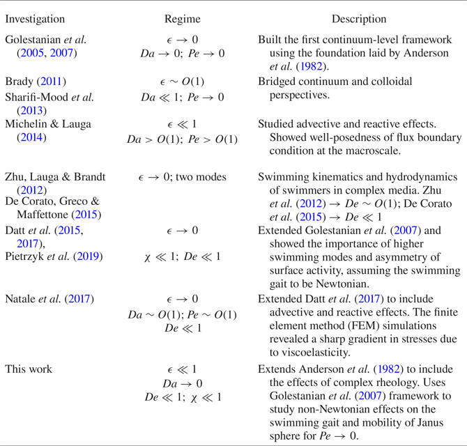
All the aforementioned studies assume the surrounding medium to be Newtonian. Since a majority of potential applications of the synthesized active particles lie in drug-delivery and other areas of biological research (Patteson et al. Reference Patteson, Gopinath and Arratia2016; Su et al. Reference Su, Price, Jing, Tian, Liu and Qian2019), understanding the influence of complex rheology on self-propulsion is essential. There has been limited progress towards this, both experimentally and theoretically. Table 1 summarizes the theoretical studies which analysed self-propulsion in various regimes. The experimental and theoretical analysis of Gomez-Solano et al. (Reference Gomez-Solano, Blokhuis and Bechinger2016) and Aragones, Yazdi & Alexander-Katz (Reference Aragones, Yazdi and Alexander-Katz2018) demonstrated that the translational swimming of a Janus particle is coupled to the rotational motion in a viscoelastic medium. Recently, Saad & Natale (Reference Saad and Natale2019) studied the effect of polymer entanglements on active motion and showed that the particle can escape the entangled confinements at time scales significantly shorter than the polymer relaxation time.
A summary of continuum-level studies in the past towards the modelling of a non-Brownian active particle; the first section of the table describes the studies in Newtonian medium in various regimes and the second section summarizes the studies which explored the effects of non-Newtonian behaviour. Here,  $\epsilon$ is the interaction layer thickness, normalized by the particle radius;
 $Da$ is the Damköhler number which represents the ratio of time scale associated with diffusion to that of reaction;
 $Pe$ is the Péclet number which is the ratio of time scale associated with diffusion to that of advection;
 $De$ is the Deborah number which governs the ratio of time scale of polymer relaxation to that of advection; and
 $\chi$ represents the deviation of infinite shear rate viscosity from that of zero shear rate (the difference is normalized with the infinite shear rate viscosity).

There have been a few theoretical studies in the past which have used the continuum-level framework and studied the effect of bulk non-Newtonian stresses on active propulsion. Zhu et al. (Reference Zhu, Lauga and Brandt2012) employed the Giesekus model to study squirming in a viscoelastic fluid, considering the first two modes of swimming. They reported that swimming speed (and the swimming power required) is always lower than that in Newtonian fluids, with a minimum at a moderate value of Weissenberg number. Using a second-order fluid model, De Corato et al. (Reference De Corato, Greco and Maffettone2015) also studied locomotion of a two-mode squirmer. They reported that ‘pullers’ are slowed, ‘pushers’ are hastened and ‘neutral’ squirmers are unaffected in weakly viscoelastic fluids. Later Datt et al. (Reference Datt, Zhu, Elfring and Pak2015) showed that it is essential to consider higher modes while modelling squirmers in a non-Newtonian medium as the constitutive equation is nonlinear. Using a Carreau–Yasuda model, they demonstrated that the swimming may be faster or slower in shear-thinning fluids (compared with Newtonian fluids) depending upon the rate of actuation, i.e. strength of the swimming modes. Their subsequent study (Datt et al. Reference Datt, Natale, Hatzikiriakos and Elfring2017) extended the analysis of Golestanian et al. (Reference Golestanian, Liverpool and Ajdari2007) to understand the self-propulsion of a Janus sphere in complex media. Through an approach based on the reciprocal theorem, they analysed the effect of bulk non-Newtonian stresses on the swimming velocity, assuming a prescribed slip velocity. They found: (i) swimming is always slower in weakly shear-thinning fluids; and (ii) for weakly viscoelastic fluid, a Janus sphere swims faster if surface coverage of activity is more than half ( ${>} {\rm \pi} /2$) and viceversa. However, they have acknowledged that the assumption of Newtonian slip in a non-Newtonian medium may not hold true. A change in slip velocity may significantly alter self-propulsion and therefore requires further investigation. A recent study by Natale et al. (Reference Natale, Datt, Hatzikiriakos and Elfring2017) extended the work of Datt et al. (Reference Datt, Natale, Hatzikiriakos and Elfring2017) to investigate the effects of advection and reaction (i.e. finite Péclet and Damköhler numbers) on self-diffusiophoresis through complex media. Their FEM simulations demonstrated the presence of an extensional flow across the point of discontinuity in the surface activity. This behaviour was triggered due to large gradients in viscoelastic stresses. The origin of these viscoelasticity-triggered extensional flows is currently unknown. Given the recent interest in self-propulsion through complex medium with several open questions in the literature (Datt et al. Reference Datt, Natale, Hatzikiriakos and Elfring2017; Natale et al. Reference Natale, Datt, Hatzikiriakos and Elfring2017; Pietrzyk et al. Reference Pietrzyk, Nganguia, Datt, Zhu, Elfring and Pak2019), it is natural to ask: How does the slip change in complex fluids and what is its relationship to the concentration field?
The importance of considering non-Newtonian effects in the thin interaction region around a diffusiophoretic particle can be realized by considering the progress in the field of electrophoresis. Khair, Posluszny & Walker (Reference Khair, Posluszny and Walker2012) demonstrated that the modification in slip due to shear-thinning can alter the mobility of an electrophoretic particle and the flow field around it. Very recently, through the use of various continuum-level rheological models (Oldroyd-B, Giesekus, FENE-P, and FENE-CR), Li & Koch (Reference Li and Koch2020) showed that the electrophoretic particle (similar to a neutral squirmer in Newtonian fluid) behaves like a puller-type squirmer at low Weissenberg numbers. Such behaviour arises primarily due to the elastic effects in the thin electrical double layer. These studies show that the high shear rate inside the thin layer generates significant polymer extension and deformation which needs to be accounted for in the prediction of phoretic motion. Motivated by these recent developments in the context of electrophoresis (Khair et al. Reference Khair, Posluszny and Walker2012; Zhao & Yang Reference Zhao and Yang2013; Li & Koch Reference Li and Koch2020), we aim to investigate the modification due to complex rheology in both the slip and mobility of a self-propelling active particle.
In this work, we study the influence of viscoelasticity (second-order fluid model) and shear-thinning (Carreau-fluid model) on the slip and mobility of an axisymmetric Janus particle. Using matched asymptotic expansions, we provide an analytical expression for the modification of the diffusio-osmotic slip due to complex rheology. Employing the reciprocal theorem, we evaluate the modification in the swimming velocity. Our results are applicable to a general diffusio-osmotic flow of complex fluid and hence can be used to model the transport of biological fluids through narrow channels and confinements, where applying a pressure drop is undesirable (Michelin et al. Reference Michelin, Montenegro-Johnson, De Canio, Lobato-Dauzier and Lauga2015; Lisicki, Michelin & Lauga Reference Lisicki, Michelin and Lauga2016; Michelin & Lauga Reference Michelin and Lauga2019).
2. Active particle in a second-order fluid
We consider an active particle surrounded by a non-Newtonian fluid medium consisting of a solute at uniform concentration  $C_{\infty }^{*}$. The solute, treated as a continuum, interacts with the active particle of radius
 $a^{*}$. The short-range interaction potential is governed by
 \begin{equation} \mathcal{P}^{*}(r,\theta)=k_{B}^{*} T^{*} \psi(r,\theta) , \end{equation}
which acts over the length scale corresponding to the interaction layer thickness ( $\lambda _{I}^{*})$, where
 $\lambda _{I}^{*} \ll a^{*}$. Here
 ${*}$ denotes the dimensional variables and
 $\psi$ is interaction potential energy between the solute molecules and particle surface, scaled with the thermal energy (
 $k_{B}^{*} T^{*}$). This interaction generates a pressure field in the thin interaction layer, which decays to zero far away from the surface. The particle surface is partially active; a fixed-rate absorptive flux (
 $\mathcal {A}^{*}$) varies as a step function in the tangential direction. Since the interaction layer (
 $\lambda _{I}^{*}$) is very thin compared with the particle radius (
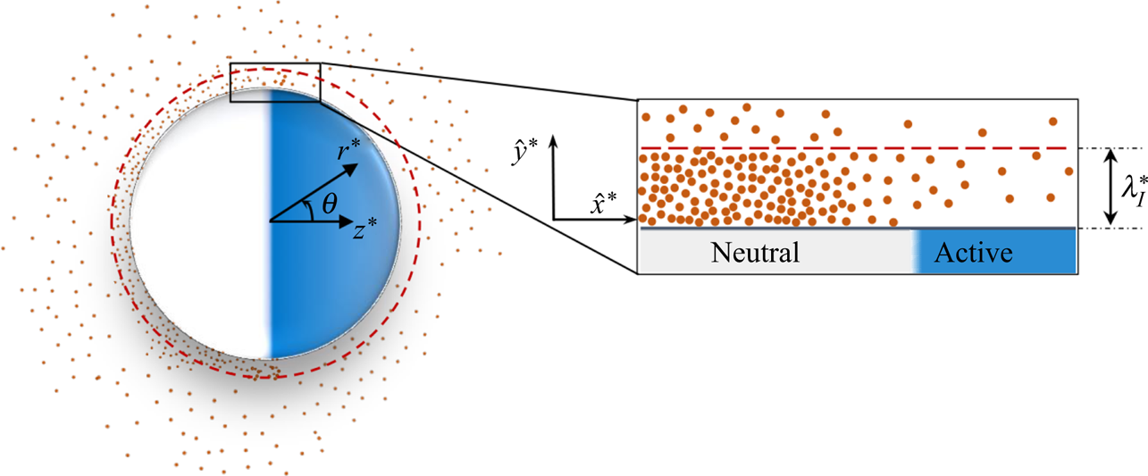
 $a^{*}$), we model this as a diffusio-osmotic flow over a flat surface (see figure 1). This approximation neglects the curvature effects and introduces an error of
 ${O}(\lambda _{I}^{*}/ a^{*})$, and has been employed earlier in studies involving particle electrophoresis (O'Brien Reference O'Brien1983; Anderson Reference Anderson1989).
Schematic of an axisymmetric Janus particle suspended in a non-Newtonian medium with uniform external solute concentration. Zoomed in view shows the solute in the thin interaction layer above a surface with varying activity. Here,  $\lambda _{I}^{*}$ is the interaction layer thickness.

We assume the rheology inside and outside the interaction layer to follow the second-order fluid (SOF) model (Bird, Armstrong & Hassager Reference Bird, Armstrong and Hassager1987). This assumption is valid for slow and weakly non-Newtonian flows, i.e. polymers with low molecular weight ( ${\sim }10^{4}$) and radius of gyration smaller than the interaction layer thickness which is typically
 $1\text {--}10\ \textrm {nm}$ (Sharifi-Mood et al. Reference Sharifi-Mood, Koplik and Maldarelli2013). The qualitative insights obtained through such continuum models can also be extended to the cases of larger polymers as their segments would experience strong shear, which can result in modification of the dynamics in the interaction layer (Li & Koch Reference Li and Koch2020). We also assume the solute molecules, inside and outside the interaction layer, to follow Fickian diffusion with constant diffusivity. It has been reported that the presence of polymers significantly affects the diffusive mass transport in a stagnant polymeric medium (Maldonado-Camargo & Rinaldi Reference Maldonado-Camargo and Rinaldi2016; Makuch et al. Reference Makuch, Hołyst, Kalwarczyk, Garstecki and Brady2020). To our knowledge, there has been no study conducted on the mass transport in sheared complex flows. As a first step, we focus on gaining qualitative insights and assume that the solute molecules and polymers are in the dilute concentration regime and the associated effects, such as volume exclusion and variable diffusivity, do not affect the system at leading order.
Following Anderson et al. (Reference Anderson, Lowell and Prieve1982) and Michelin & Lauga (Reference Michelin and Lauga2014), we represent the system using the following non-dimensional equations:
 \begin{gather} \boldsymbol{\nabla} \boldsymbol{\cdot} \boldsymbol{u}=0, \quad -\boldsymbol{\nabla} p + \nabla^{2}\boldsymbol{u}+De \, \boldsymbol{\nabla} \boldsymbol{\cdot} \boldsymbol{\mathsf{S}} -\frac{1}{\epsilon^{2}} (c+C_{\infty})\boldsymbol{\nabla} \psi=\boldsymbol{0}, \end{gather}
 \begin{gather} Pe(\boldsymbol{u}\boldsymbol{\cdot} \boldsymbol{\nabla} c)=\boldsymbol{\nabla} \boldsymbol{\cdot} [ \boldsymbol{\nabla} c + \left( c+C_{\infty}\right) \boldsymbol{\nabla} \psi ] . \end{gather}
The characteristic scales are
 \begin{equation} C_{ch}=\frac{|\mathcal{A^{*}}|a^{*}}{D^{*}}, \; U_{ch}=\frac{k^{*}_{B}T^{*}\lambda_{I}^{* \, 2} C_{ch}}{\mu^{*} a^{*}},\; p_{ch}=\frac{\mu^{*} U_{ch}}{a^{*}},\; y_{ch}=x_{ch}=a^{*}. \end{equation}
Here,  $D^{*}$ is the solute diffusion coefficient,
 $|\mathcal {A}^{*}|$ is the maximum magnitude of activity,
 $c$ denotes the disturbance to the uniform concentration
 $C_{\infty }$ (defined as
 $c=C-C_{\infty }$). In (2.2a), the polymeric stress
 $\boldsymbol{\mathsf{S}}=\boldsymbol{\mathsf{A}} \boldsymbol{\cdot} \boldsymbol{\mathsf{A}} + \delta \boldsymbol{\mathsf{B}}$, where
 $\boldsymbol{\mathsf{A}}$ is the rate of strain tensor (
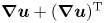 $\boldsymbol {\nabla } \boldsymbol {u} + (\boldsymbol {\nabla } \boldsymbol {u})^{\rm T}$) and
 $\boldsymbol{\mathsf{B}}$ is the steady-state Rivlin–Ericksen tensor (covariant derivative of rate of strain tensor
 $\boldsymbol{\mathsf{A}}$) (Bird et al. Reference Bird, Armstrong and Hassager1987),
 \begin{equation} \boldsymbol{\mathsf{B}} = \boldsymbol{U} \boldsymbol{\cdot} \boldsymbol{\nabla} \boldsymbol{\mathsf{A}} + \boldsymbol{\mathsf{A}}\boldsymbol{\cdot} \boldsymbol{\nabla} \boldsymbol{U}^{\rm T} + \boldsymbol{\nabla} \boldsymbol{U} \boldsymbol{\cdot} \boldsymbol{\mathsf{A}}. \end{equation}
where  ${\rm T}$ denotes the transpose. The dimensionless quantities are defined as
 \begin{equation} Pe=\frac{U_{ch}a^{*}}{D^{*}}, \; De=\frac{\Psi_{1}^{*}+\Psi_{2}^{*}}{\mu^{*}}\left( \frac{U_{ch}}{a^{*}}\right), \; \delta=\frac{-\Psi_{1}^{*}}{2\left(\Psi_{1}^{*}+\Psi_{2}^{*} \right) } \ \text{and} \ \epsilon=\frac{\lambda_{I}^{*}}{a^{*}}, \end{equation}
where  $Pe$ (Péclet number) is the ratio of diffusive to advective time scales,
 $De$ (Deborah number) is defined as the ratio of viscoelastic time scale to that based on shear arsing due to macroscale movement of the Janus sphere,
 $\delta$ is a viscometric parameter which compares first and second normal stress coefficients (
 $\Psi _{1}^{*}$ and
 $\Psi _{2}^{*}$, respectively) and
 $\epsilon$ is the dimensionless thickness of the interaction layer.
The boundary conditions are
 \begin{gather} \left( \left.\frac{\partial c}{\partial y}\right\vert_{y=0} +\left.(c+C_{\infty}) \frac{\partial \psi}{\partial y}\right\vert_{y=0} \right) = \frac{\mathcal{A^{*}}(x)}{|\mathcal{A^{*}}|}=\mathcal{K}(x)\quad \text{and}\quad \boldsymbol{u}= \boldsymbol{0} \quad \text{at } y=0\ , \end{gather}
 \begin{gather} p \rightarrow 0 ,\ \psi \rightarrow 0 \quad \text{and}\quad c \rightarrow 0 \quad \text{as } y\rightarrow \infty. \end{gather}
In the next sections, we investigate the influence of non-Newtonian effects on the diffusio-osmotic slip on a partially active surface using matched asymptotic expansions (MAE).
2.1. Evaluation of the diffusio-osmotic slip
For an asymptotically thin interaction region ( $\epsilon \ll 1$), we expand the field variables (
 $\boldsymbol {u},c, p, \psi$) as
 \begin{equation} f(x,y)=f^{(0)}(x,y)+\epsilon f^{(1)}(x,y)+\cdots. \end{equation}
Following Michelin & Lauga (Reference Michelin and Lauga2014), we divide the domain into an ‘inner’ ( $0 \ll y \ll 1$) and ‘outer’ region (
 $y \gg 1$). We use MAE to replace the solution of the inner region with coarse-grained boundary conditions for the outer region.
2.1.1. Outer region
Neglecting the rapidly decaying interaction potential in the outer region, i.e.  $\psi =0$ (Sharifi-Mood et al. Reference Sharifi-Mood, Koplik and Maldarelli2013; Michelin & Lauga Reference Michelin and Lauga2014), the leading-order equations read
 \begin{gather} \boldsymbol{\nabla} \boldsymbol{\cdot} \boldsymbol{u}^{(0)} = 0, \quad - \boldsymbol{\nabla} p^{(0)} + {\nabla}^{2} \boldsymbol{u}^{(0)} + De \, \boldsymbol{\nabla} \boldsymbol{\cdot} \boldsymbol{\mathsf{S}}^{(0)} = \boldsymbol{0}, \end{gather}
 \begin{gather} Pe(\boldsymbol{u}^{(0)}\boldsymbol{\cdot} \boldsymbol{\nabla} c^{(0)})= {\nabla}^{2}c^{(0)}, \end{gather}
subject to the following boundary conditions:
 \begin{gather} \boldsymbol{u}^{(0)} \rightarrow \boldsymbol{0} , \; p^{(0)} \rightarrow 0 \quad \text{and}\quad c^{(0)} \rightarrow 0 \quad \text{as } y \rightarrow \infty, \end{gather}
 \begin{gather} \boldsymbol{n}\boldsymbol{\cdot} \boldsymbol{\nabla} c^{(0)} = \mathcal{K}(x) \quad \text{at } y \rightarrow 0. \end{gather}
The concentration boundary condition (2.9b) has been shown to be well-posed, provided  $\epsilon Pe\ll 1$ (Michelin & Lauga Reference Michelin and Lauga2014, p. 580). To obtain the macroscale boundary condition for velocity at the surface (i.e.
 $y \rightarrow 0$), the outer solution must be matched with the inner solution.
2.1.2. Inner region
We first rescale the variables to derive the equations in the inner layer. The variables in the inner layer are defined as  $\hat {f}$. In the thin interaction layer limit (
 $\epsilon \ll 1$), using boundary layer principles, we define the characteristic scales for
 $y^{*}$-direction, vertical velocity (
 $v^{*}$) and pressure (
 $p^{*}$) as
 $\lambda _{I}^{*}$,
 $\epsilon \, U_{ch}$ and
 $p_{ch} \, \epsilon ^{-2}$, respectively. Using (2.7) and (2.2), we obtain the leading-order equations in the inner region as
 \begin{gather} \frac{\partial \hat{u}^{(0)}}{\partial \hat{x}} + \frac{\partial \hat{v}^{(0)}}{\partial \hat{y}} =0 , \end{gather}
 \begin{gather} - \frac{\partial \hat{p}^{(0)}}{\partial \hat{x}} + \frac{\partial^2 \hat{u}^{(0)}}{\partial \hat{y}^2} +De \left( \frac{\partial \hat{S}_{xx}^{(0)}}{\partial \hat{x}} + \frac{\partial \hat{S}_{yx}^{(0)}}{\partial \hat{y}} \right) = (\hat{c}^{(0)} + C_{\infty})\frac{\partial \hat{\psi}^{(0)}}{\partial \hat{x}} , \end{gather}
 \begin{gather} - \frac{\partial \hat{p}^{(0)}}{\partial \hat{y}} + De \left( \frac{\partial \hat{S}_{yy}^{(0)}}{\partial \hat{y}} \right) = (\hat{c}^{(0)}+C_{\infty}) \frac{\partial \hat{\psi}^{(0)}}{\partial \hat{y}} , \end{gather}
 \begin{gather} \epsilon^{2}Pe \left( \hat{u}^{(0)} \frac{\partial \hat{c}^{(0)}}{\partial \hat{x}} + \hat{v}^{(0)} \frac{\partial \hat{c}^{(0)}}{\partial \hat{y}} \right) = \frac{\partial}{\partial \hat{y}} \left( \frac{\partial \hat{c}^{(0)}}{\partial \hat{y}} + (\hat{c}^{(0)}+C_{\infty}) \frac{\partial \hat{\psi}^{(0)}}{\partial \hat{y}} \right) , \end{gather}
subject to the following surface boundary conditions at the leading order:
 \begin{equation} \left. \boldsymbol{u}^{(0)} \right\vert_{\hat{y}=0} = \boldsymbol{0} \quad \text{and}\quad \left( \left.\frac{\partial \hat{c}^{(0)}}{\partial \hat{y}}\right\vert_{\hat{y}=0} +\left.(\hat{c}^{(0)}+C_{\infty}) \frac{\partial \psi}{\partial \hat{y}}\right\vert_{\hat{y}=0} \right) =0. \end{equation}
For low to moderate advective effects (i.e.  $Pe \ll \epsilon ^{-2}$), we can neglect the left-hand side of (2.10d). This decouples the solute concentration field from the hydrodynamics. The pressure scaling in the inner region suggests a decay condition as
 $\hat {y} \rightarrow \infty$ (Michelin & Lauga Reference Michelin and Lauga2014, p. 579). The components of the polymeric stress tensor (
 $\boldsymbol{\mathsf{S}}$) are rescaled as
 \begin{gather} {\mathsf S}_{xx} = \frac{\hat{{\mathsf S}}_{xx}}{\epsilon^{2}} =\frac{1}{ \epsilon^{2}}\left( \frac{\partial \hat{u}}{\partial \hat{y}} \right)^{2},\quad {\mathsf S}_{yy} =\frac{\hat{{\mathsf S}}_{yy}}{\epsilon^{2}} =\frac{1}{\epsilon^{2}} \left( 1 +2 \delta \right) \left( \frac{\partial \hat{u}}{\partial \hat{y}} \right)^{2}, \end{gather}
 \begin{gather} {\mathsf S}_{xy}={\mathsf S}_{yx} = \dfrac{\hat{{\mathsf S}}_{xy}}{\epsilon} =\dfrac{\hat{{\mathsf S}}_{yx}}{\epsilon} =\dfrac{2 \delta}{ \epsilon}\left( \dfrac{\partial \hat{u}}{\partial \hat{y}} \dfrac{\partial \hat{u}}{\partial \hat{x}} + \dfrac{\hat{v} \dfrac{\partial^2 \hat{u}}{\partial \hat{y}^2} + \hat{u} \dfrac{\partial^2 \hat{u}}{\partial \hat{y} \partial \hat{x}} }{2} \right). \end{gather}
We now perform a perturbation expansion in Deborah number ( $De$), i.e. accounting for weakly nonlinear viscoelastic effects such that
 $\epsilon \ll De \ll 1$. The field variables for each term in (2.7) can be further expanded as
 \begin{equation} f^{(i)}(x,y)=f^{(i)}_{0}(x,y)+De \, f^{(i)}_{1}(x,y)+\cdots. \end{equation}
Here,  $f$ represents the velocity and pressure field. The concentration field is not expanded in
 $De$ as it is decoupled from velocity field in the inner region.
 ${O}$(
 $De^{0}$) solution: Since our objective is to obtain a first-order correction to the diffusio-osmotic slip, for convenience, we temporarily drop the superscript
 $(0)$ from all the variables. The solution to leading-order (i.e.
 $O$(
 $De^{0}$)) governing equations is obtained as
 \begin{equation} \hat{c}(\hat{x},\hat{y})=\mathcal{I}(\hat{x}) {\rm e}^{-\hat{\psi}(\hat{x},\hat{y})} - C_{\infty} , \quad \hat{p}_{0}(\hat{x},\hat{y})=\mathcal{I}(\hat{x}) \left( {\rm e}^{-\hat{\psi}(\hat{x},\hat{y})} -1 \right), \end{equation}
and
 \begin{equation} \hat{u}_{0}(\hat{x},\hat{y})=-\mathcal{I}'(\hat{x}) \int_{0}^{\hat{y}} \int_{t}^{\infty} \left( {\rm e}^{-\hat{\psi}(\hat{x},s)} -1 \right) {\textrm{d}}s \, {\textrm{d}}t + \mathcal{J}_{0}(\hat{x})\,\hat{y}. \end{equation}
Here,  $\mathcal {I}(\hat {x})$ and
 $\mathcal {J}_{0}(\hat {x})$ are to be determined through matching, and
 $\mathcal {I}'(\hat {x})$ represents
 ${\textrm {d}} \mathcal {I}/{\textrm {d}} {\hat {x}}$. The leading-order velocity field (
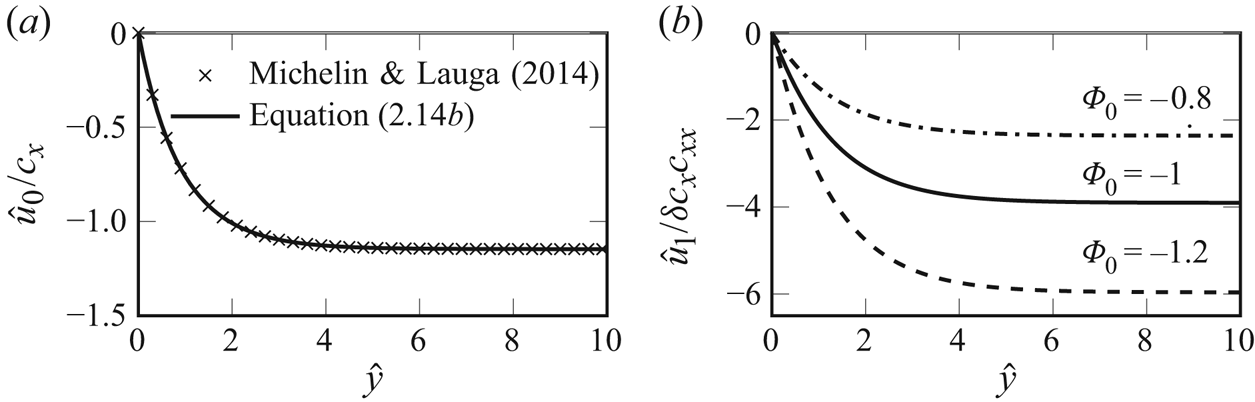
 $\hat {u}_{0}$) is represented in a form different from that reported by Anderson et al. (Reference Anderson, Lowell and Prieve1982) and Michelin & Lauga (Reference Michelin and Lauga2014), as it helps in the evaluation of the higher-order velocity field. It can be seen in figure 2(a) that this expression is equivalent to that provided in the literature.
(a) Velocity field of Newtonian fluid inside the interaction layer (for  $\Phi _{0}=-1$). (b) Variation of the modification to the velocity field. The results are for an exponentially decaying solute-surface interaction (
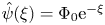 $\hat {\psi }(\xi )=\Phi _{0} {\rm e}^{-\xi }$), where a negative
 $\Phi _{0}$ represents an attractive interaction. Here,
 $c_{x}$ and
 $c_{xx}$ are the concentration gradients at the outer edge of the inner region i.e.
 $c_{x}\vert _{y=0}$ and
 $c_{xx}\vert _{y=0}$.

 ${O}$(
 $De^{1}$) solution: For ease of calculation, we assume the interaction potential (
 $\hat {\psi }$) to be independent of the tangential direction (
 $x$). The flow field at
 ${O}(De)$ is governed by
 \begin{gather} \frac{\partial \hat{u}_{1}}{\partial \hat{x}} + \frac{\partial \hat{v}_{1}}{\partial \hat{y}} =0 , \end{gather}
 \begin{gather} - \frac{\partial \hat{p}_{1}}{\partial \hat{x}} + \frac{\partial^2 \hat{u}_{1}}{\partial \hat{y}^2} + \frac{\partial \hat{S}_{xx \, 0}}{\partial \hat{x}} + \frac{\partial \hat{S}_{xy \, 0}}{\partial \hat{y}} = 0 , \end{gather}
 \begin{gather} - \frac{\partial \hat{p}_{1}}{\partial \hat{y}} + \frac{\partial \hat{S}_{yy \, 0}}{\partial \hat{y}} = 0. \end{gather}
Using the pressure decay condition ( $\hat {p} \rightarrow 0$ as
 $\hat {y} \rightarrow \infty$), the solution to (2.15c) yields
 $\hat {p}_{1}=\hat {S}_{yy \, 0} - \mathcal {J}_{0}(\hat {x})^{2}(1+2\delta )$. Simplifying (2.15b), we obtain
 \begin{align} \frac{\partial^{2} \hat{u}_{1}}{\partial \hat{y}^{2}} = - \delta \left\{ -\frac{\partial \hat{u}_{0}}{\partial \hat{y}} \frac{\partial^{2} \hat{u}_{0}}{\partial \hat{y} \partial \hat{x}} + \frac{\partial \hat{u}_{0}}{\partial \hat{x}} \frac{\partial^{2} \hat{u}_{0}}{\partial \hat{y}^{2}} + \hat{v}_{0} \frac{\partial^{3} \hat{u}_{0}}{\partial \hat{y}^{3}} + \hat{u}_{0} \frac{\partial^{3} \hat{u}_{0}}{\partial \hat{x} \partial \hat{y}^{2}} \right\} - 2 \mathcal{J}_{0}(\hat{x}) \mathcal{J}_{0}'(\hat{x}) (1+2\delta) . \end{align}
Here,  $\hat {v}_{0}$ is found by substituting (2.14b) in the continuity equation and integrating it over the
 $\hat {y}$ direction. Substituting (2.14b) and
 $\hat {v}_{0}$ into (2.16), integrating twice over the
 $\hat {y}$ direction and using the no-slip condition, we obtain
 \begin{align} \hat{u}_{1}&= \mathcal{J}_{1}(\hat{x}) \hat{y} - \delta \mathcal{I}'(\hat{x})\mathcal{I}''(\hat{x}) \int_{0}^{\hat{y}}\, \textrm{d}p \int_{p}^{\infty} \left\{ \left( \int_{r}^{\infty} \mathcal{F}(s) \, {\textrm{d}}s \right)^{2}\right.\nonumber\\ & \quad + \left. 2 \mathcal{F}(r) \left( \int_{0}^{r}s\mathcal{F}(s)\, {\textrm{d}}s + r \int_{r}^{\infty} \mathcal{F}(s)\, {\textrm{d}}s \right)\, {\textrm{d}}r \right. \nonumber\\ &\quad + \left. \hat{\psi}'(r) {\rm e}^{-\hat{\psi}(r)} \left( \int_{0}^{r} \left( r - \frac{s}{2} \right)s\mathcal{F}(s)\, {\textrm{d}}s \, + \frac{r^{2}}{2} \int_{r}^{\infty} \mathcal{F}(s)\, {\textrm{d}}s \right) \right. \nonumber\\ & \quad - \left. \left( \frac{\mathcal{J}_{0}(\hat{x})}{\mathcal{I}'(\hat{x})} + \frac{\mathcal{J}_{0}'(\hat{x})}{\mathcal{I}''(\hat{x})} \right) \left( r \mathcal{F}(r) + \int_{r}^{\infty} \mathcal{F}(s)\, \textrm{d}s \right) \right. \nonumber\\ &\quad + \left.\frac{\mathcal{J}_{0}(\hat{x})}{\mathcal{I}''(\hat{x})} \mathcal{F}'(r) \frac{r^{2}}{2} + \frac{\mathcal{J}_{0}(\hat{x}) \mathcal{J}_{(0)}'(\hat{x})}{\mathcal{I}'(\hat{x}) \mathcal{I}''(\hat{x})} - \frac{2\mathcal{J}_{0}(\hat{x}) \mathcal{J}_{0}'(\hat{x})(1+2\delta) }{\delta \mathcal{I}'(\hat{x}) \mathcal{I}''(\hat{x})} \right\} \,\textrm{d}r . \end{align}
Here,  $\mathcal {F}(\xi )=-1+{\rm e}^{-\hat {\psi }(\xi )}$,
 $\mathcal {J}_{0},\, \mathcal {J}_{1}$ and
 $\mathcal {I}$ are to be determined through matching. Details of the derivation can be found in the supplementary material available at https://doi.org/10.1017/jfm.2020.428.
2.1.3. Matching
For any field variable  $f$, the matching condition at
 ${O}$(
 $\epsilon ^{0}$) is
 \begin{equation} \lim_{y \rightarrow 0} \left(f^{(0)}_{0}+De f^{(0)}_{1}+\cdots\right)=\lim_{\hat{y} \rightarrow \infty}\left(\hat{f}^{(0)}_{0}+De \hat{f}^{(0)}_{1}+\cdots\right). \end{equation}
The matching condition for the concentration field ( $\hat {c}$) yields
 $\mathcal {I}(\hat {x}) = \lim _{y \rightarrow 0} c^{(0)}(x,y) + C_{\infty }$. We substitute (2.14b) and (2.17) in the above matching condition and obtain
 $\mathcal {J}_{0} = \mathcal {J}_{1}=0$ at the leading order. At the present order of approximation, the total slip velocity at the outer edge of the interaction layer is
 \begin{equation} \left. u^{(0)} \right\vert_{y=0} = \left. c^{(0)}_{x}\right\vert_{y=0} \left( M_{0} + De \, \delta \, M_{1} \left.c^{(0)}_{xx}\right\vert_{y=0} \right), \end{equation}
where  $M_{0}$ and
 $M_{1}$ are the mobility coefficients representing the Newtonian and non-Newtonian contribution, respectively,
 \begin{equation} M_{0} = - \int_{0}^{\infty} \int_{t}^{\infty} \mathcal{F}(s) \,\textrm{d}s \, \textrm{d}t \quad \text{and}\quad {M_{1}} = - {\displaystyle\int_{0}^{\infty} } \int_{p}^{\infty} \mathcal{G}(r)\, {\textrm{d}}r \, {\textrm{d}}p , \end{equation}
where
 \begin{align} \mathcal{G}(r)&= \left\{ \left( \int_{r}^{\infty} \mathcal{F}(s) \, {\textrm{d}}s \right)^{2} + 2\,\mathcal{F}(r) \left( \int_{0}^{r} s \mathcal{F}(s)\, {\textrm{d}} s + r \int_{r}^{\infty} \mathcal{F}(s)\, {\textrm{d}} s \right) \right. \nonumber\\ & \quad + \left. \hat{\psi}'(r) \, {\rm e}^{-\hat{\psi}(r)} \left( \int_{0}^{r} \left( r - \frac{s}{2}\right) s\, \mathcal{F}(s) \,{\textrm{d}}s + \frac{r^{2}}{2} \int_{r}^{\infty} \mathcal{F}(s) \,{\textrm{d}}s \right) \right\}. \end{align}
Modification to the diffusio-osmotic slip velocity is found to be proportional to the first and second tangential derivative of the bulk-scale concentration at the particle surface. The dependency of viscoelastic effects on the second derivative can be intuitively understood by realizing that the polymers stretch only when there exists a spatial variation (or gradient) in the flow. In the current physics, as the flow itself is generated by the chemical gradient, an appearance of a second derivative at the leading order is intuitive. The proportionality to  $De \, \delta$ and the definitions described in (2.5a–d) suggests that the effect of viscoelasticity is solely due to first normal stress difference. Furthermore, the dimensional form of the slip velocity reveals that the first-order slip has a dependency on the characteristic length scale (
 $a^{*}$), whereas the Newtonian slip is independent of it.
2.1.4. Velocity profile in the inner region
Figure 2(a) shows the Newtonian component of the velocity field (2.14b) inside the thin interaction layer for an exponentially decaying solute-surface attraction, i.e. 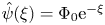 $\hat {\psi }(\xi )=\Phi _{0} {\rm e}^{-\xi }$ (Anderson et al. Reference Anderson, Lowell and Prieve1982; Sharifi-Mood et al. Reference Sharifi-Mood, Koplik and Maldarelli2013). The velocity monotonically grows away from the surface and approaches an asymptotic value, which upon multiplication with the tangential concentration gradient provides the Newtonian slip velocity. The viscoelastic component of the velocity field (
 $\hat {u}^{(0)}_{1}$), shown in figure 2(b), also grows monotonically away from the surface and attains an asymptotic value. The magnitude of this asymptotic value increases with the magnitude of interaction (
 $\Phi _{0}$).
The interactions between solute molecules and the particle surface can be either attractive or repulsive; if the solute is more attracted to the surface than the solvent, the interaction coefficient ( $\Phi _{0}$) is negative and viceversa. To show that the current analysis is valid for other forms of potential, we evaluate the velocity field inside the interaction layer for (i) an exponentially repulsive and (ii) a long-range van der Waals type interaction (arising primarily from the dipolar forces
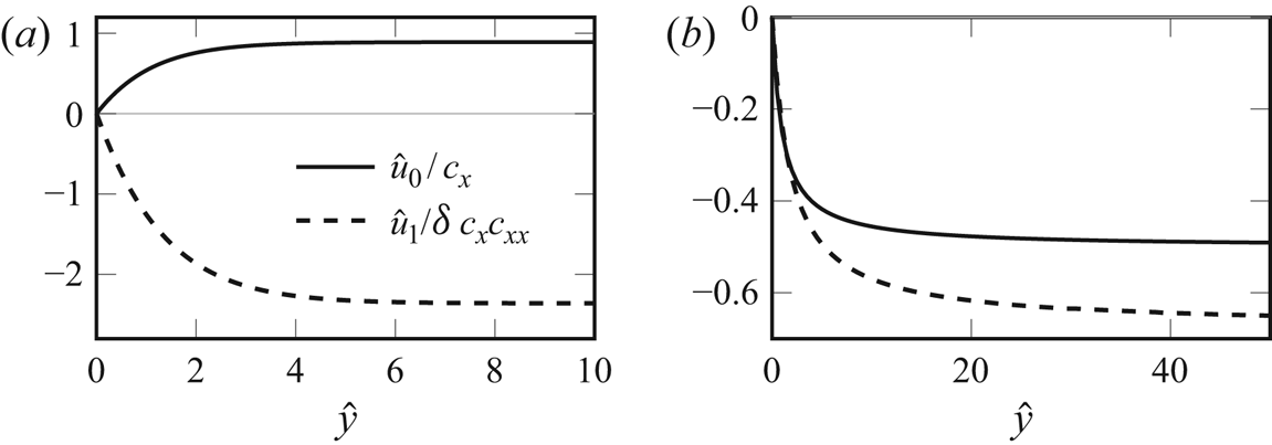
 ${\sim }1/r^{6}$). (i) For repulsive interactions, the thin ‘layer’ is characterized by an absence of solute concentration and the direction of motion (and slip) is opposite to that observed for an attractive interaction (Michelin & Lauga Reference Michelin and Lauga2014). Figure 3(a) shows that while the Newtonian slip is reversed (cf. figure 2a), the contribution from viscoelasticity is in the same direction as the case of attraction potential (cf. figure 2b). (ii) To incorporate long-range Lennard-Jones-type potential (attractive van der Waals interactions), we follow Anderson et al. (Reference Anderson, Lowell and Prieve1982, p. 112) and assume the dipolar interactions between the solute molecules to be pairwise additive. The potential is defined as
 \begin{equation} \hat{\psi}(\xi)=\Phi_{0} \left(- \frac{1}{(1+\xi)^{9}} + \frac{1}{(1+\xi)^{3}} \right). \end{equation}
The velocity fields (Newtonian and viscoelastic) remain qualitatively similar to that obtained from the attractive exponential interactions. As (2.22) decays slower than the exponential interaction, the asymptotic value (i.e. slip velocity) is obtained at larger distances from the surface.
Velocity field inside the interaction layer for (a) repulsive exponential interactions ( $\Phi _{0}=+1$) and (b) attractive long-range van der Waals interactions (
 $\Phi _{0}=-1$). Here,
 $c_{x}$ and
 $c_{xx}$ are the concentration gradients at the outer edge of the inner region i.e.
 $c_{x}\vert _{y=0}$ and
 $c_{xx}\vert _{y=0}$.

The above results demonstrate that the velocity fields inside the inner region approach an asymptotic value, the slip velocity. The Newtonian component of this slip is equal to the product of concentration gradient ( $c_{x}\vert _{y=0}$) and mobility coefficient
 $M_{0}$. Similarly, the viscoelastic component of velocity field involves
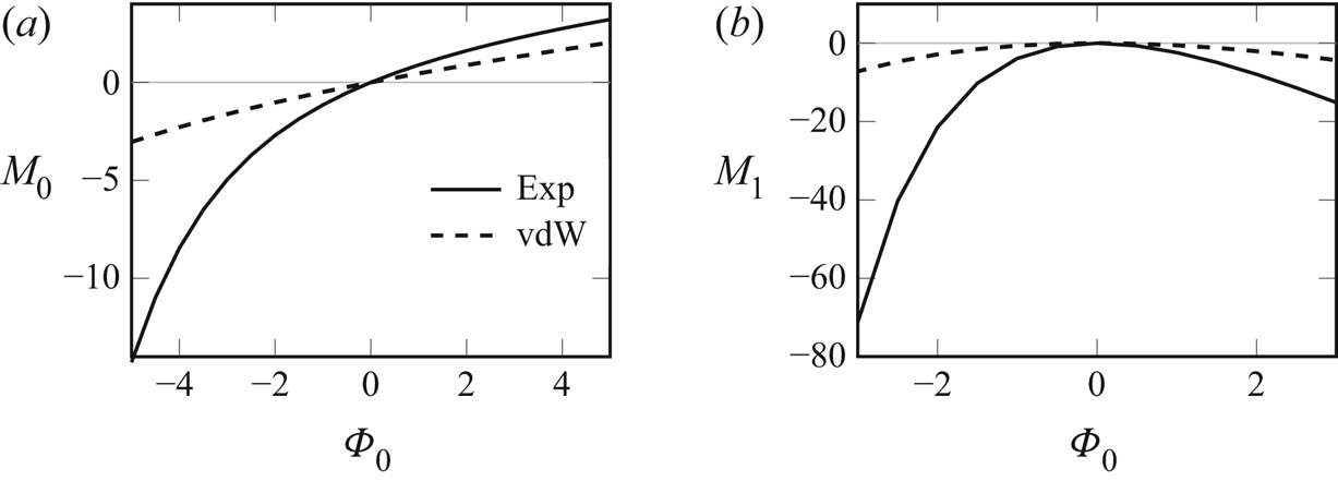
 $M_{1}$ (see (2.19)). The magnitude of mobility coefficients depends on the nature of interaction (exponential or van der Waals) and magnitude of attraction or repulsion (
 $\Phi _{0}$). Figure 4 quantifies the effect of the type and magnitude of interaction on
 $M_{0}$ and
 $M_{1}$. Figure 4(a) shows that the sign of Newtonian mobility coefficient is opposite for repulsive interactions (
 $\Phi _{0} > 0$) as compared to attractive ones (
 $\Phi _{0} < 0$), for both the type of interactions, i.e. short-range exponential or long-range van der Waals solute-surface interaction. Figure 4(b) shows that the sign of
 $M_{1}$ is always negative for both types of interactions. Furthermore, for repulsive interactions, the magnitude of mobility coefficients (
 $M_{0}$ and
 $M_{1}$) is reduced because the adsorption coefficient (characterizing the amount of solute excess near surface) in such cases is generally lower than that of attractive interactions (Anderson Reference Anderson1989, p. 69). For similar reasons, the exponential potential has higher mobility coefficient than that arising from van der Waals type interactions (Anderson et al. Reference Anderson, Lowell and Prieve1982, p. 113).
Variation of mobility coefficient (a)  $M_{0}$ and (b)
 $M_{1}$ with respect to
 $\Phi _{0}$, for exponential and van der Waals (vdW) interactions.

The above results, valid for moderate advective effects ( $\epsilon Pe \ll 1$), are also applicable to diffusio-osmotic flows of complex fluids in microchannels, arising from externally imposed concentration gradients or generated due to active ‘patches’ (Michelin et al. Reference Michelin, Montenegro-Johnson, De Canio, Lobato-Dauzier and Lauga2015; Michelin & Lauga Reference Michelin and Lauga2019).
Several experimental studies (Ke et al. Reference Ke, Ye, Carroll and Showalter2010; Ebbens & Howse Reference Ebbens and Howse2011; Baraban et al. Reference Baraban, Tasinkevych, Popescu, Sanchez, Dietrich and Schmidt2012) have shown that the particles are propelled with catalytic surface oriented at the rear-end, suggesting an attractive interaction between the solute molecules and active particle. Thus, we focus primarily on the exponentially attractive interaction because of its simplicity and ease of computation. We follow Sabass & Seifert (Reference Sabass and Seifert2012) and Sharifi-Mood et al. (Reference Sharifi-Mood, Koplik and Maldarelli2013) and assume  $| \Phi _{0} |=1$ in the results which follow.
2.2. Diffusio-osmotic slip on an active particle
We now extend the results of the previous section (2.19) to an axisymmetric Janus particle. Here, the direction normal to the surface is  $r$ and the tangential direction is polar angle
 $\theta$, varying from
 $0$ to
 ${\rm \pi}$. The surface activity
 $\mathcal {K}$ follows a step function (Golestanian et al. Reference Golestanian, Liverpool and Ajdari2007; Michelin & Lauga Reference Michelin and Lauga2014; Natale et al. Reference Natale, Datt, Hatzikiriakos and Elfring2017)
 \begin{equation} \mathcal{K} (\theta)= \begin{cases} 1, & \theta < \theta_{c},\\ 0, & \theta > \theta_{c}, \end{cases} \end{equation}
where  $\theta _{c}$ is the angle at which the activity undergoes a step change; it represents the surface coverage of activity. To evaluate the slip velocity, we require the solution to the concentration field (
 $c$) in the outer region. In the absence of advection (
 $Pe\rightarrow 0$), the solution to (2.8b) is sought in terms of an expansion in Legendre polynomials. Following Golestanian et al. (Reference Golestanian, Liverpool and Ajdari2007), we obtain the solution to bulk-scale concentration field as
 \begin{equation} c(r,\theta)=\displaystyle\sum_{n=0}^{\infty} {\frac{-\mathcal{K}_{n}}{(n+1)}}\, \frac{P_{n}(\cos \theta)}{r^{n+1}}, \end{equation}
where  $P_{n}$ is the
 $n$th-order Legendre polynomial. Here,
 $\mathcal {K}_{n}$ are the spectral coefficients of the activity distribution
 \begin{equation} \mathcal{K}(\theta)=\sum_{n=0}^{\infty} \mathcal{K}_{n} P_{n}(\cos\theta) . \end{equation}
These coefficients are found by taking an inner product of (2.25) with the Legendre polynomials (Michelin & Lauga Reference Michelin and Lauga2014), and are obtained as
 \begin{equation}\mathcal{K}_{0}=\frac{(1-\cos \theta_{c})}{2} \quad \text{and}\quad \mathcal{K}_{n}=\frac{-1}{2} (P_{n+1}(\cos \theta_{c}) - P_{n-1}(\cos \theta_{c})) \quad \text{for } n \geq 1. \end{equation}
Using the expression (2.24) for disturbance concentration, we obtain the total tangential slip velocity ( $M_{0} c_{\theta }(1,\theta ) + De \delta M_{1} c_{\theta }(1,\theta ) c_{\theta \theta }(1,\theta )$)
 \begin{align} \left.\boldsymbol{u}\right\vert_{r=1} = M_{0} \sum_{n=1}^{\infty} \frac{-\mathcal{K}_{n}}{n+1} \frac{\partial P_{n}}{\partial \theta} \boldsymbol{e}_{\theta} + De \, \delta M_{1} \left(\sum_{n=1}^{\infty} \frac{-\mathcal{K}_{n}}{(n+1)} \frac{\partial P_{n}}{\partial \theta} \right) \left(\sum_{n=1}^{\infty} \frac{-\mathcal{K}_{n}}{(n+1)} \frac{\partial^{2} P_{n}}{\partial \theta^{2}}\right) \boldsymbol{e}_{\theta}. \end{align}
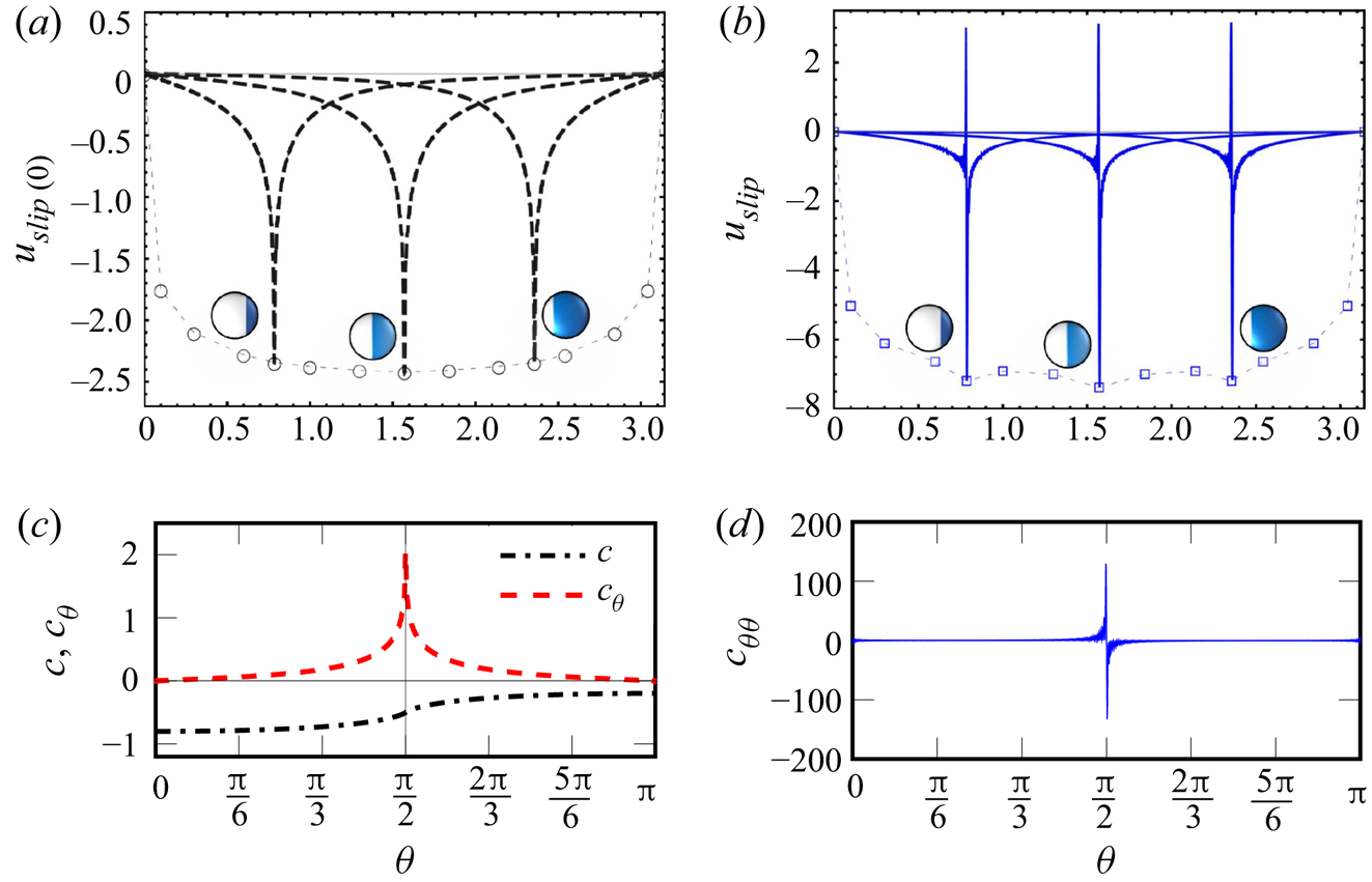
Figure 5(a) shows the Newtonian slip velocity varying across the polar angle for three different surface coverages ( $\theta _{c}={\rm \pi} /4, \, {\rm \pi} /2, \, 3{\rm \pi} /4$). The negative value shows that the diffusio-osmotic flow is towards the active region, and is highest in magnitude at the point of discontinuity of activity (
 $\theta =\theta _{c}$). (These results are validated with those reported by Michelin & Lauga (Reference Michelin and Lauga2014) and are provided in the supplementary material.) For a second-order fluid, figure 5(b) shows a localized reversal of slip velocity across
 $\theta _{c}$ for all three surface coverages, i.e. the slip velocity exhibits sharp nonlinear gradients across the point of discontinuity of activity. Natale et al. (Reference Natale, Datt, Hatzikiriakos and Elfring2017) also reported such behaviour in viscoelastic stresses at
 $\theta _{c}$ in their FEM simulations. They reported a viscoelasticity triggered extensional flow, across the point of discontinuity in surface activity.
(a) The dashed line represents the Newtonian slip velocity along the polar angle for three different surface coverages ( $\theta _{c}={\rm \pi} /4, {\rm \pi} /2, 3{\rm \pi} /4$). The empty circular markers represent the maximum magnitude of the slip velocity for a range of surface coverage:
 $\theta _{c} \in (0,{\rm \pi} )$. (b) The solid line represents the total slip velocity (for three different surface coverages) along the polar angle for
 $\hat {\psi }(\xi )=- {\rm e}^{-\xi }$,
 $De=0.01$ and
 $\delta =-0.5$ (corresponds to
 $\Psi _{2}^{*}=0$). The empty square markers represent the maximum magnitude of the slip velocity for a range of surface coverage:
 $\theta _{c} \in (0,{\rm \pi} )$. (c) Concentration profile and its gradient along the polar angle (on particle surface) for
 $\theta _{c}={\rm \pi} /2$. Panel (d) shows the profile for
 $c_{\theta \theta }$. First 700 modes were used to describe the concentration field and its gradients.

To analyse this slip reversal or the extensional flow across the point of transition in activity, we examine the behaviour of the concentration field around the particle, as the slip (2.19) depends on the first and second polar gradient of the concentration field. In figure 5(c,d),  $c$,
 $c_{\theta }$ and
 $c_{\theta \theta }$ profiles are shown for
 $\theta _{c}={\rm \pi} /2$. A step change in surface activity causes the second tangential gradient to undergo a sharp reversal at
 $\theta =\theta _{c}$, which is also reflected in the slip velocity (in figure 5b). The profile of
 $c_{\theta \theta }$, despite accounting for first 700 modes, exhibits oscillations near the point of discontinuity of surface activity. This seemingly divergent behaviour is because of the step function representation of surface activity (2.23), which is widely employed in the literature (Golestanian et al. Reference Golestanian, Liverpool and Ajdari2007; Michelin & Lauga Reference Michelin and Lauga2014; Natale et al. Reference Natale, Datt, Hatzikiriakos and Elfring2017). This oscillatory behaviour indicates a violation of scaling in the inner region: in § 2.1.2 the length scale in the tangential direction was assumed to be
 $a^{*}$, which is not the true characteristic of the system as variations in the tangential direction are rapid for a step discontinuity in surface activity. Since such step discontinuities are unlikely to be realized in experiments, we now consider a smooth variation in the activity and demonstrate that the oscillatory behaviour of
 $c_{\theta \theta }$ for step activity is a mathematical artefact.
2.3. Diffusio-osmotic slip on an active particle: sigmoidal function approximation
The step change in surface activity is approximated as a logistic function
 \begin{equation} \mathcal{K}(\theta)={1}/\!\left( {1+ \exp\left[{-\zeta \left(\theta_{c}- \theta \right)}\right]}\right). \end{equation}
Here,  $\zeta$ (transition parameter) determines the sharpness of the transition ofnon-dimensional activity from 1 to 0. We have chosen
 $\zeta =16$ such that the transition length is large enough to maintain the consistency of the analysis with respect to the scaling used in § 2.1.2 (i.e.
 $l_{transition}^{*} \sim a^{*}$). (For a particle of
 $a^{*}=5\ {\rm \mu} \textrm {m}$,
 $\zeta =16$ corresponds to a circumferential length of
 ${\sim } 2 \ {\rm \mu} \textrm {m}$, which is much larger than the typical interaction layer thickness.) The expressions for concentration and slip velocity are identical to (2.24) and (2.27), respectively. The spectral modes can be found by substituting (2.28) into (2.25) and taking the inner product with respect to
 $P_{n}$ on both sides
 \begin{equation} \mathcal{K}_{n}=\frac{2n+1}{2} \int_{0}^{{\rm \pi}} \mathcal{K}(\theta) P_{n}(\cos \theta)\, {\textrm{d}}\theta. \end{equation}
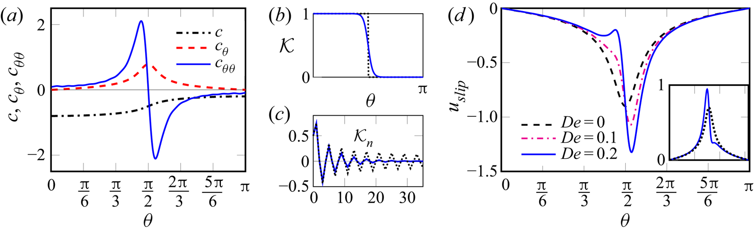
For activity represented by (2.28), the concentration field and its tangential gradients (at the surface) are depicted in figure 6(a). The variation of concentration field and its gradients along  $\theta$ is qualitatively similar to that reported for the step change; the magnitudes, however, are significantly reduced. Figures 6(b) and 6(c) show the variation of activity and its faster convergence in comparison to the step function. Figure 6(d) compares the slip velocity for a second-order fluid with that of a Newtonian fluid.
(a) Profile of concentration and its first and second gradient along the polar angle on particle surface for  $\theta _{c}={\rm \pi} /2$. (b) Variation of surface activity as a step (dotted line) and smooth function (solid line). (c) Convergence of spectral modes: solid (blue) line shows fast convergence for the sigmoidal activity; and dotted (black) line depicts slow convergence for step activity. (d) Different curves represent the total slip velocity along the polar angle for
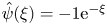 $\hat {\psi }(\xi )=-1 {\rm e}^{-\xi }$,
 $\zeta =16$,
 $\delta =-0.5$ and different Deborah numbers. The inset shows the slip velocities for Newtonian and second-order fluid for the case of repulsive interactions:
 $\Phi _{0}=+1$,
 $De = 0$ (
 , black) and
 $De = 0.2$ (
 , blue).

We observe a reduction and an increase in slip velocity (relative to the Newtonian slip) across  $\theta _{c}$. The magnitude of modification in the slip is significantly reduced (as compared with that of step change in activity) which is a consequence of smooth transition of activity. The above observations are for attractive interactions between solute and particle surface; for repulsive interactions (as shown in the inset of figure 6d), the effect of viscoelasticity is qualitatively reversed.
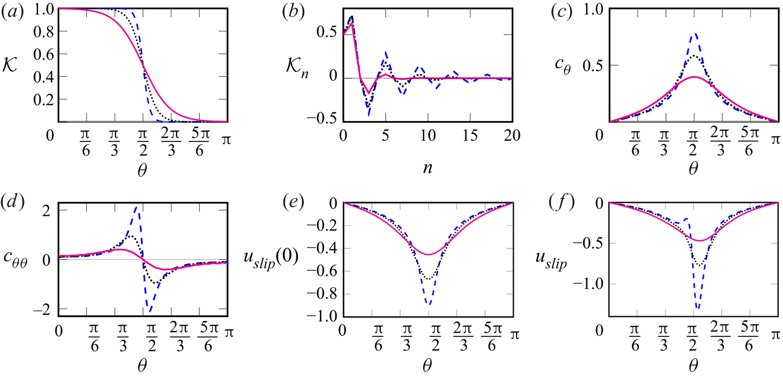
Figure 7 demonstrates the effect of the transition parameter ( $\zeta$) on the convergence of spectral coefficients, concentration gradients and slip velocity. Figure 7(a) shows that as
 $\zeta$ decreases, the transition from active to passive surface becomes smoother. Figure 7(b) shows that the convergence is faster for lower
 $\zeta$. As the transition becomes smoother the magnitude of tangential gradients of concentration field reduces (figure 7c,d). As a result, the slip velocity for Newtonian and second-order fluid reduces (shown in figure 7(e–f), respectively).
Analysis of activity, spectral modes, concentration gradients and slip velocity for three different transition parameters:  $\zeta =4$ (
 , pink),
 $\zeta =8$ (, black), and
 $\zeta =16$ (
 , blue). (a) Variation of activity with polar angle
 $\theta$. (b) Convergence of spectral modes. (c) Tangential concentration gradient. (d) Second tangential derivative of concentration field. (e) Slip velocity of a Newtonian fluid. (f) Slip velocity of the second-order fluid. Parameters:
 $De=0.2$,
 $\delta =-0.5$,
 $\Phi _{0}=-1$.

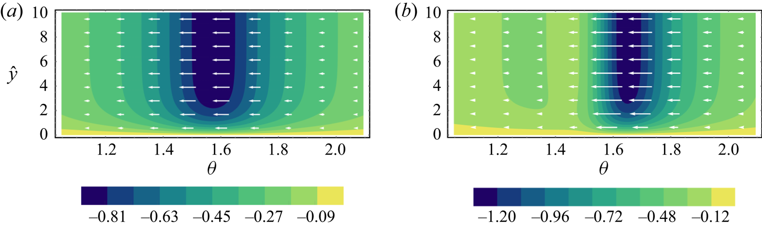
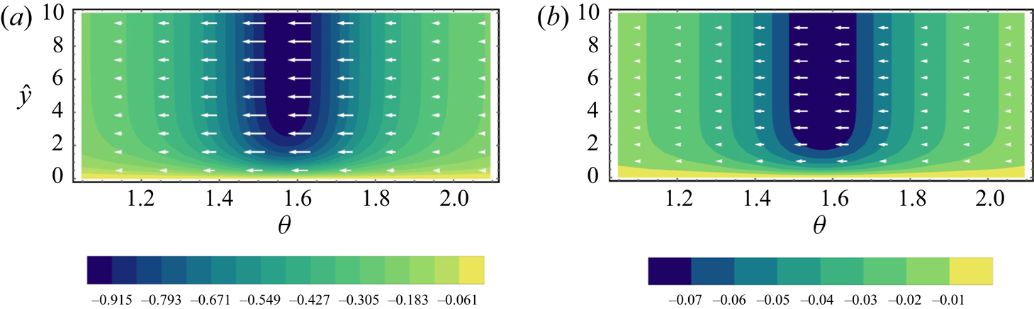
The effect of viscoelasticity on the tangential velocity field inside the interaction layer is shown in figure 8 (for  $\theta _{c}={\rm \pi} /2$). Figure 8(a) depicts the symmetry of velocity field across
 $\theta _{c}$ for Newtonian fluid. Addition of viscoelasticity breaks this symmetry: the contours of the SOF in figure 8(b) depict that the magnitude of velocity field is reduced before the transition of activity (
 $\theta < \theta _{c}$) and increased after it (
 $\theta > \theta _{c}$). These results suggest that the elastic effects (characterized by
 $De$) tend to locally reverse the slip velocity. At higher Deborah numbers, a reversal in slip velocity can generate a local extensional flow near the transition of activity (as shown by Natale et al. (Reference Natale, Datt, Hatzikiriakos and Elfring2017)), resembling a puller or pusher-type flow field. Interestingly, there have been similar observations in the context of electrophoresis. Recently, Li & Koch (Reference Li and Koch2020) reported that, in weakly viscoelastic fluids, polymer elasticity in the inner region changes the electrophoretic particle into a puller-type squirmer: the strong shear flow in the double layer causes the polymers to be stretched tangentially, resulting in a pulling flow at the front and rear end, and a pushing flow from the sides. Since electrophoretic and diffusiophoretic mechanisms share qualitative similarities (such as strong shear inside the thin layer), it is plausible that the effects of elasticity, observed in electrophoresis, emerge in diffusiophoresis as well.
(a) Newtonian tangential velocity contours inside the interaction layer for  $\theta _{c}={\rm \pi} /2$. (b) Tangential velocity contours corresponding to the second-order fluid for
 $\hat {\psi }(\xi )=- {\rm e}^{-\xi }$,
 $\zeta =16$,
 $\delta =-0.5$ and
 $De=0.2$. Arrows depict the velocity vectors (
 $\hat {\boldsymbol {u}}_{1}^{(0)}$).

2.4. Swimming velocity
The motion of the Janus sphere is found by using the reciprocal theorem. Following Stone & Samuel (Reference Stone and Samuel1996) and Ho & Leal (Reference Ho and Leal1976), we obtain the swimming velocity as
 \begin{equation} U=\frac{-1}{4{\rm \pi}} \int_{S_{p}} \left.\left( \boldsymbol{u}_{0} + De \,\boldsymbol{u}_{1} \right)\right\vert_{r=1} \boldsymbol{\cdot} \boldsymbol{e}_{z} \, \textrm{d}S - \frac{1}{6{\rm \pi}} De \int_{V_{f}} \boldsymbol{\mathsf{S}}_{\,0}\boldsymbol{:} \boldsymbol{\nabla}{\boldsymbol{u}^{t}}\, \textrm{d}V. \end{equation}
Here,  $\boldsymbol {u}_{0}$ is the Newtonian slip velocity (
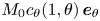 $M_{0} c_{\theta }(1,\theta ) \, \boldsymbol {e}_{\theta }$),
 $De \, \boldsymbol {u}_{1}$ is the modification to slip due to viscoelasticity (
 $De \, M_{1} \delta \, c_{\theta }(1,\theta ) \, c_{\theta \theta }(1,\theta ) \, \boldsymbol {e}_{\theta }$),
 $\boldsymbol {u}^{t}$ is the test flow field which governs the motion of a rigid sphere in
 $z$-direction with unit velocity in a quiescent Newtonian medium (Michelin & Lauga Reference Michelin and Lauga2014; Datt et al. Reference Datt, Zhu, Elfring and Pak2015) and
 $\boldsymbol{\mathsf{S}}_{\,0}$ is the polymeric stress. The first integral (
 $U_{\lambda }$) denotes the contribution to swimming velocity arising from the slip, which contains a Newtonian (
 $U_{\lambda _0}$) and a non-Newtonian (
 $U_{\lambda _1}$) component
 \begin{align} U_{\lambda_{0}} = \frac{M_{0}}{2} \int_{0}^{{\rm \pi}} c_{\theta}(1,\theta) \sin^{2}{\theta} \, {\textrm{d}}\theta; \quad U_{\lambda_{1}} = \frac{De\, \delta M_{1}}{2} \int_{0}^{{\rm \pi}} c_{\theta}(1,\theta) c_{\theta \theta}(1,\theta) \sin^{2}{\theta} \, {\textrm{d}}\theta. \end{align}
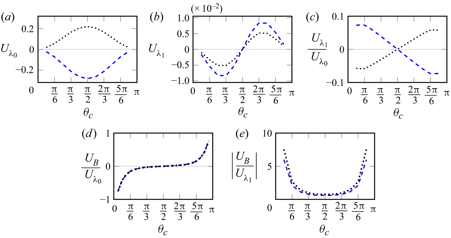
We evaluate the above components and compare them in figure 9 for different surface coverages. For attractive interactions between the solute molecules and particle, the Newtonian swimming velocity is in the negative  $z$-direction (see figure 9a). Figures9(b) and 9(c) show that the modification to the swimming velocity (
 $U_{\lambda_{1}}$ contribution) is relatively small and changes sign with the surface coverage: the swimming velocity increases for
 $\theta _{c}<{\rm \pi} /2$ and reduces for
 $\theta _{c}>{\rm \pi} /2$.
(a) Variation of swimming velocity due to Newtonian surface slip ( $U_{\lambda _{0}}$) for various surface coverages. (b) Perturbation to swimming velocity due to modification in the slip (
 $U_{\lambda _{1}}$). (c) Ratio of the swimming velocity components, i.e. (b) and (a). (d) Variation of modification to the swimming velocity due to bulk polymeric stresses (
 $U_{B}$). (e) Ratio of (d) and (c): comparison of two components arising due to viscoelasticity. Parameters:
 $De=0.1$,
 $\delta =-0.5$,
 $\zeta =16$,
 $\Phi _{0}=-1$ (attractive; , blue) and
 $\Phi _{0}=+1$ (repulsive; , black).

For a repulsive interaction,  $U_{\lambda _{0}}$ changes sign (depicting swimming in the opposite direction) as also reported by earlier studies (Sharifi-Mood et al. Reference Sharifi-Mood, Koplik and Maldarelli2013; Michelin &Lauga Reference Michelin and Lauga2014; Natale et al. Reference Natale, Datt, Hatzikiriakos and Elfring2017). The contribution of
 $U_{\lambda _{1}}$ is such that the swimming velocity is reduced for
 $\theta _{c} < {\rm \pi} /2$ and enhanced for
 $\theta _{c} > {\rm \pi} /2$. Here,
 $U_{\lambda _{1}}$ is in the same direction as that for attractive interaction. This outcome can be understood by comparing the flow field inside the interaction layer for attractive and repulsive cases, i.e. figures 2 and 3(a), respectively. In comparison to the attractive interaction, Newtonian velocity field was reversed for repulsive interactions, whereas the modification (arising from viscoelasticity) was found to be in the same direction. It is also interesting to note that, contrary to
 $U_{\lambda _{0}}$,
 $U_{\lambda _{1}}$ is an odd function (antisymmetric about
 ${\rm \pi} /2$) which is due to the proportionality to double tangential derivative of surface concentration, whereas the former is solely proportional to the single tangential derivative.
The second integral ( $U_{B}$) accounts for the contribution from polymeric stresses in the bulk. In their evaluation of swimming velocity, Datt et al. (Reference Datt, Natale, Hatzikiriakos and Elfring2017) accounted for the bulk viscoelastic effects (
 $U_{B}$), and provided the following analytical expression (re-expressed here using the scales in (2.5a–d)):
 \begin{equation} \frac{U_{B}}{U_{\lambda_{0}}} = - De (1+\delta) \sum_{n=1}^{\infty} \frac{6n}{(n+1)^{2} (n+2)} \frac{\alpha_{n} \alpha_{n+1}}{\alpha_{1}^{2}}, \end{equation}
where  $\alpha _{n} = {n \mathcal {K}_{n}}/{(2n+1)}$ and
 $\mathcal {K}_{n}$ is determined using (2.28) and (2.29). The modification due to the bulk stresses (
 $U_{B}/U_{\lambda _{0}}$) is plotted in figure 9(d) for smooth activity. The figure shows that
 $U_{B}$ can significantly enhance (or impede) the active swimming, depending upon the surface coverage (
 $\theta _{c}$) being more (or less) than
 ${\rm \pi} /2$. This was also reported by Datt et al. (Reference Datt, Natale, Hatzikiriakos and Elfring2017) for step activity. A comparison of the two effects of viscoelasticity,
 $U_{B}$ and
 $U_{\lambda _{1}}$ (shown in figure 9e), reveals that the contribution to the swimming velocity from the modification in slip (
 $U_{\lambda _{1}}$) is comparable to that from
 $U_{B}$ for
 $5{\rm \pi} /6 < \theta _{c}<{\rm \pi} /6$.
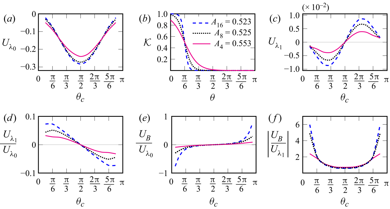
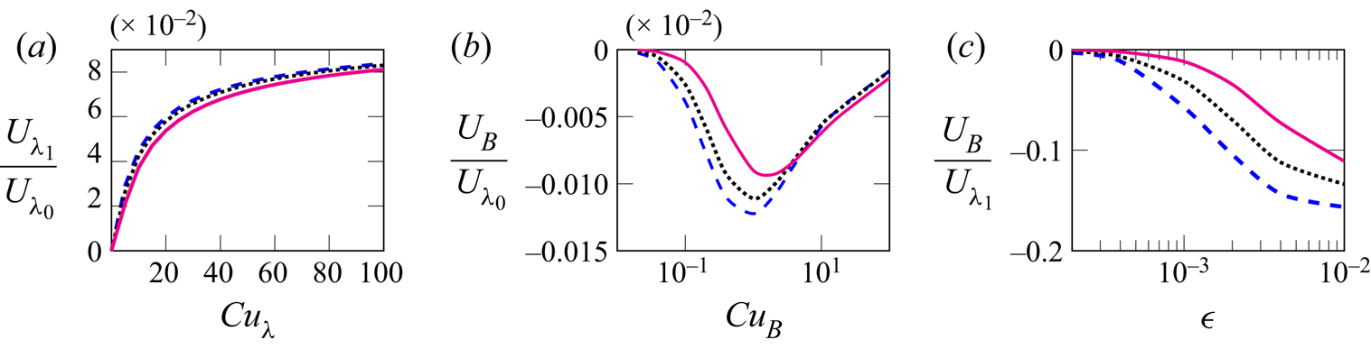
Figure 10 shows the effect of transition parameter ( $\zeta$) on the components of swimming velocity for various surface coverages. As
 $\zeta$ decreases the Newtonian swimming velocity reduces (figure 10a) because the slip velocity decreases (shown in figure 7). However, for
 $\theta _{c}<{\rm \pi} /4 \,\hbox{and}\, \theta _{c}>3{\rm \pi} /4$,
 $U_{\lambda _{0}}$ is greatest for
 $\zeta =4$. This is because, for such coverages, the total area of catalytic activity is more for
 $\zeta =4$ than the steeper activity transitions (
 $\zeta =8,16$). Figure 10(b) shows the area under the
 $\mathcal {K}-\theta$ curve for
 $\zeta =4,8,16$, representing the total area of activity for
 $\theta _{c}={\rm \pi} /6$. For
 ${\rm \pi} /4 < \theta _{c} < 3{\rm \pi} /4$, the area of catalytic activity is independent of
 $\zeta$ and thus a direct comparison can be made. Figures 10(c) and 10(d) show that the contribution from
 $U_{\lambda _{1}}$ reduces as
 $\zeta$ decreases, which is due to significant reduction in slip velocity. Similarly, the contribution from bulk polymeric stresses reduces as
 $\zeta$ decreases, as shown in figure 10(e,f).
Analysis of different components of swimming velocity for three different transition parameters:  $\zeta =4$ (, pink),
 $\zeta =8$ (, black), and
 $\zeta =16$ (, blue). (a) Variation of
 $U_{\lambda _{0}}$ with different surface coverages. (b) Variation of activity
 $\mathcal {K}$ with polar angle
 $\theta$. (c) Variation of
 $U_{\lambda _{1}}$ for different surface coverages. (d) Contribution from the slip modification to the swimming velocity for different surface coverages. (e) Bulk stress contribution to the swimming velocity for different surface coverages. (f) Comparison of (e) with (d) (i.e.
 $U_{B}$ with
 $U_{\lambda _{1}}\!$) for different surface coverages. Parameters:
 $De=0.1$,
 $\delta =-0.5$,
 $\Phi _{0}=-1$.

3. Active particle in a shear-thinning fluid
The equations governing a weak shear-thinning flow are described by
 \begin{equation} \boldsymbol{\nabla}^{*} \boldsymbol{\cdot} \boldsymbol{u}^{*}=0, \quad -\boldsymbol{\nabla}^{*} p^{*} + \boldsymbol{\nabla}^{*} \boldsymbol{\cdot} \left( \mu^{*} \boldsymbol{\mathsf{A}}^{*} \right) -C^{*} \boldsymbol{\nabla}^{*} \mathcal{P}^{*} =\boldsymbol{0}. \end{equation}
The viscosity follows a general nonlinear relation with respect to Newtonian shear-rate ( $\gamma _{0}$) (Khair et al. Reference Khair, Posluszny and Walker2012),
 $\mu ^{*}(\gamma _{0})=\mu ^{*}_{0} ({1+\chi \mu _{1}(\gamma _{0})})$. Here,
 $\chi$ is a small parameter which represents the viscosity ratio,
 $(\mu _{0}^{*} - \mu _{\infty }^{*})/{\mu _{\infty }^{*}}$, the zero shear rate viscosity is
 $\mu _{0}^{*}$, and
 $\mu _{\infty }^{*}$ is the infinite shear rate viscosity. The variables are non-dimensionalized as in § 2. Since the concentration field is decoupled from the hydrodynamics (provided
 $\epsilon ^{2} Pe \ll 1$), the solution to concentration field is unchanged and is given by (2.14a).
3.1. Evaluation of the diffusio-osmotic slip
Similar to § 2.1, we use matched asymptotic expansion (assuming  $Pe \ll \epsilon ^{-2}$ and
 $\epsilon \ll 1$) and perturbation expansion (in
 $\epsilon$) to obtain the leading-order slip for a generalized weakly shear-thinning fluid.
3.1.1. Outer region
At the leading order, the equations in the outer region are
 \begin{equation} \boldsymbol{\nabla} \boldsymbol{\cdot} \boldsymbol{u}^{(0)} = 0, \quad - \boldsymbol{\nabla} p^{(0)} + {\mu(\gamma_{0})} {\nabla}^{2} \boldsymbol{u}^{(0)} + \boldsymbol{\nabla} {\mu(\gamma_{0})} \boldsymbol{\cdot} \boldsymbol{\mathsf{A}}^{(0)} = \boldsymbol{0}, \end{equation}
subject to the following boundary conditions:
 \begin{equation} \boldsymbol{u}^{(0)} \rightarrow \boldsymbol{0} , \; p^{(0)} \rightarrow 0 \quad \text{as } y \rightarrow \infty. \end{equation}
Here,  $\mu (\gamma _{0}) = \mu ^{*} / \mu ^{*}_{0} = 1+\chi \mu _{1}(\gamma _{0})$.
3.1.2. Inner region
We rescale the variables (similar to § 2.1.2) and obtain the governing equations in the inner region (at the leading order) as
 \begin{gather} \frac{\partial \hat{u}^{(0)}}{\partial \hat{x}} + \frac{\partial \hat{v}^{(0)}}{\partial \hat{y}} =0 , \end{gather}
 \begin{gather} - \frac{\partial \hat{p}^{(0)}}{\partial \hat{x}} + {\mu(\gamma_{0})} \frac{\partial^2 \hat{u}^{(0)}}{\partial \hat{y}^2} + \frac{\partial \mu(\gamma_{0})}{\partial \hat{y}} \frac{\partial \hat{u}^{(0)}}{\partial \hat{y}} = (\hat{c}^{(0)} + C_{\infty})\frac{\partial \hat{\psi}^{(0)}}{\partial \hat{x}} , \end{gather}
 \begin{gather} - \frac{\partial \hat{p}^{(0)}}{\partial \hat{y}} = (\hat{c}^{(0)}+C_{\infty}) \frac{\partial \hat{\psi}^{(0)}}{\partial \hat{y}} , \end{gather}
subject to the pressure decay and no-slip boundary condition
 \begin{equation} \hat{p} \rightarrow 0 \ \textrm{{as}} \ \hat{y} \rightarrow \infty; \quad \left. \hat{u}^{(0)} \right\vert_{\hat{y}=0} = 0. \end{equation}
Assuming that the difference between zero shear and infinite shear viscosity is small (i.e.  $\chi \ll 1$), we perform a regular perturbation expansion in
 $\chi$ and represent the velocity and pressure fields as
 \begin{equation} f^{(i)}(x,y)=f^{(i)}_{0}(x,y)+\chi \, f^{(i)}_{1}(x,y)+\cdots . \end{equation}
Substituting the perturbed field variables in (3.4)–(3.5) gives the equations governing the system at  $O(1)$ and
 $O(\chi )$.
At  $O(1)$, the equations and their solutions are identical to (2.14). The hydrodynamics at
 $O(\chi )$ is governed by
 \begin{gather} \frac{\partial \hat{u}_{1}^{(0)}}{\partial \hat{x}} + \frac{\partial \hat{v}_{1}^{(0)}}{\partial \hat{y}} =0 , \end{gather}
 \begin{gather} - \frac{\partial \hat{p}_{1}^{(0)}}{\partial \hat{x}} + \frac{\partial^2 \hat{u}_{1}^{(0)}}{\partial \hat{y}^2} + \mu_{1}(\gamma_{0}) \frac{\partial^2 \hat{u}_{0}^{(0)}}{\partial \hat{y}^2} + \frac{\partial \mu_{1}(\gamma_{0})}{\partial \hat{y}} \frac{\partial \hat{u}_{0}^{(0)}}{\partial \hat{y}} = 0 , \end{gather}
 \begin{gather} - \frac{\partial \hat{p}_{1}^{(0)}}{\partial \hat{y}} = 0. \end{gather}
Integrating (3.7c) and using the pressure decay condition, we get  $\hat {p}_{1}^{(0)} = 0$. (3.7b) thus yields
 \begin{equation} \frac{\partial^{2} \hat{u}_{1}^{(0)}}{\partial \hat{y}^{2}} = - \frac{\partial}{\partial \hat{y}} \left( \mu_{1}(\gamma_{0}) \frac{\partial \hat{u}_{0}^{(0)}}{\partial \hat{y}} \right). \end{equation}
Integrating the above equation twice gives
 \begin{align} \hat{u}_{1}^{(0)} = \mathcal{I}'(\hat{x}) \int_{0}^{\hat{y}} \mu_{1}(\gamma_{0}) \int_{t}^{\infty} \mathcal{F}(s)\,\textrm{d}s \, \textrm{d}t - \mathcal{J}_{0}(\hat{x}) \int_{0}^{\hat{y}} \mu_{1} (\gamma_{0})\,\textrm{d}s \; + \left(\mathcal{J}_{1}(\hat{x}) - \mathcal{J}_{0} (\hat{x}) \mu_{1}\right) \hat{y}, \end{align}
where  $\mathcal {F}(s) = -1 + {\rm e}^{-\hat {\psi }(s)}$.
3.1.3. Matching
As in § 2.1.3, upon matching the inner and outer solutions, we find that  $\mathcal {J}_{0}=\mathcal {J}_{1}=0$ and obtain
 \begin{equation} \left. u^{(0)} \right\vert_{y=0} = \left. c^{(0)}_{x}\right\vert_{y=0} \left( M_{0} + \chi \, M_{1} \right), \end{equation}
where  $M_{0}$ is the mobility coefficient representing the Newtonian contribution and is expressed in (2.20a,b). The expression for
 $M_{1}$ is
 \begin{equation} M_{1} = {\displaystyle\int_{0}^{\infty} } \mu_{1}\left(\gamma_{0}^{(0)}\right) \int_{t}^{\infty} \mathcal{F}(s)\,\textrm{d}s \, \textrm{d}t . \end{equation}
Since the power-law model diverges for asymptotically small shear-rates (Bird et al. Reference Bird, Armstrong and Hassager1987), we choose the Carreau model to capture viscosity variation:  $\mu _{1}=( 1+ \tau ^{*\,2} |\gamma _{0}^{*}|^{2} )^{({n-1})/{2}} - 1$ (Bird et al. Reference Bird, Armstrong and Hassager1987). Here,
 $\tau ^{*}$ is the fluid relaxation time scale and
 $n$ characterizes the degree of shear-thinning (
 $n<1$). For Carreau fluid, the non-Newtonian mobility coefficient (
 $M_{1}$)is
 \begin{equation} M_{1} = {\displaystyle\int_{0}^{\infty} } \left\{ \left[ 1 + \left( C\!u_{\lambda} \, \left. c_{x}^{(0)}\right\vert_{y=0} \int_{t}^{\infty} \mathcal{F}(s)\, {\textrm{d}}s \right)^{2} \right]^{({n-1})/{2}} -1 \right\} \int_{t}^{\infty} \mathcal{F}(s) \,\textrm{d}s \, \textrm{d}t , \end{equation}
where  $C\!u_{\lambda }$ (based on shear in the interaction layer) is the ratio of time scales associated with relaxation (
 $\tau ^{*}$) to that of shear in the flow (
 $\lambda _{I}^{*}/U_{ch}$),
 $C\!u_{\lambda } = \tau ^{*}/(\lambda _{I}^{*}/U_{ch})$. This is different than the Carreau number corresponding to shear in the bulk fluid (i.e. outer region):
 $C\!u_{B} = \tau ^{*}/(a^{*}/U_{ch})$. The ratio of the two Carreau numbers (
 $C\!u_{\lambda }/C\!u_{B} = a^{*}/\lambda _{I}^{*}$) provides the comparison of shear rate inside to that outside the interaction layer, i.e.
 $O(\epsilon ^{-1})$.
3.2. Diffusio-osmotic slip on an active particle
As in § 2.2, we now apply the above results to an axisymmetric Janus sphere. Since the shear in the thin interaction layer is generally high (i.e.  $U_{ch}/\lambda _{I}^{*} \sim 10^{2} \ \textrm {s}^{-1}$) and relaxation time scales of the biological fluids are
 ${\sim }1\,{\rm s}$ (Zare, Park & Rhee Reference Zare, Park and Rhee2019), large Carreau numbers are possible (
 $C\!u_{\lambda } \sim 10^{2}$). Contrary to the second-order fluid,
 $M_{1}$ for Carreau fluid depends both on the magnitude of interaction (
 $\Phi _{0}$) as well as the concentration gradient (determined by the activity transition parameter
 $\zeta$). Since the concentration field varies in the tangential direction,
 $M_{1}$ varies tangentially. Thus, we analyse the effect of
 $\Phi _{0}$ and
 $\zeta$ on
 $M_{1}$ for
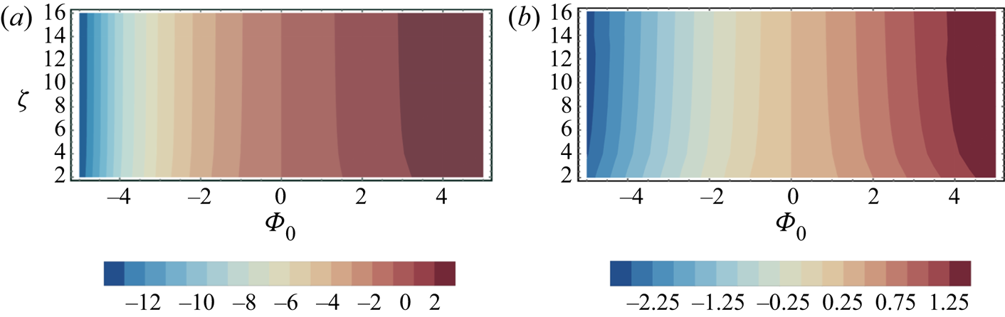
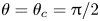 $\theta =\theta _{c}={\rm \pi} /2$ in figure 11. For both short-range exponential and long-range van der Waals interactions,
 $M_{1}$ is a weak function of
 $\zeta$. Here,
 $M_{1}$ for Carreau fluid is of a different sign for attractive (
 $\Phi _{0}<0$) and repulsive interactions (
 $\Phi _{0}>0$), as opposed to the case of second-order fluid (figure 4b).
Non-Newtonian mobility ( $M_{1}$) at
 $\theta ={\rm \pi} /2$ for two interaction potentials: (a) exponential type and (b) van der Waals type. Other parameters:
 $n=0.25$,
 $C\!u_{\lambda }=10^{2}$,
 $\theta _{c}={\rm \pi} /2$.

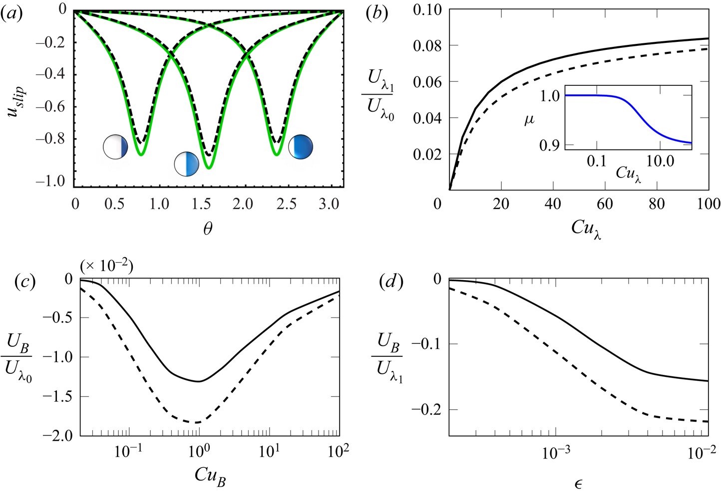
Using (2.24), (2.28), (3.10) and (3.12), we numerically evaluate the slip for shear-thinning fluid ( $n=0.25$) and depict its variation along the surface of Janus particle in figure 12(a). For large Carreau numbers (
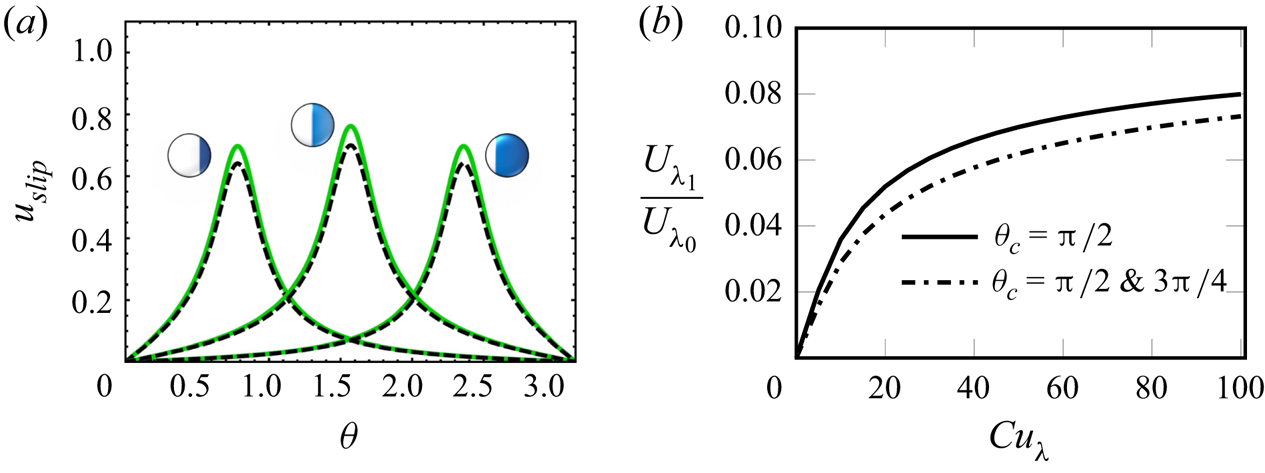
 $C\!u_{\lambda } \sim 10^{2}$) and attractive interactions, we find a marginal increase in the total slip velocity. For repulsive interactions, the enhancement in slip velocity is qualitatively similar (see the Appendix). The modification in slip (in both attractive and repulsive cases) is maximum at the transition of activity, depicting a local symmetry about
 $\theta _{c}$.
(a) The dashed black line represents the Newtonian slip velocity. The solid green line represents the variation of total slip velocity for a shear thinning fluid along the polar angle for  $\hat {\psi }(\xi )=- {\rm e}^{-\xi }$ and
 $C\!u_{\lambda }=100$. (b) Variation of non-Newtonian contribution to the swimming velocity (arising from the surface slip) with
 $C\!u_{\lambda }$, for three different surface coverage (
 $\theta _{c}$) and
 $\hat {\psi }(\xi ) = -{\rm e}^{-\xi }$. Solid (, black) and dashed lines (}, black) correspond to
 $\theta _{c}={\rm \pi} /2$ and
 $\theta _{c}={\rm \pi} /4$ or
 $3{\rm \pi} /4$, respectively. Inset showing the variation in non-dimensional viscosity
 $\mu$ with
 $C\!u_{\lambda }$ at
 $y=0$ and
 $\theta =\theta _{c}={\rm \pi} /2$. (c) Variation of non-Newtonian contribution to the swimming velocity (arising from the bulk stresses) with
 $C\!u_{B}$. The convergence was obtained by accounting for first 15 modes. (d) Comparison between the two non-Newtonian components of swimming velocity for
 $C\!u_{\lambda }=10^{2}$. Other parameters:
 $\chi =0.1$,
 $n=0.25$,
 $\zeta =16$.

3.3. Swimming velocity
We now evaluate the swimming velocity using the reciprocal theorem (Stone & Samuel Reference Stone and Samuel1996; Khair et al. Reference Khair, Posluszny and Walker2012)
 \begin{equation} U=\frac{-1}{4{\rm \pi}} \int_{S_{p}} \left.\left( \boldsymbol{u}_{0} + \chi \,\boldsymbol{u}_{1} \right)\right\vert_{r=1} \boldsymbol{\cdot} \boldsymbol{e}_{z} \, \textrm{d}S \; - \; \frac{1}{6{\rm \pi}} \chi \int_{V_{f}} \mu_{1} \left( \gamma_{0} \right) \boldsymbol{\mathsf{A}}_{0} \boldsymbol{:} \boldsymbol{\nabla}{\boldsymbol{u}^{t}}\,\textrm{d}V. \end{equation}
As in § 2.4, the first integral contains the Newtonian component  $U_{\lambda _0}$ (given by (2.31a,b)) and non-Newtonian component
 $U_{\lambda _1}$
 \begin{equation} U_{\lambda_{1}} = \frac{\chi}{2} \int_{0}^{{\rm \pi}} M_{1}(\theta) c_{\theta}(1,\theta) \sin^{2} \theta\, \textrm{d}\theta. \end{equation}
Substituting (3.12) in (3.13) and integrating numerically, we find that the contribution from  $U_{\lambda _1}$ modestly affects the swimming of a Janus particle. This is shown in figure 12(b) for three different surface coverages. The positive sign of the ratio shows that
 $U_{\lambda _1}$ adds to the contribution arising from the Newtonian slip (
 $U_{\lambda _{0}}$). As
 $C\!u_{\lambda }$ increases, the viscosity in the interaction layer decreases, which results in a faster diffusio-osmotic flow. However, this enhancement reaches a plateau as the viscosity reduction stagnates at high
 $C\!u_{\lambda }$ (see inset in figure 12b). For repulsive interactions, this enhancement in swimming velocity (
 $U_{\lambda _{1}}$) is qualitatively similar (see the Appendix); shear thinning enhances the swimming velocity, irrespective of the interaction between solute molecules and the particle.
The second integral ( $U_{B}$) accounts for the bulk stresses arising from viscosity variations. The modification due to bulk non-Newtonian stresses is quantified in figure 12(c) for three different surface coverages. (We follow the approach of Blake (Reference Blake1971) and Datt etal. (Reference Datt, Natale, Hatzikiriakos and Elfring2017) to find
 $U_{B}$ for smooth activity. The details of implementation and reproduced results (for step activity) are provided in the supplementary material.) The negative sign of
 $U_{B}/U_{\lambda _{0}}$ denotes that the bulk stresses always reduce the swimming velocity, for all surface coverages (also reported by Datt et al. (Reference Datt, Natale, Hatzikiriakos and Elfring2017) for step activity). The non-monotonic behaviour is consistent with the fact that a viscosity, following Carreau model, reduces to a Newtonian fluid of a lower viscosity (
 $\mu _{\infty }^{*}$) as
 $C\!u_{B} \rightarrow \infty$. As a result, the bulk non-Newtonian stresses are maximum at intermediate
 $C\!u_{B}$ and vanish at high
 $C\!u_{B}$ (Khair et al. Reference Khair, Posluszny and Walker2012; Datt et al. Reference Datt, Zhu, Elfring and Pak2015, Reference Datt, Natale, Hatzikiriakos and Elfring2017).
Figure 12(d) compares the contribution from the two non-Newtonian components to swimming velocity, i.e.  $U_{B}$ and
 $U_{\lambda _{1}}$. We take
 $C\!u_{\lambda }=10^{2}$, as shear rate in the interaction layer is generally high. This yields
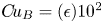 $C\!u_{B} = (\epsilon ) 10^{2}$. Thus, in figure 12(d), we compare the two components, keeping
 $\epsilon$ as an independent variable. Since the current analysis is valid for asymptotically thin interaction layers, we vary
 $\epsilon$ from
 $10^{-4}$ to
 $10^{-2}$. Physically,
 $C\!u_{\lambda }/C\!u_{B} = \epsilon ^{-1}$ corresponds to the disparity in shear rates in the inner and outer regions. For
 $\epsilon \sim 10^{-4}$, the shear rate inside the interaction layer is very high and thus the contribution from
 $U_{\lambda _{1}}$ dominates that from
 $U_{B}$. As
 $\epsilon$ increases (i.e. thickness of interaction layer), the shear in the interaction layer decreases, which increases the magnitude of
 $U_{B}/U_{\lambda _{1}}$. This continues until
 $U_{B}$ reaches a plateau. (The above results are for
 $\zeta =16$. The Appendix shows the effect
 $\zeta$ on the swimming velocity.)
The contribution from both non-Newtonian components is modest in magnitude. In context of electrophoresis, Khair et al. (Reference Khair, Posluszny and Walker2012) also reported a similar enhancement and trends in a shear-thinning medium. Analogous to their study, our result (3.10) also reveals that the shear-thinning modification of the slip does not add a size dependency to the motion induced due to self-diffusiophoresis. On the other hand, the modification due to bulk non-Newtonian stresses adds a size dependency (it enters through the bulk Carreau number).
4. Conclusions
The results of the current study reveal the effects of fluid rheology on the diffusio-osmotic slip over an active surface and its consequence on the mobility of a Janus particle. Using matched asymptotic expansions in conjunction with perturbation theory, we derived the modification to slip velocity for a second-order fluid. Our result (2.19), for an axisymmetrically active Janus particle, shows that the polymeric stress significantly alters the slip velocity, and is valid for low to moderate advective effects. The proportionality to second tangential gradients results in a sharp reversal of the surface slip, triggered by large gradient in polymeric stress across the discontinuity of surface activity. This explains the generation of extensional flow across a step change in activity observed by Natale et al. (Reference Natale, Datt, Hatzikiriakos and Elfring2017). An examination of characteristic scales reveals that the localized reversal of slip velocity is a result of mathematical inconsistency: a consequence of employing the activity as a step function, which can be overcome by choosing a smooth (sigmoidal) function. The results reveal that the polymer elasticity tends to generate local elongational flows across the transition of surface activity. We also explored the effects of attractive and repulsive interaction between the solute molecules and Janus particle. Using the reciprocal theorem, we found that the modification in the slip has an effect on the swimming velocity which is comparable to that arising from bulk viscoelastic stresses (Datt et al. Reference Datt, Natale, Hatzikiriakos and Elfring2017).
We further applied the framework to a generalized weakly shear-thinning fluid and obtained the modification to slip velocity (3.10). Employing a Carreau-fluid model, we found that the shear-thinning effects marginally increase the slip velocity, provided the time scale associated with the shear in the interaction layer is asymptotically smaller than the fluid relaxation time. Using the reciprocal theorem, we showed an enhancement in the swimming velocity due to modification in slip. For an asymptotically thin interaction layer, this enhancement dominates the retardation caused by the bulk non-Newtonian stress.
Another key implication of our results is that the modification in slip provides an estimate of the hydrodynamic disturbance around an active particle for weak non-Newtonian effects. This can be a significant contribution towards accurate modelling of the interaction of two or more active particles in polymeric fluids (Stark Reference Stark2018; Rallabandi, Yang & Stone Reference Rallabandi, Yang and Stone2019). Recently, Michelin et al. (Reference Michelin, Montenegro-Johnson, De Canio, Lobato-Dauzier and Lauga2015) and Michelin & Lauga (Reference Michelin and Lauga2019) have designed ‘phoretic pumps’ which can transport fluids without the need of applying pressure difference across the channel. This can be helpful in transportation of biological fluids through narrow channels. The flow in such systems occurs due to local concentration gradients, arising either from geometric variation (Michelin et al. Reference Michelin, Montenegro-Johnson, De Canio, Lobato-Dauzier and Lauga2015; Lisicki et al. Reference Lisicki, Michelin and Lauga2016) or variation in surface activity (Michelin & Lauga Reference Michelin and Lauga2019). Since our results are applicable to a general diffusio-osmotic slip, they should be useful in modelling the flow of complex fluids through such pumps.
The current work and previous investigations corresponding to the active motion in complex fluids (Datt et al. Reference Datt, Natale, Hatzikiriakos and Elfring2017; Natale et al. Reference Natale, Datt, Hatzikiriakos and Elfring2017) have assumed the diffusivity of solute molecules to be constant. This might be reasonable in the limit of weak non-Newtonian effects, but may lead to imprecise conclusions for fluid mediums exhibiting strong non-Newtonian behaviour, as the Stokes-Einstein equation fails in describing diffusion in complex media. Recently, Makuch et al. (Reference Makuch, Hołyst, Kalwarczyk, Garstecki and Brady2020) devised a relationship between translational and rotational diffusion coefficients which depends on the size of solute. Such theoretical formulation can provide a database for a precise description of diffusion in various complex fluids. Such data can be employed in a theoretical framework similar to that devised by Vrentas & Vrentas (Reference Vrentas and Vrentas2003) and Tiefenbruck & Leal (Reference Tiefenbruck and Leal1980) who studied the effect of diffusion in non-Newtonian flows. Further research in this direction can help in a better understanding of self-propulsion through the mediums which exhibit significant deviations from the Newtonian behaviour.
Acknowledgments
The financial support from Indian Ministry of Human Resource Development is gratefully acknowledged. The authors would like to thank anonymous referees of this work for their valuable comments and suggesting to us to directly compare the two non-Newtonian components of swimming velocity. A.C. thanks Sébastien Michelin for pointing out the importance of transition length for sigmoidal activity. The authors also thank Marco De Corato and Dipin Pillai for their useful suggestions.
Declaration of interests
The authors report no conflict of interest.
Supplementary material
Supplementary material is available at https://doi.org/10.1017/jfm.2020.428.
Appendix. Additional results for the shear-thinning fluid
Figure 13(a) shows the velocity field inside the thin interaction layer for Carreau fluid and a sigmoidal activity transition (2.28). The contours bear a close resemblance to those for Newtonian fluids figure 8(a). Thus, we plot the difference between the two in figure 13(b). The local viscosity reduction due to shear-thinning increases the velocity inside the inner region and consequently the slip (as observed in figure 12a). This enhancement is symmetric about  $\theta _{c}$.
Tangential velocity contours inside the interaction layer for (a) Newtonian fluid and (b) shear-thinning Carreau fluid. The arrows depict the velocity field vector  $\hat {\boldsymbol {u}}_{1}^{(0)}$. Other parameters:
 $\chi =0.1$,
 $n=0.25$,
 $\zeta =16$,
 $\hat {\psi }(\xi ) = -{\rm e}^{-\xi }$.

Figure 14 shows the results for repulsive exponential interactions between the solute molecules and active surfaces. Figure 14(a) depicts the slip velocity, which is qualitatively reversed in comparison to that depicted for the attractive interactions (see figure 12a). The magnitude is lower in this case because the adsorption coefficient is reduced in repulsive interactions (Anderson et al. Reference Anderson, Lowell and Prieve1982). Figure 14(b) shows that the enhancement caused by  $U_{\lambda _{I}}$ is qualitatively similar to that observed in the case of attractive interactions. As the ratio
 $U_{B}/U_{\lambda _{0}}$ is independent of mobility coefficient, its profile is identical to figure 12(c).
(a) The dashed line represents the Newtonian slip velocity. The solid line represents the variation of total slip velocity along the polar angle for  $\hat {\psi }(\xi )=+ {\rm e}^{-\xi }$ and
 $C\!u_{\lambda }=100$. (b) Variation of swimming velocity (arising from the surface slip) with
 $C\!u_{\lambda }$, for three different surface coverage (
 $\theta _{c}$). Other parameters:
 $\chi =0.1$,
 $n=0.25$,
 $\zeta =16$.

As in § 2.4, we now analyse the effect of transition parameter ( $\zeta$) on the non-Newtonian components of the swimming velocity. Here,
 $\zeta$ determines the magnitude of shear inside the interaction layer and slip velocity. Figure 15(a) shows that the transition parameter has a small effect on the contribution due to slip modification. This is because,
 $M_{1}$ has a weak dependency on
 $\zeta$ (see figure 11), which provides
 $U_{\lambda _{1}}$ a
 $\zeta$ dependency similar to that of
 $U_{\lambda _{0}}$ (cf. (3.14) and (2.31a,b)). Thus, the ratio (
 $U_{\lambda _{1}}/U_{\lambda _{0}}$) does not change substantially with
 $\zeta$. Figure 15(b) shows that, at low to moderate
 $C\!u_{B}$, the contribution due to bulk stresses decreases significantly with decrease in
 $\zeta$ (as the shear rate
 $|\gamma _{0}|$ reduces). As
 $C\!u_{B}$ increases, the bulk non-Newtonian stresses reduce because the flow approaches a Newtonian state, i.e.
 $\mu ^{*} \rightarrow \mu ^{*}_{\infty }$. For a lower
 $\zeta$, the shear (
 $|\gamma _{0}|$) is reduced and thus, the reduction in non-Newtonian stresses occurs at a higher
 $C\!u_{B}$. As a result, the trend reverses for
 $C\!u_{B} > 10$ in figure 15(b); the ratio for
 $\zeta =4$ is greater than that corresponding to
 $\zeta =8,16$. Figure 15(c) compares the two components over the range of interaction layer thickness.
Analysis of different components of swimming velocity for three different transition parameters:  $\zeta =4$ (, pink),
 $\zeta =8$ (, black), and
 $\zeta =16$ (, blue). (a) Contribution from the slip modification to the swimming velocity for different surface coverages and
 $\hat {\psi }(\xi ) = -{\rm e}^{-\xi }$. (b) Bulk stress contribution to the swimming velocity for different surface coverages. (c) Comparison of two non-Newtonian contributions to the swimming for
 $Cu_{\lambda }=10^{2}$. Other parameters:
 $\chi =0.1$,
 $n=0.25$,
 $\theta _{c}={\rm \pi} /2$.